On photons and matter inversion spheres
from complex super-spinars accretion structures

Abstract

Our analysis focus on the dragging effects on the accretion flows and jet emission in Kerr super-spinars. These attractors are characterized by peculiar accretion structures as double tori, or special dragged tori in the ergoregion, produced by the balance of the hydrodynamic and centrifugal forces and also effects of super-spinars repulsive gravity. We investigate the accretion flows, constituted by particles and photons, from toroids orbiting a central Kerr super-spinar. As results of our analysis, in both accretion and jet flows, properties characterizing these geometries, that constitute possible strong observational signatures or these attractors, are highlighted. We found that the flow is characterized by closed surfaces, defining inversion coronas (spherical shell), with null the particles flow toroidal velocity ($u^{\phi}=0$) embedding the central singularity. We proved that this region distinguishes proto-jets and accretion driven flows, co-rotating and counter-rotating flows. Therefore in both cases the flow carries information about the accretion structures around the central attractor, demonstrating that inversion points can constitute an observational aspect capable of distinguishing the super-spinars.

I Introduction

The study of possible astrophysical signatures for Kerr super-spinars constitutes an extensive and debated literature on a huge variety of astrophysical phenomena–see for example [1, 2, 3, 4, 5, 6, 7, 8, 9, 10, 11, 12, 13, 14].

In the present analysis, we discuss newly introduced observationally relevant astrophysical phenomena which can expose distinctions between Kerr Naked Singularities (NSs) and Black holes (BHs). We implement this analysis in the accretion and jet emission frame investigating the accretion tori flow and jet emission in the super-spinnar gravitational field.

Inversion points investigated here are points of vanishing toroidal velocity of the particles and photons as related to distant static observers, therefore defined by the condition $u^{\phi}=0$ (or equivalently $\Omega=0$) on the flow particles and photons velocities (relativistic angular velocity). This condition defines a spherical surface, the inversion sphere, embedding the central attractor, where $\Omega=0$. The inversion sphere is independent from the normalization condition on the flow components at the inversion point, therefore describes equivalently photons and timelike particles. Jet emission and accretion flow from the orbiting structures define a closed region surrounding the central attractors bounded by an inner and outer inversion sphere, and fixed only by the spin–mass ratio of the attractor. This closed region (spherical shell), defined inversion coronas, filled with null particles flow toroidal velocity ($u^{\phi}=0$) distinguishes proto-jets and accretion driven flows, co-rotating and counter-rotating flows. The location and topology of this sphere carries information about details of the accretion structures around the central attractor. Therefore an inversion corona is as a valid astrophysical tracer distinguishing Kerr super-spinar solutions from Kerr BH solutions, providing also possible strong observational signature of the NSs.

This analysis follows paper [15], where the case of Kerr BH attractors has been considered, while in [44] a comparison between BH and NS inversion sphere is discussed.

The inversion points in the super-spinner geometries are related to a combination of the repulsive gravity effects and the frame dragging effects, typical of the NSs ergoregion. Toroidal configurations around the central super-spinning attractor have been thoroughly characterized in a several studies, here we discuss the accretion flow velocity components, energy and momentum at the inversion points taking into account the peculiar NS causal structure and the frame dragging effects from the NSs ergoregions.

We detail, the fluid inversion points driven by the orbiting toroidal structures. To fix the discussion we considered geometrically thick general relativistic hydrodynamic (GRHD) disks, centered on the equatorial plane of the central attractor, which is also the tori symmetry plane. It should be noted that the inversion points analysis is however independent from an eventual tilted angle, and the assumption of coplanar tori is in fact not necessary. More precisely we consider barotropic, radiation pressure supported accretion tori, cooled by advection, with low viscosity and opaque, with super-Eddington luminosity (high matter accretion rates) [16, 17, 18, 19]. This model (Polish doughnut) is widely used in literature as the initial conditions of the GRMHD (magnetohydrodynamic) evolution of accretion disks [20, 21, 22, 23, 24]. In the GRHD barotropic models, the time scale of the dynamical processes $\tau_{dyn}$ (driven by gravitational and inertial forces) is much lower than the time scale of the thermal ones $\tau_{therm}$ (including heating and cooling processes, radiation) which is lower than the time scale of the viscous processes $\tau_{\nu}$. In other words, the strong gravitational field of the background is dominant with respect to the dissipative forces, in determining the tori unstable phases [25, 19, 26, 17, 27, 21, 22, 28, 29, 30, 31, 32]. Within this approximation, during the dynamical processes, the functional form of the angular momentum and entropy distribution in the fluid, depends on the system initial conditions and not on the the details of the dissipative processes.

The accretion process turns therefore to be regulated by the mass loss in the outer toroid Roche lobe overflow, associated to the occurrence of the surface cusp. The instability process follows the un-balance of the gravitational, inertial forces, and the pressure gradients in the fluid. This is a important self-regulated process, which turns out to locally stabilize the accreting torus from the thermal and viscous instabilities and it globally stabilizes the torus from the Papaloizou&Pringle instability[33, 34, 35, 19, 17, 18].).

As for the BH case, analyzed in [15], the flow inversion points in the NS spacetimes, define the inversion sphere as a closed and regular surface determined by the constant fluid specific angular momentum $\ell$. Whereas the turning corona is defined by the range of location of the disk inner edge or the proto-jets cusps for accretion driven or proto-jets driven flows.

Therefore, although the inversion points do not depend on the details of the accretion processes, or the precise location of the tori inner edge, in our analysis the flow of photons and free-falling particles are driven from the inner edge (the toroidal surface cusp) of the accretion disk or proto-jets (open, cusped configuration).

In general, the concept of accretion disks inner edge depends on the details of the accretion process. However analytic models of accretion tori fix a certain radius $r_{\times}$, inner edge, which is usually an unstable geodesic circular orbit, the cusp, as a theoretical radius distinguishing the accretion flows in (free falling) particles from the region $r<r_{\times}$, and at $r>r_{\times}$, defines the accretion torus up to an outer edge $r_{outer}$ [36, 37, 38] [39, 40, 41, 42, 43]. For a stellar attractor, the inner edge is generally located near the star surface, for BHs and the NSs the inner edge lies between the marginally bound circular orbit and the marginally stable circular orbit. The proto-jets have a cusp in the orbital range defined by the marginally circular orbit (usually a photon orbit) and marginally bound circular orbit. Therefore, the fluid specific angular momentum at these orbits defines the accretion driven and defines the proto-jets driven inversion coronas respectively. The morphological structure of the jets and particularly the velocity components on the central axis of rotation constitute an important topic of jet emission collimation, thus for the proto-jets analysis we consider in particular the presence of flow inversion point in the direction of the rotational axis of the central attractors (vertical direction).

More in details, this article plan is as follows:

In Sec. (II) we introduce the spacetime metric. The toroidal structures are discussed in Sec. (II.1).

The inversion points are analyzed in Sec. (III). In Sec. (III.1) we define the flow inversion points and in Sec. (III.2) flow inversion points are related to the orbiting structures defining accretion driven and proto-jets driven inversion coronas.

In Sec. (III.2.1) we address the special case of double tori with equal specific angular momentum. Tori and inversion points for $\ell=\pm a$ are studied in Sec. (III.2.2). Excretion driven inversion points and torus outer edges are focused in Sec. (III.2.3). The location of inversion points in relation to the ergoregion is discussed in Sec. (III.2.4). NSs are distinguished from the BHs by the presence of double inversion points on planes different from the equatorial, we discuss this aspect in Sec. (III.2.5). Proto-jets driven inversion points and inversion points verticality are focused in Sec. (III.2.6): Some notes on the inversion coronas thickness and slow counter-rotating inversion spheres are in Sec. (III.2.7). We conclude in Sec. (III.2.8) with further notes on the flow inversion points from orbiting tori. Sec. (IV) contains discussion and final remarks. Three appendix sections follow: some more in depth notes on the tori models are in Sec. (A), relative location of the inversion points in accreting flows is the focus of Sec. (B). Further notes on the co-rotating flows inversion points are in Sec. (C).

II The Kerr spacetime metric

The Kerr spacetime metric reads

$$ds^{2}=-\left(1-\frac{2Mr}{\Sigma}\right)dt^{2}+\frac{\Sigma}{\Delta}dr^{2}+\Sigma d\theta^{2}+\left[(r^{2}+a^{2})+\frac{2Mra^{2}}{\Sigma}\sigma\right]\sigma d\phi^{2}-\frac{4rMa}{\Sigma}\sigma dtd\phi,$$ (1)

In the Boyer-Lindquist (BL) coordinates $\{t,r,\theta,\phi\}$, where

$$\Delta\equiv a^{2}+r^{2}-2rM\quad\mbox{and}\quad\Sigma\equiv a^{2}(1-\sigma)+r^{2},\quad\sigma\equiv\sin^{2}\theta.$$ (2)

Parameter $a=J/M\geq 0$ is the metric spin, where total angular momentum is $J$ and the gravitational mass parameter is $M$. The Kerr naked singularities (NSs) have $a>M$. A Kerr black hole (BH) is defined by the condition $a\in[0,M]$ with Killing horizons horizons $r_{-}\leq r_{+}$ where $r_{\pm}\equiv M\pm\sqrt{M^{2}-a^{2}}$). The extreme Kerr BH has dimensionless spin $a/M=1$ and the non-rotating case $a=0$ is the Schwarzschild BH solution.

The outer and inner stationary limits $r_{\epsilon}^{\pm}$ (ergosurfaces), are given by

$$r_{\epsilon}^{\pm}\equiv M\pm\sqrt{M^{2}-a^{2}(1-\sigma)}$$ (3)

respectively. We also introduce the function $\sigma_{erg}:r=r_{\epsilon}^{\pm}$:

$$\sigma_{erg}\equiv\frac{(r-2M)r}{a^{2}}+1$$ (4)

The region $[r_{\epsilon}^{-},r_{\epsilon}^{+}]$ is the ergoregion. There is $r_{\epsilon}^{-}=0$ and $r_{\epsilon}^{+}=2M$ in the equatorial plane $\theta=\pi/2$ ($\sigma=1$), and $r_{+}<r_{\epsilon}^{+}$ on $\theta\neq 0$. More precisely there is

$$g_{tt}>0\quad\mbox{for}:a\geq M\quad\left(\sigma=\sigma_{\epsilon}^{+},r=r_{\epsilon}^{-}\right);\left(\sigma\in]\sigma_{\epsilon}^{+},1[,r\in[r_{\epsilon}^{-},r_{\epsilon}^{+}]\right);\left(\sigma=1,r\in]0,2M]\right);$$

$$\mbox{where}\quad\sigma_{\epsilon}^{+}\equiv\frac{a^{2}-M^{2}}{a^{2}}.$$ (5)

NS poles $\sigma=0$ are associated to $g_{tt}<0$ for $a\geq 0$ and $r\geq 0$. In the following, where appropriate, to easy the reading of complex expressions, we will use the units with $M=1$ (where $r\rightarrow r/M$ and $a\rightarrow a/M$).

The equatorial circular geodesics are confined on the equatorial plane as a consequence of the metric tensor symmetry under reflection through the plane $\theta=\pi/2$. We consider the following constant of geodesic motions

$$\mathcal{E}=-(g_{t\phi}\dot{\phi}+g_{tt}\dot{t}),\quad\mathcal{L}=g_{\phi\phi}\dot{\phi}+g_{t\phi}\dot{t},$$ (6)

$$\mbox{where}\quad g_{ab}u^{a}u^{b}=\kappa\mu^{2},\quad u^{t}=\frac{g_{\phi\phi}\mathcal{E}+g_{t\phi}\mathcal{L}}{g_{t\phi}^{2}-g_{\phi\phi}g_{tt}},\quad u^{\phi}=-\frac{g_{t\phi}\mathcal{E}+g_{tt}\mathcal{L}}{g_{t\phi}^{2}-g_{\phi\phi}g_{tt}},$$

with $u^{a}\equiv\{\dot{t},\dot{r},\dot{\theta},\dot{\phi}\}$ where $\dot{q}$ indicates the derivative of any quantity $q$ with respect the proper time (for $\mu>0$) or a properly defined affine parameter for the light–like orbits (for $\mu=0$), and $\kappa=(\pm,0)$ is a normalization constant ($\kappa=-1$ for test particles).

Quantity $\xi_{\phi}=\partial_{\phi}$ is the rotational Killing field and $\xi_{t}=\partial_{t}$ is the Killing field representing the stationarity of the Kerr background. The constant $\mathcal{L}$ in Eq. (6) can be interpreted as the axial component of the angular momentum of a test particle following timelike geodesics and $\mathcal{E}$ represents the total energy of the test particle related to the radial infinity, as measured by a static observer at infinity. The specific angular momentum is

$$\ell\equiv\frac{\mathcal{L}}{\mathcal{E}}=-\frac{g_{\phi\phi}u^{\phi}+g_{\phi t}u^{t}}{g_{tt}u^{t}+g_{\phi t}u^{\phi}}=-\frac{g_{t\phi}+g_{\phi\phi}\Omega}{g_{tt}+g_{t\phi}\Omega},\quad\Omega\equiv\frac{u^{\phi}}{u^{t}}=-\frac{g_{t\phi}+g_{tt}\ell}{g_{\phi\phi}+g_{t\phi}\ell}$$ (7)

where $\Omega$ is the relativistic angular velocity. For a circularly orbiting test particle, particle counter–rotation (co-rotation) is defined by $\mathcal{L}a<0$ ($\mathcal{L}a>0$). The Kerr NS background geodesic structure is constituted by the radii $\{r_{\gamma}^{\pm},r_{mbo}^{\pm},r_{mso}^{\pm}\}$, marginally circular (photon) orbit, marginally bounded orbit, and marginally stable orbit respectively for counter-rotating $(+)$ and co-rotating $(-)$ motion–see Figs (1). The spacetime geodesic structure regulates test particles circular motion and some key aspects of accretion disks physics–see Table (1). In Sec. (II.1) we discuss further the notion of co-rotating and counter-rotating accretion tori in NSs spacetimes.

II.1 Co-rotating and counter-rotating accretion tori in NSs spacetimes

${r}_{[mbo]}^{\pm}:\;\ell^{\pm}(r_{mbo}^{\pm})=\ell^{\pm}({r}_{[mbo]}^{\pm})\equiv{\ell_{mbo}^{\pm}},\quad r_{[\gamma]}^{\pm}:\ell^{\pm}(r_{\gamma}^{\pm})=\ell^{+}(r_{[\gamma]}^{+})\equiv\ell_{\gamma}^{+}$

$r_{\gamma}^{\pm}<r_{mbo}^{\pm}<r_{mso}^{\pm}<{r}_{[mbo]}^{\pm}\quad\mbox{and}\quad{r}_{[mbo]}^{+}<r_{[\gamma]}^{+}<r_{\gamma}^{-}\equiv 0$,

$\ell^{\pm}\in\mathbf{L_{1}^{\pm}}\equiv]\ell^{\pm}_{mbo},\ell^{\pm}_{mso}[$: quiescent and cusped tori. $r_{\times}\in]r_{mbo}^{\pm},r_{mso}^{\pm}]$, $r_{center}\in]r_{mso}^{\pm},r_{[mbo]}^{\pm}]$;

$\ell^{\pm}\in\mathbf{L_{2}^{\pm}}\equiv[\ell^{\pm}_{\gamma},\ell^{\pm}_{\mathrm{mbo}}[$: quiescent tori and proto-jets. $r_{j}\in]r_{\gamma}^{\pm},r_{mbo}^{\pm}]$ $r_{center}\in]r_{[mbo]}^{\pm},r_{[\gamma]}^{\pm}]$;

$\ell^{\pm}\in\mathbf{L_{3}^{\pm}}:\ell^{\pm}<\ell^{\pm}_{\gamma}$: quiescent tori, $r_{center}>r_{[\gamma]}^{\pm}$.

Table 1: Co-rotating and counter-rotating tori in Kerr NSs. $\ell$ is the fluid specific angular momentum. Radii $r_{mso}^{-}=\{\bar{r}_{mso}^{-},\tilde{r}_{mso}^{-}\}$, are the marginally stable orbits related to the motion $\ell^{-}\gtrless 0$, where $r_{mso}^{-}=\bar{r}_{mso}^{-}$ for spin $a>a_{1}$ and $r_{mso}^{-}=\tilde{r}_{mso}^{-}$ for $a\in]M,a_{1}]$ and $\bar{r}_{mso}^{-}=\tilde{r}_{mso}^{-}$ on $a_{1}$–Figs (1). Spin $a_{1}$ is defined in Table (2). For simplicity of notation, when it is not necessary to specify, we will use the abbreviated notation $r_{mso}^{-}$ for $\{\bar{r}_{mso}^{-},\tilde{r}_{mso}^{-}\}$. We adopt the notation $q_{\bullet}\equiv q(r_{\bullet})$ for any quantity $q$ evaluated on a radius $r_{\bullet}$. Radii $\{r_{\gamma}^{\pm},r_{mbo}^{\pm}\}$, are the marginally circular (photon) orbit and the marginally bounded orbit for $\ell^{+}$ and $\ell^{-}$ specific angular momentum. Relation between radii $\{r_{mso}^{\pm},r_{\gamma}^{\pm},r_{mbo}^{\pm}\}$ characterizes fluids with $\ell^{+}$ and $\ell^{-}$ at NSs spins $a>a_{2}$–see Table (2)–where there is $r_{\gamma}^{-}\equiv 0$. Radii $\{r_{[mbo]}^{\pm},r_{[\gamma]}^{\pm}\}$ constitute the Kerr geometry extended geodesic structure. There is $\ell_{\gamma}^{-}=a$ and $r_{[\gamma]}^{-}=a^{2}$–see also Figs (1).

We analyze two families of accretion tori, governed by the distribution of specific angular momentum on the equatorial plane,

$$\ell^{\mp}\equiv\frac{a^{3}\mp r^{3/2}\Delta-a(4-3r)r}{a^{2}-(r-2)^{2}r},$$ (8)

[19, 44, 45, 26]. Toroids are full GRHD (barotropic) Polish doughnut (PD) models, composed by one -particle-species fluids orbiting on the equatorial plane (the tori symmetry plane) of the central attractor, and parameterized with constant specific angular momentum $\ell^{\pm}=$constant.

The fluid dynamics is governed by the Euler equation only, expressible through an effective potential function, $V_{eff}(r;\ell,a)$, encoding the centrifugal and gravitational components of the force balance. The pressure gradients are regulated by the gradients of an effective potential function for the fluid. Toroidal configurations are characterized by a maximum of the pressure and density (torus center $r_{center}$) and, eventually, a vanishing of pressure point, tori cusps $r_{\times}$ and proto-jets cusps $r_{j}$. Proto-jets are open, cusped, HD toroidal configurations, with matter funnels along the attractor rotational axis. The torus edges are solutions of $V_{eff}^{2}=K^{2}=$constant and there is $K=K_{\times}$ for the cusped tori edges. There is $K_{\times}<1$ for tori cusps and $K_{\times}\geq 1$ for proto-jets cusps–see Table (1), these values can be obtain from the function $K(r)\equiv V_{eff}(r;\ell(r),a)$.

Geometrically thick tori considered in this analysis are well known and widely used in literature–see for example [19, 60]. In this section we outline some fundamental aspects for the analysis of the turning points, constituting the constraints used in the second part of this work, while in Sec. (A) we summarize some in-depth aspects of these models.

We shall investigate the "disk–driven" free–falling accretion flow composed by matter and photons, and the case of "proto-jets (or jets) driven" flows.

In this section we discuss further the notion of co-rotation and counter-rotation in NSs spacetimes.

We introduce the radii $r_{0}^{\pm}<r_{\epsilon}^{+}=2M:\mathcal{L}=\ell=0$, and $r_{\delta}^{\pm}:\mathcal{E}=0,\mathcal{L}>0$ where $r_{0}^{-}<r_{\delta}^{-}<r_{\delta}^{+}<r_{0}^{+}$, showed in Figs (1) (explicit forms are in [44]) and spins $a_{j}$ with $j\in\{0,9\}$ and $\{a_{\mathbf{i}},a_{\mathbf{ii}},a_{\mathbf{iii}},a_{\mathbf{iv}}\}$, in Table (2),

$a_{0}\equiv\frac{4}{3}\sqrt{\frac{2}{3}}M=1.08866M:r_{\delta}^{+}=r_{\delta}^{-}$,	$a_{1}\equiv 1.28112M$,	$a_{2}\equiv\frac{3\sqrt{3}}{4}=1.29904M:r_{0}^{+}=r_{0}^{-}$
$a_{3}\equiv\sqrt{3}M$	$a_{4}\equiv 3.7195M:r_{\gamma}^{+}=r^{-}_{[mbo]}$,	$a_{5}\equiv 8M:r^{-}_{[mbo]}=r_{mbo}^{+}$
$a_{6}\equiv 9M:r_{\gamma}^{+}=\bar{r}_{mso}^{-}$	$a_{7}\equiv 22.3137M:r_{\gamma}^{+}=r_{mbo}^{-}$	$a_{8}\equiv 24.6082M:r^{-}_{[mbo]}=r_{mso}^{+}$
$a_{9}\equiv 45.6274M:r_{mbo}^{+}=\bar{r}_{mso}^{-}$	$a_{\mathbf{i}}\equiv 4.12311M:r_{mso}^{+}={r}_{[\gamma]}^{-}$	$a_{\mathbf{ii}}\equiv 3M:r_{mbo}^{+}={r}_{[\gamma]}^{-}$
$a_{\mathbf{iii}}\equiv 2.23607M:r_{\gamma}^{+}={r}_{[\gamma]}^{-}$	$a_{\mathbf{iv}}\equiv 1.03886M:r_{mso}^{+}=\tilde{r}_{[mso]}^{-}$,

Table 2: Notable spins in the Kerr NS spacetime. Radii $r$, defining the spin sets are in Table (1). Radii $r_{0}^{\pm}$ and $r_{\delta}^{\pm}$ are defined in Sec. (II.1)– see also Figs (1).

defined by the geodesic properties of the spacetime, showed in Figs (1). Fluid specific angular momentum $\ell=\ell^{+}<0$ defines counter-rotating fluids while $\ell=\ell^{-}\lesseqgtr 0$ distinguishes co-rotating and counter-rotating tori respectively and we summarize the situation in Table (3).

Counter-rotating tori $(\ell<0)$	Co-rotating tori ($\ell>0$)
$\ell=\ell^{+}<0$, $\ell=\ell^{-}<0$ in the ergoregion for $a\in[M,a_{2}]$	$\ell=\ell^{-}>0$ $(\mathcal{L}>0,\mathcal{E}>0)$, for $(r>0,a>a_{2})$
(I) $\ell=\ell^{+}<0$ $(\mathcal{L}<0,\mathcal{E}>0)$ (out of the ergoregion)	$(r\in]0,r_{0}^{-}[\cup]r_{0}^{+},+\infty[,a\in]a_{0},a_{2}[)$ $(\mathcal{L}>0,\mathcal{E}>0)$
(II) $\ell=\ell^{-}<0$, $(\mathcal{L}<0,\mathcal{E}>0)$, in $]r_{0}^{-},r_{\delta}^{-}[\cup]r_{\delta}^{+},r_{0}^{+}[$, for $a\in[M,a_{0}]$.	$(]r_{\delta}^{-},r_{\delta}^{+}[,a\in]M,a_{0}[$ $(\mathcal{L}<0,\mathcal{E}<0)$
and in $]r_{0}^{-},r_{0}^{+}[$, for $a\in]a_{0},a_{2}]$	$r\in]0,r_{0}^{-}[\cup r>r_{0}^{+},a\in]M,a_{0}[$ $(\mathcal{L}>0,\mathcal{E}>0)$

Table 3: Co-rotating and counter-rotating tori in Kerr NSs, $\ell$ is the fluid specific angular momentum. Radii $r_{0}^{\pm}$ and $r_{\delta}^{\pm}$ are defined in Sec. (II.1)– see also Figs (1), spins are defined in Table (1). $\mathcal{E}$ and $\mathcal{L}$ are the test particles energy and angular momentum.

However, $\ell^{-}<0$ with $(\mathcal{L}<0,\mathcal{E}>0)$ in the NS ergoregion, and with co-rotating solutions $\ell^{-}>0$ with $(\mathcal{L}<0,\mathcal{E}<0)$ with negative energy $\mathcal{E}$ are all co-rotating with respect to the static observers at infinity as they correspond to the relativistic angular velocity with respect to static observers at infinity, $\Omega>0$.

The Kerr geodesic structure regulates the accretion disk physics bounding the accreiting disk inner edge (tori cusps) and proto-jets cusps. The cusps are point of the minimum pressure and density in the barotropic toroids–see Sec. (A). The extended geodesic structure includes radii $\{r_{[\gamma]}^{\pm},r_{[mbo]}^{\pm},r_{[mso]}^{\pm}\}$ defined Table (1) and governing the location of the toroidal configurations centers (point of maximum density and pressure in the barotropic tori) [51, 52, 53, 54].

Table (1) shows the situation for fluids with $\ell^{+}$, and for fluids with $\ell=\ell^{-}$ orbiting in NS spacetimes with spins $a>a_{2}$.

NSs with spin $a\in]M,a_{2}]$ and fluids with $\ell^{-}$ are characterized by a more articulated structure and we summarized this situation in Figs (1). For tori centers and cusps located on $r_{0}^{\pm}$ there is $\ell=\mathcal{L}=0$ (tori in these limiting cases are considered in [44]). On $r_{\delta}^{\pm}$ ("center" and "cusp" respectively) there is $\mathcal{E}=0$ ($\ell$ is not well defined). For $a\in[M,a_{2}]$, there can be tori with $\ell^{-}<0$ and ($\mathcal{E}>0,\mathcal{L}<0$) in the ergoregion and tori with $\ell^{-}>0$ and ($\mathcal{E}<0,\mathcal{L}<0$). There can be double tori system with $\ell=\ell^{+}=\ell^{-}<0$ or $\ell=\ell^{-}>0$, and this case is detailed in Sec. (III.2.1).

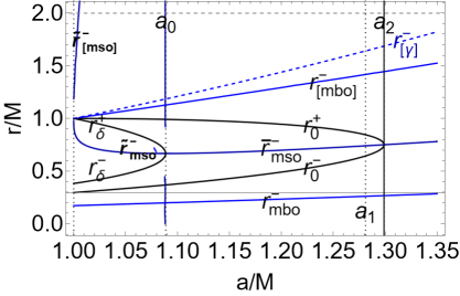
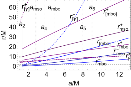
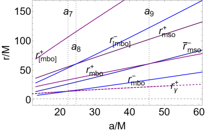
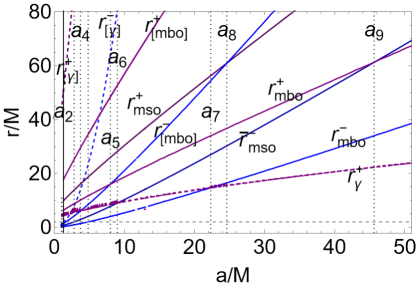
Figure 1: Analysis of the extended geodetic structure of the Kerr NS, constraining tori with fluid angular momentum $\ell=\ell^{\pm}$. Spins $\{a_{0},a_{1},a_{2},a_{4},a_{5},a_{6},a_{7},a_{8},a_{9}\}$ are defined in Table (2). Radius $r_{\gamma}^{+}$ is the counter–rotating last circular orbit relative to counter-rotating fluids with $\ell=\ell^{+}<0$, radius $r_{\epsilon}^{+}=2M$, is the outer ergosurface on the equatorial plane. $\{r_{mso}^{\pm},r_{mbo}^{\pm}\}$ are the marginally stable orbit and marginally bounded orbits relative to fluids with $\ell^{\pm}$ respectively. Radii $\{r_{[mso]}^{\pm},r_{[mbo]}^{\pm},r_{[\gamma]}^{+}\}$ are defined on Table (1). On radii $r_{0}^{\pm}$ momenta are $\mathcal{L}(r_{0}^{\pm})=0$, and there is $\mathcal{E}(r_{\delta}^{\pm})=0$.

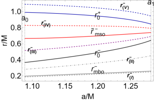
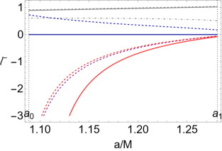
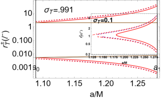
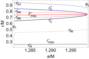
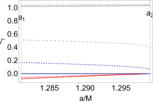
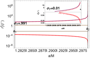
Figure 2: Analysis of the flow inversion point radius $r_{\mbox{\scriptsize{{T}}}}^{\pm}$ with fluid specific angular momentum $\ell=\ell^{-}$. (For $\ell^{-}>0$ inversion points are only for spacelike particles with $(\mathcal{E}<0,\mathcal{L}<0)$.) Spins $\{a_{0},a_{1},a_{2}\}$ are defined in Table (2). Radii $r_{mso}^{-}=\{\bar{r}_{mso}^{-},\tilde{r}_{mso}^{-}\}$ are the marginally stable orbit, radius $r_{mbo}$ is the marginally bounded orbit. There is $\sigma\equiv\sin^{2}\theta$ ($\sigma=1$ is the equatorial plane). There is $r_{0}^{\pm}:\mathcal{L}=0$, where $\mathcal{L}$ is the test particle angular momentum and $r_{\delta}^{\pm}:\mathcal{E}=0$ where $\mathcal{E}$ is the test particle energy. Radii $r/M$ (left panels) and fluid specific angular momentum $\ell^{-}$ (center panels) are plotted as functions of $a/M$, inversion point radius $r_{\mbox{\scriptsize{{T}}}}^{\pm}$ is shown for different planes signed on the panels (right panels). See also Figs (3). There is $r_{\{I\}}^{-}\equiv r_{mbo}^{-}-0.01,r_{\{II\}}^{-}\equiv\left(r_{0}^{-}-r_{mbo}^{-}\right)/2+r_{mbo}^{-},r_{\{III\}}^{-}\equiv r_{mso}^{-}-\left(r_{mso}^{-}-r_{0}^{-}\right)/2,r_{\{IV\}}^{-}\equiv r_{0}^{+}-\left(r_{0}^{+}-r_{mso}^{-}\right)/2,r_{\{V\}}^{-}\equiv r_{0}^{+}+0.1$.

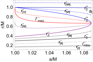
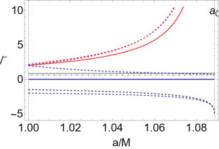
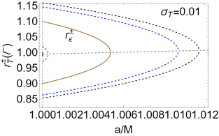
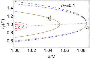
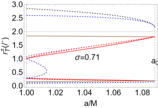
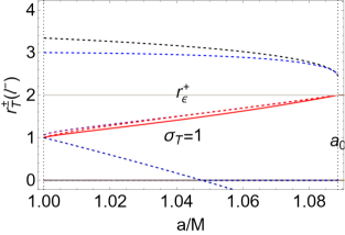
Figure 3: Analysis of the flow inversion point radius $r_{\mbox{\scriptsize{{T}}}}^{\pm}$ for different planes $\sigma\equiv\sin^{2}\theta$ signed on the panels, in the spin range is $a\in[M,a_{0}]$, with fluid specific angular momentum $\ell=\ell^{-}$. Radii $r_{mso}^{-}=\{\bar{r}_{mso}^{-},\tilde{r}_{mso}^{-}\}$ are the marginally stable orbit, radius $r_{mbo}$ is the marginally bounded orbit. There is $r_{0}^{\pm}:\mathcal{L}=0$, where $\mathcal{L}$ is the test particle angular momentum and $r_{\delta}^{\pm}:\mathcal{E}=0$ where $\mathcal{E}$ is the test particle energy. Left panels show radii $r/M$ as functions of the NS spin $a/M$. Center panels show the fluid specific angular momentum $\ell^{-}$, evaluated on the left panel radii, as function of $a/M$. Right panels: inversion radius $r_{\mbox{\scriptsize{{T}}}}^{+}>0$ on different planes, evaluated on the momenta and radii of the center and left panels. Spins $\{a_{0},a_{1},a_{2}\}$ are defined in Table (2). There is $r_{[I]}^{-}\equiv r_{mbo}^{-}-0.01,r_{[\text{II}]}^{-}\equiv\left[r_{0}^{-}-r_{mbo}^{-}\right]/2+r_{mbo}^{-},r_{[\text{III}]}^{-}\equiv\left[r_{\delta}^{-}-r_{0}^{-}\right]/2+r_{0}^{-},r_{[\text{IV}]}^{-}\equiv r_{mso}^{-}-\left[r_{mso}^{-}-r_{\delta}^{-}\right]/2,r_{[V]}^{-}\equiv r_{\delta}^{+}-\left[r_{\delta}^{+}-r_{mso}^{-}\right]/2,r_{[\text{VI}]}^{-}\equiv r_{0}^{+}-\left[r_{0}^{+}-r_{\delta}^{+}\right]/2,r_{[\text{VI}]}^{-}\equiv r_{0}^{+}+0.1$. Brown curves are the outer and inner ergosurfaces $r_{\epsilon}^{\pm}$ respectively. See also Figs (3). (For $\ell^{-}>0$ inversion points are only for spacelike particles with $(\mathcal{E}<0,\mathcal{L}<0)$.)

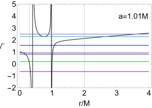
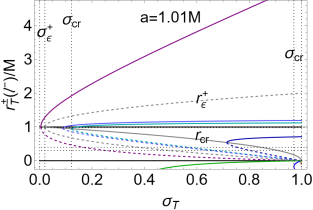
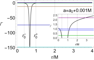
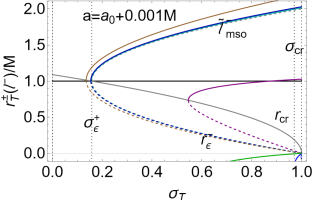
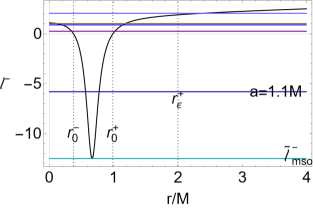
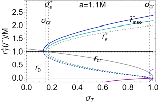
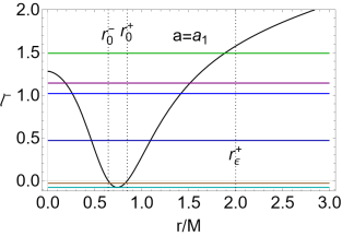
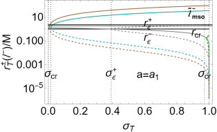
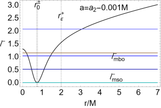
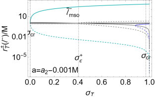
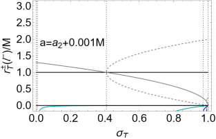
Figure 4: Fluid specific angular momentum $\ell^{-}$ for different spacetime spin $a/M$ signed on the panels, darker-cyan curve is $\ell_{mso}^{-}$, light-blue curve is $\ell_{mbo}$. Marginally circular orbit radius is $r_{mbo}^{-}$ and marginally stable orbits $r_{mso}^{-}=\{\tilde{r}_{mso}^{-},\bar{r}_{mso}^{-}\}$. Horizontal lines select $\ell$ values used for the evaluation of the inversion radii. Inversion points $r_{\mbox{\scriptsize{{T}}}}^{\pm}$ of Eq. (9) of the co-rotating and counter-rotating accretion with $\ell=\ell^{-}$ are shown as functions of the planes $\sigma\equiv\sin^{2}\theta$, where $\sigma=1$ is the equatorial plane, for different NS spin-mass ratio $a/M$ signed on the panels. Plain curves are $r_{\mbox{\scriptsize{{T}}}}^{+}$ while $r_{\mbox{\scriptsize{{T}}}}^{-}$ are dashed curves. For $\ell^{-}>0$ inversion points are only for space-like particles with $(\mathcal{E}<0,\mathcal{L}<0)$. Spins $\{a_{0},a_{1},a_{2}\}$ are defined in Table (2). Radius $r_{\epsilon}^{\pm}$ are the outer and inner ergosurfaces. Plane curve $\sigma_{\epsilon}^{+}$ is defined in Eqs. (5) and radius $r_{cr}$ is in Eq. (10). Limiting plane $\sigma_{cr}$ is function $\sigma_{\sigma a}$ of Eqs (29) on the selected fluid specific angular momentum. There are no inversion points for co-rotating fluids in the geometries with $a>a_{2}$.

III Flow inversion points from orbiting tori with $\ell=\ell^{\pm}$

In this section we analyze the accretion dirven and proto-jets driven flow inversion points. In Sec. (III.1) the flow inversion points are defined, while in Sec. (III.2) we discuss the flow inversion points from the orbiting accretion tori and proto-jets configurations.

III.1 Flow inversion points

The flow inversion points are points of vanishing axial velocity of the flow motion as related to distant static observers, therefore defined by the condition $u^{\phi}=0$ (or equivalently $\Omega=0$) on the flow particles and photons velocities (relativistic angular velocity).

From the definition of $\ell$ and $\mathcal{E}$, Eqs (6) and Eq. (7), and the inversion point definition we obtain:

$$\ell=-\left.\frac{g_{t\phi}}{g_{tt}}\right|_{\mbox{\scriptsize{{T}}}}=-\frac{2ar_{{\mbox{\scriptsize{{T}}}}}\sigma_{{\mbox{\scriptsize{{T}}}}}}{\Sigma_{\mbox{\scriptsize{{T}}}}-2r_{\mbox{\scriptsize{{T}}}}},\quad\mbox{where}$$ (9)

$$r_{\mbox{\scriptsize{{T}}}}^{\mp}=\mp\sqrt{a^{2}\left(\sigma_{\mbox{\scriptsize{{T}}}}+\frac{\sigma_{\mbox{\scriptsize{{T}}}}^{2}}{\ell^{2}}-1\right)-\frac{2a\sigma_{\mbox{\scriptsize{{T}}}}}{\ell}+1}-\frac{a\sigma_{\mbox{\scriptsize{{T}}}}}{\ell}+1,$$

and

$$\sigma_{\mbox{\scriptsize{{T}}}}\equiv\frac{\ell\Delta_{\mbox{\scriptsize{{T}}}}}{a(a\ell-2r_{\mbox{\scriptsize{{T}}}})},\quad r_{\mbox{\scriptsize{{T}}}}^{-}=r_{\mbox{\scriptsize{{T}}}}^{+}=r_{cr}\equiv a\sqrt{1-\sigma_{\mbox{\scriptsize{{T}}}}},$$ (10)

$$\mathcal{E}_{\mbox{\scriptsize{{T}}}}\equiv-g_{tt}({\mbox{\scriptsize{{T}}}})\dot{t}_{\mbox{\scriptsize{{T}}}},\quad\mathcal{L}_{\mbox{\scriptsize{{T}}}}\equiv g_{t\phi}({\mbox{\scriptsize{{T}}}})\dot{t}_{\mbox{\scriptsize{{T}}}},$$

where notation $q_{\mbox{\scriptsize{{T}}}}$ or $q({\mbox{\scriptsize{{T}}}})$ is for any quantity $q$ considered at the inversion point, and $q_{0}=q(0)$ for any quantity $q$ evaluated at the initial point of the (free-falling) flow trajectories.

Therefore, $\mathcal{E}_{\mbox{\scriptsize{{T}}}}$ and $\mathcal{L}_{\mbox{\scriptsize{{T}}}}$ are the energy and momentum of the flow particles at the inversion point. We stress that quantities in Eq (9) and Eq. (10) are independent from the normalization condition, being a consequence of the definition of constant $\{\ell,\mathcal{E},\mathcal{L}\}$. Radius $r_{\mbox{\scriptsize{{T}}}}$ identifies a surface, inversion sphere, which is a general property of the (photon and timelike) orbits in the Kerr NS spacetime, surrounding the central singularity, depending only on $\ell$ where $\Omega=0$. Furthermore, radius $r_{cr}$, of Eq. (10) is a background property, independent explicitly from $\ell$. It si worth noting that there are no timelike and photon-like inversion points with $\ell>0$.

Contrary to the BH case, in the NS there can be two inversion points radii $r_{\mbox{\scriptsize{{T}}}}^{\pm}$. The inversion radii on the poles are well defined in the BH case only ($\lim_{\sigma_{\mbox{\scriptsize{{T}}}}\rightarrow 0}r_{{\mbox{\scriptsize{{T}}}}}^{\pm}=r_{\pm}$). Note that a very large $\ell$ in magnitude is typical of proto-jets emission or quiescent toroids orbiting far from the central attractor for counter-rotating tori (with $\ell=\ell^{+}<0$) or some co-rotating tori with $\ell=\ell^{-}>0$) in a class of slow rotating NSs, in this case the inversion point approaches the ergosurface i.e. $\lim_{\ell\rightarrow\pm\infty}\sigma_{\mbox{\scriptsize{{T}}}}=\sigma_{erg}$ and $\lim_{\ell\rightarrow(\pm\infty)}r_{{\mbox{\scriptsize{{T}}}}}^{\pm}=r^{\pm}_{\epsilon}$, we address this issue with more details in Secs (III.2.4).

Increasing the spin $a/M>0$, the inversion point approaches the equatorial plane $(\sigma_{\mbox{\scriptsize{{T}}}}\leq 1)$. However, for a very faster spinning NS ($a\rightarrow+\infty$) the limit of $r_{\mbox{\scriptsize{{T}}}}=r_{\mbox{\scriptsize{{T}}}}^{\pm}$ for is not well defined.

III.2 Accretion flows turning points

In Sec. (III.1) we discussed the existence of the inversion points considering the condition of constant $\ell=\ell^{\pm}$, independently by the causal conditions on matter at the turning point.

In this section we explore the inversion spheres properties for flows from the accretion disks orbiting NSs, depending on the central attractor spin-mass ratios $a/M$ and fluid specific angular momenta $\ell^{\pm}$.

We focus on the necessary conditions for the existence of the inversion points of the counter-rotating and co-rotating flows, considering first the condition $\ell=$constant and then $\{\ell,\mathcal{E},\mathcal{L}\}$ constant, where a more general necessary condition for the occurrence of the inversion point is $\mathcal{L}<0$. We assume constance of $(\mathcal{E}_{\mbox{\scriptsize{{T}}}},\mathcal{L}_{\mbox{\scriptsize{{T}}}})$ (implied by $\ell=$constant) evaluated at the inversion point with $\dot{t}$>0. We then consider the normalization condition at the inversion point, $g_{\alpha\beta}u^{\alpha}u^{\beta}=\kappa$ (with $u^{\phi}=0$) distinguishing particles and photons in the flow. The matter flow is then related to the orbiting structures, considering toroids with $\ell=\ell^{+}<0$ $(\mathcal{L}<0,\mathcal{E}>0)$, centered at $r>r_{\gamma}^{+}$– Figs (5) and tori with momentum $\ell=\ell^{-}<0$ $(\mathcal{L}<0,\mathcal{E}>0)$, in $]r_{0}^{-},r_{\delta}^{-}[\cup]r_{\delta}^{+},r_{0}^{+}[$, for spacetimes $a\in[M,a_{0}]$, and in the orbital region $]r_{0}^{-},r_{0}^{+}[$, for NSs with spin $a\in]a_{0},a_{2}]$.

Inversion radius $r_{\mbox{\scriptsize{{T}}}}$ and plane $\sigma_{\mbox{\scriptsize{{T}}}}$ of Eqs (26) are not independent variables, and they can be found solving the equations of motion or using further assumptions at any other points of the fluid trajectory. However, quantities $(\sigma_{\mbox{\scriptsize{{T}}}}(r_{\mbox{\scriptsize{{T}}}}),r_{{\mbox{\scriptsize{{T}}}}}(\sigma_{{\mbox{\scriptsize{{T}}}}}))$ depend on the constant of motion $\ell$ only, describing both matter and photons, and they are independent from the initial particles velocity ($\{\dot{\sigma}_{{\mbox{\scriptsize{{T}}}}},\dot{r}\}$, therefore their dependence on the tori models and accretion process is limited to the dependence on the fluid specific angular momentum $\ell$, and the results considered here are adaptable to a variety of different general relativistic accretion models. We note that the inversion sphere describes also outgoing particles, with $\dot{r}_{\mbox{\scriptsize{{T}}}}>0$, or particles with an axial velocity $\dot{\theta}\neq 0$ along the BH rotational axis.

For flows from the orbiting tori or proto-jets there is a maximum and a minimum boundary $r_{\mbox{\scriptsize{{T}}}}(a;\ell,\sigma_{\mbox{\scriptsize{{T}}}})$, associated to a maximum and minimum value of $\ell$. This region, as well as its boundaries, will be called the inversion corona. The extremes of $\ell$ parameters are determined by the tori models parametrized with $\ell$. The orbiting structures constrain the range of values for $\ell$, defining the inversion corona for proto-jets or accretion driven flows, as background geometry properties, depending only on the spacetime spin. The accretion driven inversion corona has boundaries defined by $r_{\mbox{\scriptsize{{T}}}}^{\pm}$ (or $\sigma_{\mbox{\scriptsize{{T}}}}$), evaluated on $\ell_{mso}^{\pm}$ and $\ell_{mbo}^{\pm}$, while the proto-jets driven coronas has (in general) boundaries defined by $r_{\mbox{\scriptsize{{T}}}}^{\pm}$ (or $\sigma_{\mbox{\scriptsize{{T}}}}$), evaluated on $\ell_{mbo}^{\pm}$ and $\ell_{\gamma}^{\pm}$ . For accretion driven, and proto-jets driven inversion points, on the equatorial plane, there is $r_{\mbox{\scriptsize{{T}}}}<r_{\times}$ or $r_{\mbox{\scriptsize{{T}}}}<r_{J}$. Test particle energy and angular momentum at the inversion points are in Figs (5).

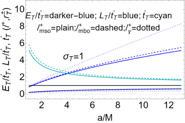
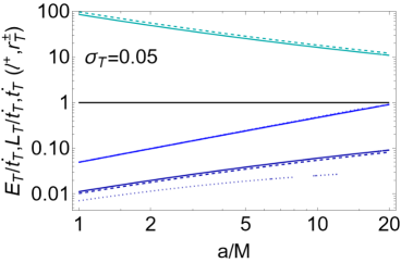
Figure 5: Analysis of the counter-rotating flows inversion points $r_{\mbox{\scriptsize{{T}}}}^{\pm}$ of Eq. (9) with fluid specific angular momentum $\ell^{+}<0$ of the plane $\sigma\equiv\sin^{2}\theta$, for different NS spin-mass ratios signed on the panels, where $\sigma=1$ is the equatorial plane. Notation $(mso)$ is for quantities evaluated on the marginally stable orbit, $(mbo)$ refers to the marginally bounded orbit, $(\gamma)$ indicates the marginally circular orbit. Particles energy ratio $\mathcal{E}_{\mbox{\scriptsize{{T}}}}/\dot{t}$ and angular momentum $\mathcal{L}_{\mbox{\scriptsize{{T}}}}/\dot{t}$ at the inversion points $r_{\mbox{\scriptsize{{T}}}}^{\pm}$ of Eqs (9) (where $u^{t}=\dot{t}$) are shown for two different inversion planes $\sigma_{\mbox{\scriptsize{{T}}}}$. (The most general solutions $r_{\mbox{\scriptsize{{T}}}}^{\pm}$ and $\sigma_{\mbox{\scriptsize{{T}}}}$ are shown not considering energy and momentum constraints of Sec. (III.2).)

The structure of this section is as follows:

In Sec. (III.2.1), we address the special case of inversion points from double tori systems orbiting NSs at equal fluid specific angular momentum. Tori and inversion points at $\ell=\pm a$ are explored in Sec. (III.2.2). Inversion points and torus outer edge are the focus of Sec. (III.2.3). The inversion point location in relation to the ergoregion in Sec. (III.2.4). In Sec. (III.2.5) the presence of double inversion points is discussed. Inversion points from proto-jets and the inversion points verticality are focused in Sec. (III.2.6). Some notes on the inversion coronas thickness and slow counter-rotating inversion spheres are in Sec. (III.2.7). Further notes on flows inversion points from orbiting tori are in Sec. (III.2.8). Relative location of the flows inversion points for different initial data and the existence of more inversion points for flow particle trajectory are investigated Sec. (B).

III.2.1 Double tori system

Slowly spinning NSs are characterized by the presence of double orbiting tori and also double cusped tori, distinguishing NSs from BHs, and having equal fluid specific angular momentum and therefore one common inversion radius $r_{\mbox{\scriptsize{{T}}}}^{\pm}(\sigma_{\mbox{\scriptsize{{T}}}})$. Such tori have been detailed in [44], for convenience we report below their main properties. The formation of this system in the geometries with $a\in]M,a_{2}[$ is due to the presence of fluids with $\ell^{-}<0$, and with $\ell^{-}>0$ and $\mathcal{E}<0$. Double tori can be both co-rotating or both counter-rotating.

More precisely, there are

(+,+)

Counter–rotating double toroids having $\ell^{-}=\ell^{+}<0$ orbiting NS with $a\in]a_{0},a_{2}[$—-Figs (6). The inner torus of the double system, centered in the ergoregion where $\mathcal{E}>0$ and $\mathcal{L}<0$, has $\ell^{-}\in\mathbf{L_{1}^{-}}$ and it can be cusped. The topology of outer counter-rotating torus depends on $\ell^{+}=\ell^{-}$ and the NS spin.

($-,-$)

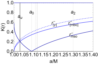
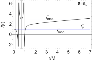
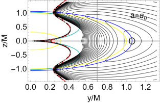
Figure 13: Analysis of the double co-rotating toroids with $\ell=\ell^{-}$, possible for $\ell>\ell_{mso}^{-}>0$ in $a\in]M,a_{0}[$. For $\ell^{-}>0$ inversion points are only for space-like particles with $(\mathcal{E}<0,\mathcal{L}<0)$ in the conditions of Sec. (C). Here the most general solutions $r_{\mbox{\scriptsize{{T}}}}^{\pm}$ are shown not considering the further constraints of Sec. (III.2). Spins $\{a_{0},a_{1},a_{2}\}$ are defined in Table (2) and $a_{u}=1.03M$. Notation $(mso)$ is for marginally stable orbit, $(mbo)$ is for marginally bounded orbit, $(\gamma)$ is for marginally circular orbit. Radius $r_{\epsilon}^{+}=2M$ is the outer ergosurface on the equatorial plane. Left panel: function $K(r)\equiv V_{eff}(\ell(r))$ ($V_{eff}$ is the fluid effective potential) as function of the spin $a/M$, evaluated for the radii of the extended geodetical structure. Center panel: fluid specific angular momentum $\ell(r)$ in the spacetime $a_{u}:K(r_{mso}^{-})=K(r^{-}_{[mbo]})$. Double co-rotating tori are possible for $\ell>\ell_{mso}^{-}$. Right panel: toroidal configurations in the geometry $a_{u}$ with specific angular momentum $\ell=1.025$. The proto-jets with cusp very close to the central singularity. There is $r=\sqrt{z^{2}+y^{2}}$ and $\theta=\arcsin y/\sqrt{z^{2}+y^{2}}$. Cyan curve is radius $r_{cr}=r_{\mbox{\scriptsize{{T}}}}^{+}=r_{\mbox{\scriptsize{{T}}}}^{-}$, defined in Eq. (10). Blue curve contains pressure maxima (the tori centers, dependent on $\ell$ only) and tori geometric maxima (dependent on $K$ and $\ell$), solutions of $\partial_{r}V_{eff}^{2}=0$ in the plane $(y,z)$, in this case it is $r=a^{2}$.

Co-rotating double toroids with $\ell^{-}>0$, orbiting NSs with $a\in]M,a_{0}[$, where $\mathcal{E}<0$ and $\mathcal{L}<0$ and $\ell>\ell_{mso}^{-}>0$. The inner torus of the couple can be cusped. As there is $\ell_{mso}^{-}>\ell_{\gamma}^{-}>0$, see Figs (7,8,13), the outer torus of the pair has $\ell\in\mathbf{L_{3}^{-}}$, and it is quiescent. There are only spacelike inversion points for $\mathcal{E}<0$ and $\mathcal{L}<0$.

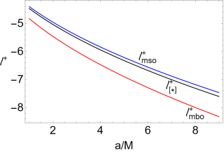
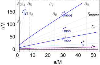
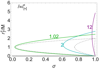
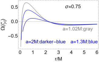
Figure 6: Inversion points for counter-rotating tori with fluid specific angular momentum $\ell=\ell^{+}<0$. The analysis for tori with fluid specific angular momentum $\ell^{-}$ is in Figs (15). Spins $\{a_{4},a_{5},a_{6},a_{7},a_{8},a_{9}\}$ are defined in Table (2). There is $\ell_{[*]}^{+}\equiv\ell^{-}(r_{[*]}^{+})$, and $r_{[*]}^{+}\equiv r_{mso}^{+}-(r_{mso}^{+}-r_{mbo}^{+})/2$. Upper left panel: fluid angular momentum $\ell_{[*]}^{+}$ and $\ell_{mso}^{+}$, $\ell_{mbo}^{+}$ (on the marginally stable and marginally bounded orbit respectively) as functions of the NS spin-mass ratio. Upper right panel: geodesic structure of the Kerr NS and the inversion radius $r_{\mbox{\scriptsize{{T}}}}$ for the torus model with center radius $r_{center}$ and cusp $r_{\times}$, where $\ell=\ell_{[*]}^{+}$. Bottom-left panel: inversion point radius $r_{\mbox{\scriptsize{{T}}}}^{\pm}$ as function of the plane $\sigma\equiv\sin^{2}\theta\in[0,1]$, for different NS spin-mass ratio signed on the curves for fluid specific angular momentum $\ell^{+}_{[*]}$. Dashed curves are the ergosurfaces $r_{\epsilon}^{\pm}$. Bottom right panel: analysis of the flows inversion points in terms of the relativistic angular velocities $\Omega$ for particles with fluid specific angular momentum $\ell=\ell_{[*]}^{+}$ for different spins. There is $\Omega(r_{\mbox{\scriptsize{{T}}}}^{\pm})=0$. Note the presence of two inversion points.

.

More in details:

(+,+): Double counter–rotating tori system with $\ell^{-}=\ell^{+}<0$

It is convenient to introduce the following spins.

$$a_{\iota}^{0}\equiv 1.1078:\ell^{+}_{\gamma}=\ell^{-}_{mso}<0,\quad a_{\iota}^{-}\equiv 1.1157:\ell^{+}_{mbo}=\ell^{-}_{mso}<0,\quad a_{\iota}^{+}\equiv 1.118M:\ell^{+}_{mso}=\ell^{-}_{mso}<0.$$ (11)

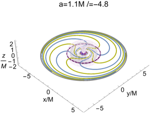
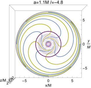
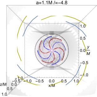
Figure 26: Test particle orbits with trajectories inversion points in the NS geometry with spin $a=1.1M$. The (counter-rotating) particle flows specific angular momentum is $\ell=-4.8$. There are two orbiting counter-rotating tori. In Figs (25) there is the analysis for the photons trajectories and description of the toroidal models. The initial radius is $r_{0}<r_{\times}$, where $r_{\times}$ is the torus inner edge. The inversion sphere $r_{\mbox{\scriptsize{{T}}}}$ is the light-purple surface. On the equatorial plane, radius $r_{\mbox{\scriptsize{{T}}}}^{\pm}$ is the purple curve. Gray surface is the geometry inner and outer ergosurfaces. Center panel is the above view of the left panel. Right panel is a close-up view of the center panel, where trajectories from the inner counter–rotating torus flow are shown.

(Note, there is $\ell_{mbo}^{-}>0$ for any spin $a>M$). Double tori with equal $\ell=\ell^{+}=\ell^{-}<0$, are in the geometries with $a<a_{\iota}^{+}$, for a selected range of specific angular momentum $\ell<0$–see Figs (19), Figs (25) and Figs (26).

Double cusped tori, can form in NSs spacetimes with $a<a_{\iota}^{+}$ with $\ell^{+}\in\mathbf{L_{1}^{+}}=]\ell_{mbo}^{+},\ell_{mso}^{+}[$ for cusped tori, or with, $\ell^{+}\in\mathbf{L_{2}^{+}}=]\ell_{\gamma}^{+},\ell_{mbo}^{+}[$ for tori and proto-jets, and quiescent tori in $\ell^{+}\in\mathbf{L_{3}^{+}}:\ell^{+}<\ell_{\gamma}^{+}$.

The situation is as follows:

–

For $a\in]a_{0},a_{2}[$, there is $\ell^{-}\in]\ell_{mso}^{-},0[$, and the double tori formation is constrained by $\ell_{mso}^{-}$, defining the limiting spins $\{a_{\iota}^{\pm},a_{0}\}$.

–

For $a\in]M,a_{0}[$, there is $\ell^{-}<0:\ell^{-}\in]-\infty,0[$ and double counter-rotating tori are always possible at $\ell^{-}<\ell_{mso}^{+}$. (The inner tori are always in $\mathbf{L_{1}^{-}}$ and entirely contained in the ergoregion).

In other words, for $a<a_{0}$, there is a very limited range for the inner tori center and cusp location, according to a variation of the momenta $\ell^{+}$ in $\mathbf{L_{1}^{+}},\mathbf{L_{2}^{+}}$ or $\mathbf{L_{3}^{+}}$. For $a<a_{0}$ there is $\ell_{mso}^{-}>0$, and co-rotating (cusped and quiescent) tori can be with $\ell>\ell_{mso}^{-}$. In these NS geometries, there still can be (cusped and quiescent) tori with $\ell^{-}<0$, having cusps in $r_{\times}\in]r_{0}^{-},r_{\delta}^{-}[$ and center in $r_{center}\in]r_{\delta}^{+},r_{0}^{+}[$.

More in details the situation is as follows:

–

For $a\in]a_{\iota}^{-},a_{\iota}^{+}[$, there is $\ell_{mso}^{-}\in]\ell_{mbo}^{+},\ell_{mso}^{+}[=\mathbf{L_{1}^{+}}$ (cusped tori).

–

For $a\in]a_{\iota}^{0},a_{\iota}^{-}[$, there is $\ell_{mso}^{-}\in]\ell_{\gamma}^{+},\ell_{mbo}^{+}[=\mathbf{L_{2}^{+}}$ (quiescent tori or proto-jets).

–

For $a\in]a_{0},a_{\iota}^{0}[$ there is $\ell_{mso}^{-}<\ell_{\gamma}^{+}$ and, in the range $\ell^{+}<\ell_{\gamma}^{+}$ ($\mathbf{L_{3}^{+}}$) (quiescent tori).

Note, for $a\in[a_{\iota}^{-},a_{\iota}^{+}]$ (there is $a_{\iota}^{-}>a_{0}$) there is $\ell_{mso}^{-}\in[\ell_{mbo}^{+},\ell_{mso}^{+}]$, and therefore in these geometries a double cusped tori system with $\ell\in]\ell_{mbo}^{+},\ell_{mso}^{-}[$ is possible. For $\ell^{-}=\ell^{+}<\ell_{\gamma}^{+}$, the outer disk is quiescent. For $\ell^{-}=\ell^{+}\in]\ell_{\gamma}^{+},\ell_{mbo}^{+}[$, the outer disk is quiescent, or there is a proto-jet. The inner torus of the couple is quiescent or cusped.

In the examples of Figs (17) we can see also the location of the inversion radius with respect to the ergosurfaces (further discussion on this aspect is in Sec. (III.2.4)).

($-,-$) Double co-rotating tori with $\ell^{-}>0$

There are no (time-like and photon-like) inversion points for $\ell=\ell^{-}>0$, however for completeness we also discuss co-rotating tori.

Double co-rotating tori can orbits NSs with spins $a\in]M,a_{0}[$, ($\mathcal{E}<0,\mathcal{L}<0$). The inner torus of the pair, having $\ell^{-}\in]\ell_{mso}^{-},+\infty[$, is always in $\mathbf{L_{1}^{-}}$. However, the outer torus is quiescent in $\mathbf{L_{3}^{-}}$, since $\ell_{mso}^{-}>\ell_{\gamma}^{-}$.

There is $0<\ell_{mbo}^{-}<\ell_{\gamma}^{-}=a<\ell_{mso}^{-}$. Quiescent tori with $\ell^{-}\in\mathbf{L_{3}^{-}}$ have center in $r_{center}>r_{[\gamma]}^{-}$ (inner edge is in $r>r_{0}^{+}$). As there are no solutions of $\ell(r)=\ell_{\gamma}^{-}=a$ in $]r_{\delta}^{-},r_{\delta}^{+}[$, therefore there are no double tori.

As noted in [44], there is $K(r_{[\gamma]}^{-})=\sqrt{1-{1}/{r_{[\gamma]}^{-}}}<1$, where $(r_{\gamma}^{-}=0,r_{[\gamma]}^{-}=a^{2})$ regulate the co-rotating proto-jets formation and define the range $\mathbf{L_{3}^{+}}\equiv\ell^{-}>\ell_{\gamma}^{-}=a$, where only quiescent tori are formed, where $r_{[\gamma]}^{-}$ is related to the light surfaces with frequency $\omega=1/\ell=1/a$. These limiting configurations have also a role in the case of tori with $\ell=0$, providing a case of toroidal GRHD (open) cusped configurations with "axial cusp"– [44]. The limiting case of $\ell=a$ is considered in Sec. (III.2.2).

Since $r_{\gamma}^{-}=0$, proto-jet cusps can be very close to the central singularity–see Figs (13) and Sec.(III.2.6).

More precisely: co-rotating proto-jets have cusps in $r_{j}\in]r_{\gamma}^{-},r_{mbo}^{-}[$, center in $]r_{[mbo]}^{-},r_{[\gamma]}^{-}[$ and momentum $\ell\in\mathbf{L_{2}^{-}}\equiv]\ell_{mbo}^{-},\ell_{\gamma}^{-}[$. The case of proto-jets emission is considered in details in and Sec.(III.2.6).

We summarize the situation as follows:

–

Tori couples orbiting in NSs with spin $a\in]M,a_{0}[$.

There is

$$r_{[mso]}^{-}>r_{[\gamma]}^{-}>r_{[mbo]}^{-}>r_{mso}^{-}>r_{mbo}^{-}>r_{\gamma}^{-}=0.$$ (12)

Radius $r_{[mso]}^{-}\equiv\tilde{r}_{[mso]}^{-}:\ell_{mso}^{-}\equiv\ell^{-}(r_{mso}^{-})=\ell(r)$, see Figs (1), regulates the outer co-rotating torus center location and constitutes a main difference with the BH geometry.

The outer torus is in $\mathbf{L_{3}^{-}}$, while the inner torus is in $\mathbf{L_{1}^{-}}\equiv\ell^{-}>\ell_{mso}^{-}>\ell_{\gamma}^{-}>\ell_{mbo}^{-}$. The outer torus cannot be cusped, as the center is located in $r>r_{[mso]}^{-}>r_{[\gamma]}^{-}>r_{[mbo]}^{-}$, and $\ell_{mso}^{-}>\ell_{mbo}^{-}$– Eqs (12).

The inner co-rotating tori, possible in the geometries with $a\in]M,a_{0}[$, where $\mathcal{E}<0$ and $\mathcal{L}<0$ and $\ell>\ell_{mso}^{-}>0$, have for very large $\ell^{-}$, inner edge stretching on $r_{\delta}^{-}$ (the center approaches $r_{\delta}^{+}$). The outer edge is studied in Sec. (III.2.3).

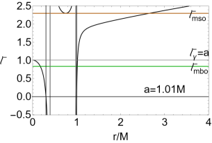
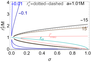
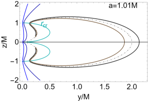
Figure 7: Double co-rotating tori system with fluid specific angular momentum $\ell=\ell^{-}$. Gray vertical lines are $r_{\delta}^{\pm}$, black vertical lines $r_{0}^{\pm}$. The specific angular momentum $\ell=\ell^{-}(r)$, the associated effective potentials $V_{eff}$ for NS spin-mass ratio $a=1.01M$ and $\ell^{-}$ according to the colour notations of the $\ell^{-}-r/M$ panels. The inversion points $r_{\mbox{\scriptsize{{T}}}}^{\pm}$ are also plotted as functions of the plane $\sigma=\sin^{2}\theta\in[0,1]$ (where $\sigma=1$ is the equatorial plane) for different $\ell$ signed on the curves. Here the most general solutions $r_{\mbox{\scriptsize{{T}}}}^{\pm}$ are shown not considering constraints of Sec. (III.2). For $\ell^{-}>0$ inversion points are only for space-like particles with $(\mathcal{E}<0,\mathcal{L}<0)$ in the conditions of Sec. (C). Radius $r_{\epsilon}^{\pm}$ is the outer and inner ergosurfaces, and $r_{cr}$ is defined in Eq. (10). Notation $(mbo)$ is for marginally bounded orbit, $(mso)$ for marginally stable orbit. Momentum $\ell_{\gamma}^{-}=a$ refers on the limiting value of the specific angular momentum $\ell=\ell^{-}>0$ for the occurrence of proto-jets (similarly to the $\ell^{+}$ case). There is $r=\sqrt{z^{2}+y^{2}}$ and $\sigma=y^{2}/(z^{2}+y^{2})$. The inversion sphere always closes on the equatorial plane, for small in magnitude $\ell$ closes at large $r$.

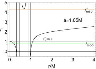
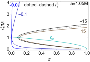
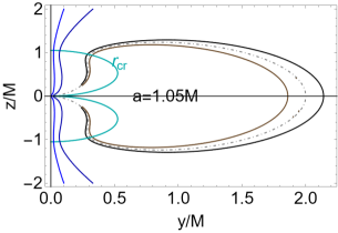
Figure 8: Double co-rotating tori system with fluid specific angular momentum $\ell=\ell^{-}$ for $a=1.05M$. See Figs (7).

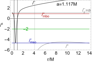
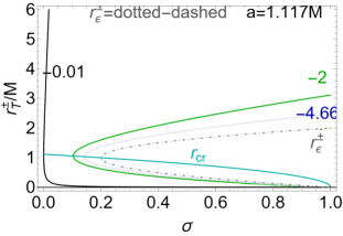
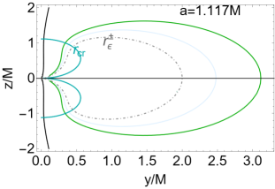
Figure 9: Double co-rotating tori system with fluid specific angular momentum $\ell=\ell^{-}$ for $a=1.117M$. See Figs (7).

From Figs (7) and (8) it is clear that for $a\in]M,a_{0}[$ there are double co-rotating tori only for $\ell>\ell_{mso}^{-}>\ell_{\gamma}^{+}=a>\ell_{mbo}^{-}$. The inner torus is cusped and is bounded by the light–surface with $\omega=1/\ell$. The outer torus of the couple is in $\mathbf{L_{3}^{-}}$ and therefore it is always quiescent and with center in $r>r_{[mso]}^{-}$.

For $\ell\in]\ell_{mbo}^{-},\ell_{\gamma}^{-}[=\mathbf{L_{3}^{-}}$ there are proto-jets or quiescent tori with cusp in $[0,r_{mbo}^{-}]$ and center in $[r_{[mbo]}^{-},r_{[\gamma]}^{-}]$. There are no double systems.

–

Tori in the NSs spacetimes with spin $]M,a_{2}]$.

In these spacetimes, the range $\ell\in[0,\ell_{mbo}^{-}]$ is a $\mathbf{L_{1}^{-}}$ range, where cusped and quiescent co-rotating tori are possible, with cusp in $[r_{mbo}^{-},r_{0}^{-}]$ and center in $[r_{0}^{+},r_{[mbo]}^{-}]$, including tori at $\ell=0$ with cusp in $r_{0}^{-}$ and center in $r_{0}^{+}$. The quiescent disk could have an inner edge in the regions bounded by $(r_{0}^{\pm},r_{\delta}^{\pm})$, where test circular particle orbits have $\mathcal{E}\gtrless 0$ and $\mathcal{L}<0$.

Inversion points for double systems with $\ell^{\pm}<0$

Tori in a double system with $\ell=\ell^{\pm}<0$ have same inversion spheres (determined by $\ell$), while generally proto-jets and accretion driven coronas are geometrically separated (there is $\ell_{mso}^{-}>\ell_{\gamma}^{-}$ at $a\in]M,a_{0}[$)– Sec. (III.2.6). On the other hand, only (particles and photons) flows with $\mathcal{E}>0$ and $\mathcal{L}<0$ have inversion points.

In the interpretation of the inversion sphere as accretion or proto-jets driven, the tori surfaces interaction with the inversion corona is relevant. In Sec. (III.2.3) this aspect is addressed in details.

For $\ell^{-}<0$, double counter-rotating tori are possible. Inner tori have cusp in $]r_{0}^{-},r_{\delta}^{-}[$ and center in $]r_{\delta}^{+},r_{0}^{+}[$, therefore torus includes the region $]r_{\delta}^{-},r_{\delta}^{+}[$. In this region cusped tori can exist with $\ell\in]\ell_{mso}^{+},+\infty[$. (Fluid effective potential is not well defined on the light surfaces $r_{s}$ with frequencies $\omega=1/\ell$ where the potential diverges. These surfaces constrain the torus edges).

Very large magnitude of fluid specific angular momentum

In this section we consider the case of $\ell^{\pm}$ very large in magnitude, focusing particularly on slowly spinning NSs with with $a\in]M,a_{0}[$. In these spacetimes, there are co-rotating and counter-rotating cusped tori ($\ell\in\mathbf{L_{1}^{-}}$) with $\ell\to\pm\infty$ (center and cusps close to the radii $r_{\delta}^{\pm}$ where $\ell=\pm\infty$), with centers bounded by $]r_{mso}^{+},r_{\delta}^{+}[$ (co-rotating fluids) and $]r_{\delta}^{+},r_{0}^{+}[$ (counter-rotating fluids) and cusps in $]r_{\delta}^{-},r_{mso}^{-}[$ (co-rotating fluids) and $]r_{0}^{-},r_{\delta}^{-}[$ (counter-rotating fluids).

Tori with $\ell=\ell^{-}<0$ and $\mathcal{L}<0$ are only in the geometries $]a_{0},a_{2}[$– Figs (7),(8) ,(9). In the limits $\ell\to\pm\infty$, there is $r_{\mbox{\scriptsize{{T}}}}^{\pm}=r_{\epsilon}^{\pm}$ and $\sigma_{\mbox{\scriptsize{{T}}}}=\sigma_{erg}$. The inversion sphere approaches the ergosurfaces from above, in the counter-rotating case, (and from below for the co-rotating case for space-like particles, implying that the counter-rotating sphere is larger than the co-rotating inversion sphere). The counter-rotating inversion spheres decrease with the angular momentum magnitude, (while it increases with $\ell^{-}>0$), bounded by $r_{\epsilon}^{\pm}$. The outer torus of a pair with $\ell^{+}\to-\infty$ (and with $\ell^{-}\to+\infty$) are quiescent tori in $\mathbf{L^{+}_{3}}$ ( $\mathbf{L_{3}^{-}})$, centered very far from the central singularity.

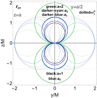
Figure 22: Radius $r_{cr}$ of Eq. (10), in the plane $(y,z)$ where $r=\sqrt{z^{2}+y^{2}}$ and $\sigma\equiv\sin^{2}\theta=y^{2}/(z^{2}+y^{2})$. It is $y=\pm\sqrt{z(\mp a-z)}$ and $z=\pm\frac{1}{2}\left(\pm\sqrt{a^{2}-4y^{2}}+a\right)$, for different spins signed on the panels. Dashed gray lines are $y=a/2$ and $z=a$. Radii $r_{\epsilon}^{\pm}$ are the outer and inner ergosurfaces. Notation $(mso,mbo,\gamma)$ refers the marginally stable, marginally bounded and last circular orbit respectively.

The inversion spheres for $\ell\to\pm\infty$ are similarly approaching from below and above the ergosurfaces respectively–Figs (7) and (8). (An interesting case is represented by the solution $u^{\phi}=0$ for very small $\ell^{-}<0$ in magnitude. For the cusped tori with $\ell^{-}\in]-\infty,0[$ (with cusp in $]r_{0}^{-},r_{\delta}^{-}[$), the smaller in magnitude the fluid specific angular momentum is the larger the sphere (see Figs (22) for the relative analysis of $r_{cr}$).)

Therefore: in the spacetimes with $a\in]a_{0},a_{2}[$ double cusped counter-rotating configurations can exist for $\ell^{-}\in]\ell_{mso}^{-},\ell_{mso}^{+}[$.

Inner cusped torus of the couple has momentum $]\ell_{mso}^{-},\ell_{mbo}^{-}[$ ($\mathbf{L_{1}^{-}}$ range). The cusp is located in $]r_{0}^{-},r_{mso}^{-}[$ while the center in $]r_{mso}^{-},r_{0}^{+}[$ (there is $\ell^{-}<0$), or otherwise the cusp in $]r_{mbo}^{-},r_{0}^{-}[$ and center in $]r_{0}^{+},r_{[mbo]}^{-}[$ (with $\ell^{-}>0$). We include also tori at $\ell=0$, with critical points of pressure in $r_{0}^{\pm}$.

For $\ell\in]\ell_{mbo}^{-},\ell_{\gamma}^{-}[$, there are only proto-jets with cusps in $]0,r_{mbo}^{-}[$. For $\ell^{-}>\ell_{\gamma}^{-}=a$, there are quiescent tori (this is an $\mathbf{L_{3}^{-}}$ range) with center in $r>r_{[\gamma]}^{-}=a^{2}$–see Figs (9). Inversion points are all outside the ergoregion.

For very small momenta magnitude $\ell\leq 0$, there are counter-rotating tori with $\ell=\ell^{-}\neq\ell^{+}$ in $\mathbf{L_{1}^{-}}$. In this case the inversion coronas, for accretion driven flows, is very large and located out of the ergoregion.

However the inversion sphere is always a closed surface (there is always a inversion point on the equatorial plane). (Further constrains to the inversion points due to the conditions $(\mathcal{E},\mathcal{L})$ constant on the flow particles are not considered.).

For $\ell=\ell^{+}$ the largest inversion sphere is at $\ell_{mso}^{+}$ for $a\lessapprox M$, discussed in more details in Sec. (III.2.6). The maximal extension on the equatorial plane is studied in [44].

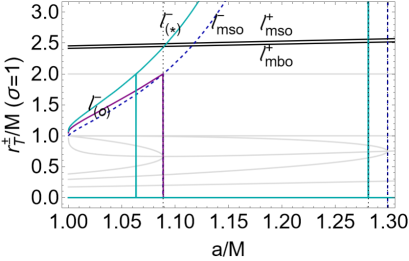
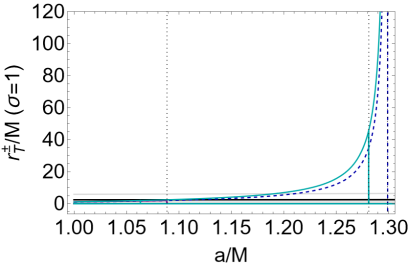
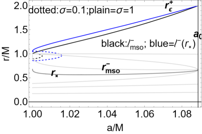
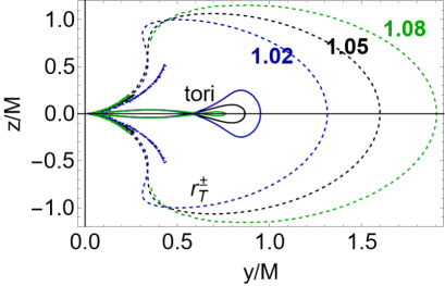
Figure 10: Upper line: Inversion radius $r_{\mbox{\scriptsize{{T}}}}^{\pm}$ on the equatorial plane $\sigma=1$ as function of the NS spin-mass ratio $a/M$. (The most general solutions $r_{\mbox{\scriptsize{{T}}}}^{\pm}$, further constraints are in Sec. (III.2).) Gray curves are the Kerr NS geodesic structure. The inversion radius is evaluated on different flow specific angular momenta $\ell$, signed on the curves. For $\ell^{-}>0$ inversion points are only for space-like particles with $(\mathcal{E}<0,\mathcal{L}<0)$ in the conditions of Sec. (C). Left panel is a close-up view of the left panel. There is $\ell_{(o)}^{-}\equiv\ell^{-}(r_{(o)}^{-})$ where $r_{(o)}^{-}\equiv r_{mso}^{-}-(r_{mso}^{-}-r_{\delta}^{-})/2$, while $\ell_{(*)}^{-}\equiv\ell^{-}(r_{(*)}^{-})$ where $r_{(*)}^{-}\equiv r_{mso}^{-}-(r_{mso}^{-}-r_{0}^{-})/2$. Radius $r_{mso}^{-}$ is the marginally stable orbit for fluids with specific angular momentum $\ell^{-}$, on $r_{0}^{-}$ there is $\mathcal{L}=\ell=0$ (test particle circular angular momentum and fluid momentum), on $r_{\delta}^{-}$ there is $\mathcal{E}=0$ (energy of test particle circular orbits). $\ell_{mso}^{+}<0$ and $\ell_{mbo}^{+}<0$ are the specific angular momenta for fluid with $\ell=\ell^{+}<0$ on the marginally stable orbit and marginally bounded orbit respectively. Bottom left panel: light-gray curves are the geodesic structure for $a<a_{0}$, blue and black curves are the inversion radius for particle flows with $\ell=\ell_{mso}^{-}>0$ and $\ell^{-}(r_{\times})>0$ signed on the panels. Radius $r_{\epsilon}^{+}=2M$ is the outer ergosurface on the equatorial plane. Bottom right panel: tori (plain curves) and inversion points (dashed curves) for selected values of the NS spin-mass ratios $a/M$ signed on the panels, according to the tori models of the left panel. There is $r=\sqrt{z^{2}+y^{2}}$ and $\sigma\equiv\sin^{2}\theta=y^{2}/(z^{2}+y^{2})$.

In Figs (10) solutions with $\ell=\ell^{-}>0$ are studied, where $\mathcal{E}<0$ and $\mathcal{L}<0$ at $a\in]M,a_{0}[$ (spacelike, tachyonic particles inversion points), and $\ell=\ell^{-}<0$ with $\mathcal{E}>0$, $\mathcal{L}<0$ at $a\in]a_{0},a_{2}[$. By increasing the spin, the inversion point sphere widens, extends outwards, and increases the vertical height. The associated torus, on the other hand, shrinks, and approaches the central singularity, having an inner Roche lobe much larger than the outer Roche lobe. The case of very low $\ell^{-}\in]\ell_{mso}^{+},0[$ will be detailed in Sec. (III.2.6).

III.2.2 Tori and inversion points at $\ell=\pm a$

Here we consider inversion points with $\ell=\pm a$ and tori with $\ell=-a$. There are no double tori systems for $\ell=\pm a$. We can details the situation as follows

Tori with $\ell=a$.

There are no double tori with $\ell=a$ as $\ell_{mso}^{-}>\ell_{\gamma}^{-}=a$ for $a\in]M,a_{0}[$ – Figs (13).

More precisely for $\ell=\ell^{-}=\ell_{\gamma}^{-}=a$ there are (quiescent tori or) proto-jets with cusp approaching the central singularity (there is $r_{\gamma}^{-}=0$) and with on center in $r_{[\gamma]}^{-}=a^{2}\in]r_{[mbo]}^{-},r_{[mso]}^{-}[$. In the NS with $a<a_{0}$, tori with $\ell^{-}>0$ have inner edge in $]r_{\delta}^{-},r_{mso}^{-}[$ and center $]r_{mso}^{-},r_{\delta}^{+}[$.

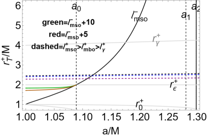
Figure 12: Analysis of the inversion radius $r_{\mbox{\scriptsize{{T}}}}^{+}$ on the equatorial plane $\sigma=1$, for fluids with specific angular momentum $\ell=\ell^{+}<0$ and $\ell=\ell^{-}\gtreqless 0$ signed on the panel, as functions of the NS spin-mass ratios $a/M$. Spins $\{a_{0},a_{1},a_{2}\}$ are defined in Table (2). Notation $(mso)$ is for marginally stable orbit, $(mbo)$ is for marginally bounded orbit, $(\gamma)$ is for marginally circular orbit. The most general solutions are shown not considering constraints of Sec. (III.2).)

There are no inversion points for $\ell=a$, since $\ell=\ell^{-}=a>0$ in $r=\{0,r_{[\gamma]}^{-}\}$ and, on $r_{[\gamma]}^{-}$ there is $\mathcal{L}>0$(spacelike inversion radius increases with $\ell>0$, bounded from above by the ergosurfaces–Figs (7)– there is $r_{\mbox{\scriptsize{{T}}}}>r_{out}$–Figs (12).

Tori with $\ell=-a$

We distinguish the two cases $\ell=\ell^{\pm}=-a$ respectively.

–

Tori with $\ell=\ell^{+}=-a$ can form in the geometries with $a>a_{a}^{-}=2\left(\sqrt{2}+2\right)M\approx 6.828M$ as cusped tori, quiescent tori or proto–jets according to the NS spins–Figs (11).

–

Tori with $\ell=\ell^{-}=-a$ can form only in the spacetimes with $a\in]M,a_{t}[$, where $a_{t}\equiv 2\left(2-\sqrt{2}\right)M\approx 1.17157M$, there are quiescent or cusped tori, with cups bounded by $r_{0}^{-}$ and $r_{\delta}^{-}$ or $r_{mso}^{-}$, and centers bounded by $r_{0}^{+}$ and $r_{\delta}^{+}$ or $r_{mso}^{+}$, according to the NS spin–Figs (11).

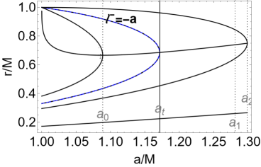
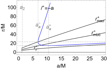
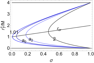
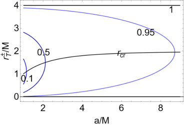
Figure 11: Analysis of the tori (upper line) and flow inversion points (bottom line) with $\ell=-a$. There is $a_{t}\equiv 2\left(2-\sqrt{2}\right)M$, $a_{a}^{+}\equiv 2\sqrt{2}\left(\sqrt{3}+2\right)M$ and $a_{a}^{-}\equiv 2\left(\sqrt{2}+2\right)M$–see Eqs (13). There is $\sigma=\sin^{2}\theta\in[0,1]$ (equatorial plane is $\sigma=1$). Bottom line, inversion radius at $\ell=-a$ as function of $\sigma$ for different $a$ signed on the curves (left) and as function of $a$ for different $\sigma$ (right). Upper line: critical points of pressure for tori with $\ell^{-}=-a$ (left) and $\ell^{+}=-a$ (right). Black curves are the geodesic structures. Spins $\{a_{0},a_{1},a_{2}\}$ are defined in Table (2).

Inversion points with $\ell=-a$

There are inversion points for $\ell=-a$ for

$$r_{\mbox{\scriptsize{{T}}}}^{\pm}\in]0,4M]:\quad(\sigma=1,r_{\mbox{\scriptsize{{T}}}}^{+}=4M),(\sigma_{\mbox{\scriptsize{{T}}}}^{S},r_{\mbox{\scriptsize{{T}}}}=r_{S}^{-}),(\sigma\in]\sigma_{\mbox{\scriptsize{{T}}}}^{S},1[,r_{\mbox{\scriptsize{{T}}}}=r_{S}^{\pm}),\quad\mbox{where}$$ (13)

$$\sigma_{\mbox{\scriptsize{{T}}}}^{S}\equiv\frac{1}{2}\left[a\sqrt{a^{2}+8}-(2+a^{2})\right],\quad r_{S}^{\pm}\equiv\sigma+1\pm\sqrt{a^{2}(\sigma-1)+(\sigma+1)^{2}},\quad r_{cr}=\frac{a}{2}\left[\sqrt{a^{2}+8}-a\right]$$

increasing with the spin and the plane–Figs (11) (there is $r_{cr}(\sigma)=1+\sigma$).

The analysis of the inversion point location with respect to the outer edge is done in Sec. (III.2.3)

III.2.3 Inversion points and torus outer edge

Here we explore the inversion spheres and the location of the flow inversion points on the equatorial plane with respect to the tori outer edge.

There can be, in a fixed spacetime region, more orbiting configurations with different $\ell$–see for example[45, 26, 46, 47, 48, 49]. In this case, all proto-jets and cusped configurations have equal inversion coronas respectively, depending only on the NS spin $a/M$.

The inversion corona is in general a narrow region surrounding the central singularity. As the conora thickness is generally small, inversion points location in the corona vary little with $\ell$ in the range of values defining the corona . The inversion radius can be on the equatorial plane at $r_{\mbox{\scriptsize{{T}}}}<r_{\times}$ (or $r_{J}$), and this is always the case for tori–driven and proto-jets driven configurations with $\ell=\ell^{+}<0$ in Figs (19) and (18,17), or otherwise the corona can also "embed" the inner torus of a couple with with $\ell=\ell^{-}$, for example in Figs (19,18,16,10)). Inversion corona is interpreted as accretion or proto-jets driven if, on the equatorial plane, $r_{\mbox{\scriptsize{{T}}}}<r_{\times}$ or $r_{\mbox{\scriptsize{{T}}}}<r_{J}$. On planes different from the equatorial, the situation depends on the particles initial conditions on the orbiting structure, on the jet collimation angle, on the torus morphological characteristics, as its height on the equatorial plane.

We can use the concept of "excretion" inversion points if $r_{\mbox{\scriptsize{{T}}}}>r_{\times}$ on the equatorial plane which is the case for tori with $\ell^{-}<0$ (at $a\in]M,a_{2}[$). Fluids with $\ell=\ell^{+}$ have always accretion or proto-jets driven inversion points on the equatorial plane i.e. $2M=r_{\epsilon}^{+}<r_{\mbox{\scriptsize{{T}}}}<r_{\gamma}^{+}$. (However, we stress that there is no "external cusp" or "extraction process" associated with the cusp, as for example emerges in the models of thick discs analyzed in contexts in which there is a toroidal magnetic field, in the presence of a cosmological constant or electric charge[55, 56, 57, 57, 58, 2005PhRvD..71b4037S]. Here the term excretion distinguishes the case where an accretion driven or proto-jets driven interpretation is possible from the case where the inversion sphere or a portion of the inversion sphere embeds the torus or is external with respect to the central singularity.).

A further aspect to be analysed is the location of the inversion point, on the equatorial plane, in relation with the torus outer edge. The cusped tori outer edge (maximum outer torus extension on the equatorial plane) is provided in [44] with $K=V_{eff}(r_{\times},\ell)$ (where the cusp is $r_{\times p}$ for $a\in]a_{0},a_{1}[$, and $r_{\times}$ for $a\in]a_{1},a_{2}[$. (In Figs (14) we prove that, for $\ell^{-}\lessgtr 0$, there is $r_{outer}<r_{\mbox{\scriptsize{{T}}}}$, the tori outer edge is always inside the ergoregion.).

In NSs with $a\leq a_{2}$, the co-rotating and counter-rotating cusped tori outer edge never crosses the ergosurface on the equatorial plane. (Tori are also confined by the light surface with $\omega=1/\ell$.) Counter-rotating tori orbiting NS with $a<a_{2}$ can cross the radius $r_{0}^{+}$ for certain values of the specific angular momentum and NS spin. For co-rotating tori in the NSs spacetimes with $a<a_{0}$, with centers and cusps bounded by $r_{0}^{\pm}$ and $r_{\delta}^{\pm}$, the outer edge can cross $r_{0}^{+}$ or $r_{\delta}^{-}$.

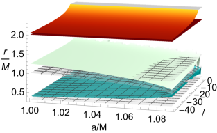
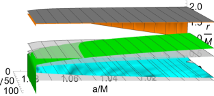
Figure 14: Analysis of the outer edge $r_{out}$ of the tori orbiting NSs with spins $a\in]M,a_{2}]$ with centers and cusps bounded by $r_{0}^{\pm}$ and $r_{\delta}^{\pm}$. Panels show the cusped torus inner and outer edges and the inversion point $r_{\mbox{\scriptsize{{T}}}}^{+}$ on the equatorial plane. There is $r_{\times}<r_{out}<r_{\mbox{\scriptsize{{T}}}}^{+}$. There is no solution $r_{out}=r_{\epsilon}^{+}=2M$ on the equatorial plane. Radius $r_{\epsilon}^{+}$ is the outer ergosurface (gray-plane). Light-gray surfaces are $r_{0}^{\pm}$ and $r_{\delta}^{\pm}$. Spins $\{a_{0},a_{1},a_{2}\}$ are defined inTable (2). Left panel: counter-rotating tori. Note the inversion radius is always out of the ergoregion, the outer edge is inside the ergoregion crossing, for some $(a,\ell)$, the plane $r_{0}^{+}$. Center panel: co-rotating tori. The inversion radius is always inside the ergoregion. Right panel: counter-rotating tori. The inversion radius is located out of the ergoregion.

III.2.4 Inversion points inside and outside the ergoregion

In this section we explore inversion points location with respect to the geometry ergoregion. For $a\in]M,a_{2}]$, counter-rotating tori in the ergoregion are possible. For counter-rotating fluids, inversion points are only out of the ergoregion –Eqs (31). (Contrary to the counter-rotating case, inversion points with $\ell>0$, possible only for spacelike tachyonic–particles with $\mathcal{L}<0$ and $\mathcal{E}<0$, in the geometries with $a\in]0,a_{0}]$, exist only in the ergoregion at $r\in]r_{\epsilon}^{-},r_{\epsilon}^{+}[$–see also Eqs (27)).

Tori in the ergoregion

We consider tori with momentum $\ell=\ell^{-}\lesseqgtr 0$ in the NSs ergoregion. There are, for $a\in]M,a_{0}[$, co-rotating cusped tori in the ergoregion. There are also larger tori with cusp in the ergoregion at $[r_{0}^{-},r_{mbo}^{-}]$. Proto-jets and co-rotating tori cusps are in the ergoregion, in $]r_{\gamma}^{-},r_{mbo}^{-}[$ and $[r_{0}^{-},r_{mbo}^{-}]$ respectively.

Let us introduce the spins $\{a_{mso},a_{mbo}\}$ defined as:

$$a_{mso}\equiv 2.828M:\bar{r}_{mso}^{-}=2M\quad\mbox{and}\quad a_{mbo}\equiv 4.828M:r_{mbo}^{-}=2M.$$ (14)

For $a\in]a_{2},a_{mso}[$, proto-jets and co-rotating cusps are only in the ergoregion. For $a\in]a_{mso},a_{mbo}[$, tori cusps are out of the ergoregion and proto-jets cusps are inside the ergoregion. For $a>a_{mbo}$, proto-jets and tori cusps are out of the ergoregion–see Figs (15) and Figs (1).

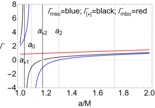
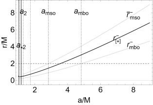
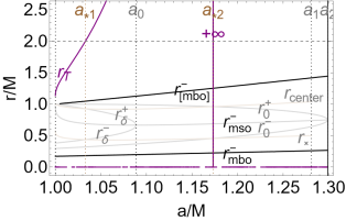
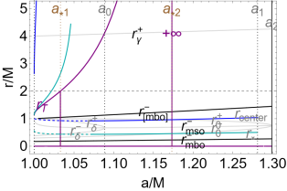
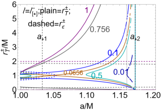
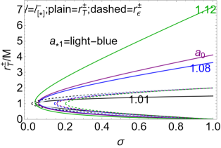
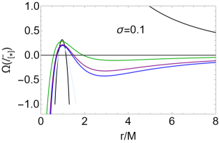
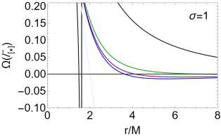
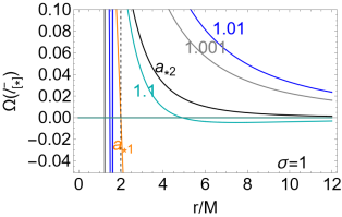
Figure 15: Inversion points for flows with fluid specific angular momentum $\ell^{-}$. For $\ell^{-}>0$ inversion points are only for space-like particles with $(\mathcal{E}<0,\mathcal{L}<0)$ in the conditions of Sec. (C). The most general solutions $r_{\mbox{\scriptsize{{T}}}}^{\pm}$ are shown not considering constraints of Sec. (III.2). Spins $\{a_{0},a_{1},a_{2}\}$ are defined in Table (2). Spins $\{a_{*1},a_{*2}\}$ are defined in Eqs (15), spins $\{a_{mso},a_{mbo}\}$ are defined in Eqs (14). There is $\ell_{[*]}^{-}\equiv\ell^{-}(r_{[*]}^{-}),\quad r_{[*]}^{-}\equiv r_{mso}^{-}-(r_{mso}^{-}-r_{mbo}^{-})/2$. Upper left panel: fluid angular momentum $\ell_{[*]}^{-}$ and $\ell_{mso}^{-}$, $\ell_{mbo}^{-}$ (on the marginally stable and marginally bounded orbit respectively) as functions of the NS spin-mass ratio. Upper Center panel: geodesic structure of the Kerr NS and radius $r_{[*]}^{-}$ as function of $a/M$. Upper right panel and center-line left panel show the inversion radius $r_{\mbox{\scriptsize{{T}}}}$ (on the equatorial plane) for the torus model with center radius $r_{center}$ and cusp $r_{\times}$, where $\ell=\ell_{[*]}^{-}$. Center-line right and center panels:: inversion point radius $r_{\mbox{\scriptsize{{T}}}}^{\pm}$ for different planes $\sigma\equiv\sin^{2}\theta\in[0,1]$ ($\sigma=1$ is the equatorial plane), signed on the curves, as function of spin-mass ratio $a/M$ (center panel) and as function of the plane, for different NS spin-mass ratio signed on the curves (right panel) for fluid specific angular momentum $\ell^{-}_{[*]}$. Note the location of the inversion radius with respect to the ergosurfaces $r_{\epsilon}^{\pm}$ (dashed curves). Bottom line panel: analysis of the flows inversion points in terms of the relativistic angular velocities $\Omega$ evaluated for particles with fluid specific angular momentum $\ell=\ell_{[*]}^{-}$ for different plane sigma $\sigma$ and spins as signed on the planes (left and right panels) according to notation of the center-line right-panel. There is $\Omega(r_{\mbox{\scriptsize{{T}}}}^{\pm})=0$. Bottom right panel shows $\Omega(\ell_{[*]}^{-})$ on the equatorial plane $(\sigma=1)$ for different spins $a/M$ signed on the curves. Note the presence of two inversion points for each curve at $\sigma<1$. The analysis for the counter-rotating tori with fluid specific angular momentum $\ell=\ell^{+}<0$ is in Figs (6).

From Figs (15) it is clear how, in the regions where $\ell_{mso}^{-}>0$ with $\mathcal{L}<0$, there is $\ell_{mso}^{-}>\ell_{mbo}^{-}$ at $a<a_{0}$.

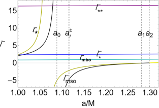
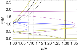
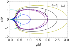
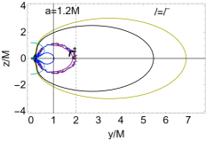
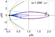
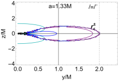
Figure 16: Analysis of tori with fluids specific angular momentum $\ell=\ell^{-}$, $\ell^{-}=\ell^{+}<0$ and flows inversion points. For $\ell^{-}>0$ inversion points are only for space-like particles with $(\mathcal{E}<0,\mathcal{L}<0)$ in the conditions of Sec. (C). Here most general solutions $r_{\mbox{\scriptsize{{T}}}}^{\pm}$ are shown, while further constraints are in Sec. (III.2). Spins $a_{\iota}^{\pm}$, are defined in Eqs (11). There is $a_{\mu}\equiv a_{\iota}^{+}-(a_{\iota}^{+}-a_{\iota}^{-})/2$, and $(\ell_{*}^{-},\ell_{**}^{-})$ are $\ell_{*}^{-}\equiv\ell_{mbo}^{-}+1.5$, $\ell_{**}^{-}\equiv\ell_{mbo}^{-}+15.5$, with $\ell_{\star}^{-}\equiv\ell^{-}(r_{\star}^{-})$, where $r_{\star}^{-}\equiv\bar{r}_{mso}^{-}-(\bar{r}_{mso}^{-}-r_{mbo}^{-})/9$, for $a>a_{1}$, and $r_{\star}^{-}\equiv\bar{r}_{mso}^{-}-(\bar{r}_{mso}^{-}-r_{0}^{-})/2$ for $a\in]M,a_{1}[$. (mso is for marginally stable orbit and mbo is for marginally bounded orbit). See also Figs (25), Figs (26). Upper line left panel: the fluid specific angular momentum $\ell^{-}$ as function of $a/M$. Radii $r_{\epsilon}^{\pm}$ are the outer and inner ergosurfaces. Upper line right panel is a close up view of the center panel: inversion radius $r_{\mbox{\scriptsize{{T}}}}^{\pm}$ on different planes $\sigma\equiv\sin^{2}\theta$, on the equatorial plane $\sigma=1$ (plain curves) and $\sigma=0.5$ (dashed curves) and specific angular momenta according to the colors notation of the left panel. Remaining panels show the inversion radius $r_{\mbox{\scriptsize{{T}}}}^{\pm}$ on the plane $(y/M,z/M)$, where $\sigma=\sin^{2}\theta={y^{2}}/({z^{2}+y^{2}})$ and $r=\sqrt{z^{2}+y^{2}}$, for different fluid specific angular momenta $\ell$, according to the notation signed on the upper line left panel. Tori models and accretion flows inversion points are shown in Figs (18) and Figs (19). Note the inversion radius location with respect to the ergosurface $r_{\epsilon}^{\pm}$. Figs (17) show the analysis for fluids with momenta $\ell=\ell^{+}<0$. Radius $r_{cr}=r_{\mbox{\scriptsize{{T}}}}^{+}=r_{\mbox{\scriptsize{{T}}}}^{-}$ is defined in Eq. (10).

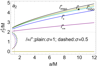
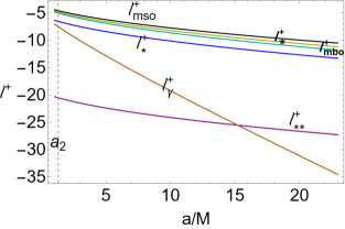
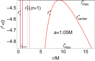
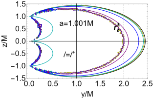
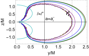
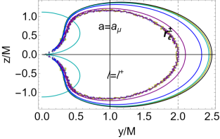
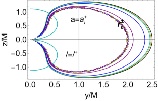
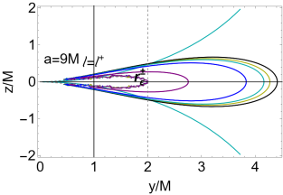
Figure 17: Tori with fluids specific angular momentum $\ell^{+}<0$ and $\ell^{-}=\ell^{+}<0$ and flows inversion points. (The most general solutions $r_{\mbox{\scriptsize{{T}}}}^{\pm}$ are shown, discussion on the constraints are in Sec. (III.2).) Spins $a_{\iota}^{\pm}$ are defined in Eqs (11). Radius $r_{cr}=r_{\mbox{\scriptsize{{T}}}}^{+}=r_{\mbox{\scriptsize{{T}}}}^{-}$ is defined in Eq. (10). There is $a_{\mu}\equiv a_{\iota}^{+}-({a_{\iota}^{+}-a_{\iota}^{-}})/{2}$, and the fluid specific angular momenta $(\ell_{*}^{+},\ell_{**}^{+})$ are $\ell_{*}^{\pm}\equiv\ell_{mbo}^{+}\mp 1.5$, $\ell_{**}^{\pm}\equiv\ell_{mbo}^{+}\mp 15.5$. There is $\ell_{\star}^{+}\equiv\ell^{+}(r_{\star}^{+})$, where $r_{\star}^{+}\equiv\bar{r}_{mso}^{+}-(\bar{r}_{mso}^{+}-r_{mbo}^{+})/1.25$. Radii $r_{\epsilon}^{\pm}$ are the outer and inner ergosurfaces. Upper left panel: inversion radius $r_{\mbox{\scriptsize{{T}}}}^{\pm}$ on different planes $\sigma\equiv\sin^{2}\theta$ and specific angular momenta signed on the panel. (mso is for marginally stable orbit and mbo is for marginally bounded orbit). Upper center panel: specific angular momenta as functions of $a/M$. Upper right panel: specific angular momentum $\ell^{\pm}<0$ as function of $r/M$ for the NS spin $a=1.05M$. Remaining panels show the inversion radius $r_{\mbox{\scriptsize{{T}}}}^{\pm}$ on the plane $(y/M,z/M)$, where $\sigma=\sin^{2}\theta={y^{2}}/({z^{2}+y^{2}})$ and $r=\sqrt{z^{2}+y^{2}}$, for different fluid specific angular momenta $\ell$, according to the notation signed on the upper line left panel. Tori models and accretion flows inversion points are shown in Figs (18) and Figs (19). Note the inversion radius location with respect to the ergosurfaces $r_{\epsilon}^{\pm}$. Figs (16) show the analysis for fluids with momenta $\ell=\ell^{-}$.

Inversion points: inner and outer tori

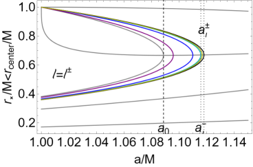
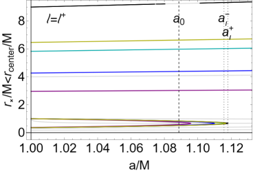
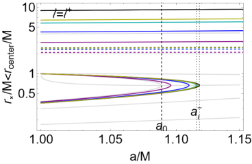
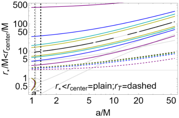
Figure 18: Gray curves are the NS geodesic structure. Spin $a_{0}$ is defined in Table (2) and spins $a_{\iota}^{\pm}$ in Eqs (11.) The center and inner edge of cusped tori $r_{center}>r_{\times}$ (plain curves) and the flow inversion point $r_{\mbox{\scriptsize{{T}}}}$ (dashed curves), on the equatorial plane $\sigma=1$ are shown as functions of the NS spin–mass ratio for different fluid specific angular momentum according to the colors notation of Figs (17). (Here the most general solutions $r_{\mbox{\scriptsize{{T}}}}^{\pm}$ are shown not considering explicitly the constraints of Sec. (III.2).) Tori configurations are shown in Figs (19). It is clear the presence of double tori configurations.

For $\ell=\ell^{+}$ there is $r_{\times}>r_{\gamma}^{+}>r_{\mbox{\scriptsize{{T}}}}^{+}$ on the equatorial plane, and $r_{\mbox{\scriptsize{{T}}}}^{+}$ can be interpreted as accretion driven inversion point on the equatorial plane–Figs (18). The distance cusps-inversion points increases with the NS spins, for tori with cusp at $r>r_{\gamma}^{+}$, and approaches the central singularity increasing $\ell^{+}$ in magnitude.

In the double counter-rotating tori system with $\ell^{-}=\ell^{+}<0$ for $a<a_{\iota}^{+}$, there is one inversion point on the equatorial plane, and for the inner smaller torus of the double system (having $\ell<0$ with $\mathcal{L}<0$ and $\mathcal{E}>0$) it can be interpreted as "excretion" driven inversion point (in the sense of Sec. (III.2.1)), or for particle flows incoming from the outer region at $\ell$ constant, with general $u^{\phi}$. On planes different from the equatorial there are two inversion points, the inner one can be interpreted as accretion driven inversion point. Therefore, in the case of a double system, the inner region of the inversion corona, might be considered the more active part, in the sense that particles from different flows converge with equal $\ell$ from the external tori (the flow crosses the outer inversion point) and from the inner torus accretion flows (particles can also have different $u^{\phi}$ [44]). Consequently, the observation of the inversion point could provide indication of the orbiting structures.

We have inferred that tori with $\ell^{-}<0$ have no accretion driven inversion point on the equatorial plane. It is simple to see, in the case $\ell^{-}<0$, as the inversion points are always out of the ergoregion, while the cusps are always inside the ergoregion. For $a\in]M,a_{0}[$ it has been proved that, while $r_{\times}\in]r_{\delta}^{-},\tilde{r}_{mso}^{-}[$, there is $r_{\mbox{\scriptsize{{T}}}}^{+}>r_{0}^{+}>r_{\times}$. Accretion driven interpretation is still possible for planes different from the equatorial, where there is a inversion point "internal" to the cusp, and therefore a particle coming from the disk towards the central singularity has a inversion radius. The inversion radius external to the torus (outer to the outer edge) can play a role in the flux forming the torus or for poorly collimated jets. These counter-rotating tori are much smaller than the inversion sphere, and this could imply that the detection of particles (and photons) at the inversion sphere can be a tracer for the orbiting structures which are limited at $\ell\in]0,\tilde{\ell}_{mso}^{-}]$–(see the situation for $a<a_{0}$ and $r_{\times}\in]r_{\delta}^{-},\tilde{r}^{-}_{mso}[$).

As clear from Figs (17), the inversion corona from counter–rotating accretion tori is a narrow region with maximum thickness on the equatorial plane.

For $a\gtrapprox 1$ the corona inner part differs from for fast and slowly spinning central attractors. In Figs (26) double inversion points re showed, and the possibility of in-falling or out-going particles crossing the inversion sphere.

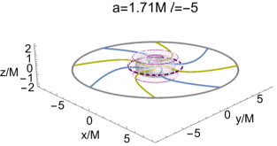
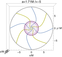
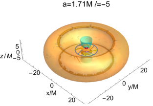
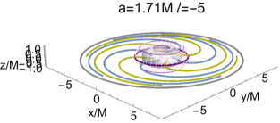
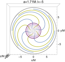
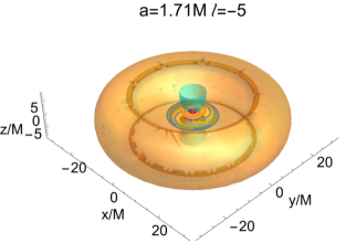
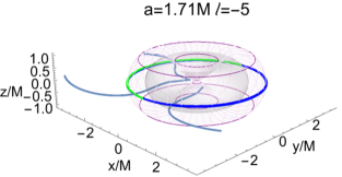
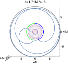
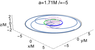
Figure 27: Photons orbits (upper line) and test particle orbits (center line) with trajectories inversion points the NS geometry with spin $a=1.71M$. The specific angular momentum is $\ell=-5$. The initial radius is $r_{0}<r_{\times}$, where $r_{\times}$ is the torus inner edge. The inversion sphere $r_{\mbox{\scriptsize{{T}}}}$ is light-purple surface. On the equatorial plane radius $r_{\mbox{\scriptsize{{T}}}}^{\pm}$ is the purple curve. Gray surface is the geometry inner and outer ergosurfaces. Upper and center line: Center panel is the above view of the right panel. Right panel shown the torus (orange surface) while the green surface is the light surface with rotational frequency $\omega=1/\ell$. Bottom line: Test particles analysis where $\theta_{0}=\pi/2$ and Carter constant is $Q=0.0035$.

As clear from Figs (25,27), the outer torus can also be larger than the inversion corona. The accretion driven coronas can also be rather small–Figs(19). As these tori are generally geometrically thick tori orbiting very strong attractors, associated to high accretion rates, the small region of the inversion corona might be a very active part of the accretion flows. (The inner disk of a double counter-rotating toroids with $\ell=\ell^{+}=\ell^{-}<0$, the inner Roche lobe can be larger than the torus outer Roche lobe and the disk is smaller of the "embedding" inversion sphere–Figs (17) and Figs (16).).

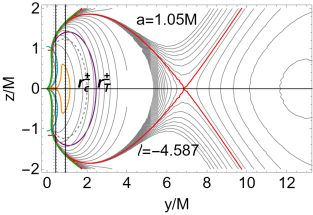
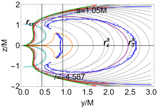
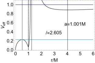
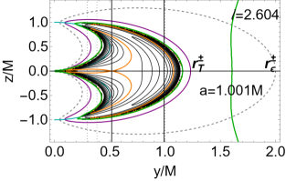
Figure 19: Inversion spheres in double tori systems.Tori effective potential for different spins and fluid specific angular momentum as signed on the panels. The tori centers and cusps are also signed with vertical lines. It is clear the presence of an orbiting double tori systems. Tori configurations and the inversion points $r_{{\mbox{\scriptsize{{T}}}}}^{\pm}$ are shown in the plane $(y/M,z/M)$ where $\sigma=\sin^{2}\theta={y^{2}}/({z^{2}+y^{2}})$ and $r=\sqrt{z^{2}+y^{2}}$ for different fluid specific angular momenta $\ell$. (The most general solutions $r_{\mbox{\scriptsize{{T}}}}^{\pm}$ and $\sigma_{\mbox{\scriptsize{{T}}}}$ are shown, while discussion on the constrains is in Sec. (III.2).) Note the inversion radius location with respect to the ergosurface $r_{\epsilon}^{\pm}$. For $\ell^{-}>0$ inversion points are only for space-like particles with $(\mathcal{E}<0,\mathcal{L}<0)$ in the conditions of Sec. (C). The limiting boundary configuration for the inner torus is the defined by the light surface $r_{s}$ with frequency $\omega=1/\ell$ (darker-green surface)–See also Figs (18) and Figs (17).

Example

If $\mathcal{E}>0$, the inversion radius is outside of the ergoregion (there is $\mathcal{L}<0$ and $\ell<0$). For $\ell>0$ there are no inversion point but spacelike inversion point for $(\mathcal{E}<0,\mathcal{L}<0)$ in the ergoregion (for $s=-1$). Let us consider below the more general solution $r_{\mbox{\scriptsize{{T}}}}^{\pm}$.

In the example considered in Figs (6)–Figs (15), we introduced the spin functions $\{a_{*1},a_{*2}\}$, and the fluid specific angular momenta and radii $(\ell_{[*]}^{\pm},r_{[*]})$:

$$a_{*2}\equiv 1.173M:\{r_{center}=r_{0}^{+},r_{\times}=r_{0}^{-}\},\quad a_{*1}\equiv 1.03297M:\{r_{center}=r_{\delta}^{+},r_{\times}=r_{\delta}^{-}\},$$ (15)

$$\ell_{[*]}^{\pm}\equiv\ell^{\pm}(r_{[*]}),\quad r_{[*]}\equiv r_{mso}^{\pm}-\frac{r_{mso}^{\pm}-r_{mbo}^{\pm}}{2}.$$

In Figs (15), solutions $r_{\mbox{\scriptsize{{T}}}}$ are only for $a<a_{*2}$, as there is $r_{center}^{-}<r_{0}^{+}$ and therefore $\mathcal{L}<0$. The inversion point is inside the ergoregion for $a<a_{*1}$, where $r_{center}<r_{\delta}^{+}$ and $\mathcal{L}<0$ with $\mathcal{E}<0$–see also Figs (3,4,17,19,25).

Inversion points $r_{\mbox{\scriptsize{{T}}}}$ for fluids with specific angular momentum $\ell^{-}$ are only in the geometries with spins $a\in]M,a_{*2}[$, where $\mathcal{L}<0$ and there is $\ell^{-}\gtreqless 0$ (according to the sign of $\mathcal{E}$). At $a=a_{2}$ there is the limiting condition $r_{{\mbox{\scriptsize{{T}}}}}\to\infty$ on the equatorial plane.

The discriminant spin $a_{*1}$ determines the classes of NSs according to the location of the inversion points with respect to the ergosurface. (Note that spins $\{a_{*1},a_{*2}\}$ are defined according to the geodetic properties on the equatorial plane.). For $a>a_{*1}$, the inversion point is out of the ergoregion ($r>r_{\epsilon}^{+}$), viceversa for $a<a_{*1}$, the inversion point is inside the ergoregion. Some tori orbiting geometries $a<a_{*1}$ are co-rotating (with $\mathcal{L}<0$ and $\mathcal{E}<0$), while for $a\in]a_{*1},a_{*2}[$, tori are counter-rotating with $\mathcal{L}<0$ and $\mathcal{E}>0$. For $a>a_{*2}$ there are co-rotating tori with $\mathcal{L}>0$ and $\mathcal{E}>0$ (with no inversion point), and counter-rotating tori with $\mathcal{L}<0$.

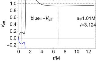
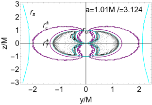
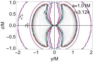
Figure 20: NS geometry with spin $a=1.01M$. The (co-rotating) particle flows specific angular momentum is $\ell=3.124$. The most general solutions $r_{\mbox{\scriptsize{{T}}}}^{\pm}$ are shown not considering constraints of Sec. (III.2). For $\ell^{-}>0$ inversion points are only for space-like particles with $(\mathcal{E}<0,\mathcal{L}<0)$ in the conditions of Sec. (C). The initial radius is $r_{0}<r_{\times}$, where $r_{\times}$ is the torus inner edge. The inversion sphere $r_{\mbox{\scriptsize{{T}}}}$ is purple surface. Left panel show the effective potential for the orbiting torus. Dotted curves show the location of torus cusp $r_{\times}$. Note that at $\ell=3.124$ there are two classes of tori, the inner class admits a cusped torus, the outer class has no cusp. Center panel: equi–density surfaces are shown, the cyan curve is the light surface $r_{s}$ with rotational frequency $\omega=1/\ell$. Radius $r_{\epsilon}^{\pm}$ is the geometry ergosuface. Radius $r_{cr}=r_{\mbox{\scriptsize{{T}}}}^{+}=r_{\mbox{\scriptsize{{T}}}}^{-}$ is defined in Eq. (10). Right panel is a close-up view of the center panel on the torus.

From the analysis of Figs (25,26,27,10) it is clear that the inversion point can be directly related to the outer torus flows (even in the condition $\ell^{-}>0$ with $\mathcal{L}<0$, for tachyonic particles), for $\ell^{-}<0$, where there is also the case $\ell^{-}=\ell^{+}<0$. In the determination of the double inversion point, the limiting role represented by the outer horizon for the BH geometries is played by the radius $r_{cr}$ for the NSs, which also determines the distancing of the inversion point from the central axis of rotation and differentiates slow rotating NSs from faster spinning NSs –see Figs (16).

III.2.5 On the double inversion points

A distinctive characteristic of the NS geometries with respect to the BH geometries is the presence of two inversion point functions $r_{\mbox{\scriptsize{{T}}}}^{\pm}(\sigma_{\mbox{\scriptsize{{T}}}})$ for fixed $\sigma\neq 1$, therefore from $u^{\phi}\lessgtr 0$ and $u^{\phi}\gtrless 0$ at constant $\ell$ and double inversion points at fixed $\ell$ and vertical coordinate $z_{\mbox{\scriptsize{{T}}}}$–Figs (3),(4)– Figs (16,17,19,20,25).

In the BH spacetime this characteristic is limited to fast spinning BHs, depending on the fluid specific angular momentum and far from the equatorial plane. A double inversion point in the BH spacetime occurs in $]z(+),z_{\mbox{\scriptsize{{T}}}}^{\max}[$ and $]r_{+},y(+)[$ where $z_{\mbox{\scriptsize{{T}}}}^{\max}$ is the maximum vertical coordinate of the inversion sphere and $z(+):r_{+}$ and $y(+):z=r_{+}$, where $r_{+}$ is the BH outer horizon and the coordinates are as follows $r=\sqrt{z^{2}+y^{2}}$ and $\sigma=\sin^{2}\theta=y^{2}/(y^{2}+z^{2})$ [15].

The inversion corona is the same for particles and photons, but distinguishes co-rotating from counter-rotating fluids and it is different for accretion-driven and proto-jets driven flows. Function $r_{\mbox{\scriptsize{{T}}}}^{\pm}(\sigma_{\mbox{\scriptsize{{T}}}})$ defines a (regular) locus of points surrounding the central singularity, where there can be two inversion points for each plane $\sigma\neq 1$. The values $(r_{\mbox{\scriptsize{{T}}}},\sigma_{\mbox{\scriptsize{{T}}}})$, constrained on the inversion sphere $r_{\mbox{\scriptsize{{T}}}}^{\pm}(\sigma_{\mbox{\scriptsize{{T}}}})$, is fixed by the particles (photons) trajectory. In Figs (6) and Figs (15) is the analysis of the relativistic angular velocity $\Omega$, showing two inversion radii $r_{{\mbox{\scriptsize{{T}}}}}^{\pm}$ at fixed $\ell$ and plane $\sigma_{\mbox{\scriptsize{{T}}}}$. In Sec. (B) the relative location of inversion points according $\ell$ was considered. Defining the inner and outer inversion point (at fixed $\sigma_{\mbox{\scriptsize{{T}}}}$ and $\ell$) as $r_{{\mbox{\scriptsize{{T}}}}}^{(i)}<r_{\mbox{\scriptsize{{T}}}}^{(o)}$ respectively, there is $\Omega<0$ for $r<r_{{\mbox{\scriptsize{{T}}}}}^{(i)}\cup r>r_{\mbox{\scriptsize{{T}}}}^{(o)}$, and $\Omega>0$ for $r\in]r_{{\mbox{\scriptsize{{T}}}}}^{(i)},r_{{\mbox{\scriptsize{{T}}}}}^{(o)}[$.

III.2.6 Proto-jets driven inversion points and inversion points verticality

We conclude this work considering in Sec. (III.2.6), proot-jets driven inversion points and, in Sec. (III.2.6), the inversion point location with respect to the singularity rotational axis (verticality of the inversion point).

Inversion points from proto-jets Fluids with momentum $\ell=\ell^{+}$ form proto-jets with $\ell\in\mathbf{L_{2}^{+}}\equiv]\ell_{\gamma}^{+},\ell^{+}_{mbo}[$. Fluids with $\ell=\ell^{-}$ form proto-jets $\ell\in\mathbf{L_{2}^{-}}\equiv]\ell_{mbo}^{-},\ell_{\gamma}^{-}[$, where $\ell_{mbo}^{-}>0$ and $\ell_{\gamma}^{-}=a>0$.

Radii $r_{mbo}^{-}>r_{\gamma}^{-}=0$, constraint the critical points of pressure for fluids with $\mathcal{E}>0$ and $\mathcal{L}>0$ ($\ell=\ell^{-}>0$), with a proto-jet cusp in $r_{j}\in]0,r_{mbo}^{-}]$ and center in $r_{center}\in]{r}_{[mbo]},r_{[\gamma]}^{-}[$, where $r_{[\gamma]}^{-}=a^{2}$– see Figs (1). Therefore proto-jets with $\ell=\ell^{-}$ are always co-rotating and there are no inversion points for proto-jets driven flows with $\ell=\ell^{-}$.

Proto-jets driven inversion points exist only for fluids with $\ell=\ell^{+}<0$ with a cusp out of the ergoregion at $r_{j}\in]r_{\gamma}^{+},r_{mbo}^{+}[$, and centers in $r\in[r_{[mbo]}^{+},r_{[\gamma]}^{+}]$)–Figs (1). Proto-jets driven inversion coronas are out of the ergoregion and bounded by the values $]\ell^{+}_{mbo},\ell^{+}_{\gamma}[$. Proto-jets inversion points are distinguishable from accretion inversion points. Compared with accretion driven coronas, proto-jets driven coronas are closer to the ergoregion, approaching the equatorial plane, and smaller in extension with larger thickness. Increasing the spin, the corona maximum point (verticality) moves far from the attractor (the inversion radius always decreases with increasing $\ell^{+}<0$ in magnitude). Inversion points verticality Inversion point verticality (vertical coordinate $z_{\mbox{\scriptsize{{T}}}}$, elongation on the central rotational axis of the inversion point) is particularly relevant for proto-jet driven configurations.

In Figs (21) inversion points location with respect to the central rotational axis is shown.

Figure 21: Analysis of the inversion point verticality for fluids with specific angular momentum $\ell=\ell^{+}<0$ (left panel) and $\ell=\ell^{-}$ (center and right panels). Here the most general solutions $r_{\mbox{\scriptsize{{T}}}}^{\pm}$ are shown not considering constraints of Sec. (III.2). For $\ell^{-}>0$ inversion points are only for space-like particles with $(\mathcal{E}<0,\mathcal{L}<0)$ in the conditions of Sec. (C). Inversion radius $r^{\pm}_{\mbox{\scriptsize{{T}}}}(\ell)$ is plotted for selected values of $\ell$ and NS spins $a/M$, signed on the panel, in the plane $(y,z)$ where $r=\sqrt{z^{2}+y^{2}}$ and $\sigma\equiv\sin^{2}\theta=y^{2}/(z^{2}+y^{2})$. Spin $a=M$ is the extreme Kerr BH. Radii $r_{\epsilon}^{\pm}$ are the outer and inner ergosurfaces. Notation $(mso,mbo,\gamma)$ refers the marginally stable, marginally bounded and last circular orbit respectively. Purple surface in the center panel is focused on the right panel.

Radius $r_{cr}$, defined in Eqs (10), provides an indication on the inversion radius maximum extension. Radius $r_{cr}$, is related to the $r_{\mbox{\scriptsize{{T}}}}^{\pm}$ definition, and it is a background property dependent on the spin $a$ only, and therefore describes both fluid particles and photons. (The inversion radius does not depend on the particles radial velocity and therefore is relevant also for outgoing particles–see for example Figs (27)).

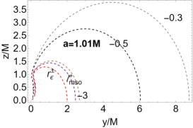
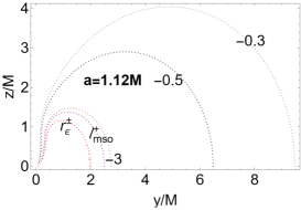
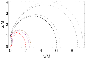
Figure 23: Analysis of the inversion sphere for low angular momenta counter-rotating tori $\ell^{-}\in]\ell_{mso}^{+},0[$ in the ergoregion of NSs with $a\in[0,a_{2}]$. There is $r=\sqrt{z^{2}+y^{2}}$ and $\sigma\equiv\sin^{2}\theta=y^{2}/(z^{2}+y^{2})$. I Radii $r_{\epsilon}^{\pm}$ are the outer and inner ergosurfaces. Notation $mso$ refers the marginally stable circular orbit, $mbo$ to marginally bounded orbit and $(\gamma)$ to the marginally circular orbit. Upper left panel: purple surface is the inversion sphere at specific angular momentum $\ell^{-}=-3.5>\ell_{mso}^{-}$. Black lines are test particles ingoing trajectories crossing the inversion spheres and out–going trajectory crossing the inversion sphere. Gray region is the ergosurfaces orange region is the counter-rotating torus in the ergoregion. Upper center and right panel: specific angular momenta $\ell^{\pm}<0$ as functions of $r/M$ for selected spins signed on the panel. Gray lines are $\ell_{mso}^{\pm}$ and $(\ell_{mbo}^{+},\ell_{\gamma}^{+})$. Below left and center panel, the ergosurfaces and inversion spheres for selected values of $\ell<0$ signed on the curves and for the NSs spins reported on the panels. Bottom right panel shows super-imposition of the left and center plots.

Inversion corona approaches the ergoregion as $\ell$ increases in magnitude.

The situation for flows with $\ell=\ell^{+}$ is clear: the maximum of the inversion point verticality $z_{\mbox{\scriptsize{{T}}}}^{\max}$, occurs for $\ell=\ell_{mso}^{-}$ and $a\approx M$,and there is (for proto-jets and accretion driven flows) $z_{\mbox{\scriptsize{{T}}}}^{\max}<1.4M$–Figs (17).

For proto-jets and accretion driven flows, the corona is larger the smaller the momenta magnitude is, and the smaller NS spin is. Increasing the spin and decreasing in magnitude $\ell$, the inversion coronas extend on the equatorial plane. Furthermore, at $y<y_{\mbox{\scriptsize{{T}}}}^{max}$, the proto-jets and accretion driven coronas are very close and with narrow thickness, reducing approximately to an orbit.

Let us consider now the more general solution $\ell_{\mbox{\scriptsize{{T}}}}=\ell^{-}$. For $\ell=\ell^{-}$ the situation is more complex. Inversion points exist only for accretion driven flows in NSs with $a\in]M,a_{2}[$. In $a=a_{2}$, with $\mathcal{L}<0$, there is a limiting situation, where for $a\leq a_{2}$ the inversion sphere for $\ell=\ell^{-}<0$ (and $\mathcal{L}<0$) increases in extension on the equatorial plane and on the vertical direction becoming, in the limit $a=a_{2}$ (where $\ell=0$), asymptotically large and therefore on the NS poles–Figs (15).

The inversion sphere is inside or outside the ergoregion according to $\ell=\ell^{-}>0$ (space-like particles) or $\ell=\ell^{-}<0$–see discussion in Eqs (15).

For $\ell=\ell_{mso}^{\pm}$, increasing the spin, the verticality decreases.

For $\ell=\ell^{+}$ the inversion sphere becomes slender and on the equatorial plane moving far from the attractor.

At $\ell=\ell_{mso}^{-}<0$, increasing the spin, the spheres (and the verticality) always increase. (Note that there are tori with $\ell^{-}\neq\ell^{+}<0$.) (Inversion spheres for $\ell^{-}<0$ are larger than the inversion spheres for $\ell^{-}>0$ (spacelike solutions for tachyons), as the counter-rotating ones contain in the ergoregion, while the co-rotating spheres are inside the ergoregion– Figs (8,7, 9)).

(The inversion sphere maximum for $\ell^{-}>0$ is provided by the ergoregion, to which the inversion sphere tends for large $a$ (i.e. $a\leq a_{0}$) and for $\ell^{-}\to+\infty$, occurring for critical points of pressure close to $r_{\delta}^{\pm}$. These tori are cusped and located inside the ergoregion. They belong to a double toroidal system with equal $\ell^{-}>0$ (where $\ell_{mso}^{-}>\ell_{\gamma}^{-}$). The outer co-rotating torus has $\ell\in\mathbf{L_{3}^{-}}$, it is quiescent and with center in $r>r_{[mso]}^{-}>r_{[\gamma]}^{-}>r_{[mbo]}^{-}$ and geometrically separated from the inner torus–see Figs (24).

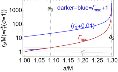
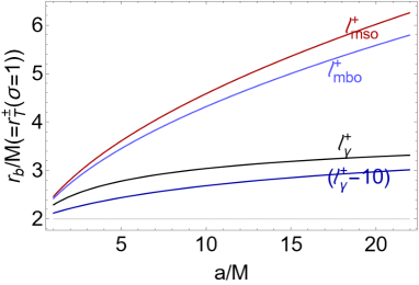
Figure 24: Maximal extension on the equatorial plane of the inversion radius $r_{\mbox{\scriptsize{{T}}}}^{\pm}=r_{b}$ for fluids with specific angular momentum $\ell^{-}$ (left panel) and $\ell^{+}<0$ (right panel). Notation $(mso)$ refers to marginally stable orbit, $(mbo)$ to marginally bounded orbit, $\gamma$ to the last circular orbit, at $r_{0}^{\pm}$ there is $\ell=0$. For $\ell^{-}>0$ inversion points are only for space-like particles with $(\mathcal{E}<0,\mathcal{L}<0)$ in the conditions of Sec. (C). Spins $\{a_{0},a_{1}\}$ are defined in Table (2).

III.2.7 Inversion coronas thickness and slow counter-rotating spheres

We conclude this section with some final comments on the coronas thickness and on slow counter-rotating spheres with $\ell^{-}\in]\ell_{mso}^{+},0[$. Let us consider Figs (21) and (23).

For $\ell^{+}$, the accretion coronas thickness is always smaller then the proto-jets coronas thickness and decreases, approaching the singularity and the rotational axis, increasing on the equatorial plane. The inversion corona is therefore a particular active region close to the NS. The thickness increases with the NSs spins, increasing also the thickness differences between the accretion driven and proto-jets driven coronas.

The slow momenta inversion spheres, located out of the ergoregion, are not immediately related to flows coming from the counter-rotating tori in the ergoregion of NSs with $a\in[M,a_{2}]$ (especially on the equatorial plane). There is no inversion corona for these, quiescent or cusped, tori as the specific momentum is in $\mathbf{L_{1}^{-}}=]\ell_{mso}^{+},0[$.

As expected, the inversion sphere increases, decreasing the momentum in magnitude and it is always closed (there is always a inversion point on the equatorial plane).

It should be noted that a solution $r_{\mbox{\scriptsize{{T}}}}^{\pm}$ (not related to tori) also exists for $a>a_{2}$ (with $\mathcal{E}>0$ and $\mathcal{L}<0$). It is interesting to note that there are always inversion points for very large distances from the NS, not linked to the frame dragging of the ergoregion, and there are also solutions for BH spacetimes.

The inversion spheres verticality is very high for very small $\ell$ in magnitude, however here we do not consider this case as it is not related to the orbiting tori.

Interestingly in general, increasing the NS spin, the inversion sphere increases, contrary to the case of high momenta in magnitude, where it decreases with the NS spin, as for the case $\ell=\ell^{+}<\ell_{mso}^{+}$.

III.2.8 Flow inversion points from orbiting tori

Inversion spheres are fixed by the tori specific angular momentum. We assume tori fix the initial conditions on the (free) fluid particles trajectories, in terms of energy (for timelike particles inherited by the torus parameter $K$) and momentum ($\ell=$constant), considering the (unstable) circular orbit at $r_{\times}$ (or $r_{0}\leq r_{\times}$) as torus inner edge, and time–like particle energy as $K$ (at $r_{\times}$) fixed by the torus. The reliability of this assumption is confronted by the small variation of the (narrow) inversion coronas thickness with the initial data (parameter $\ell=$constant) variation and by the inversion points independence on flow initial data (other than the specific angular momentum)– Figs (4).

In the analysis of Figs (17,18,19) and Figs (25) double tori were considered.

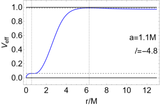
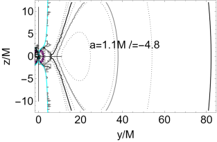
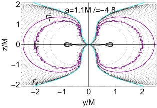
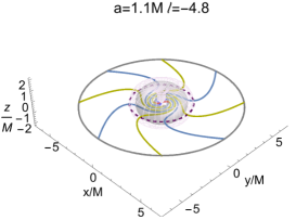
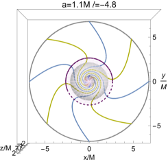
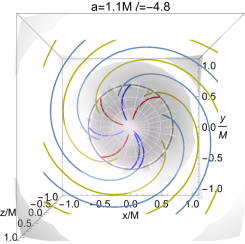
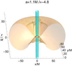
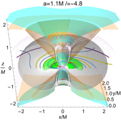
Figure 25: Photon orbits with trajectories inversion points in the NS geometry with spin $a=1.1M$. The (counter-rotating) particle flows specific angular momentum is $\ell=-4.8$. There are two orbiting counter-rotating tori with $\ell^{-}=\ell^{+}=-4.8$. In Figs (26) there is the analysis for the test particles trajectories. The initial radius is $r_{0}<r_{\times}$, where $r_{\times}$ is the torus inner edge (cusp). The inversion sphere $r_{\mbox{\scriptsize{{T}}}}$ is the light-purple surface. On the equatorial plane radius $r_{\mbox{\scriptsize{{T}}}}^{\pm}$ is the purple curve. Upper line: left panel shows the effective potential for the system of two counter–rotating tori. Dotted curves show the location of tori cusps $r_{\times}$. Center panel: equi–density surfaces an outer torus, cyan curve is the light surface with rotational frequency $\omega=1/\ell$. Right panel is a close-up view of the center panel on the inner torus. Radius $r_{\epsilon}^{\pm}$ is the geometry ergosuface. Center line: Gray surface is the geometry inner and outer ergosurfaces. Center panel is the above view of the left panel. Right panel is a close-up view of the center panel, where trajectories from the inner counter-rotating torus flow are shown. Bottom panels show the outer torus (orange surface) and inner torus (green surface), while the cyan surface is the light–surface with rotational frequency $\omega=1/\ell$. Right panel is a close-up view of the left panel.

Flows with $\ell=\ell^{-}<0$ can be interpretable, for the outer torus of the pair at $\ell^{-}=\ell^{+}<0$, as accretion or proto-jets driven inversion points. A distinctive property of Kerr NS geometries is the presence of two inversion radii at planes different from the equatorial– discussed in more details in Sec. (III.2.5). The inversion point is uniquely defined by the $\ell$ and, at fixed $\ell$, there can be two (sphere) radii $r_{\mbox{\scriptsize{{T}}}}^{\pm}(\sigma)$, defining a closed inversion sphere. Viceversa, functions $r_{\mbox{\scriptsize{{T}}}}^{\pm}(\sigma)$ correspond to one $\ell$. The inversion point does not explicitly depend on the orbital energy of the particle (or photon) or on the torus topology (if quiescent or cusped), which is fixed by the $K$ parameter (related to the energy definition $\mathcal{E}$).

In Figs (19), a limiting closed configuration is shown bounding the inner torus of a couple with momentum $\ell^{-}$, orbiting in the NS ergoregion, identified with the light surfaces $r_{s}$ solutions for the null-like circular orbits with rotational frequencies $\omega_{\pm}=1/\ell:{g}(\mathcal{L},{\mathcal{L}})=0$, defined from the Killing vector $\mathcal{L}=\xi^{t}+\omega\xi^{\phi}$. The limiting frequencies $\omega_{\pm}$ bound the (time-like) stationary observers four-velocity, (where, in the BH spacetimes, $\omega_{\pm}(r_{\pm})=\omega_{H}^{\pm}$ are the frequencies of the outer and inner Kerr horizons respectively). There is $\omega_{\pm}(r\to 0)=1/a$, where $r_{\gamma}^{-}=0$ and $\ell_{\gamma}^{-}=0$.

IV Final Remarks

The inversion points have been analyzed for accretion driven and proto-jets driven flow in the Kerr super-spinar background. Defined by the condition $u^{\phi}=0$, the flow inversion points are related to the orbiting structures defining accretion driven and proto-jets driven inversion coronas.

The location of inversion points has been considered also in relation to the ergoregion, characterizing the dragging effects on the accretion flows and jet emission in Kerr super-spinars and proving that NSs are distinguished from the BHs by the presence of double inversion points on planes different from the equatorial.

In accretion and jet driven flows, possible strong observational signatures of these attractors, are highlighted. Our results prove that inversion points can constitute an observational aspect capable of distinguishing the super-spinars.

The flow carries in fact information about the accretion structures around the central attractor. These structures are governed by the balance of the hydrodynamic and centrifugal forces and also effects of super-spinars repulsive gravity. In this paper we addressed in particular the special case of double tori with equal specific angular momentum and slow counter-rotating inversion spheres, tori and inversion points for $\ell=\pm a$ and excretion driven inversion points. Finally proto-jets driven inversion points and inversion points verticality have been discussed focused in relation to the inversion coronas thickness. (On the other hand, for slow tori with $\ell^{-}\in]\ell_{mso}^{+},0[$, inversion spheres verticality is very high for very small $\ell$ in magnitude, this case however is not related to the orbiting tori.). With narrow thickness and small extension on the equatorial plane and rotational central axis, the inversion surface varies little with the fluid initial conditions and the details of the emission processes. The inversion coronas, including all the possible inversion surfaces, are a geometric property of the background. Therefore the information provided by the analysis of the inversion points has a remarkable observational significance and applicability to various orbiting toroidal models.

In these different scenarios our analysis provides distinguishable physical characteristics of jets and accretion tori for possible strong observational signature of the primordial Kerr superspinars. Therefore this work is part of the research on the possible observational evidences of Kerr naked singularity solutions, and the astrophysical tracers distinguishing black holes from their super-spinar counterparts having cosmological relevance (as predicted for example by string theory [59]). However the observational properties in the inversion coronas we expect depend strongly on the processes timescales i.e. the time flow reaches the inversion points, depending on the initial data.

The accretion and proto-jets flows are constituted by particles and photons, coming from toroids orbiting a central Kerr super-spinar. Constraints on the accretion or proto-jets driven flows are grounded on the assumption that the accretion disk "inner edge" is located between marginally bounded orbit and marginally stable orbit for the accretion driven flow and marginally stable and marginally circular orbit for the proto-jets driven flows (with the exception for inner tori in the ergoregion with $a\in]M,a_{2}[$), translated into the range of values of the $\ell$ parameter defining the coronas. The closed surfaces, defining inversion coronas are spherical shells, fixed by the fluids specific angular momentum, where the particles and photons flow toroidal velocity is null. The inversion corona surround the central singularity, distinguishing co-rotating and counter-rotating flows from proto-jets and accretion driven flows. (Co-rotating flows ($a\ell>0$) have no (timelike or photon like particle) inversion points. However, in Sec. (C) we also focused on the $\ell>0$ case with $\mathcal{E}<0$ and $\mathcal{L}<0$, where spacelike (tachyonic particles) inversion points are possible inside the ergoregion, in relation to tori orbiting a very small region of the ergoregion of certain slowly spinning NSs. Further notes on the co-rotating flows inversion points in relation to the NS causal structure are in Sec. (C).) We deepen the analysis in Sec. (B) discussing in detail the relative location of the inversion points in accreting flows.

The results of this analysis are also based on the possibility to relate the flow inversion points to the orbiting configurations, differentiated in accretion and proto-jets structures, defining the driven and proto-jets driven flows respectively. In each case we distinguish the definition and properties of the inversion coronas.

The special case of double tori with equal specific angular momentum is a notable example of a trace for the presence of a center super-spinar in contrast with a central BH attractor. A further remarkable feature is the existence of tori for specific angular parameter $\ell=\pm a$ and the inversion points of their flows. We also discussed the existence of excretion driven inversion points due to the repulsive gravity effects typical of the ergoregions of a super-spinars class. More in general we focused on the location of inversion points in relation to the ergoregion and with the respect to the torus outer edge, relevant for the double orbiting systems at equal $\ell$ in the NSs backgrounds. NSs are distinguished in fact from the BHs also by the presence of double inversion points on planes different from the equatorial, we discuss this aspect extensively. Proto-jets driven inversion points and inversion points verticality are focused a part addressing the presence of inversion points in the jet emission. Consequently we characterised several inversion coronas morphological features as thickness, relating to the dimensionless spin of the central attractor.

Slow counter-rotating inversion spheres, due to orbiting tori with small $\ell$ magnitude, have been pointed out as a tracer of certain classes of super-spinars.

In conclusion properties characterizing these geometries have been highlighted in both accretion and jet flows. As the flow carries information about the accretion structures around the central attractor, we established that the inversion points can constitute an observational aspect capable of distinguishing the super-spinars, proving that the closed inversion region is capable to distinguish proto-jets from accretion driven flows, and co-rotating from counter-rotating flows, providing a signature of these attractors. As the inversion coronas are small bounded orbital regions located out of ergoregion, we expect it be a remarkably active part of the accreting flux of matter and photons, particularly close to the central singularity and the rotational axis, where this region may be characterized by an increase of the flow luminosity and temperature. We plan to apply in the future the analysis using observational data, searching for signatures of the Kerr super-spinars in the distinguishable physical characteristics of jets and accretion tori highlighted here. An application that may detect interesting scenarios, both in the super-spinars and BHs fields, could be constituted by the turning points evidence possibly imprinted by counter-rotating photons in the shadows cast by the central singularity and now capable to be observed with the recent advances in observational astronomy.

Appendix A Tori model

Toroidal surfaces are the closed, and closed cusped Polish doughnut (P-D) solutions. The accretion in these geometrically thick tori is driven by the Paczynski mechanism of violation of force balance [17]. The toroids rotation law, $\ell=\ell(\Omega)$ is independent of the details of the fluids equation of state, and provides the integrability condition of the Euler equation in the case of barotropic fluids–[19]. PD are constructed as constant pressure surfaces, constructed in the axis–symmetric spacetimes applying the von Zeipel theorem. (The surfaces of constant angular velocity $\Omega$ and of constant specific angular momentum $\ell$ coincide.).

Tori are described by the conditions $\partial_{t}\mathbf{q}=0$ and $\partial_{\varphi}\mathbf{q}=0$, with $\mathbf{q}$ being a generic spacetime tensor and assuming a barotropic equation of state with $u^{\theta}=0$ and $u^{r}=0$ on the fluid particles velocities. The condition $\ell=$constant is assumed for each toroids. The continuity equation is therefore is identically satisfied. The fluid dynamics is governed by the Euler equation only. The pressure gradients are are regulated by an effective potential function, $V_{eff}(r;\ell,a)$, encoding the centrifugal and gravitational components of the force balance:

$$V_{eff}^{2}={\frac{g_{t\phi}^{2}-g_{\phi\phi}g_{tt}}{g_{\phi\phi}+2g_{t\phi}\ell+g_{tt}\ell^{2}}}.$$ (16)

(There is $\ell^{\pm}=\ell(r;a):\partial_{r}V_{eff}=0$). In this frame the torus edges are solutions of $V_{eff}^{2}=K^{2}$ and there is $K=K_{\times}$ for the cusped tori edges. (We adopt the notation $q_{\bullet}\equiv q(r_{\bullet})$ for any quantity $q$ evaluated on a radius $r_{\bullet}$.). Function $K(r)=V_{eff}(\ell(r))$, characterizes proto-jets cusps and accretion disks cusps as cusped tori have parameter $K=K_{\times}\equiv K(r_{\times})\in]K_{center},1[\subset]K_{mso},1[$. Centers and cusps correspond to the minimum and maximum of the fluid effective potential respectively. Toroidal configurations are defined by a maximum of the pressure and density (torus center $r_{center}$) and, eventually, a vanishing of pressure point (torus cusp $r_{\times}$, or proto-jets cusp $r_{j}$).

The matter outflow (at $r\leq r_{\times}$) occurs as consequence of the violation of mechanical equilibrium in the balance of the gravitational and inertial forces and the pressure gradients in the tori (hydro-gravitational instability Paczyński mechanism [17])): at ($r\leq r_{\times}$), the fluid is pressure-free we shortly indicate the toroids cusp as the inner edge of accreting torus. P-D models are essentially defined only by their radial extension on the equatorial plane, by the radial pressure (density) gradients (maximum and minimum points) on the equatorial plane, therefore the main functions describing tori properties are projected on the equatorial plane.

Appendix B Relative location of the inversion points

A inversion radius $r^{\pm}_{\mbox{\scriptsize{{T}}}}(\sigma)$ is associated to one and only one $\ell$ value, but it may be associated to a double toroidal orbital system composed by two counter-rotating tori orbiting the central singularities for $\ell<0$. At plane different from the equatorial $(\sigma\neq 0)$, fluids particles with a momentum $\ell$ have two inversion point radii $r_{\mbox{\scriptsize{{T}}}}^{\pm}$ and, at fixed $\ell$ and vertical coordinate $z_{\mbox{\scriptsize{{T}}}}$ two inversion points $y_{\mbox{\scriptsize{{T}}}}$ for planes different from the equatorial (as well as two $z_{\mbox{\scriptsize{{T}}}}$ at fixed $y_{\mbox{\scriptsize{{T}}}}$), which constitutes a major difference with the BH case. NS geometries are characterized by double inversion points at fixed $\ell$, on a vertical coordinate. (There are also two inversion points at fixed coordinate $y$ on the inversion sphere, below and above the equatorial planes).

We here consider two fluids with specific angular momentum $(\ell,\kappa_{\ell}\ell)$ on the inversion plane $\sigma_{\mbox{\scriptsize{{T}}}}$, with $\kappa_{\ell}\in\mathds{R}$–Eq (9). We discuss the relative location of flows inversion points for fluids characterized by a specific relation among their specific momentum. Relatively counter–rotating/co-rotating fluids are defined by the condition $\kappa_{\ell}\lessgtr 0$, as $\ell$counter-rotating and $\ell$co-rotating respectively. The special case, $\kappa_{\ell}=1$ considers inversion points for elements of same flow (we prove the existence of $\kappa_{r}\neq 1$) or from double toroids systems with with equal specific angular momentum.

Inversion point definition depends only on the specific fluid angular momentum $\ell$, and it is independent from $\mathcal{E}$ or $K$. The explicit independence from $K$ ensures the independence on the tori geometrical thickness, tori topology (cusped or quiescent) and the precise location of the particles at initial data. Therefore we solve the equation $\ell(r_{\mbox{\scriptsize{{T}}}})=\kappa_{\ell}\ell(\kappa_{r}r_{\mbox{\scriptsize{{T}}}})$, where $\ell(r_{\mbox{\scriptsize{{T}}}})$ is in Eq (9). It is clear that for $\kappa_{\ell}<0$, $\ell$counter-rotating flows, (time-like and photon-like) inversion points are only for one fluid, as co-rotating fluids have no inversion points.

On the equatorial plane $\sigma=1$

On the equatorial plane, $\sigma=1$, the situation is as follows:

$$\sigma=1:\quad r_{\mbox{\scriptsize{{T}}}}=r_{{\mbox{\scriptsize{{T}}}}(\kappa_{\ell}\kappa_{r})}\quad\mbox{for}\quad(\kappa_{\ell}<0:\kappa_{r}\neq 1);\quad(k\in]0,1[,\kappa_{\ell}<\kappa_{r},\kappa_{r}\neq 1),\quad(\kappa_{\ell}=1,\kappa_{r}=1,r_{\mbox{\scriptsize{{T}}}}\neq 2),$$

$$(\kappa_{\ell}>1:\kappa_{r}<k,\kappa_{r}\neq 1),\quad\mbox{where}\quad r_{{\mbox{\scriptsize{{T}}}}(\kappa_{\ell}\kappa_{r})}\equiv\frac{\kappa_{r}-1}{\kappa_{\ell}-\kappa_{r}}+\sqrt{\frac{(\kappa_{\ell}-1)^{2}}{(\kappa_{\ell}-\kappa_{r})^{2}}}+1.$$ (17)

We also included the limiting case $\kappa_{\ell}=\kappa_{r}=1$. It is clear that the $\ell$co-rotating case is much more complex then the $\ell$counter-rotating case.

The general case $\sigma\neq 1$

In the general case ($\sigma\neq 1$) we analyze the sub-cases $\{(\kappa_{\ell}<0,\kappa_{r}>1),(\kappa_{\ell}>0,\kappa_{r}>1),(\kappa_{\ell}>0,\kappa_{r}<1),(\kappa_{\ell}<0,\kappa_{r}<1)\}$.

For $\kappa_{r}=1$, there are solutions only for $\kappa_{\ell}=1$, (a inversion point $r_{\mbox{\scriptsize{{T}}}}(\sigma_{\mbox{\scriptsize{{T}}}})$ is uniquely identified by a value of $\ell$) and $r\neq r_{\epsilon}^{\pm}$. The cases $(\kappa_{\ell}<0,\kappa_{r}\lessgtr 1)$ and $(\kappa_{\ell}>0,\kappa_{r}\lessgtr 1)$ can be studied considering the problem symmetries.

For $(\kappa_{\ell}<0,\kappa_{r}>1$), $\ell$-counter-rotating fluids, the situation can be summarized as follows

$$\mbox{For}\quad(\kappa_{\ell}<0,\kappa_{r}>1):\sigma=\sigma_{w},\quad\mbox{for}\quad r\in]0,r_{(\kappa_{r})}[,\quad r\neq r_{\kappa_{r}},\quad\mbox{where}$$ (18)

$$\sigma_{w}\equiv\frac{r\kappa_{r}[\kappa_{\ell}(r-2)-r\kappa_{r}+2]}{a^{2}[\kappa_{\ell}\kappa_{r}-1]}+1,\quad r_{\kappa_{r}}\equiv\frac{2}{\kappa_{r}+1},\quad r_{(\kappa_{r})}\equiv\frac{2(\kappa_{\ell}-1)}{\kappa_{\ell}-\kappa_{r}}.$$

Or, alternately, in terms of the inversion point radius (with $\sigma\neq\{0,1\}$) there is

$$\mbox{For}\quad\kappa_{\ell}<-1:\quad\kappa_{r}>1,(\sigma_{(\tau)},r_{(\tau)}^{-}),(\sigma\in]\sigma_{(\tau)},1[,r_{(\tau)}^{\pm}),(\sigma_{(l)},r_{(\tau)}^{+}).$$ (19)

$$\mbox{For}\quad\kappa_{\ell}=-1:\quad\kappa_{r}>1,(\sigma\in]\sigma_{(l)},1[,r_{(\tau)}^{\pm}).$$

$$\mbox{For}\quad\kappa_{\ell}\in]-1,0[:\quad\kappa_{r}>1,(\sigma_{(\tau)},\sigma_{(l)},r_{(\tau)}^{-}),(\sigma>\sigma_{(\tau)},r_{(\tau)}^{\pm}),$$

where

$$\sigma_{(l)}\equiv\frac{a^{2}(\kappa_{r}+1)^{2}-4\kappa_{r}}{a^{2}(\kappa_{r}+1)^{2}},\quad\sigma_{(\tau)}\equiv 1-\frac{(\kappa_{\ell}-1)^{2}\kappa_{r}}{a^{2}\kappa_{e}(\kappa_{\ell}\kappa_{r}-1)},\quad r_{(\tau)}^{\mp}\equiv\frac{\kappa_{\ell}-1}{\kappa_{e}}\mp\sqrt{\frac{a^{2}(\sigma-1)\kappa_{e}(\kappa_{\ell}\kappa_{r}-1)+(\kappa_{\ell}-1)^{2}\kappa_{r}}{\kappa_{r}\kappa_{e}^{2}}},$$

with ${\kappa_{e}}\equiv\kappa_{\ell}-\kappa_{r}$.

We now consider the conditions $(\kappa_{\ell}>0,\kappa_{r}>1)$ for $\ell$-co-rotating fluids, where there is

$$\mbox{For}\quad\kappa_{\ell}\in]0,1[:\left[\kappa_{r}\in]1,\kappa_{(r)}^{+}[,(\sigma_{(\tau)},\sigma_{(l)},r_{(\tau)}^{-}),(\sigma>\sigma_{(\tau)},r_{(\tau)}^{\pm})\right],\quad\left[\kappa_{(r)}^{+},(\sigma>\sigma_{(\tau)},r_{(\tau)}^{\pm}),(\sigma_{(l)},r_{(\tau)}^{-})\right],$$

$$\qquad\qquad\left[\kappa_{r}\in]\kappa_{(r)}^{+},{1}/{k}[,(\sigma>0,r_{(\tau)}^{\pm}),(\sigma_{(l)},r_{(\tau)}^{-})\right],\quad\left[\kappa_{r}\geq{1}/{\kappa_{\ell}}:(\sigma\neq\{0,1\},r_{(\tau)}^{+})\right].$$

$$\mbox{For}\quad\kappa_{\ell}=1:\left[\kappa_{r}>1,(\sigma\neq\{0,1,\sigma_{(l)}\},r_{(\tau)}^{+})\right].$$

$$\mbox{For}\quad\kappa_{\ell}>1:\quad\left[\kappa_{r}\in]1,\kappa_{(r)}^{+}[,(\sigma_{(\tau)},r_{(\tau)}^{-}),(\sigma_{(l)},r_{(\tau)}^{+}),(\sigma>\sigma_{(\tau)},r_{(\tau)}^{\pm})\right],\quad\left[\kappa_{r}\in[\kappa_{(r)}^{+},\kappa[,(\sigma>0,r_{(\tau)}^{\pm}),(\sigma_{(l)},r_{(\tau)}^{+})\right],$$

$$\qquad\qquad\left[\kappa_{r}=\kappa_{\ell},(\sigma>0,\sigma\neq\sigma_{(l)}[,r_{f})\right],\quad\left[\kappa_{r}>\kappa_{\ell},(\sigma>0,\sigma\neq\sigma_{(l)},r_{(\tau)}^{+})\right].$$ (20)

with

$$\kappa_{(r)}^{\mp}\equiv\frac{a^{2}\left[\mp\kappa_{\ell}\sqrt{\frac{\left(a^{2}-1\right)(\kappa_{\ell}-1)^{2}[(a-1)\kappa_{\ell}+a+1][a(\kappa_{\ell}+1)+\kappa_{\ell}-1]}{a^{4}\kappa_{\ell}^{2}}}+\kappa_{\ell}^{2}+1\right]-(\kappa_{\ell}-1)^{2}}{2a^{2}\kappa_{\ell}};\quad r_{f}\equiv-\frac{a^{2}(\sigma-1)(\kappa_{\ell}\kappa_{r}-1)}{2(\kappa_{\ell}-1)\kappa_{r}}.$$ (21)

The case $(\kappa_{\ell}>0,\kappa_{r}<1)$ can be studied from the case $(\kappa_{\ell}>0,\kappa_{r}>1)$, and considering the problem symmetries. However it can be useful to see explicitly this case as follows

$$\mbox{For}\quad\kappa_{\ell}\in]0,1[:\quad\left[\kappa_{r}\in]0,\kappa_{\ell}[,\sigma\in]0,1[,\sigma\neq\sigma_{(l)},r_{(\tau)}^{+}\right],\quad\left[\kappa_{r}=\kappa_{\ell}:\sigma\in]0,1[,\sigma\neq\sigma_{(l)},r_{f}\right],$$ (22)

$$\left[\kappa_{r}\in]\kappa_{\ell},\kappa_{(r)}^{-}],(\sigma\in]0,1[,r_{(\tau)}^{\pm}),(\sigma_{(l)},r_{(\tau)}^{+})\right],\quad\left[\kappa_{r}\in]\kappa_{(r)}^{-},1[,(\sigma_{(\tau)},r_{(\tau)}^{-}),(\sigma_{(l)},r_{(\tau)}^{+}),(\sigma>\sigma_{(\tau)},r_{(\tau)}^{\pm})\right].$$

$$\mbox{For}\quad\kappa_{\ell}=1:\quad\left[\kappa_{r}\in]0,1[,(\sigma\in]0,1[,r_{(\tau)}^{+}),\sigma\neq\sigma_{(l)}\right].$$

$$\mbox{For}\quad\kappa_{\ell}>1:\quad\left[\kappa_{r}\in]0,1/\kappa_{\ell}],\sigma\in]0,1[,r_{(\tau)}^{+},\sigma\neq\sigma_{(l)}\right],\quad\left[\kappa_{r}\in]{1}/{\kappa_{\ell}},\kappa_{(r)}^{-}],(\sigma\in]0,1[,r_{(\tau)}^{\pm}),(\sigma_{(l)},r_{(\tau)}^{-})\right],$$

$$\left[\kappa_{r}\in]\kappa_{(r)}^{-},1[,(\sigma_{(\tau)},\sigma_{(l)},r_{(\tau)}^{-}),(\sigma>\sigma_{(\tau)},r_{(\tau)}^{\pm})\right].$$

Appendix C Notes on the co-rotating flows inversion points

C.1 On the fluids parameters in NSs spacetime

We can analyze, in terms of past/future directed and spacelike particles, co-rotating and counter-rotating motion with negative energy orbits $\mathcal{E}<0$ or with $\mathcal{L}<0$ in the ergoregion. In order to do that, it is convenient to re-define the energy ${\mathcal{E}}\to s\mathcal{E}$ with $s\equiv\pm 1$, having:

$$\mathcal{E}=s(g_{t\phi}\dot{\phi}+g_{tt}\dot{t}),\quad\mathcal{L}=g_{\phi\phi}\dot{\phi}+g_{t\phi}\dot{t},\quad g_{ab}u^{a}u^{b}=\kappa\mu^{2},$$ (23)

$\kappa=(\pm,0)$ is the normalization constant. For time-like particles, from the condition on the energy $\mathcal{E}/\mu=1$, as seen at infinity ($r\rightarrow+\infty$) we set $s=-1$.

The angular velocity $\Omega$ can be parametrized with momentum ${\ell}\to s\ell$. Tori orbiting NSs can be described in terms of $s{\ell}$ and $s{\mathcal{E}}$, therefore the following relations hold

$$\left(u^{t},u^{\phi})\right|_{s=-1}=-\left(u^{t},u^{\phi})\right|_{s=1;\mathcal{L}=-\mathcal{L}}=\left(u^{t},u^{\phi})\right|_{s=1;\mathcal{E}=-\mathcal{E}}=-\left(u^{t},u^{\phi})\right|_{s=-1;\mathcal{E}=-\mathcal{E};\mathcal{L}=-\mathcal{L}}$$ (24)

$$\left.\Omega\right|_{\ell>0;s=\pm 1}=\left.\Omega\right|_{\ell<0;s=\mp 1},$$ (25)

Note, $(\sigma_{\mbox{\scriptsize{{T}}}},r^{\pm}_{\mbox{\scriptsize{{T}}}})$ can be expressed in terms of the variable $\tilde{\ell}=s\ell$:

$$r_{\mbox{\scriptsize{{T}}}}^{\mp}(s)\equiv\frac{\mp\sqrt{a^{2}\sigma_{\mbox{\scriptsize{{T}}}}^{2}+(s\ell)^{2}\left[a^{2}(\sigma_{\mbox{\scriptsize{{T}}}}-1)+1\right]+2a\sigma_{\mbox{\scriptsize{{T}}}}\text{s$\ell$}}+a\sigma_{\mbox{\scriptsize{{T}}}}+\text{s$\ell$}}{\text{s$\ell$}},\quad\mbox{and}\quad\sigma_{\mbox{\scriptsize{{T}}}}(s)\equiv\frac{\text{s$\ell$}\Delta_{\mbox{\scriptsize{{T}}}}}{a(a\text{s$\ell$}+2r_{\mbox{\scriptsize{{T}}}})}.$$ (26)

Introducing the $s$ sign there is $\ell=s\left.g_{t\phi}/g_{tt}\right|_{\mbox{\scriptsize{{T}}}}$, and $\mathcal{E}_{\mbox{\scriptsize{{T}}}}\equiv sg_{tt}({\mbox{\scriptsize{{T}}}})\dot{t}_{\mbox{\scriptsize{{T}}}}$. Co-rotating particles and fluids with $s=-1$ (i.e. $({\mathcal{L}}<0$ or ${\ell}<0)$ respectively) can be studied as co-rotating fluids (i.e. $({\mathcal{L}}>0$ or ${\ell}>0)$ respectively) with $s=+1$ and viceversa.

With the energy re-parametrization $\tilde{\mathcal{E}}\equiv s\mathcal{E}$, accounting for on the energy sign $(s=\pm 1)$, the fluid effective potential can be parametrized in terms of $\tilde{\ell}=s\ell$ (which can be interpreted as sign of fluid (and particle) rotation). The condition at radial infinity is independent from $s$ i.e. $V_{eff}^{2}=-\kappa$ for ${r\rightarrow+\infty}$. The condition $V_{eff}^{2}\geq 0$ is fixed by the normalization condition, determined by the $\kappa$-sign.

C.2 Inversion radius $r_{\mbox{\scriptsize{{T}}}}^{\pm}$ of the co-rotating ($\ell>0$) flows

In this section we complete the analysis considering also the general sign $s=\pm 1$, where $\tilde{\ell}\equiv s\ell$ and $\tilde{\mathcal{E}}\equiv s\mathcal{E}$. There are no inversion points for $\mathcal{E}>0$ and $\mathcal{L}>0$. A necessary condition for the existence of a inversion point, from definition Eq. (9) of $\mathcal{L}$ at $(r_{\mbox{\scriptsize{{T}}}},\sigma_{\mbox{\scriptsize{{T}}}})$, is $\mathcal{L}<0$ and therefore it occurs in the co-rotating case only for $\mathcal{L}<0$ and $\mathcal{E}<0$. (However we shall prove that these solutions are for spacelike (tachyonic) particles.). Conditions discussed in this article are in fact a necessary but not sufficient condition for the existence of a inversion point for accreting flows.

Considering co-rotating flows, for $s=-1$, there are only space-like inversion points from co-rotating flows with $\mathcal{E}<0$ and $\mathcal{L}<0$. We then consider the condition $u^{\phi}=0$ with $\mathcal{L}\mathcal{E}>0$ and $(\ell,\mathcal{L},\mathcal{E})$ constants.

There are co-rotating inversion points for

$$(\ell>0)\quad u^{\phi}=0,\quad(\mathcal{L}\leq 0,\mathcal{E}\leq 0):$$ (27)

$$\mbox{for}\quad s<0:(\sigma_{\mbox{\scriptsize{{T}}}}\in]\sigma_{\epsilon}^{+},1],r_{\mbox{\scriptsize{{T}}}}\in]r_{\epsilon}^{-},r_{\epsilon}^{+}[),$$

$$\mbox{for}\quad s>0:(\sigma_{\mbox{\scriptsize{{T}}}}\in]0,\sigma_{\epsilon}^{+}[,r_{\mbox{\scriptsize{{T}}}}>0),(\sigma_{\mbox{\scriptsize{{T}}}}=\sigma_{\epsilon}^{+},r_{\mbox{\scriptsize{{T}}}}\in]0,r_{\epsilon}^{-}[\cup r_{\mbox{\scriptsize{{T}}}}>r_{\epsilon}^{-}),(\sigma_{\mbox{\scriptsize{{T}}}}\in]\sigma_{\epsilon}^{+},1],r_{\mbox{\scriptsize{{T}}}}\in]0,r_{\epsilon}^{-}[\cup r_{\mbox{\scriptsize{{T}}}}>r_{\epsilon}^{+}),$$

(note that in this case we considered also the case $s>0$) where the test particle energy $\mathcal{E}$ and the angular momenta $(\mathcal{L},\ell)$ are

$$\mathcal{E}_{[g]}\equiv su^{t}\left[\frac{2r_{\mbox{\scriptsize{{T}}}}}{\Sigma_{\mbox{\scriptsize{{T}}}}}-1\right],\quad\mathcal{L}_{[g]}\equiv-\frac{2ar_{\mbox{\scriptsize{{T}}}}\sigma_{\mbox{\scriptsize{{T}}}}u^{t}}{\Sigma_{\mbox{\scriptsize{{T}}}}},\quad\ell_{[g]}\equiv-\frac{2ar_{\mbox{\scriptsize{{T}}}}\sigma_{\mbox{\scriptsize{{T}}}}}{s[2r_{\mbox{\scriptsize{{T}}}}-\Sigma_{\mbox{\scriptsize{{T}}}}]}.$$ (28)

Considering the normalization and stand still conditions $(u^{\phi}=0,\mathcal{L}\leq 0,\mathcal{E}\leq 0)$, with $(s<0,k>0)$, there is $(\sigma\in]\sigma_{\epsilon}^{+},1],r\in]r_{\epsilon}^{-},r_{\epsilon}^{+}[,u^{t}_{(y)})$. For $(s>0,k<0)$, there is $(\sigma\in]0,\sigma_{\epsilon}^{+}[,u^{t}_{(y)})$, $(\sigma=\sigma_{\epsilon}^{+},r\neq r_{\epsilon}^{-},u^{t}_{(y)})$, $(\sigma\in]\sigma_{\epsilon}^{+},1],(r\in]0,r_{\epsilon}^{-}[\cup r>r_{\epsilon}^{+},u^{t}_{(y)})$, where $\mathcal{E}=ks/u^{t},\mathcal{L}=-{2ar\sigma u^{t}}/\Sigma,u^{t}_{(y)}=\sqrt{k({2r}/{\delta_{0}}-1)}$, and $\delta_{0}\equiv 2r-\Sigma$. (Tori within these conditions are rather small and are located in the NS ergoregion.).

It is useful to introduce the following angular momenta and plane:

$$\ell_{a\sigma}^{\mp}\equiv\frac{a\sigma_{\mbox{\scriptsize{{T}}}}}{1-r_{cr}^{2}}\mp\sqrt{\frac{a^{2}r_{cr}^{2}\sigma_{\mbox{\scriptsize{{T}}}}^{2}}{\left[1-r_{cr}^{2}\right]^{2}}},\quad\sigma_{a\sigma}\equiv\frac{1}{2}\left[\sqrt{\ell^{2}\left(-\frac{4\ell}{a}+\ell^{2}+4\right)}-\ell^{2}\right]+\frac{\ell}{a},$$ (29)

–Figs (28).

There are no inversion points on the poles $\sigma=0$. More in general inversion radii are for

$$\ell>0:$$

$$\sigma_{\mbox{\scriptsize{{T}}}}\in]\sigma_{\epsilon}^{+},1[:(\ell=\ell_{a\sigma}^{+},r_{\mbox{\scriptsize{{T}}}}=r_{\mbox{\scriptsize{{T}}}}^{-});(\ell>\ell_{a\sigma}^{+},r_{\mbox{\scriptsize{{T}}}}=r_{\mbox{\scriptsize{{T}}}}^{\pm}),(\sigma=1,\ell>\ell_{\gamma}^{-},r_{\mbox{\scriptsize{{T}}}}=r_{\mbox{\scriptsize{{T}}}}^{+}),$$ (30)

or, in other words

$$\ell>\ell_{\gamma}^{-}:(\sigma_{\mbox{\scriptsize{{T}}}}\ =\sigma_{a\sigma},r_{\mbox{\scriptsize{{T}}}}=r_{\mbox{\scriptsize{{T}}}}^{-});\quad\sigma_{\mbox{\scriptsize{{T}}}}\in](\sigma_{a\sigma},1[,r_{\mbox{\scriptsize{{T}}}}=r_{\mbox{\scriptsize{{T}}}}^{\pm});(\sigma_{\mbox{\scriptsize{{T}}}}\ =1,r_{\mbox{\scriptsize{{T}}}}=r_{\mbox{\scriptsize{{T}}}}^{+}).$$ (31)

Value $\ell^{-}(r=0)=\ell_{\gamma}^{-}=a>\ell_{mbo}^{-}$ is the limit for the existence of proto-jets. In the geometries $a>a_{2}$, for $\ell>\ell_{\gamma}^{-}$, there are only quiescent tori centered in $r>r_{[\gamma]}^{-}$, in this region there is $\mathcal{L}>0$ and there are no inversion points. For $a\in]M,a_{0}[$, $\ell_{mbo}^{-}<\ell_{\gamma}^{-}<\ell_{mso}^{-}$ in $]r_{\delta}^{-},r_{\delta}^{+}[$, and therefore the case $\ell>\ell_{\gamma}^{-}$ includes only inversion points from the inner tori for $a\in]M,a_{0}[$ (tori are for any $\ell>\ell_{mso}^{-}$) and quiescent tori at $r>r_{[\gamma]}^{-}$. For $a\in]a_{0},a_{2}[$, at $\ell>a$ there are quiescent tori.

Contrary to the counter-rotating case, the inversion point with $\ell>0$ exists only in the ergoregion $r\in]r_{\epsilon}^{-},r_{\epsilon}^{+}[$–see also Figs (28). There is a double inversion point radius $r_{\mbox{\scriptsize{{T}}}}^{\pm}$, while on the equatorial plane there is there is one only inversion point, within the condition $\ell>\ell_{\gamma}^{-}>M$, that is $\mbox{for}\quad\sigma=1:\ell>\ell_{\gamma}^{-},r=r_{\mbox{\scriptsize{{T}}}}^{+}.$

Figure 28: Fluid specific angular momentum $\ell^{\pm}_{a\sigma}$ of Eqs (29) as function the NS spin–mass ratio $a/M$ for different planes $\sigma\equiv\sin^{2}\theta$. Right panel is a close-up view of the left panel. Spins $\{a_{0},a_{1},a_{2}\}$ are defined in Table (2).

The co-rotating inversion point is confined in the ergoregion $]r_{\epsilon}^{-},r_{\epsilon}^{+}[$, in fact there is for $\ell>0$ and $s=-1$

$$\sigma=\sigma_{\mbox{\scriptsize{{T}}}}:\quad(\ell\geq\ell_{\beta},r\in]0,2M[)\quad\mbox{or}\quad(\ell>\ell_{\gamma}^{-},\in]0,r_{b}]),\quad\ell_{\beta}\equiv\frac{2a}{2-r},\quad r_{b}\equiv\frac{2(\ell-a)}{\ell}$$ (32)

$$\mbox{or alternatively}\quad\sigma=\sigma_{\mbox{\scriptsize{{T}}}}:\ell\geq\ell_{\beta}>\ell_{\gamma}^{-},\quad 0<r_{\mbox{\scriptsize{{T}}}}\leq r_{b}<2M.$$ (33)

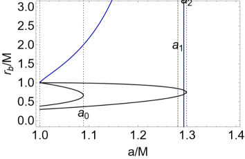
Figure 29: Analysis of inversion plane $\sigma_{\mbox{\scriptsize{{T}}}}$ with fluid specific angular momentum $\ell^{-}$, including co-rotating motion $\ell^{-}>0$ and counter-rotating fluids with $\ell=\ell^{-}<0$ for spin $a\in]M,a_{2}[$ and orbital range for the definition of $\ell$ in $]r_{0}^{-},r_{0}^{+}[-]r_{\delta}^{-},r_{\delta}^{+}[$. Left panel: momentum $\ell^{-}$ on the geodesic radii are shown as function of the NS spin-mass ratios. Reference value $\ell=\ell_{\gamma}^{-}=a$ is shown, function $\ell_{\beta}$ of Eqs. (32) on the geodesic structure (relative to fluid momentum $\ell^{-}$ is also shown. Right panel: Radius $r_{b}$ is plotted on different momenta according to the colors definitions of the right left panel. Spins $\{a_{0},a_{1},a_{2}\}$ are defined in Table (2). Black curves are radii $r_{0}^{-}<r_{\delta}^{-}<r_{\delta}^{+}<r_{0}^{+}$ as functions of the NS spin $a/M$.

Here however we consider also the case $s=+1$. The choice of $s$ sign is related to the sing of $(u^{t},u^{\phi})$ and $(\mathcal{E},\mathcal{L})$. In the following we drop the notation T while still intending all the quantities being evaluated at the inversion point. We consider the normalization condition with $\kappa=\{0,-1\}$ and ($u^{\phi}=0$, $u^{t}>0$), introducing the following quantities

$$\dot{t}_{[u]}\equiv\sqrt{\frac{\Sigma}{\Sigma-2r}};\quad\dot{\theta}^{2}_{[u]}\equiv\frac{r\left[(r-2)\dot{t}^{2}-r\right]-a^{2}(\sigma-1)\left(\dot{t}^{2}-1\right)}{\Sigma^{2}},\quad\dot{\theta}^{2}_{[y]}\equiv\frac{(r-2)\dot{t}^{2}}{r^{3}},\quad\dot{\theta}^{2}_{[g]}\equiv\frac{\dot{t}^{2}\left(\Sigma-2r\right)}{\Sigma^{2}};$$

$$\dot{r}_{[u]}\equiv-\frac{\Delta\left[a^{4}(\sigma-1)^{2}\dot{\theta}^{2}+a^{2}(\sigma-1)\left[\dot{t}^{2}-2r^{2}\dot{\theta}^{2}-1\right]+r^{4}\dot{\theta}^{2}+r^{2}-(r-2)r\dot{t}^{2}\right]}{\Sigma^{2}};$$ (34)

$$\dot{r}^{2}_{[x]}\equiv-\frac{\Delta\left[a^{4}(\sigma-1)^{2}\dot{\theta}^{2}+a^{2}(\sigma-1)\left[\dot{t}^{2}-2r^{2}\dot{\theta}^{2}\right]+r^{4}\dot{\theta}^{2}-(r-2)r\dot{t}^{2}\right]}{\Sigma^{2}}.$$

For photon-like particles there is $\dot{r}^{2}=\dot{r}^{2}_{[x]},\mathcal{L}=\mathcal{L}_{[g]},\mathcal{E}=\mathcal{E}_{[g]}$ with

$$s<0,(\sigma=\sigma_{\epsilon}^{+},r=r_{\epsilon}^{-},\dot{\theta}^{2}=0),(\sigma\in]\sigma_{\epsilon}^{+},1[,(r=r_{\epsilon}^{\pm},\dot{\theta}^{2}=0),(\sigma=1,r=2,\dot{\theta}^{2}=0);$$ (35)

$$s\geq 0:(\sigma\in[0,\sigma_{\epsilon}^{+}[,\dot{\theta}^{2}\in[0,\dot{\theta}^{2}_{[g]}]),(\sigma=\sigma_{\epsilon}^{+},(r\in]0,r_{\epsilon}^{-}[\cup r>r_{\epsilon}^{-},\dot{\theta}^{2}\in[0,\dot{\theta}^{2}_{[g]}]),(r=r_{\epsilon}^{-},\dot{\theta}^{2}=0);$$

$$(\sigma\in]\sigma_{\epsilon}^{+},1[,(r\in]0,r_{\epsilon}^{-}[\cup r>r_{\epsilon}^{+},\dot{\theta}^{2}\in[0,\dot{\theta}^{2}_{[g]}]),(r=r_{\epsilon}^{\pm},\dot{\theta}^{2}=0);$$

$$(\sigma=1,(r=2,\dot{\theta}^{2}=0);(r>2,\dot{\theta}^{2}\in[0,\dot{\theta}^{2}_{[y]}])).$$ (36)

For time-like particles there is $\dot{r}^{2}=\dot{r}_{[u]},\mathcal{L}=\mathcal{L}_{[g]},\mathcal{E}=\mathcal{E}_{[g]}$ with

$$s\geq 0:$$

$$(\sigma\in[0,\sigma_{\epsilon}^{+}[,(\dot{t}=\dot{t}_{[u]},\dot{\theta}^{2}=0);$$

$$(\dot{t}>\dot{t}_{[u]},\dot{\theta}^{2}\in[0,\dot{\theta}^{2}_{[u]}]);$$ (37)

$$(\sigma=\sigma_{\epsilon}^{+},(r\neq r_{\epsilon}^{-},(\dot{t}=\dot{t}_{[u]},\dot{\theta}^{2}=0);$$

$$(\dot{t}>\dot{t}_{[u]},\dot{\theta}^{2}\in[0,\dot{\theta}^{2}_{[u]}]);$$

$$\sigma\in]\sigma_{\epsilon}^{+},1],((r\in]0,r_{\epsilon}^{-}[\cup r>r_{\epsilon}^{+},$$

$$(\dot{t}=\dot{t}_{[u]},\dot{\theta}^{2}=0);(\dot{t}>\dot{t}_{[u]},\dot{\theta}^{2}\in[0,\dot{\theta}^{2}_{[u]}]).$$ (38)

The flow inversion points at $s=+1$ and $s=-1$ are in separated orbital regions and therefore distinguishable. Considering also the normalization condition, with $u^{\phi}=u^{r}=u^{\theta}=0$ (stand still condition), there is $(\mathcal{E}\geq 0,\mathcal{L}\leq 0,\ell\leq 0,u^{\phi}=0)$ with $(\mathcal{E}_{(x)},\mathcal{L}_{(x)},\ell_{(x)}=\mathcal{L}_{(x)}/\mathcal{E}_{(x)},u_{(x)}^{t})$ for: $(s<0,k<0,a>1):(\sigma\in]0,\sigma_{\epsilon}^{+}[,r>0),(\sigma=\sigma_{\epsilon}^{+},r\neq r_{\epsilon}^{-}),(\sigma\in]\sigma_{\epsilon}^{+},1],(r\in]0,r_{\epsilon}^{-}[\cup r>r_{\epsilon}^{+})$. There is $(s>0,k>0,a>1):\sigma\in]\sigma_{\epsilon}^{+},1],r\in]r_{\epsilon}^{-},r_{\epsilon}^{+}[$. Where $u_{(x)}^{t}\equiv\sqrt{k\left({2r}/({2r-\Sigma})-1\right)},\mathcal{E}_{(x)}={ks}/u^{t}$, $\mathcal{L}_{(x)}\equiv-2ar\sigma u^{t}/\Sigma$. The case $\ell=0$ is possible only for $\mathcal{L}=0$ and $\sigma=0$ (on the BH axis) where $\mathcal{E}={u^{t}\Delta}/({a^{2}+r^{2}})$ Considering also the normalization and the stand still condition, the case $\ell=0$ is possible for any $s$ and $\kappa$ only for $\mathcal{L}=0$ and $\sigma=0$ (on the rotational axis), where $\mathcal{E}={\kappa s}/u^{t}$, $u^{t}=\sqrt{-\kappa(a^{2}+r_{\mbox{\scriptsize{{T}}}}^{2})/\Delta_{\mbox{\scriptsize{{T}}}}}$.

Let us define :

$$\mathcal{E}_{\Gamma}\equiv\dot{t_{{\mbox{\scriptsize{{T}}}}}}\left[1-\frac{2r_{{\mbox{\scriptsize{{T}}}}}}{\Sigma_{{\mbox{\scriptsize{{T}}}}}}\right],\quad\mathcal{L}_{\Gamma}=-\frac{2ar_{{\mbox{\scriptsize{{T}}}}}\sigma_{{\mbox{\scriptsize{{T}}}}}\dot{t}_{{\mbox{\scriptsize{{T}}}}}}{\Sigma_{{\mbox{\scriptsize{{T}}}}}},$$ (39)

For $s=-1$ there are no inversion for points for time-like or photon-like particles with $(\mathcal{L}<0,\mathcal{E}<0)$. There are however spacelike solutions (at $u^{t}>0$), in the ergoregion with $(\dot{r}_{{\mbox{\scriptsize{{T}}}}}^{2}=\dot{r}_{J}^{2},\mathcal{L}=\mathcal{L}_{\Gamma},\mathcal{E}=\mathcal{E}_{\Gamma})$ for

$$\sigma_{{\mbox{\scriptsize{{T}}}}}\in]\sigma_{\epsilon}^{+},1],r_{{\mbox{\scriptsize{{T}}}}}\in]r_{\epsilon}^{-},r_{\epsilon}^{+}[,(\dot{t}_{{\mbox{\scriptsize{{T}}}}}\in]0,\dot{t}_{\Gamma}^{-}[,\dot{\theta}_{{\mbox{\scriptsize{{T}}}}}^{2}\in[0,\dot{\theta}^{2}_{J}]);(\dot{t}_{{\mbox{\scriptsize{{T}}}}}=\dot{t}_{\Gamma}^{-},\dot{\theta}^{2}=0),$$ (40)

where

$$\dot{t}_{\Gamma}^{-}\equiv\sqrt{\frac{2r_{{\mbox{\scriptsize{{T}}}}}}{2r_{{\mbox{\scriptsize{{T}}}}}-\Sigma_{{\mbox{\scriptsize{{T}}}}}^{2}}-1};\quad\dot{\theta}^{2}_{J}\equiv\frac{r_{{\mbox{\scriptsize{{T}}}}}\left[(r_{{\mbox{\scriptsize{{T}}}}}-2)\dot{t}_{{\mbox{\scriptsize{{T}}}}}^{2}+r_{{\mbox{\scriptsize{{T}}}}}\right]-a^{2}(\sigma_{{\mbox{\scriptsize{{T}}}}}-1)\left(\dot{t}_{{\mbox{\scriptsize{{T}}}}}^{2}+1\right)}{\Sigma_{{\mbox{\scriptsize{{T}}}}}^{2}};$$ (41)

$$\dot{r}_{J}^{2}\equiv-\frac{\Delta_{{\mbox{\scriptsize{{T}}}}}\left[a^{4}(\sigma_{{\mbox{\scriptsize{{T}}}}}-1)^{2}\dot{\theta}_{{\mbox{\scriptsize{{T}}}}}^{2}+a^{2}(\sigma_{{\mbox{\scriptsize{{T}}}}}-1)\left(\dot{t}_{{\mbox{\scriptsize{{T}}}}}^{2}+1-2r_{{\mbox{\scriptsize{{T}}}}}^{2}\dot{\theta}_{{\mbox{\scriptsize{{T}}}}}^{2}\right)+r_{{\mbox{\scriptsize{{T}}}}}^{4}\dot{\theta}_{{\mbox{\scriptsize{{T}}}}}^{2}-r_{{\mbox{\scriptsize{{T}}}}}\left[(r_{{\mbox{\scriptsize{{T}}}}}-2)\dot{t}_{{\mbox{\scriptsize{{T}}}}}^{2}+r_{{\mbox{\scriptsize{{T}}}}}\right]\right]}{\Sigma_{{\mbox{\scriptsize{{T}}}}}^{2}}.$$

References

- [1] Z. Stuchlik, J. Schee, CQGra, 29, 065002, (2012).
- [2] Z. Stuchlik, J. Schee, CQGra, 27, 215017 (2010).
- [3] R. Shaikh, P. S. Joshi, JCAP, 10, 064 (2019).
- [4] A. B. Joshi, D. Dey, P. S. Joshi, et al.,Phys. Rev. D, 102, 024022, (2020).
- [5] Z. Stuchlik, S. Hledik,& K. Truparova, Class. Quant. Grav., 28, 155017 (2011).
- [6] R. Shaikh, P. S. Joshi, JCAP, 10, 064, (2019).
- [7] P. Bambhaniya, A. B. Joshi, D. Dey, et al. Phys. Rev. D, 100, 124020, (2019).
- [8] M.Rizwan, M. Jamil, and K. Jusufi, Phys. Rev. D, 99, 024050, (2019).
- [9] C. Chakraborty, P. Kocherlakota, M. Patil, et al. Phys. Rev. D, 95, 084024, (2017).
- [10] Jun-Qi Guo et al., CQGra, 38, 035012, (2021).
- [11] Z. Stuchlik, BAICz, 31, 129 (1980).
- [12] Z. Stuchlik, BAICz, 32, 68 (1981).
- [13] P. S Joshi et al., CQGra, 31, 015002, (2014).
- [14] Z. Kovacs, T. Harko, Phys. Rev. D, 82, 124047, (2010).
- [15] D. Pugliese, Z. Stuchlik,MNRAS, 512, 4, 5895–5926. (2022).
- [16] M. Jaroszynski, M. A. Abramowicz, B. Paczynski, Acta Astronm., 30, 1, (1980).
- [17] B. Paczyński, Acta Astron., 30, 4, (1980).
- [18] M. Kozłowski, M. Jaroszyński, M. A. Abramowicz Astron. Astrophys., 63, 209 (1998).
- [19] M. A. Abramowicz& P.C. Fragile, Living Rev. Relativity, 16, 1, (2013).
- [20] R. Shafee, J. C McKinney,R. Narayan, et al.Astrophys. J. , 687, L25, (2008).
- [21] P. C. Fragile, O. M. Blaes, P. Anninois, et al. ApJ, 668, 417-429, (2007).
- [22] J-P. De Villiers,& J. F. Hawley, ApJ, 577, 866 (2002).
- [23] Z. Stuchlík, P. Slaný, & J. Kovar, Class. Quantum Gravity, 26, 215013 (2009)
- [24] O. Porth, et al.arXiv:1611.09720 [GRqc] (2016).
- [25] J. A. Font& F. Daigne, ApJ, 581, L23–L26, (2002).
- [26] D. Pugliese, G. Montani, Phys. Rev. D, 91, 8, 083011, (2015).
- [27] J. F. Hawley, Astrophys. J. , 356, 580 (1990).
- [28] J. F. Hawley, MNRAS, 225, 677, (1987).
- [29] J. F. Hawley, Astrophys. J. , 381, 496 (1991)
- [30] J. F. Hawley, L. L. Smarr, J. R. Wilson, Astrophys. J. , 277, 296 (1984).
- [31] J. A. Font, Living Rev. Relat., 6, 4, (2003).
- [32] Q. Lei, M. A. Abramowicz, P. C. Fragile, et al. A&A., 498, 471, (2008).
- [33] M. A. Abramowicz, Nature, 294, 235– 236, (1981).
- [34] O. M. Blaes, MNRAS, 227, 975-992, (1987).
- [35] O. M. Blaes, MNRAS, 227, 975, (1987).
- [36] D. M. Capellupo, G. Wafflard-Fernandez,& D. Haggard, Astrophys. J. , 836, 1, L8 (2017).
- [37] J. E. McClintock, R. Shafee, R. Narayan, et al.,Astrophys. J. , 652, 518 (2006).
- [38] R. A. Daly, Astrophys. J. , 691, L72 (2009).
- [39] J.H. Krolik&J.F. Hawley, Astrophys. J. , 573, 754 (2002).
- [40] B. C. Bromley, W. A. Miller& V. I. Pariev, Nature (London), 391, 54, 756 (1998).
- [41] M.A. Abramowicz, M. Jaroszynski, S. Kato, et al., A&A, 521, A15 (2010).
- [42] E. Agol & J. Krolik, Astrophys. J. , 528, 161 (2000).
- [43] B. Paczyński, astro-ph/0004129 (2000).
- [44] D. Pugliese&Z. Stuchlik 2022, submitted.
- [45] D. Pugliese&Z. Stuchlík, Astrophys. J.s, 221, 2, 25, (2015).
- [46] D. Pugliese & Z. Stuchlík, CQGra, 35, 10, 105005, (2018).
- [47] D. Pugliese&Z. Stuchlik, CQGra, 38, 14, 145014, (2021).
- [48] D. Pugliese, Z. Stuchlik, PASJ, 73, 5, 1333–1366, (2021).
- [49] D. Pugliese & Z. Stuchlik, JHEAp, 17, 1, (2018).
- [50] D. Pugliese&Z.Stuchlík, Astrophys. J.s, 223, 2, 27, (2016).
- [51] D. Pugliese&Z. Stuchlik, Eur. Phys. J. C 79 4, 288, (2019).
- [52] D. Pugliese & Z. Stuchlík, Astrophys. J.s, 229, 2, 40, (2017).
- [53] D. Pugliese & Z. Stuchlík,Class. Quant. Grav. 35, 18, 185008 (2018)
- [54] D. Pugliese&Z. Stuchlik, PASJ,73, 6, 1497-1539, (2021).
- [55] J. Kovář, P. Slaný, C. Cremaschini, et al., Phys. Rev. D, 90, 044029 (2014).
- [56] Z. Stuchlík, Kološ M., Kovář J., Slaný et al., Univ, 6, 26 (2020).
- [57] Z. Stuchlik, BAICz, 34, 129 (1983).
- [58] Z. Stuchlík & S. Hledík, Physical Review D, 60, 044006 (1999).
- [59] E. G. Gimon, P. Horava, Phys. Lett. B, 672, 299–302, (2009).
- [60] D. Pugliese & G. Montani, Gen. Rel. Grav., 53, 5,51 (2021).