Solving the Regge-Wheeler and Teukolsky equations:
supervised vs. unsupervised physics-informed neural networks

Abstract

Expanding on the research on physics-informed neural networks (PINNs) to solve the eigenvalue problems in black hole (BH) perturbation theory [1], the supervised learning approach was investigated to solve the Regge-Wheeler and Teukolsky equations governing gravitational perturbations of Schwarzschild and Kerr BHs. Previous works have applied unsupervised PINNs to compute quasinormal mode frequencies, i.e. the discrete spectra of eigenvalues that satisfy the BH perturbation equations; however, that was limited to only the zeroth and first overtone (i.e. $n=0,1$). In this paper, supervised learning is used to compute higher overtones with approximation errors accentuated primarily by the input data rather than the PINNs themselves. Our results show the ability of PINNs to approximate overtones up to the limits set by the input data, which concurs with the universal approximation theory of neural networks.

I Introduction

One of the most intriguing aspects of Einstein’s theory of general relativity (GR) is the presence of black holes (BHs) [2, 3, 4], and since the early 20th century when GR first emerged, their characteristics have been thoroughly investigated. The response of BHs to perturbations is of significant interest to both mathematicians and physicists, with a long history in GR [5]. The idea of quasinormal modes (QNMs) is central to this [6, 7, 8], they being oscillations with purely ingoing wave boundary conditions at the BH horizon and purely outgoing wave boundary conditions at far distances.

Recently, QNMs have received renewed interest in light of the detection of gravitational waves, where during the merger of two compact objects, the resulting gravitational wave signal can be roughly split into three distinct parts: The first phase is the inspiral phase, which occurs as the objects attract each other. The second is the catastrophic merger, in which the two objects unify and the majority of the gravitational wave energy is released. The third phase, also known as the ringdown stage, is characterized by the generation of QNMs, during which the final object returns to an equilibrium state [7, 9]. A Kerr BH as the final object requires only two parameters for a complete characterization: its mass and spin. The QNM frequencies have a close connection to these fundamental properties of the Kerr BH, and as such they serve as a distinctive identifier for each BH.

Since Vishveshwara’s work in 1970 [10], the exploration of QNMs in space-times containing BHs has been extensively studied. During his early numerical calculations, he was the first to observe the quasinormal ringing phenomenon in the context of a Schwarzschild BH [10]. This was expanded to include Kerr BHs, which are uncharged rotating BHs in asymptotically flat spacetime, as studied by Teukolsky [11]. The Teukolsky equations being the separable second-order partial differential equations which allow us to calculate the Kerr BH’s QNMs [12, 13].

A wide range of methods for solving these equations has been developed, including Leaver’s approach (also known as the continued fraction method (CFM)), which has become a recognized standard for finding QNM frequencies in cases including the Schwarzschild and Kerr BHs [13]. In the Kerr BH scenario, Leaver’s method starts with the Teukolsky equations consisting of radial and angular parts, where a Frobenius series is used as an ansatz. This procedure produces recursion relations, which are then transformed into two sets of infinite continued fraction equations. These equations require the determination of a set of minimal solution sequences that correspond to the complex QNM frequencies $\omega_{n}$ and the separation constants $A_{\ell m}$ (related to the separation of the radial and angular equations). Both of these eigenvalues must be calculated numerically. This entire procedure is carried out while the BH spin parameter $a$ remains constant, which falls within the range $0\leq a<0.5$ given we are using the units $c=G=2M=1$. Various modifications to this method have been proposed over the years [14] and a Python package called qnm, which is based on this method, was introduced in Ref. [15]. These and other numerical and semi-analytical approaches have all had limitations, limiting the accuracy and range of QNMs calculated, as discussed in Refs. [16, 17].

In looking to new, and more robust numerical methods, we shall here explore deep learning approaches. Note that deep learning has seen notable success in a variety of applications [18], though its application to differential equations is a relatively recent development that has given rise to a new sub-field known as Scientific Machine Learning (SciML) [19, 20]. Physics-informed neural networks (PINNs), neural networks utilized to solve differential equations, were put forth in Ref. [20], where the algorithm was used to solve forward and inverse problems occurring in common physical scenarios. The method is mesh-free, which eliminates the discretization errors inherent in standard numerical techniques that require mesh generation. The fundamental innovation of this approach is how it reframes the problem from one of directly solving governing equations to one of optimization where the goal is to minimize a loss function. It consists of terms that represent the differential equation “residual” (i.e. the mean of the differential equation squared) at particular domain points (referred to as collocation points), as well as the initial and boundary conditions.

In this paper, the equations governing the gravitational perturbations of Schwarzschild and Kerr BHs are solved using supervised PINNs, wherein the neural networks (NNs) are fed labeled data to enforce constraints that fix the QNM overtone. We then perform a comparative analysis with results from the CFM to assess the robustness of our findings. As such, this paper is structured as follows: In section II we present BH perturbation theory as concerned with the propagation of fields in the curved space-times of the Schwarzschild and Kerr BHs. Subsequently, section III elaborates on unsupervised and supervised learning in the context of PINNs. Finally, section IV gives the results of our QNM calculations and we conclude in section V.

II Black hole perturbation theory: asymptotically flat space-times

II.1 Schwarzschild black hole

To obtain the equations governing the propagation of fields of various spins within a BH metric, we consider their respective equations of motion in asymptotically flat space-times that impose astrophysical boundary conditions on the QNMs, such that the only physically allowed wavefunctions are at the BH event horizon and outgoing at spatial infinity, with an exponential decay in the temporal domain. When considering the Schwarzschild BH, this asymptotic behavior of QNMs $\psi(x)$ is expressed as:

$$\lim_{x\to-\infty}=e^{-i\omega x};\quad\lim_{x\to\infty}=e^{i\omega x}.$$ (1)

Note that $x$ is a tortoise coordinate associated with the radial coordinate $r$ according to:

$$x(r)\ =\ r+2M\ln{\left(-2M\ +\ r\right)},$$ (2)

for a Schwarzschild BH with one event horizon. Note that the boundary conditions and the tortoise coordinate differ in form from Eqs. (1) and (2) when considering the Kerr metric, which we explicitly discuss in section II.2.

The derivation of the equation governing the “first-order changes away from the Schwarzschild metric” (the gravitational field perturbations of a Schwarzschild BH) was done in Ref. [21]. Essentially, we consider a perturbating quantity $h_{\mu\nu}$ that is very small compared to the BH metric (i.e. $h_{\mu\nu}\ll g^{0}_{\mu\nu}$) such that the metric tensor of a linearly perturbed metric is given as:

$$g_{\mu\nu}=g^{0}_{\mu\nu}+h_{\mu\nu},$$ (3)

where $g^{0}_{\mu\nu}$ denotes the unperturbed metric:

$$ds^{2}=g^{0}_{\mu\nu}dx^{\mu}dx^{\nu}=-f(r)dt^{2}+f(r)^{-1}dr^{2}+r^{2}d\theta^{2}+r^{2}\sin^{2}{\theta}d\phi^{2}.$$ (4)

This is in Schwarzschild coordinates and we have $f(r)=1-2M/r$, which is the Schwarzschild metric function, and $M$ is the BH mass.

The equations for the gravitational perturbations of a Schwarzschild BH emerge out of the vacuum Einstein equations with $g_{\mu\nu}$ given by Eq. (3) with a perturbation quantity $h_{\mu\nu}$. As shown in Ref. [11], odd and even parity perturbations (axial and polar perturbations, respectively) are obtained from generalizing the spherical harmonic development of scalar quantities to tensor quantities. Through this development, a system of second-order ordinary differential equations (ODEs) is obtained that can be reduced to a single differential equation (the Regge-Wheeler equation when we have axial perturbations):

$$\frac{\partial^{2}Q}{\partial x}+[\omega^{2}-V(r)]Q=0,$$ (5)

with

$$V(r)=\begin{cases}f(r)\left[\dfrac{\ell(\ell+1)}{r^{2}}-\dfrac{6M}{r^{3}}\right],\quad\text{odd parity,}\\ \\ \dfrac{2f(r)}{r^{3}}\times\dfrac{9M^{3}+3c^{2}Mr^{2}+c^{2}(1+c)r^{3}+3M^{2}(3cr+3r^{3}/R^{2})}{(3M+cr)^{2}},\quad\text{even parity.}\end{cases}$$ (6)

Here Q denotes the odd parity wave function whose associated QNMs are identical to those of the even parity wave function due to isospectrality [9]; therefore, it is sufficient to only compute the QNMs from Eq. (5) for the odd parity effective potential.

II.2 Kerr black hole

For gravitational perturbations of a Kerr metric, as was done for the Schwarzschild BH, we consider changes to the metric tensor (Eq. (3)) and the associated Einstein field equations expanded to first order in $h_{\mu\nu}$. The derivation is given in Ref. [11] using the Newman-Penrose formalism, which enables a separability of variables to be achieved in the perturbation equations despite the absence of spherical symmetry.

The separated, source-free (vacuum) equations for perturbations of a Kerr BH by fields of “spin weight” $s$ are obtained from considering the fields separated in spherical co-ordinates according to [11]:

$$\psi=e^{-i\omega t}e^{im\phi}S(\theta)R(r).$$ (7)

For gravitational fields (with $s=-2$) the field is $\psi=\rho^{-4}\psi_{4}$, where $\rho=-1/(r-ia\cos{\theta})$, $a$ is the BH spin and $\psi_{4}$ is a Weyl scalar that is given by $\psi_{4}=\ddot{h}_{+}+i\ddot{h}_{x}$, where $h_{+}$ and $h_{x}$ are the “plus” and “cross” polarisations of gravitational radiation, both observable physical quantities. The separated perturbation equations, known as the Teukolsky equations, are [11, 13]:

$$\Delta^{-s}\dfrac{d}{dr}\left(\Delta^{s+1}\dfrac{R}{r}\right)+\left(\dfrac{K^{2}-2is(r-M)K}{\Delta}+4is\omega r-\lambda\right)R=0,\\$$ (8)

$$\dfrac{d}{du}\left[(1-u^{2})S\right]+\left[a^{2}\omega^{2}u^{2}-2a\omega su+s+A-\dfrac{(m+su)^{2}}{1-u^{2}}\right]S=0,$$ (9)

with $K=(r^{2}+a^{2})\omega-am$, $\lambda=A+a^{2}\omega^{2}-2am\omega$, $\Delta=r^{2}-r+a^{2}=(r-r_{+})(r-r_{-})$, $r_{\pm}=(1\pm\sqrt{1-4a^{2}})/2$ and $u=\cos{\theta}$. Imposing regularity at $\theta=0$ and $\theta=\pi$ on the angular ODE (Eq. (9)) yields an eigenvalue problem, with the separation constant $A=A_{\ell m}$ as eigenvalues and the spheroidal harmonics $S$ as eigenfunctions. In the Schwarzschild limit ($a=0$) the separation constant reduces to:

$$\lim_{a\rightarrow 0}A_{\ell m}=\ell(\ell+1)-s(s+1).$$ (10)

For the radial equation (Eq. (8)), the relevant boundary conditions (imposing ingoing sinusoids at the outer horizon of the Kerr BH and outgoing sinusoids at spatial infinity) are expressed as [22]:

$$\lim_{x\rightarrow-\infty}R=\dfrac{e^{ikx}}{\Delta^{s}},\lim_{x\rightarrow\infty}R=\dfrac{i\omega x}{r^{2s+1}},$$ (11)

where $k=\omega-m\Omega_{H}$, with $\Omega_{H}$ as the angular frequency of the outer horizon $\Omega_{H}=a/(2Mr_{+})$. Here the tortoise coordinate $x$ is given by $dx=(r^{2}+a^{2})/\Delta dr$ or:

$$x=r+\dfrac{r^{2}_{+}+a^{2}}{r_{+}-r_{-}}\ln{\left(\dfrac{r-r_{+}}{r_{+}}\right)}-\dfrac{r^{2}_{-}+a^{2}}{r_{+}-r_{-}}\ln{\left(\dfrac{r-r_{-}}{r_{+}}\right)}.$$ (12)

In solving the Teukolsky equation using the CFM, Ref. [13] utilized an ansatz of $R(r)$ that satisfies the boundary conditions and is given as:

$$R(r)=e^{i\omega r}(r-r_{-})^{-1-s+i\omega+i\sigma_{+}}(r-r_{+})^{-s-i\sigma_{+}}\times f(r).$$ (13)

Here $\sigma_{+}=(\omega r_{+}-am)/\sqrt{1-4a^{2}}$. For the angular differential equation, the required regularity at $\theta=0$ and $\theta=\pi$ is imposed by:

$$S(u)=e^{a\omega u}(1+u)^{|m-s|/2}(1-u)^{|m+s|/2}\times g(u).$$ (14)

With Eqs. (13) and (14), the radial and angular differential equations can be given in terms of $f(x)$ and $g(u)$, respectively, ensuring the required asymptotic behavior is incorporated in the equations. When applying PINNs to solve the Teukolsky equation, the radial and angular ODEs in terms of $f(x)$ and $g(u)$ are incorporated within the loss function such that $f(x)$ and $g(u)$ are approximated by the NNs. This follows the same procedure used in Ref. [23].

III Physics-informed neural networks

PINNs utilize the mechanism underlying standard NNs that involves the same elements as a regression problem: a “trial function” with tunable parameters, an error function (or loss function using the language of NNs), and a dataset to fit the model. While the analogs of a trial function and error exist in PINNs, in general, they do not require a dataset for constraining the NN model [19]. More broadly speaking, physical constraints can be imposed directly onto PINNs by incorporating the differential equations in the loss function as opposed to providing them empirically through a training dataset. With the differential equation in the loss function as an NN regularizer, the approximate solution of the given differential equation, denoted by $\hat{f}(x)$, is generated by the NN output through the minimization of the loss function using the same optimization algorithm as is done within standard deep learning [20]. For the specific case of eigenvalue problems, the differential equations to be solved generally take the form:

$$\mathcal{L}f(x)=\lambda f(x),$$ (15)

where $\mathcal{L}$ is a differential operator that depends on a spatial variable $x$, while $f(x)$ and $\lambda$ denote eigenfunction and eigenvalue, respectively. The output of PINNs is a composite function constructed from matrix operations that are linear transformations acting on layers of parameter vectors, expressed by the recurrence relation:

$$\quad\mathcal{N}^{\ell}(\mathbf{x})=\sigma\left(\mathcal{N}^{\ell-1}(\mathbf{x})\mathbf{W}^{\ell}+\mathbf{b}^{\ell}\right),\quad\text{for}\quad 1\leq\ell\leq L.$$ (16)

The output layer $\mathcal{N}^{\ell=L}(\mathbf{x})$ is used to represent the eigenfunction $f(x)$ in Eq. (15). In general, for each NN layer $\ell$, $\mathcal{N}^{\ell}(\mathbf{x})$ is the output vector which is the outcome from multiplying an “input” vector (the previous layer) $\mathcal{N}^{\ell-1}(\mathbf{x})$ with a matrix of weights $\mathbf{W}^{\ell}$ and adding a bias matrix $\mathbf{b}^{\ell}$ (see Eq. (16)). The quantities $\mathbf{W}^{\ell}$ and $\mathbf{b}^{\ell}$ signify tunable parameters whose values are arbitrarily initialized before the NN is trained and are updated in the course of training when the approximated $\hat{f}(x)$ is tuned towards the target solution $f(x)$. Furthermore, $\sigma$ in Eq. (16) represents a non-linear activation function applied to each hidden layer of the NN (excluding the output layer) facilitating the approximation of a broad family of differentiable functions, as per the universal approximation theory of NNs [24, 19].

The PINN algorithm entails several iterations of forward- and backward-passes through the network. The randomly initialized weight and bias matrices have elements selected from probability distributions, such as the uniform distribution: $\mathcal{U}(-\sqrt{k},\sqrt{k})$, where $k=1/N$ and $N$ is the number of input layer neurons. Each cycle of forward- and backward-passes propagates input data through the NN and backpropagates the derivatives of the loss function which are used to update the NN weight and bias matrices in each optimization step. For example, with the stochastic gradient descent (SGD) algorithm, a standard optimization algorithm, each update carries out the following transformations:

$$w^{\ell} \rightarrow w^{\ell}-\frac{\eta}{m}\sum_{x}\frac{\partial\mathcal{L}_{x}}{\partial w^{\ell}},$$ (17)

$$b^{\ell} \rightarrow b^{\ell}-\frac{\eta}{m}\sum_{x}\frac{\partial\mathcal{L}_{x}}{\partial b^{\ell}},$$ (18)

where $w^{\ell}$ and $b^{\ell}$ signify each of the weight and bias elements in a given NN layer $\ell$ and the summations are over all the $m$ input data points that constitute a minibatch of a dataset utilized in one given forward-backward pass and subsequent update step. The term $\eta$ is a small, positive parameter, the learning rate, that determines how quickly the weights and biases are updated. A variation of the SGD that is often the standard optimization algorithm is the adaptive moment estimation (Adam) optimizer proposed by Ref. [25].

A crucial feature that enables the implementation of the mentioned algorithms and the relevant equation is automatic differentiation. With this tool, it is possible to compute the exact numerical values of the derivatives used within backpropagation and the optimization algorithm (Eqs. (17) and (18)). This capability to numerically compute derivatives is taken advantage of in PINN when we incorporate ODEs, such as Eq. (15), into the loss function without the need for discretization, as is carried out with traditional numerical methods.

III.1 Unsupervised physics-informed neural networks

The idea of using unsupervised (data-free) PINNs to solve eigenvalue problems was adopted from the paper by Jin, Mattheakis, and Protopapas [26] who used the approach to solve quantum Sturm-Liouville differential equations involving the 1D time-independent Schrödinger equation. In our previous work [1], we adopted this approach to solve the radial equation governing perturbations of a Schwarzschild BH whose form resembles the 1D Schrödinger equation insofar as being a second-order linear differential equation and an eigenvalue problem; however, the difference lies in that the former is non-Hermitian and has a spectrum of complex-valued eigenvalues.

Unsupervised NNs differ from the standard supervised setup in terms of how the physics constraints are imposed on the NN model. In the former, we impose differential equations and associated boundary conditions as constraints, while in the latter, the constraints are in the form of a labeled dataset that implicitly captures the physical laws. In both scenarios, the constraints are subsumed in the loss function to incorporate the physics knowledge in the NN optimization. Both constraints can be included in the loss simultaneously or used separately. The most general approach to using PINNs to solve eigenvalue problems, as far as we know, is the unsupervised method where it is sufficient to only know the governing equations and the relevant boundary conditions.

In our implementation of this approach in Ref. [1], the solutions we obtained had the same level of numerical precision as the standard approaches, mainly the CFM that was used for comparison [13]. The results were remarkable in terms of computing the fundamental mode frequencies, particularly given the simplicity of implementing PINNs. However, there remained the challenge of learning overtones (distinguished by the overtone number $n$ which is implicit within the definition of the eigenvalue problem). This challenge is also seen in the recent work by Luna et al. [23], who generated the QNMs of Kerr BHs for a small part of the QNM spectrum (i.e. only the fundamental mode and first overtone ($n=1$)) even when “seed values” were used within the loss functions to loosely constrain the NN (in a similar manner to the use of seed values in methods such as the asymptotic iteration method [27]).

In our implementation of this approach in Ref. [1], the solutions we obtained had the same level of numerical precision as the standard approaches, mainly the CFM that was used for comparison [13]. The results were remarkable in terms of computing the fundamental mode frequencies, particularly given the simplicity of implementing PINNs. However, there remained the challenge of learning overtones (distinguished by the overtone number $n$ which is implicit within the definition of the eigenvalue problem). This challenge is also seen in the recent work by Luna et al. [23], who generated the QNMs of Kerr BHs for a small part of the QNM spectrum (i.e. only the fundamental mode and first overtone ($n=1$)) even when “seed values” were used within the loss functions to loosely constrain the NN (in a similar manner to the use of seed values in methods such as the asymptotic iteration method [27]).

In our implementation of this approach in Ref. [1], the solutions we obtained had the same level of numerical precision as the standard approaches, mainly the CFM that was used for comparison [13]. The results were remarkable in terms of computing the fundamental mode frequencies, particularly given the simplicity of implementing PINNs. However, there remained the challenge of learning overtones (distinguished by the overtone number $n$ which is implicit within the definition of the eigenvalue problem). This challenge is also seen in the recent work by Luna et al. [23], who generated the QNMs of Kerr BHs for a small part of the QNM spectrum (i.e. only the fundamental mode and first overtone ($n=1$)) even when “seed values” were used within the loss functions to loosely constrain the NN (in a similar manner to the use of seed values in methods such as the asymptotic iteration method [27]).

In applying the unsupervised approach to generate the QNMs of Kerr BHs we have seen that the accuracy diminishes (compared to results that exist within the literature) with increasing BH spin. To gather insight on the required refinements of the approach needed to facilitate computing accurate QNMs and higher overtones, the supervised approach has been adopted in this paper to compute the gravitational perturbations of Schwarzschild and Kerr BHs.

III.2 Supervised physics-informed neural networks

When a supervised approach is utilized, PINNs solve inverse-type problems and the loss function is given, in general, as [19]:

$$\mathcal{L}(\mathbf{\theta};\mathcal{T})=w_{DE}\mathcal{L}_{DE}(\mathbf{\theta};\mathcal{T})+w_{BC}\mathcal{L}_{BC}(\mathbf{\theta};\mathcal{T})+w_{data}\mathcal{L}_{data}(\mathbf{\theta};\mathcal{T}),$$ (19)

where $w_{DE},w_{BC},w_{data}$ are user-defined weights and while $\mathbf{\theta}=\{\textbf{W}^{\ell},\textbf{b}^{\ell}\}_{1\leq\ell\leq L}$ with $\ell$ specifying a NN layer and $\textbf{W}^{\ell},\textbf{b}^{\ell}$ are as defined in Eq. (16). Training points randomly selected from the computational domain are denoted by $\mathcal{T}$ and the functions $\mathcal{L}_{DE}$ and $\mathcal{L}_{BC}$ are the differential equation residual and boundary condition loss terms, respectively:

$$\mathcal{L}_{DE}(\mathbf{\theta};\mathcal{T}) = \frac{1}{|\mathcal{T}_{DE}|}\sum_{\mathbf{x}\in\mathcal{T}_{DE}}\left\lVert f(\mathbf{x};\frac{\partial\hat{u}}{\partial x_{1}},\ldots,\frac{\partial\hat{u}}{\partial x_{d}};\frac{\partial^{2}\hat{u}}{\partial x_{1}\partial x_{1}},\ldots,\frac{\partial^{2}\hat{u}}{\partial x_{d}\partial x_{d}};\hat{\mathbf{\lambda}})\right\rVert^{2}_{2},$$ (20)

$$\mathcal{L}_{BC}(\mathbf{\theta};\mathcal{T}) = \frac{1}{|\mathcal{T}_{BC}|}\sum_{\mathbf{x}\in\mathcal{T}_{BC}}\left\lVert\mathcal{B}(\hat{u},\mathbf{x})\right\lVert^{2}_{2},$$ (21)

where the “hat” notation of $\hat{u}$ and $\hat{\mathbf{\lambda}}$ signify the NN’s approximations of the response variable $u(\mathbf{x})$ and any unknown coefficients or eigenvalues within differential equations. The loss term $\mathcal{L}_{data}$ represents, for inverse problems, the mean square error of $\hat{u}(\mathbf{x})$ when compared to a “labeled dataset” of the response variable $u(\mathbf{x})$:

$$\mathcal{L}_{data}(\mathbf{\theta};\mathcal{T})=\frac{1}{|\mathcal{T}_{data}|}\sum_{\mathbf{x}\in\mathcal{T}_{data}}\left\lVert u(\mathbf{x})-\hat{u}(\mathbf{x})\right\rVert^{2}_{2}.$$ (22)

As such, inverse problems require a dataset of target values $u(\mathbf{x})$ for optimization. Applying this approach to the Regge-Wheeler and the Teukolsky equations, a natural first step is to generate a dataset of the QNM eigenfunctions using other numerical techniques. In this paper, we utilized the CFM [13] implemented using a Mathematica code.

Datasets consisting of $\sim 10^{3}$ points were generated to act as BH spin and overtone number dependent “seed values” used to train the PINNs. During NN optimization, the eigenvalues of the differential equation are inferred from the associated eigenfunctions represented by the NNs in the typical way that inverse problems are solved. The performance of this approach is limited in part by the approximation errors inherited from the numerical techniques for data generation, in this case, the CFM. Nevertheless, our results (see section IV) indicate that the universal approximation theory of NN holds in approximating the QNMs of BHs: i.e. given sufficiently well-defined physical constraints, NN approximation can converge to the different, physically allowed eigenstates that make up the eigenspectrum of a given eigenvalue problem.

In solving the perturbation equations of interest, we utilize the same notation used by Leaver [13]. Regarding the gravitational perturbations of a Schwarzschild BH, we consider solving:

$$F_{0}f^{\prime\prime}(\xi)+F_{1}f^{\prime}(\xi)+F_{2}f(\xi)=0,$$ (23)

with

$$F_{2} = -(\ell(1+\ell)+\epsilon(\xi-1)-4\rho(\xi-2\rho+\xi\rho-1)),$$ (24)

$$F_{1} = (1+2\rho-4\xi(1+2\rho)+\xi^{2}(3+4\rho)),$$ (25)

$$F_{0} = (\xi-1)^{2}\xi.$$ (26)

Here we have carried out a change in coordinates from $r\in[2M,\infty)$ to $\xi\in[0,1]$ using the transformation $\xi=(r-2M)/r$ (note that we are working in the units: $c=G=2M=1$). This transformation is necessary for obtaining a finite domain that facilitates solving the problem numerically, considering we cannot work with infinity in our numerical setup. As is outlined in Ref. [13], $\epsilon=s^{2}-1$ (where $s$ is the spin-weight of the perturbating field) and $\epsilon=3$ for gravitational fields. The QNM frequency is denoted by $\rho=-i\omega$. The boundary conditions for Schwarzschild BHs (Eq. (1)) are automatically satisfied by Eq. (23) which is derived from imposing an ansatz of the solution given as:

$$\psi=e^{-\xi\rho/\xi-1}(1/1-\xi)^{2\rho}(\xi/1-\xi)^{\rho}f(\xi).$$ (27)

Evaluating Eq. (23) at given points in the computational domain specified by the input data points and taking the mean of the square gives $\mathcal{L}_{DE}$ in this case, while $\mathcal{L}_{data}$ is the mean square error of the PINN approximations $\hat{f}(\xi)$ compared with the associated target values provided by the dataset of points $f(\xi)$ within the domain of $\xi$.

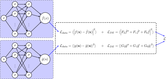
Figure 1: A schematic of the PINN used to approximate the functions $f(x)$ and $g(x)$ and their derivatives such that the governing Eqs. (30) and labelled data are satisfied.

For gravitational perturbations of a Kerr BH, the relevant boundary conditions of the radial and angular equations are given as [13]:

$$R(r) = e^{i\omega r}(r-r_{-})^{-1-s+i\omega+i\sigma_{+}}(r-r_{+})^{-s-i\sigma_{+}}f(x),\quad\sigma_{+}=\frac{\omega r_{+}-am}{\sqrt{1-4a^{2}}},$$ (28)

$$S(u) = e^{a\omega u}(1+u)^{|m-s|/2}(1-u)^{|m+s|/2}g(u),$$ (29)

where $u=\cos{\theta}$, $x=r_{+}/r$ and $r_{\pm}=(1\pm\sqrt{(1-4a^{2})})/2$. In both the radial and angular equations, we are using finite domains; that is, $x\in[0,1]$ and $u\in[-1,1]$, respectively. As was done in Ref. [23], Eqs. (8) and (9) can be given in terms of $f(x)$ and $g(u)$ in the form:

$$F_{2}f^{\prime\prime}+F_{1}f^{\prime}+F_{0}f=0,\quad G_{2}g^{\prime\prime}+G_{1}g^{\prime}+G_{0}g=0,$$ (30)

where the coefficients $F_{i}=F_{0,1,2}$ and $G_{i}=G_{0,1,2}$ are functions of $x$ and $u$, respectively (see Ref. [23] for the full expressions). Solving the Teukolsky equation with PINNs is facilitated by constructing two separate NNs to approximate $f(x)$ and $g(u)$ and, in turn, satisfy the Eqs. (30). The setup is illustrated in Fig. 1, where the mean squares of the differential equations are incorporated into the loss function in addition to the mean square errors that take into account the labeled data. A similar setup applies to the PINNs used for computing the QNMs of a Schwarzschild BH using supervised learning.

Regarding the implementation of PINNs in code, we use the PyTorch library extensively for defining the tensors, linear transformation, activation functions, and automatic differentiation required to create neural network algorithms. The code was run using Jupyter Notebooks on Google Colaboratory (Colab) considering that we did not require a lot of computational memory to create the graphs that constitute PyTorch NNs. The specifics of the Google Colab set-up that we used are the following: Intel(R) Xeon(R) CPU @ 2.20GHz and 12GB of usable RAM.

IV Eigenvalues of the differential equations governing gravitational perturbations of Schwarzschild and Kerr black holes

Given in this section are the QNM eigenvalues computed using supervised PINNs. These results show that, given a grid of labeled data points selected from the computational domain (e.g. the radial and angular domains relevant to the Teukolsky equation), PINNs can simultaneously determine the eigenfunctions that concur with input data and the associated QNM frequencies not known beforehand. We selected a training dataset that had minimal approximation errors such that we could minimize the propagation of those errors in the PINN algorithm. Note that the errors indicated in our results include this pre-existing numerical error from CFM, which is independent of the performance of PINNs. It becomes more significant as the overtone numbers and BH spin (for the Kerr case) increase. As such, the PINN algorithm is demonstrated for that part of the $0\leq a<0.5$ range where we have good constraints and the integrity of the loss function (that is, the interplay between the data and the differential equations) supports the approximation of the desired QNMs.

While varying the physical parameters of the perturbation equations (i.e. overtone number and BH spin), the hyperparameter configurations of the PINNs were fixed. In terms of the hyperparameters associated with the NN structure, 1 hidden layer with 50 neurons was used for the Schwarzschild case, while we had differing numbers of hidden layers for the radial and angular NNs of the Kerr case (i.e. 2 hidden layers for the radial NN and 1 hidden layer for the angular NN, with 20 neurons per layer in both cases). Regarding the optimization set-up, training was run over $10^{4}$ epochs for both BH scenarios, while learning rates of $5\times 10^{-3}$ and $2\times 10^{-3}$ were used specifically for the Kerr and Schwarzschild cases, respectively. These set-ups were selected arbitrarily and are not based on hyperparameter optimization; therefore, maximizing the performance of our computations can still potentially be achieved by systematic hyperparameter tuning.

Furthermore, in each layer, a self-scalable tanh activation function was used [28] because of its tunability during neural network training. It is given as:

$$\sigma^{k}_{\ell}=\tanh{(\mathbf{x})}+\beta^{k}_{\ell}\mathbf{x}\tanh{(\mathbf{x})},$$ (31)

where $k$ and $\ell$ indicate the neuron number and layer number, respectively. The tunable parameter $\beta^{k}_{\ell}$ is akin to the bias parameter within Eq. (16) and is likewise updated during NN optimization.

Table 1: PINN approximations of the gravitational perturbations of a Schwarzschild BH.

		CFM	unsupervised PINN	supervised PINN
$\ell$	$n$	$\omega_{\textsubscript{$n$}}$	$\omega_{\textsubscript{$n$}}$	$\omega_{\textsubscript{$n$}}$
2	0.0	0.747343 - 0.177925i	0.482324 - 0.403939i	0.747275 - 0.177815i
			(-35.46%)(127.0%)	(-0.001%)(-0.062%)
	1.0	0.693422 - 0.547830i	0.717890 - 0.177626i	0.693320 - 0.547713i
			(3.529%)(-67.58%)	(-0.015%)(-0.021%)
	2.0	0.602107 - 0.956554i	0.731018 - 0.169060i	0.602077 - 0.956616i
			(21.41%)(-82.33%)	(-0.005%)(0.007%)
	3.0	0.503010 - 1.410296i	0.751765 - 0.180630i	0.501597 - 1.411399i
			(49.45%)(-87.19%)	(-0.281%)(0.078%)
3	0.0	1.198887 - 0.185406i	1.198786 - 0.185340i	1.198889 - 0.185402i
			(-0.001%)(-0.032%)	(0.000%)(-0.002%)
	1.0	1.165288 - 0.562596i	1.199539 - 0.185089i	1.165288 - 0.562596i
			(2.947%)(-67.10%)	(-0.007%)(0.021%)
	2.0	1.103370 - 0.958186i	1.198802 - 0.185330i	1.103938 - 0.958909i
			(8.646%)(-80.66%)	(0.051%)(0.075%)
	3.0	1.023924 - 1.380674i	1.198949 - 0.185519i	1.026300 - 1.372778i
			(17.08%)(-86.56%)	(0.232%)(-0.572%)

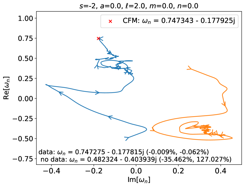
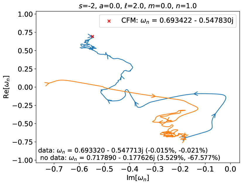
Figure 2: Representation in the complex plane of the evolution of PINN approximations of overtones $\omega_{n\geq 0}$ for the spinless case of a Kerr BH. Shown are QNMs with overtone numbers obtained using supervised learning (blue line) and unsupervised learning (orange line). The arrows indicate the direction of increased learning and are placed at intervals of 100 training epochs.

Table 2: PINN approximations of $\left\{\omega_{n=0,m=0,1},A_{\ell m}\right\}$ and Kerr BH spin $a=0.1,0.2,0.3,0.4$.

		CFM		PINN
$m$	$a$	$\omega_{\textsubscript{$0$}}$	$A_{\textsubscript{$\ell m$}}$	$\omega_{\textsubscript{$0$}}$	$A_{\textsubscript{$\ell m$}}$
0	0.1	0.7502 - 0.1774i	3.9972 + 0.0014i	0.7509 - 0.1762i	3.9989 + 0.0044i
				(0.091%)(-0.651%)	(0.043%)(-0.575%)
	0.2	0.7594 - 0.1757i	3.9886 + 0.0056i	0.7610 - 0.1718i	3.9851 + 0.0020i
				(0.212%)(-2.180%)	(-0.086%)(-0.757%)
	0.3	0.7761 - 0.1720i	3.9730 + 0.0126i	0.7816 - 0.1611i	3.9731 + 0.0016i
				(0.705%)(-6.307%)	(0.003%)(-1.401%)
	0.4	0.8038 - 0.1643i	3.9480 + 0.0223i	0.8177 - 0.1312i	3.9494 + 0.0014i
				(1.719%)(-20.159%)	(0.035%)(-2.041%)
1	0.1	0.7765 - 0.1770i	3.8932 + 0.0252i	0.7770 - 0.1761i	3.8932 + 0.0248i
				(0.059%)(-0.512%)	(0.001%)(-4.879%)
	0.2	0.8160 - 0.1745i	3.7676 + 0.0532i	0.8180 - 0.1714i	3.7668 + 0.0469i
				(0.249%)(-1.812%)	(-0.00%)(-0.605%)
	0.3	0.8719 - 0.1691i	3.6125 + 0.0835i	0.8779 - 0.1609i	3.6110 + 0.0574i
				(0.680%)(-4.887%)	(-0.041%)(-12.999%)
	0.4	0.9605 - 0.1559i	3.4023 + 0.1122i	0.9691 - 0.1303i	3.3899 + 0.0468i
				(0.898%)(-16.406%)	(-0.362%)(-14.296%)

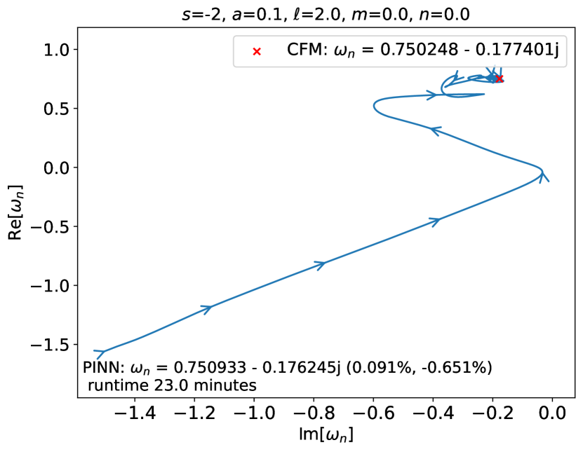
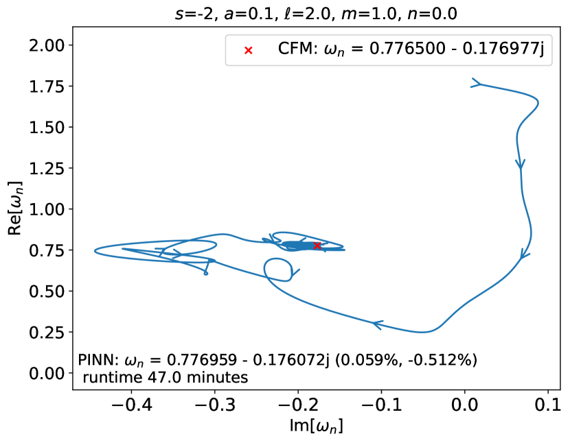
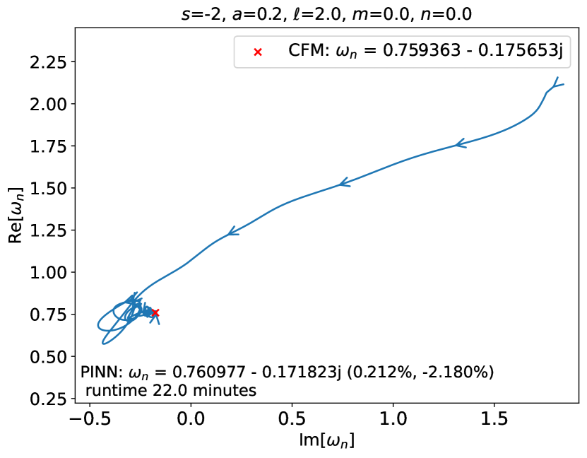
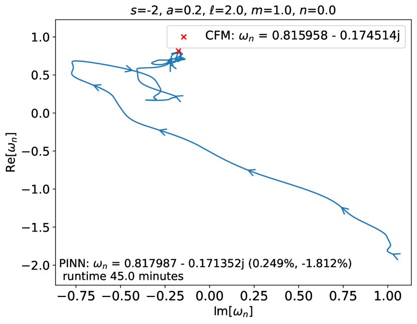
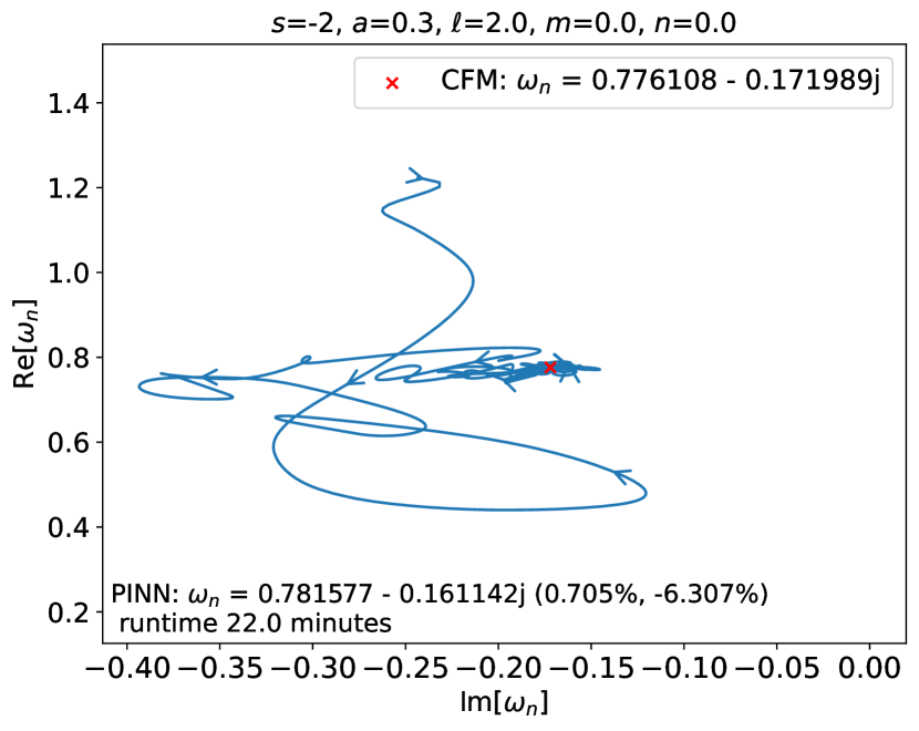
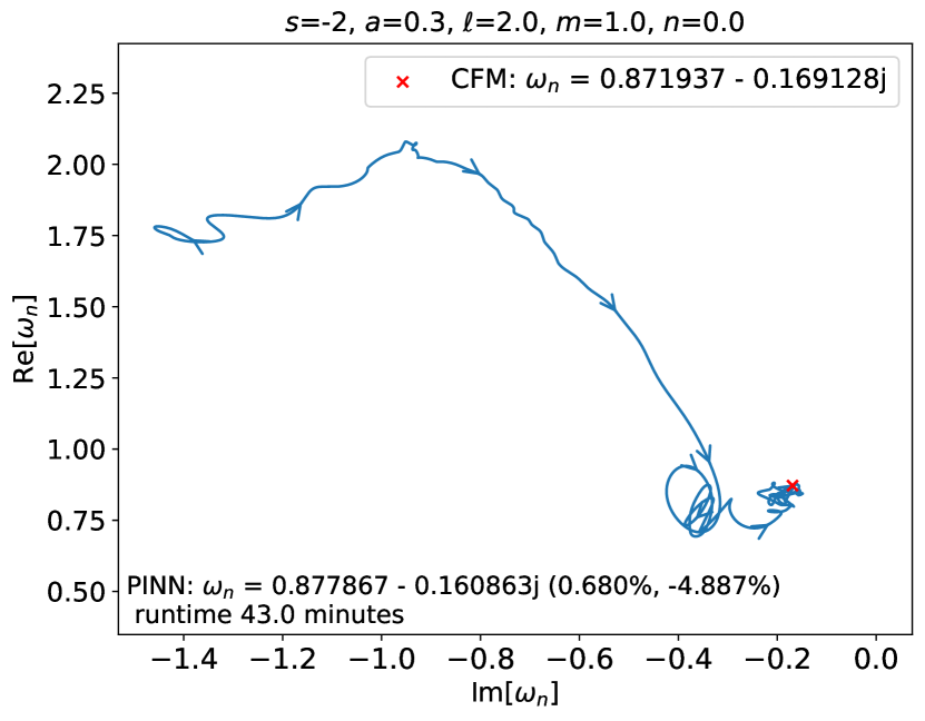
Figure 3: Representation in the complex plane of the evolution of PINN approximations of $\omega_{n=0,m=0,1}$ for the magnitudes of the BH spin $a=0.1,0.2,0.3$ in the course of 10,000 training epochs. The arrows indicate the direction of increased learning and are placed at intervals of 100 training epochs.

Concerning NN optimization, note that the selected learning rates specify the step sizes taken by the Adam optimizer in the course of training. For the Kerr case, where we require two NNs to approximate the radial and angular eigenfunctions, each of the optimization steps takes place after a sequence of linear transformations is executed in both NNs. As such, the learning of the radial and angular eigenfunction using PINNs effectively takes place simultaneously. Each forward and backward pass takes an input vector of $\sim 100$ minibatch points which are used in each NN update step. As many of these update iterations take place in a single training epoch, as there are minibatches in a training dataset to run through. For the sizes of our datasets, we used $\sim 10^{3}$ points for the Schwarzschild case, and in the Kerr case, $\sim 10^{3}$ points for the radial NNs in the Kerr case and $\sim 2\times 10^{3}$ points for the angular NNs. These were points selected from the finite “radial” and angular coordinates: $x\in[0,1]$ and $u\in[-1,1]$, respectively.

Given in Table 1 are QNMs produced by gravitational perturbations of a Schwarzschild BH (same as the spinless Kerr BH). We compare the values obtained using the PINN approach (i.e. supervised and unsupervised PINNs) with those from CFM [13]. With the unsupervised PINNs used in our previous work [1], we obtained QNMs consistent with CFM only so far as the fundamental mode values. On the other hand, with the supervised PINNs it is possible to go further and compute QNM overtones and obtain a wider range of accurately determined values. Fig. 2 illustrates the improved performance of supervised (data-dependent) learning compared to unsupervised (data-independent) learning. However, as was previously noted, the errors given in the parentheses increase with the overtone numbers because of the transfer of the numerical errors from the training datasets effecting the accuracy with which the QNM eigenfunctions are approximated. Nevertheless, the ability of PINNs to identify the overtones is demonstrated for the first time, justifying their use as complete, self-contained numerical solvers to swiftly and accurately solve differential equations.

In Fig. 3 and Table 2, we present the QNM frequencies and separation constants for the $\ell=2,m=0,1,n=0$ modes associated with gravitational perturbations of a Kerr BH, with $0\leq a<0.5$. Fig. 3 shows the traces of the PINN approximations in the complex plane of $\omega$, where the arrows indicate the direction of increased learning over $\sim 10^{4}$ training epochs (intervals between two consecutive arrows represent a space of 100 training epochs). Note that the training run times indicated in the plots were dependent on the computing resources we used to run the PINNs. As such, the training times noted are not a general reflection of the speed with which PINNs can be trained. On another note, the values listed in Tables 1 and 2 are those obtained at the end of the PINN training and, in each case, the percentage errors reflect the deviations from the CFM computations.

V Discussion and Conclusions

This work has presented the use of PINNs to solve the eigenvalue problems that arise in BH perturbation theory describing linear perturbations of a metric tensor $g_{\mu\nu}$. In the context of spin $s=-2$ fields (gravitational perturbations), the direct metric perturbations of a BH, given by $h_{\mu\nu}$, are associated with the observable gravitational radiation produced by BH perturbation events such as the merging of binary BHs that the LIGO-VIRGO-KAGRA collaborations have detected, for example the discovery described in Ref. [29]. Mathematically, the eigenvalue problems are analogous to the 1D time-independent Schrödinger equation with key differences in terms of the astrophysical boundary conditions imposed within the BH scenario. Unlike the Schrödinger equation, BH perturbation equations are non-Hermitian, the QNM eigenfunctions cannot be normalized and they do not, in general, form a complete set [8]. In many cases, which include the gravitational perturbations of asymptotically flat Schwarzschild and Kerr BHs, the associated differential equations have no known exact, closed-form solutions and, as such, approximation techniques have been put forth over time as work-arounds to obtain the QNM eigenvalues of the BH perturbation equations.

Semi-analytical and purely numerical techniques have been developed to obtain approximations of the QNMs, including Leaver’s CFM which has been mentioned in this work and used as a reference to quantify the accuracy of our PINN implementation. The use of PINNs to compute QNMs in this work expands from the preceding work that used the unsupervised approach within PINNs [23, 1], in contrast to the supervised PINNs used here. In the former, PINNs were shown to compute the fundamental mode frequencies of asymptotically flat Schwarzschild and Kerr BHs with values deviating less than $1\%$ from the references within the literature. However, the unsupervised approach that has been implemented so far limits us to computing modes with the lowest overtone numbers that the NNs deem as minimizers of the loss function incorporating the eigenvalue problem. The challenge of finding a solution to eigenvalue problems with PINNs is compounded by the ambiguous nature of the equations in terms of distinguishing QMNs by overtone and multipole numbers (for example, in the Kerr BH scenario). In many approximation techniques, the ambiguity is alleviated by using seed values that constrain the root-finding mechanism within a given numerical technique to determine clear-cut eigenstates. Likewise, the data that we have fed into our PINNs allowed us to determine QNM frequencies apart from the fundamental mode we were limited to when using the unsupervised approach.

Our results show that the performance of PINNs, when the supervised approach is applied, is tied to the quality of the data used in the loss function minimization, which diminishes for higher overtone numbers and lower BH spins (in the Kerr BH case). In the future, this limitation could potentially be eliminated by keeping track of the approximation errors from the data generation (in other terms the differential equation “residual”) and including them in the loss function to more fully reflect the expected numerical solution in PINNs. For now, considering the fact the PINNs can infer QNM frequencies given a discrete dataset of eigenfunctions (essentially to solve an inverse-type problem) gives us insight into the possibility of solving the equations more accurately given more well-defined constraints. In other words, PINNs could, in principle, compute QNM frequencies associated with any QNM overtone as partially suggested by our results that reflect limitations of the data rather than the NN approximations. Optimally setting up the loss function to maximize the adaptability of NN, as anticipated from the universal approximation theory of NN is, therefore, an area that is open for further work.

Concerning the selection of optimal hyperparameters, we have given the values for the number of nodes per layer, number of training epochs, and learning rate which we arbitrarily selected to use with the Schwarzschild and Kerr BH scenarios. Considering the outcome from our previous and current use of PINNs, we deduced that hyperparameter selection affected the convergence of the PINNs more significantly in supervised learning than in unsupervised learning, likely due to the increased significance of the bias-variance trade-off in the former case. In general within the error analysis of supervised NNs, there is a generalization error that quantifies the underfitting/overfitting of NN models that are too shallow or too deep in terms of their architecture. Insofar underfitting/overfitting is associated with regression problems of supervised learning, it does not affect unsupervised NNs which may explain why NN architecture (i.e. depth and width of layers) does not impact performance greatly [1]. Regardless of which of the two learning approaches is used, it is still an open question whether there is an association between the NN hidden layer and the mathematical nature of the approximated solutions.

Overall this work has demonstrated that PINNs are a versatile method for approximating QNMs and are not limited to the fundamental mode eigenstates and previous work suggested. Further work could improve on training PINNs to learn more of the physical properties known about eigenvalue problems. For example, Refs. [30, 31] utilize orthonormal relations between the eigenfunctions of one- and two-dimensional Schrödinger equations. Including these physical relationships within the loss function of data-independent PINNs would alleviate the ambiguity of the equations in terms of differentiation modes. Increased understanding of BH perturbation theory could facilitate this, such as the recent work by Ref. [22] that applies the knowledge of QNM in leaky optical cavities to expand on the gravitational perturbation of Kerr BHs.