Topological heavy-flavor tagging and intrinsic bottom at the Electron-Ion Collider

Abstract

Heavy-flavor hadron production, in particular bottom hadron production, is difficult to study in deep-inelastic scattering (DIS) experiments due to small production rates and branching fractions. To overcome these limitations, a method for identifying heavy-flavor DIS events based on event topology is proposed. Based on a heavy-flavor jet tagging strategy developed for the LHCb experiment, this algorithm uses displaced vertices to identify decays of heavy-flavor hadrons. The algorithm’s performance at the Electron-Ion Collider is demonstrated using simulation, and it is shown to provide discovery potential for non-perturbative intrinsic bottom quarks in the proton.

I Introduction

The possible existence of non-perturbative “intrinsic” heavy quarks in the proton was first proposed shortly after the discovery of heavy quarks themselves [1]. Intrinsic heavy quarks are predicted to arise from a $\left|uudQ\overline{Q}\right>$ component of the proton’s wavefunction, where $Q\overline{Q}$ denotes a heavy quark-antiquark pair. Various models predict the intrinsic contribution to the heavy-quark parton distribution functions (PDFs), including models inspired by light-front quantum chromodynamics (LFQCD) [1] and fluctuations of the proton into heavy meson-baryon pairs [2]. These models generally agree that intrinsic heavy quarks carry a large fraction $x$ of the proton’s momentum, resulting in valence-like heavy quarks. This can be seen in Fig. 1, which shows LFQCD-inspired models of intrinsic charm (IC) and intrinsic bottom (IB) [3].

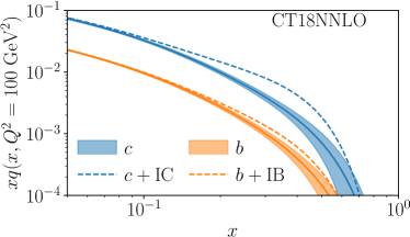
Figure 1: Intrinsic charm and bottom PDFs. The baseline PDFs are from the CT18NNLO PDF set [4]. The shaded regions show the $68\%$ confidence-level regions. The $c+{\rm IC}$ PDF is from CT18FC [3]. The $b+{\rm IB}$ PDF is obtained by scaling the intrinsic component of the CT18FC charm PDF by $m_{c}^{2}/m_{b}^{2}$ and adding the result to the baseline $b$ PDF.

Experimental searches for IC have been carried out in both fixed-target deep-inelastic scattering (DIS) and high-energy hadron collisions. Charm structure function data from the European Muon Collaboration (EMC) experiment [5] and studies of $Z$-boson production in association with charm-quark jets ($Z+c$) by the LHCb experiment [6, 7] are expected to be particularly sensitive probes of IC. The LHCb experiment has also searched for evidence of IC in charm production and charge asymmetry measurements in fixed-target proton-nucleus collisions [8, 9]. Intrinsic heavy flavor is typically characterized by the average momentum carried by the intrinsic heavy quarks, $\left<x\right>_{\rm IC,IB}$, at an initial energy scale $Q_{0}=m_{c}$. The NNPDF collaboration performed a global analysis including EMC and LHCb $Z+c$ data [10]. The analysis claimed $3\sigma$ evidence for nonzero IC with $\left<x\right>_{\rm IC}\approx 1\%$. A global analysis based on the CT18 PDF fit omitted the the LHCb and EMC measurements due to difficulties with theoretical interpretation. The resulting fit mildly prefers nonzero IC, with $\left<x\right>_{\rm IC}\approx 0.5\%$[3]. Yet another global analysis excluded percent-level IC at the $4\sigma$ level [2]. The Electron-Ion Collider (EIC), under construction at Brookhaven National Laboratory, is expected to produce in excess of 100 times more data than previous collider DIS facilities, allowing for detailed studies of the charm quark PDF [11]. Recent studies indicate that the EIC will be able to conclusively observe or exclude percent-level IC in the proton [12, 13].

In contrast to the experimental and theoretical interest in IC, the possibility of intrinsic bottom quarks in the proton has received relatively little attention (see Ref. [14] for a review). The size of the intrinsic heavy-quark contribution to the proton PDF is expected to scale as $1/m_{Q}^{2}$, where $m_{Q}$ is the heavy quark mass, suppressing IB by an order of magnitude relative to IC [15]. As a result, both the absolute size of the IB contribution and its size relative to the perturbative $b$-quark PDF are smaller than the analagous IC contributions. The $b$-hadron cross section in DIS is also suppressed relative to the $c$-hadron cross section due to the smaller electric charge of the $b$ quark. Additionally, the largest $b$-hadron branching fractions to fully reconstructible final states are $\mathcal{O}(10^{-3})$ [16]. As a result of these limitations, little data constraining the $b$-quark PDF exists. What little data does exist does not probe the valence region, leaving the IB content of the proton almost entirely unconstrained [17]. Consequently, no global analysis of IB in the proton has been performed.

The experimental challenges of studying $b$-hadron production in DIS can be partially overcome by using the topology of heavy-flavor hadron decays. This strategy was used by both the H1 and ZEUS experiments at HERA, which used displaced tracks and secondary vertices to identify $b$-hadrons and extract the $b\overline{b}$ contribution to the proton structure function, $F_{2}^{b\overline{b}}$ [17, 18, 19]. The LHC experiments use a similar strategy to identify heavy-flavor jets. Jets containing heavy-flavor hadrons are identified using the properties of displaced charged-particle vertices [20, 21, 22, 23]. Using this strategy, the LHCb experiment is able to identify or “tag” about $60\%$ of jets containing $b$-hadrons and distinguish between $b$ and $c$ jets. The proposed detector at the EIC is expected to have vertex reconstruction capabilities similar to those of LHCb, enabling a similar strategy for tagging heavy-flavor DIS events [11]. Previous studies have explored the performance of topological charm tagging at the EIC, but studies involving $b$ hadrons have focused on using fully reconstructed decays to study hadronization [24]. Previously explored charm tagging methods rely on the ability to identify charged kaons or count displaced tracks, either in the entire event or clustered into jets [25, 26, 27]. In contrast, the algorithm employed by LHCb does not require particle identification and relies only on the topological properties of charged particle vertices.

This paper demonstrates how the LHCb experiment’s jet tagging strategy can be applied to study heavy-flavor production at the EIC. Because the LHCb jet-tagging algorithm depends only on the properties of the heavy flavor decay and not on the jet itself, the algorithm can be naturally adapted to identifying heavy-flavor events in DIS. Section II describes the simulation setup used for these studies, and Section III describes the heavy-flavor tagging algorithm. Section IV presents the expected sensitivity to IB, and Section V summarizes conclusions and discusses additional uses for topological heavy-flavor tagging at the EIC.

II Simulation

The tagging algorithm performance studies were conducted using simulated $e+p$ DIS events generated using the PYTHIA 8.3 generator [28]. The simulation includes both neutral- and charged-current DIS, although the charged-current contribution to the simulated samples is negligible. Simulations were performed for four beam energy configurations: $5\times 100$, $10\times 100$, $10\times 275$, and $18\times 275~{}{\rm GeV}$, where the first number of each pair is the electron energy and the second is the proton energy. These configurations correspond to $\sqrt{s}=45$, $63$, $105$, and $141~{}{\rm GeV}$, respectively. Heavy-flavor events are defined by the presence of a heavy-flavor hadron. A $b$ event contains a $b$ hadron, whereas a $c$ event contains a $c$ hadron and no $b$ hadron. A light-parton ($uds$) event contains no $c$ or $b$ hadrons.

The tagging algorithm’s performance was studied as a function of the kinematic variables $x$ and $Q^{2}$. These variables can be used to calculate the inelasticity $y=Q^{2}/(xs)$. The accessible kinematic region of interest for IB is $Q^{2}>100~{}{\rm GeV}^{2}$ and $x>0.1$. For the beam configurations used in this study, this kinematic region corresponds to $0.01\lesssim y\lesssim 0.5$, a region where the EIC detector is expected to determine $x$ and $Q^{2}$ from the scattered electron with high precision [30]. As a result, $x$ and $Q^{2}$ were determined at parton level for this study. Furthermore, radiative corrections are expected to be less significant for heavy-quark production than for inclusive DIS and were ignored in this study [27].

The response of a hypothetical EIC detector is modeled according to parameterizations based on the expected performance of the future detector [11]. The momentum and position resolutions are given as functions of transverse momentum ($p_{\rm T}$) and pseudorapidity ($\eta$), as shown in Table 1. Only long-lived charged particles with $p_{\rm T}>200~{}{\rm MeV}$ and $|\eta|<2.5$ were considered for this study. A charged particle reconstruction efficiency of $90\%$ was assumed for the entire fiducial region.

The position of the collision vertex, or primary vertex (PV), is determined by smearing the true position of the interaction point. The PV resolution is shown in Ref. [13] and estimated here as $\sigma_{x,y,z}=(10\oplus 30/\sqrt{n})$, where $n$ is the number of reconstructed prompt charged particles. Reconstructed particles are classified as prompt based on

$$\chi^{2}_{\rm DCA,IP}=\frac{d_{x}^{2}}{\sigma_{x}^{2}}+\frac{d_{y}^{2}}{\sigma_{y}^{2}},$$ (1)

where $d_{x,y}$ is the distance of closest approach of the smeared charged particle to the interaction point in the dimension denoted by the subscript, and $\sigma_{x,y}$ is the corresponding detector resolution determined using the parameterizations from Table 1. Tracks are considered prompt if $\chi^{2}_{\rm DCA,IP}<12$.

Table 1: Resolution functions used to smear the generated charged particles to simulate the EIC detector’s response. Both $p$ and $p_{\rm T}$ are in GeV.

	$\sigma_{p}/p$	$\sigma_{xy}$	$\sigma_{z}$
$|\eta|<1$	$0.04p\oplus 1\%$	$30/p_{\rm T}\oplus 5~{}{\rm\mu m}$	$30/p_{\rm T}\oplus 5~{}{\rm\mu m}$
$|\eta|<2.5$	$0.04p\oplus 2\%$	$40/p_{\rm T}\oplus 10~{}{\rm\mu m}$	$100/p_{\rm T}\oplus 20~{}{\rm\mu m}$

III Tagging algorithm

The tagging algorithm used for this study is based on the algorithm described in Ref. [20]. The LHCb algorithm constructs secondary vertices (SVs) within jets and uses two boosted decision tree (BDT) classifiers to identify vertices from light-, $c$-, and $b$-hadron decays. One BDT is trained to distinguish heavy-flavor SVs from light-hadron SVs, and the other is trained to distinguish between $b$ and $c$ SVs. For this study, the LHCb SV reconstruction algorithm was adapted to the simulated EIC data. Heavy-vs.-light and $b$-vs.-$c$ BDTs were trained for a hypothetical EIC detector using variables similar to those used to train the LHCb BDTs.

First, displaced pseudo-reconstructed charged particles are combined to form two-track SVs. Charged particle displacement is characterized by $\chi^{2}_{\rm DCA}$, which is defined as in Eqn. 1 but with distances calculated with respect to the smeared PV position instead of the true interaction point. Charged particles are considered displaced if $\chi^{2}_{\rm DCA}>16$. Pairs of displaced charged particles with a distance of closest approach to one another less than $0.2~{}{\rm mm}$ are combined to form two-track SVs. Next, pairs of two-track SVs that share a track are combined to form three-track SVs. Only SVs with $0.4<m<5.3~{}{\rm GeV}$ are considered for merging, where $m$ is the SV mass calculated assuming the charged pion mass for each of the constituent tracks. This merging process is repeated until no SVs share tracks. The resulting SVs can consist of any number of tracks.

To suppress contributions from strange particle decays, two-track SVs are required to have $m>0.6~{}{\rm GeV}$. This requirement removes both $K^{0}_{\rm s}\to\pi^{+}\pi^{-}$ and $\Lambda\to p\pi^{-}$ decays. Events containing at least one SV passing these requirements are considered tagged. If an event contains multiple SVs, the SV with the largest $p_{\rm T}$ is used for further classification.

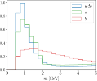
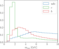
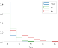
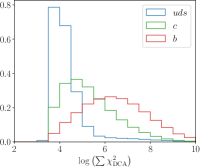
Figure 2: Distributions of variables used for BDT training from the $\sqrt{s}=63~{}{\rm GeV}$ simulated data sample. Each distribution is normalized to unit area.

Tagged events are classified using a pair of BDT classifiers. The first BDT is trained to distinguish heavy-flavor events from $uds$ events (${\rm BDT}_{bc|uds}$), and the second is trained to distinguish between $b$ and $c$ events (${\rm BDT}_{b|c}$). The BDTs use four variables characterizing the SV tag. These include the mass of the SV ($m$), the number of tracks used to construct the SV ($n_{\rm trks}$), and the sum of the $\chi^{2}_{\rm DCA}$ of the constituent tracks. In addition, the BDTs use the corrected mass of the SV, which is given by

$$m_{\rm cor}=\sqrt{m^{2}+p_{\perp}^{2}}+p_{\perp},$$ (2)

where $p_{\perp}$ is the component of the SV momentum perpendicular to its flight direction [31, 32]. These variables are chosen because they depend only on the topological properties of the SV and do not depend on the full SV covariance matrix, which is difficult to estimate without a realistic detector simulation and reconstruction algorithms.

The distributions of the BDT input variables are shown in Fig. 2 for the $\sqrt{s}=63~{}{\rm GeV}$ beam configuration. Bottom hadrons are more massive and produce more final-state particles than $c$ hadrons, which results in the observed hierarchies in $m$ and $n_{\rm trks}$. They also have a longer lifetime than $c$ and light hadrons and consequently have larger $\sum\chi^{2}_{\rm DCA}$. The corrected mass is particularly powerful for identifying $c$ events because $c$ hadrons typically decay at a single vertex. These decays produce a $m_{\rm cor}$ peak near the mass of the $D$ meson. Bottom hadrons produce more complex decay topologies and a consequently broader $m_{\rm cor}$ distribution than that of charm hadrons. SVs in $uds$ events are made up of combinations of poorly-reconstructed prompt tracks. The momenta of these combinations can point far from the PV and produce large corrected masses.

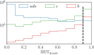
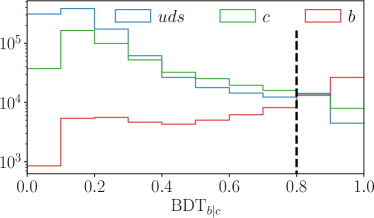
Figure 3: Response distributions for (top) ${\rm BDT}_{bc|uds}$ and (bottom) ${\rm BDT}_{b|c}$ from $\sqrt{s}=63~{}{\rm GeV}$ simulation with expected relative normalizations. The dashed lines show the low edges of the signal regions.

The BDT response distributions are shown in Fig. 3. In an analysis of real data, the composition of the tagged sample could be determined using a two-dimensional template fit to these distributions [33, 34]. For this study, the region ${\rm BDT}_{bc|uds}>0.9$ and ${\rm BDT}_{b|c}>0.8$ was defined as the signal region (SR) for the purpose of estimating statistical uncertainties. The signal region tagging efficiency $\epsilon_{\rm SR}$, defined as the probability that an event is tagged and the SV falls in the BDT SR, is shown in Fig. 4 for the $\sqrt{s}=63~{}{\rm GeV}$ configuration. The tagging efficiency ranges from $30\mbox{--}40\%$ in most kinematically allowed bins and approaches $60\%$ at high $Q^{2}$. This efficiency is consistent with the $b$-jet tagging efficiency observed by LHCb, which approached $60\%$ at high jet $p_{\rm T}$. Charm events have a signal-region mistag probability of around $1\%$, while $uds$ events have a mistag probability of around $10^{-4}$. While $uds$ events are the largest background overall, their contribution to the signal region is small. The fast simulation used in this study does not include non-Gaussian misreconstruction effects or secondary particle production from material interactions. Both of these effects will create additional SVs in $uds$ events, but these SVs should still be distinguishable from heavy flavor decays and are expected to make a small contribution to the signal region [20].

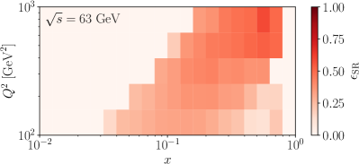
Figure 4: The signal region tagging efficiency determined from $\sqrt{s}=63~{}{\rm GeV}$ simulation. Kinematically forbidden regions are given an efficiency of zero.

IV Intrinsic bottom

The $b\overline{b}$ production cross section in unpolarized neutral-current DIS in the kinematic region studied here is given by

$$\frac{{\rm d}\sigma^{b{\overline{b}}}}{{\rm d}x{\rm d}Q^{2}}=\frac{2\pi\alpha^{2}Y_{+}}{xQ^{4}}\left(F^{b\overline{b}}_{2}(x,Q^{2})-\frac{y^{2}}{Y_{+}}F^{b\overline{b}}_{L}(x,Q^{2})\right),$$ (3)

where $\alpha$ is the fine structure constant, $Y_{+}=1+(1-y)^{2}$, and $F^{b\overline{b}}_{2}$ and $F^{b\overline{b}}_{L}$ are the $b$-quark contributions to the proton structure functions [17]. DIS experiments typically report a reduced cross section given by

$$\sigma^{b\overline{b}}_{r}(x,Q^{2})=F^{b\overline{b}}_{2}(x,Q^{2})-\frac{y^{2}}{Y_{+}}F^{b\overline{b}}_{L}(x,Q^{2}).$$ (4)

For the relatively small values of $y$ considered in this study, $\sigma^{b\overline{b}}_{r}$ is determined primarily by $F^{b\overline{b}}_{2}$. At leading order (LO) in the strong coupling constant $\alpha_{\rm s}$, $F^{b\overline{b}}_{2}$ is proportional to the sum of $b$ and $\overline{b}$ PDFs.

The estimate of the IB contribution to $\sigma^{b\overline{b}}_{r}$ is based on two observations. First, the intrinsic heavy quark PDFs evolve approximately independently from the other PDFs [15]. This means that the IC contribution to the charm PDF can be approximated as $c_{0+{\rm IC}}(x,Q^{2})-c_{0}(x,Q^{2})$, where $c_{0}$ is the charm PDF from a fit without IC and $c_{0+{\rm IC}}$ is from a fit that includes IC. The intrinsic $b$ PDF can then be estimated as

$$b_{\rm IB}(x,Q^{2})=\frac{m_{c}^{2}}{m_{b}^{2}}\left(c_{0+{\rm IC}}(x,Q^{2})-c_{0}(x,Q^{2})\right).$$ (5)

Second, the dominant contribution from intrinsic heavy quarks to the reduced cross section is from the LO contribution to $F_{2}^{q\overline{q}}$. As a result,

$$\sigma^{b\overline{b}}_{r,{\rm IB}}(x,Q^{2})\approx\sigma^{b\overline{b}}_{r{\rm no\mbox{-}IB}}(x,Q^{2})+2e_{b}^{2}xb_{\rm IB}(x,Q^{2}),$$ (6)

where $\sigma^{b\overline{b}}_{r{\rm no\mbox{-}IB}}$ is the reduced cross section section assuming no IB, and $e_{b}$ is the electric charge of the $b$ quark. The factor of two in front of the IB term accounts for the $\overline{b}$ contribution, assuming the $b$ and $\overline{b}$ PDFs are symmetric. Applying this strategy to calculate $\sigma^{c\overline{c}}_{r{\rm IC}}$ reproduces the full next-to-next-to-leading order (NNLO) result to within about 10% in the kinematic region covered by this study, which is sufficiently accurate for the sensitivity estimates performed here. Consequently, the IB contribution can be estimated using only $c_{0}$, $c_{0+{\rm IC}}$, and $\sigma^{b\overline{b}}_{r{\rm no\mbox{-}IB}}$.

The no-IB cross sections for $b$, $c$, and $uds$ events were calculated at NNLO in $\alpha_{\rm s}$ using the Yadism package [35]. The calculations were performed using the zero-mass variable flavor number scheme (ZM-VFNS) and the CT18NNLO PDF set, which was accessed using LHAPDF [4, 36]. The no-IC charm PDF $c_{0}$ is taken from CT18NNLO, and $c_{0+{\rm IC}}$ was taken from CT18FC [3]. CT18FC includes IC using the LFQCD-inspired model of Ref. [1] with $\left<x\right>_{\rm IC}\approx 0.5\%$. It should be noted that the IC PDF from CT18FC is smaller than that from other global analyses, and IC normalizations almost three times larger than that used for this study are allowed within the CT18FC $68\%$ confidence interval. Furthermore, the $m_{c}^{2}/m_{b}^{2}$ IB scaling is unconfirmed. IB with an order-of-magnitude larger overall normalization has not been excluded by data[15]. In this sense, the IB model used in this study is conservative.

The cross sections are used to calculate expected yields from one year of data taking in each beam configuration according to the integrated luminosities given in Refs. [30] and [37], which are reproduced in Table 2. Signal-region tagging efficiencies for $b$, $c$, and $uds$ events were calculated for each beam configuration as described in Sec. III and were used to calculate expected tagged yields. The tagged yields were then used to determine signal significance and expected statistical uncertainties. The IC contribution to the $c\overline{c}$ cross section is included as background in the IB predictions.

Table 2: Expected annual integrated luminosities for various EIC beam configurations.

$\sqrt{s}~{}[{\rm GeV}]$	$\mathcal{L}_{\rm int}/{\rm year}~{}[{\rm fb}^{-1}]$
$45$	61.0
$63$	79.0
$105$	100.0
$141$	15.4

The $\sigma_{r,{\rm IB}}^{b\overline{b}}$ results are shown in Fig. 5. To better illustrate the estimated sensitivity to IB, the ratio of the IB results to the baseline are shown in Fig. 6. IB produces an enhancement of up to a factor of $3$ in the valence region. The enhancement is most pronounced at low $Q^{2}$, where the contribution from perturbative $b$ is smallest. In most of the kinematic bins where IB has a significant effect, the $b$ PDF uncertainties are much larger than the expected statistical uncertainties. Because the no-IB PDF is determined entirely from gluon splitting via DGLAP evolution, these PDF uncertainties reflect uncertainties in the gluon PDF at high $x$. Consequently, the EIC’s sensitivity to IB will depend in part on future constraints on the high-$x$ gluon PDF from both the EIC and the LHC.

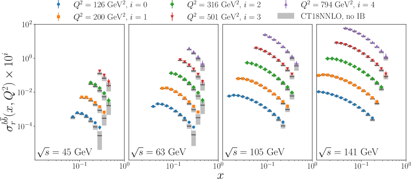
Figure 5: Reduced cross section predictions. The points show predictions with IB, and the errorbars show expected statistical uncertainties. The black lines show predictions without IB, and the shaded boxes show the $68\%$ confidence-level PDF uncertainties. For visual clarity, the result in each $Q^{2}$ bin is offset by a factor $10^{i}$, shown in the legend.

Using LHCb’s experience as a guide, the largest systematic uncertainties for measurements using this tagging algorithm are likely to arise from the tagging efficiency determination and the BDT template calibration. The LHCb experiment was able to measure its jet tagging efficiency in data to within about 10% and calibrate its templates using dijet calibration samples [21, 20]. A similar calibration is possible for $c\overline{c}$ events at the EIC using SV-tagged events containing a fully reconstructed $D^{0}\to K^{-}\pi^{+}$ decay with a large separation in azimuthal angle $\phi$ from the tagging SV. The $b$ tagging performance can be studied using events containing two $b$-like tags with large separations in $\phi$. Ultimately, because the same templates are used for efficiency determinations and signal yield extraction, these uncertainties partially cancel in actual measurements. Furthermore, the remaining uncertainty will likely be highly correlated across kinematic bins and should only mildly affect sensitivity to IB. Measurements of heavy flavor production by the H1 and ZEUS collaborations using topological tagging also found that the dominant systematic uncertainties were highly correlated between data points [18, 19].

The search for IB will also be complicated by the handling of the $b$-quark mass in the $b$ PDF evolution. The $b$-quark pole mass is typically used as a starting scale for generating $b$ quarks perturbatively and is anticorrelated with the $b$ PDF. Variations of $m_{b}$ within its uncertainties can produce changes in the $b$ PDF comparable to the PDF fit uncertainties in the valence region [38, 39]. Varying $m_{b}$ has a much larger effect at low $x$, however, and data over the broad $x$ range studied here would provide strong constraints on both IB and $m_{b}$ simultaneously. This data would also provide powerful tests of the heavy-quark scheme used in structure function calculations [40].

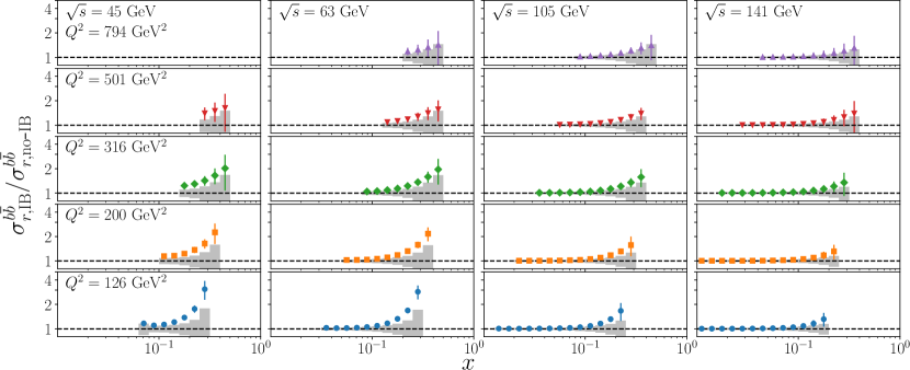
Figure 6: Ratio of the $b\overline{b}$ reduced cross section with IB to the no IB case. The shaded regions show the $68\%$ confidence interval PDF uncertainties for the no-IB case.

V Conclusions

Topological $b$ tagging has proven to be a powerful tool for studying QCD in high-energy hadron collisions, and this work demonstrates that these methods are directly applicable to the EIC. The tagging strategy described here has a wide range of potential applications in electron-proton and electron-nucleus scattering. This algorithm could be used to tag heavy-flavor jets, which can be used to study both the structure of nuclei and the hadronization process [25, 41]. It could also be used to study heavy dihadron angular correlations, which provide sensitivity to gluon transverse momentum distributions[42, 26]. This tagging strategy can also be used to efficiently tag charm events, potentially expanding the kinematic reach of charm production measurements at the EIC.

This paper also presents the first study of the EIC’s ability to probe the $b$-quark PDF and its sensitivity to intrinsic bottom quarks. The EIC has the potential to observe intrinsic bottom at levels expected from recent global analyses of intrinsic charm in the proton. The observation of intrinsic bottom quarks is crucial for understanding the origin of intrinsic heavy quarks, including possible nonperturbative processes that produce heavy quarks in protons and nuclei. This paper presents the first strategy for observing intrinsic bottom in the near future.

References

- Brodsky et al. [1980] S. J. Brodsky, P. Hoyer, C. Peterson, and N. Sakai, Phys. Lett. B93, 451 (1980).
- Hobbs et al. [2014] T. J. Hobbs, J. T. Londergan, and W. Melnitchouk, Phys. Rev. D89, 074008 (2014), arXiv:1311.1578 [hep-ph] .
- Guzzi et al. [2023] M. Guzzi, T. J. Hobbs, K. Xie, J. Huston, P. Nadolsky, and C. P. Yuan, Phys. Lett. B843, 137975 (2023), arXiv:2211.01387 [hep-ph] .
- Hou et al. [2021] T.-J. Hou et al., Phys. Rev. D103, 014013 (2021), arXiv:1912.10053 [hep-ph] .
- Aubert et al. [1983] J. J. Aubert et al. (European Muon), Nucl. Phys. B213, 31 (1983).
- Aaij et al. [2022a] R. Aaij et al. (LHCb), Phys. Rev. Lett. 128, 082001 (2022a), arXiv:2109.08084 [hep-ex] .
- Boettcher et al. [2016] T. Boettcher, P. Ilten, and M. Williams, Phys. Rev. D93, 074008 (2016), arXiv:1512.06666 [hep-ph] .
- Aaij et al. [2019] R. Aaij et al. (LHCb), Phys. Rev. Lett. 122, 132002 (2019), arXiv:1810.07907 [hep-ex] .
- Aaij et al. [2023] R. Aaij et al. (LHCb), Eur. Phys. J. C83, 541 (2023), arXiv:2211.11633 [hep-ex] .
- Ball et al. [2022] R. D. Ball, A. Candido, J. Cruz-Martinez, S. Forte, T. Giani, F. Hekhorn, K. Kudashkin, G. Magni, and J. Rojo (NNPDF), Nature 608, 483 (2022), arXiv:2208.08372 [hep-ph] .
- Abdul Khalek et al. [2022] R. Abdul Khalek et al., Nucl. Phys. A1026, 122447 (2022), arXiv:2103.05419 [physics.ins-det] .
- Ball et al. [2023] R. D. Ball, A. Candido, J. Cruz-Martinez, S. Forte, T. Giani, F. Hekhorn, G. Magni, E. R. Nocera, J. Rojo, and R. Stegeman (NNPDF), (2023), arXiv:2311.00743 [hep-ph] .
- Kelsey et al. [2021] M. Kelsey, R. Cruz-Torres, X. Dong, Y. Ji, S. Radhakrishnan, and E. Sichtermann, Phys. Rev. D104, 054002 (2021), arXiv:2107.05632 [hep-ph] .
- Brodsky et al. [2015] S. J. Brodsky, A. Kusina, F. Lyonnet, I. Schienbein, H. Spiesberger, and R. Vogt, Adv. High Energy Phys. 2015, 231547 (2015), arXiv:1504.06287 [hep-ph] .
- Lyonnet et al. [2015] F. Lyonnet, A. Kusina, T. Ježo, K. Kovarík, F. Olness, I. Schienbein, and J.-Y. Yu, JHEP 07, 141, arXiv:1504.05156 [hep-ph] .
- Workman et al. [2022] R. L. Workman et al. (Particle Data Group), PTEP 2022, 083C01 (2022).
- Abramowicz et al. [2018] H. Abramowicz et al. (H1, ZEUS), Eur. Phys. J. C78, 473 (2018), arXiv:1804.01019 [hep-ex] .
- Aaron et al. [2010] F. D. Aaron et al. (H1), Eur. Phys. J. C65, 89 (2010), arXiv:0907.2643 [hep-ex] .
- Abramowicz et al. [2014] H. Abramowicz et al. (ZEUS), JHEP 09, 127, arXiv:1405.6915 [hep-ex] .
- Aaij et al. [2015a] R. Aaij et al. (LHCb), JINST 10 (06), P06013, arXiv:1504.07670 [hep-ex] .
- Aaij et al. [2022b] R. Aaij et al. (LHCb), JINST 17 (02), P02028, arXiv:2112.08435 [hep-ex] .
- Aad et al. [2023] G. Aad et al. (ATLAS), Eur. Phys. J. C83, 681 (2023), arXiv:2211.16345 [physics.data-an] .
- Sirunyan et al. [2018] A. M. Sirunyan et al. (CMS), JINST 13 (05), P05011, arXiv:1712.07158 [physics.ins-det] .
- Wong et al. [2020] C.-P. Wong, X. Li, M. Brooks, M. J. Durham, M. X. Liu, A. Morreale, C. da Silva, and W. E. Sondheim, (2020), arXiv:2009.02888 [nucl-ex] .
- Arratia et al. [2021] M. Arratia, Y. Furletova, T. J. Hobbs, F. Olness, and S. J. Sekula, Phys. Rev. D103, 074023 (2021), arXiv:2006.12520 [hep-ph] .
- Dong et al. [2023] X. Dong, Y. Ji, M. Kelsey, S. Radhakrishnan, E. Sichtermann, and Y. Zhao, Phys. Rev. D107, 074022 (2023), arXiv:2210.08609 [hep-ph] .
- Aschenauer et al. [2017] E. C. Aschenauer, S. Fazio, M. A. C. Lamont, H. Paukkunen, and P. Zurita, Phys. Rev. D96, 114005 (2017), arXiv:1708.05654 [nucl-ex] .
- Bierlich et al. [2022] C. Bierlich et al., SciPost Phys. Codeb. 2022, 8 (2022), arXiv:2203.11601 [hep-ph] .
- Note [1] Natural units are used throughout this paper.
- Armesto et al. [2023] N. Armesto, T. Cridge, F. Giuli, L. Harland-Lang, P. Newman, B. Schmookler, R. Thorne, and K. Wichmann, (2023), arXiv:2309.11269 [hep-ph] .
- Williams et al. [2011] M. Williams, V. Gligorov, C. Thomas, H. Dijkstra, J. Nardulli, and P. Spradlin, (2011).
- Abe et al. [1998] K. Abe et al. (SLD), Phys. Rev. Lett. 80, 660 (1998), arXiv:hep-ex/9708015 .
- Aaij et al. [2015b] R. Aaij et al. (LHCb), Phys. Rev. D92, 052001 (2015b), arXiv:1505.04051 [hep-ex] .
- Aaij et al. [2015c] R. Aaij et al. (LHCb), Phys. Rev. Lett. 115, 112001 (2015c), arXiv:1506.00903 [hep-ex] .
- Candido et al. [2024] A. Candido, F. Hekhorn, G. Magni, T. R. Rabemananjara, and R. Stegeman, (2024), arXiv:2401.15187 [hep-ph] .
- Buckley et al. [2015] A. Buckley, J. Ferrando, S. Lloyd, K. Nordström, B. Page, M. Rüfenacht, M. Schönherr, and G. Watt, Eur. Phys. J. C75, 132 (2015), arXiv:1412.7420 [hep-ph] .
- Cerci et al. [2023] S. Cerci, Z. S. Demiroglu, A. Deshpande, P. R. Newman, B. Schmookler, D. Sunar Cerci, and K. Wichmann, Eur. Phys. J. C83, 1011 (2023), arXiv:2307.01183 [hep-ph] .
- Cridge et al. [2021] T. Cridge, L. A. Harland-Lang, A. D. Martin, and R. S. Thorne, Eur. Phys. J. C81, 744 (2021), arXiv:2106.10289 [hep-ph] .
- Campbell et al. [2021] J. Campbell, T. Neumann, and Z. Sullivan, Phys. Rev. D104, 094042 (2021), arXiv:2109.10448 [hep-ph] .
- Accardi et al. [2016] A. Accardi et al., Eur. Phys. J. C76, 471 (2016), arXiv:1603.08906 [hep-ph] .
- Li et al. [2022] H. T. Li, Z. L. Liu, and I. Vitev, Phys. Lett. B827, 137007 (2022), arXiv:2108.07809 [hep-ph] .
- del Castillo et al. [2022] R. F. del Castillo, M. G. Echevarria, Y. Makris, and I. Scimemi, JHEP 03, 047, arXiv:2111.03703 [hep-ph] .