Between- and Within-Cluster Spearman Rank Correlations

Abstract

Clustered data are common in practice. Clustering arises when subjects are measured repeatedly, or subjects are nested in groups (e.g., households, schools). It is often of interest to evaluate the correlation between two variables with clustered data. There are three commonly used Pearson correlation coefficients (total, between-, and within-cluster), which together provide an enriched perspective of the correlation. However, these Pearson correlation coefficients are sensitive to extreme values and skewed distributions. They also depend on the scale of the data and are not applicable to ordered categorical data. Current non-parametric measures for clustered data are only for the total correlation. Here we define population parameters for the between- and within-cluster Spearman rank correlations. The definitions are natural extensions of the Pearson between- and within-cluster correlations to the rank scale. We show that the total Spearman rank correlation approximates a weighted sum of the between- and within-cluster Spearman rank correlations, where the weights are functions of rank intraclass correlations of the two random variables. We also discuss the equivalence between the within-cluster Spearman rank correlation and the covariate-adjusted partial Spearman rank correlation. Furthermore, we describe estimation and inference for the three Spearman rank correlations, conduct simulations to evaluate the performance of our estimators, and illustrate their use with data from a longitudinal biomarker study and a clustered randomized trial.

Keywords: Clustered data; Rank association measures; Spearman rank correlation

1 Introduction

Clustered data are common in practice. Clustering arises when subjects (e.g., people) are measured repeatedly, or subjects are nested in clusters (e.g., households, schools) and measured only once. The total, between-, and within-cluster Pearson correlations are frequently used in the analysis of clustered data (Snijders and Bosker, 1999; Ferrari et al., 2005). The total correlation measures the overall correlation but fails to acknowledge the clustered nature of the data. The between-cluster correlation measures the association between underlying variables at the cluster level, while the within-cluster correlation is the correlation after controlling for clustering.

For example, in an observational study, people living with HIV on antiretroviral therapy (ART) had repeated measurements of CD4 and CD8 counts (Castilho et al., 2016). There is interest in measuring the correlation between CD4 and CD8 counts subject to clustering. The between-cluster correlation measures the association between the underlying CD4 and CD8 counts in individuals. The within-cluster correlation describes the correlation between variations in CD4 and CD8 measures due to changes over time or measurement errors. Together, the total, between-, and within-cluster correlations provide a more complete picture of the relationship between CD4 and CD8 counts.

However, Pearson correlations are sensitive to extreme values and skewed distributions, and they depend on the scale of the data. For example, CD4 and CD8 counts are both right-skewed and sometimes transformed prior to analyses; estimates of the total, between-, and within-cluster Pearson correlations will vary with the transformation. Some recent studies have proposed nonparametric measures of correlation for clustered data. Rosner and Glynn (2017) proposed a regression-based approach to obtain the maximum likelihood estimate of Pearson correlation for clustered data and then compute Spearman rank correlation by using its relationship with Pearson correlation under bivariate normality. Shih and Fay (2017) defined Spearman rank correlation for clustered data as the Pearson correlation between the population versions of ridits (Bross, 1958), and applied within-cluster resampling and U-statistics for estimation and inference. Hunsberger, et al (2022) extended the work of Shih and Fay by improving the nominal level of the tests for clustered data with small sample sizes. However, these nonparametric measures are only for the total correlation. There is a need to develop rank-based between- and within-cluster correlations.

In this paper, we define population parameters of between- and within-cluster Spearman rank correlations, which are natural extensions of the traditional between- and within-cluster Pearson correlations to the rank scale. We show that the total Spearman rank correlation approximates a weighted sum of the between- and within-cluster Spearman rank correlations, where the weights are functions of rank intraclass correlation coefficients (Tu et al., 2023). We also show the equivalence between the within-cluster Spearman’s rank correlation and the covariate-adjusted partial Spearman’s rank correlation with cluster indicators as covariates (Liu et al., 2018).

This paper is organized as follows. In Section 2, we briefly review Pearson correlations for clustered data. In Section 3, we introduce population parameters of the total, between-, and within-cluster Spearman rank correlations for clustered data. In Section 4, we illustrate the relationship between the three Spearman rank correlations. In Sections 5 and 6, we describe estimation and inference using semiparametric cumulative probability models. In Section 7, we conduct simulations to evaluate the performance of our estimators under different scenarios. In Section 8, we illustrate our method in two applications: a clustered randomized trial and a longitudinal biomarker study. Section 9 provides a discussion. Additional information is in the Supplementary Materials.

2 Review of Pearson correlations for clustered data

Let $X_{ij}$ and $Y_{ij}$ denote two random variables from a two-level hierarchical joint distribution, where $i$ represents cluster and $j$ is the index within cluster $i$. For the review in this section, we assume an additive model and equal within-cluster covariance matrices across clusters. Specifically, consider a bivariate population model of $(X_{ij},Y_{ij})^{T}$ in an infinite population,

$$\begin{pmatrix}X_{ij}\\ Y_{ij}\end{pmatrix}=\begin{pmatrix}U_{Xi}\\ U_{Yi}\end{pmatrix}+\begin{pmatrix}R_{Xij}\\ R_{Yij}\end{pmatrix},$$ (1)

where $(U_{Xi},U_{Yi})^{T}$ is the cluster mean of the $i$th cluster, $(R_{Xij},R_{Yij})^{T}$ is the within-cluster deviation of the $j$th observation in the $i$th cluster with zero means, and $(U_{Xi},U_{Yi})^{T}\perp(R_{Xij},R_{Yij})^{T}$. The covariance matrix of $(U_{Xi},U_{Yi})^{T}$ is denoted as $\begin{pmatrix}\sigma^{2}_{u}&\rho_{b}\sigma_{u}\eta_{u}\\ \rho_{b}\sigma_{u}\eta_{u}&\eta_{u}^{2}\end{pmatrix}$, and the covariance matrix of $(R_{Xij},R_{Yij})^{T}$ is denoted as $\begin{pmatrix}\sigma^{2}_{r}&\rho_{w}\sigma_{r}\eta_{r}\\ \rho_{w}\sigma_{r}\eta_{r}&\eta_{r}^{2}\end{pmatrix}$. The intraclass correlation coefficient (ICC) of $X$ is $\rho_{I_{X}}=\sigma^{2}_{u}/(\sigma^{2}_{u}+\sigma^{2}_{r})$ and of $Y$ is $\rho_{I_{Y}}=\eta^{2}_{u}/(\eta^{2}_{u}+\eta^{2}_{r})$, evaluating the correlation between two random observations in a random cluster.

With the above bivariate population model, the between-cluster correlation is the correlation between the cluster means, $\rho_{b}=corr(U_{Xi},U_{Yi})$. The within-cluster correlation is the correlation between the within-cluster deviations, $\rho_{w}=corr(R_{Xij},R_{Yij})$. Since

$$\rho_{t} =\rho(X_{ij},Y_{ij})$$

$$=\frac{\text{cov}(X_{ij},Y_{ij})}{\sqrt{\text{var}(X_{ij})\text{var}(Y_{ij})}}$$

$$=\frac{\text{cov}(U_{Xi},U_{Yi})+\text{cov}(R_{Xij},R_{Yij})}{\sqrt{\text{var}(X_{ij})\text{var}(Y_{ij})}}$$

$$=\frac{\rho_{b}\sigma_{u}\eta_{u}+\rho_{w}\sigma_{r}\eta_{r}}{\sqrt{(\sigma^{2}_{u}+\sigma^{2}_{r})(\eta^{2}_{u}+\eta^{2}_{r})}}$$

$$=\rho_{b}\sqrt{\rho_{I_{X}}\rho_{I_{Y}}}+\rho_{w}\sqrt{(1-\rho_{I_{X}})(1-\rho_{I_{Y}})},$$ (2)

the total correlation is a weighted sum of the between- and within-cluster correlations, where the weights depend on the ICCs of $X$ and $Y$.

3 Population parameters of Spearman rank correlations for clustered data

Spearman rank correlation is essentially the correlation between cumulative distribution functions (CDFs) for continuous variables, also known as the grade correlation (Kruskal, 1958), or more broadly, the correlation between population versions of midranks or ridits (Kendall, 1970; Bross, 1958). Generically, let $F$ be a CDF, $F(x-)=\lim_{t\uparrow x}F(t)$, and $F^{*}(x)=\{F(x)+F(x-)\}/2$. If the distribution is continuous, then $F^{*}(x)=F(x)$. If the distribution is discrete or mixed, $F^{*}(x)$ corresponds to the population versions of ridits (Bross, 1958). The population parameter of Spearman rank correlation between two random variables $X$ and $Y$ with CDFs $F_{X}$ and $F_{Y}$ is denoted as $\gamma(X,Y)=corr\{F^{*}_{X}(X),F^{*}_{Y}(Y)\}$ (Kendall, 1970; Liu et al., 2018).

Let $X_{ij}$ and $Y_{ij}$ denote two random variables from a two-level hierarchical joint distribution, where $i$ represents cluster and $j$ is the index within cluster $i$. The total Spearman rank correlation is the overall rank correlation between $X_{ij}$ and $Y_{ij}$. We define its population parameter as

$$\gamma_{t} =\gamma(X_{ij},Y_{ij})=corr\{F^{*}_{X}(X_{ij}),F_{Y}^{*}(Y_{ij})\}.$$ (3)

With continuous $X_{ij}$ and $Y_{ij}$, $\gamma_{t}=12cov\{F_{X}(X_{ij}),F_{Y}(Y_{ij})\}$, because $F^{*}_{X}(X_{ij})=F_{X}(X_{ij})\sim Unif(0,1)$, $F^{*}_{Y}(Y_{ij})=F_{Y}(Y_{ij})\sim Unif(0,1)$, and their variances equal $1/12$.

Let $F_{X|i}$ and $F_{Y|i}$ be the CDFs of $X$ and $Y$ conditional on being in cluster $i$, respectively. The population parameter of the within-cluster Spearman rank correlation is defined as

$$\gamma_{w} =corr\{F^{*}_{X|i}(X_{ij}),F^{*}_{Y|i}(Y_{ij})\}.$$ (4)

Note that $\gamma_{w}$ is not a function of cluster index and that it does not assume an equal variance structure across clusters. In fact, $\gamma_{w}$ is identical to the covariate-adjusted partial Spearman rank correlation (Liu et al., 2018), where the covariates are cluster indicators. Since the partial Spearman rank correlation can be expressed using probability-scale residuals (PSRs) (Li and Shepherd, 2012; Shepherd et al., 2016), we can express $\gamma_{w}$ similarly. The PSRs of $X_{ij}=x$ and $Y_{ij}=y$ are defined as $r(x,F_{X|i})=2F^{*}_{X|i}(x)-1$ and $r(y,F_{Y|i})=2F^{*}_{Y|i}(y)-1$, respectively. Then we have

$$\gamma_{w}=corr(r(X_{ij},F_{X|i}),r(Y_{ij},F_{Y|i})).$$

This connection allows us to derive an estimator for $\gamma_{w}$, which will be described in Section 5.

The usage of cluster means is not desirable for the between-cluster Spearman rank correlation because means are scale-dependent and sensitive to outliers and skewness. We use the general concept of cluster centroids to define the between-cluster Spearman rank correlation. A cluster centroid defines the central tendency of random variables in the same cluster. It is usually the median. Let $\tilde{X}_{i}$ and $\tilde{Y}_{i}$ be the cluster centroid parameters of the $i$th cluster, with marginal CDFs denoted as $F_{\tilde{X}}$ and $F_{\tilde{Y}}$, respectively. Assuming that clusters are independent, the between-cluster Spearman rank correlation treats clusters as units of interest and measures the association between cluster centroids. We define its population parameter as

$$\gamma_{b} =\gamma(\tilde{X}_{i},\tilde{Y}_{i})=corr\{F^{*}_{\tilde{X}}(\tilde{X}_{i}),F_{\tilde{Y}}^{*}(\tilde{Y}_{i})\}.$$ (5)

Our definitions of $\gamma_{t}$, $\gamma_{b}$, and $\gamma_{w}$ are easily interpreted as rank correlations. In the special case where $(X_{ij},Y_{ij})^{T}$ has a similar hierarchical population model as (1) in Section 2 except that $(U_{Xi},U_{Yi})^{T}$ is the cluster median and $(R_{Xij},R_{Yij})^{T}$ has a median of zero, then $\gamma_{t}=\gamma(X_{ij},Y_{ij})$, $\gamma_{b}=\gamma(U_{Xi},U_{Yi})$, and $\gamma_{w}=\gamma(R_{Xij},R_{Yij})$.

Furthermore, our definitions of $\gamma_{t}$, $\gamma_{b}$, and $\gamma_{w}$ are also applicable to ordered categorical data. While the definitions of $\gamma_{t}$ and $\gamma_{w}$ in (3) and (4) can be directly applied, the definition of $\gamma_{b}$ in (5) needs an extension. For an ordered categorical variable $X$, the median is defined as any category $c$ for which $P(X\leq c)\geq 0.5$ and $P(X\geq c)\geq 0.5$. The median is often a unique value. In the rare situation where $P(X\leq c)=0.5$, both the category $c$ and the next higher category (denoted as $c+$) are the medians, and we define the cluster centroid $\tilde{X}$ as $c$ with a probability of 0.5 and $c+$ with a probability of 0.5. If there are clusters like this with two cluster medians for a variable, we define $\gamma_{b}=E[\gamma(\tilde{X}_{i},\tilde{Y}_{i})]$, the expectation of the Spearman rank correlation over all possible combinations of cluster medians in the population. If no clusters have two cluster medians, the definition in (5) can be directly applied.

4 Relationship between $\gamma_{t}$, $\gamma_{w}$, and $\gamma_{b}$

The total Spearman rank correlation can be decomposed into two weighted components. The weights are functions of the rank ICC, which is a natural extension of Fisher’s ICC (Fisher, 1925) to the rank scale (Tu et al., 2023). The rank ICC of $X$ is

$$\gamma_{I_{X}} =corr[F_{X}^{*}(X_{ij}),F_{X}^{*}(X_{ij^{\prime}})]$$

$$=cov[F^{*}_{X}(X_{ij}),F^{*}_{X}(X_{ij^{\prime}})]/var[F^{*}_{X}(X_{ij})]$$

$$=cov\{E[F^{*}_{X}(X_{ij})|i],E[F^{*}_{X}(X_{ij^{\prime}})|i]\}/var[F^{*}_{X}(X_{ij})]$$

$$\>\>\>\>\>+E\{cov[F^{*}_{X}(X_{ij}),F^{*}_{X}(X_{ij^{\prime}})|i]\}/var[F^{*}_{X}(X_{ij})]$$

$$=var\{E[F^{*}_{X}(X_{ij})|i]\}/var[F^{*}_{X}(X_{ij})]+D_{X},$$

where $(X_{ij},X_{ij^{\prime}})$ is a random pair drawn from a random cluster and $j\neq j^{\prime}$, and $D_{X}=E\{cov[F^{*}_{X}(X_{ij}),F^{*}_{X}(X_{ij^{\prime}})|i]\}/var[F^{*}_{X}(X_{ij})]$. When cluster sizes in the population are finite, $D_{X}$ is negative. When cluster sizes in the population are infinite, $D_{X}$ is equal to 0. The rank ICC of $Y$, $\gamma_{I_{Y}}$, is similarly defined.

The decomposition of the total Spearman rank correlation is

$$\gamma_{t} =corr\{F_{X}^{*}(X_{ij}),F^{*}_{Y}(Y_{ij})\}$$

$$=\frac{cov\{F_{X}^{*}(X_{ij}),F^{*}_{Y}(Y_{ij})\}}{\sqrt{var[F_{X}^{*}(X_{ij})]var[F^{*}_{Y}(Y_{ij})]}}$$

$$=\frac{cov\{E[F_{X}^{*}(X_{ij})|i],E[F^{*}_{Y}(Y_{ij})|i]\}+E\{cov[F_{X}^{*}(X_{ij}),F^{*}_{Y}(Y_{ij})|i]\}}{\sqrt{var[F_{X}^{*}(X_{ij})]var[F^{*}_{Y}(Y_{ij})]}}$$

$$=\frac{cov\{E[F_{X}^{*}(X_{ij})|i],E[F^{*}_{Y}(Y_{ij})|i]\}}{var\{E[F_{X}^{*}(X_{ij})|i]\}var\{E[F^{*}_{Y}(Y_{ij})|i]\}}\sqrt{\frac{var\{E[F^{*}_{X}(X_{ij})|i]\}}{var[F^{*}_{X}(X_{ij})]}}\sqrt{\frac{var\{E[F^{*}_{Y}(Y_{ij})|i]\}}{var[F^{*}_{Y}(Y_{ij})]}}$$

$$+\frac{E\{cov[F_{X}^{*}(X_{ij}),F^{*}_{Y}(Y_{ij})|i]\}}{\sqrt{E\{var[F_{X}^{*}(X_{ij})|i]\}E\{var[F_{Y}^{*}(Y_{ij})|i]\}}}\sqrt{\frac{E\{var[F_{X}^{*}(X_{ij})|i]\}}{var[F^{*}_{X}(X_{ij})]}}\sqrt{\frac{E\{var[F_{Y}^{*}(Y_{ij})|i]\}}{var[F^{*}_{Y}(Y_{ij})]}}$$

$$=corr\{E[F_{X}^{*}(X_{ij})|i],E[F^{*}_{Y}(Y_{ij})|i]\}\sqrt{(\gamma_{I_{X}}-D_{X})(\gamma_{I_{Y}}-D_{Y})}$$

$$+\frac{E\{cov[F_{X}^{*}(X_{ij}),F^{*}_{Y}(Y_{ij})|i]\}}{\sqrt{E\{var[F_{X}^{*}(X_{ij})|i]\}E\{var[F_{Y}^{*}(Y_{ij})|i]\}}}\sqrt{(1-\gamma_{I_{X}}+D_{X})(1-\gamma_{I_{Y}}+D_{Y})}$$

$$=S_{1}\sqrt{(\gamma_{I_{X}}-D_{X})(\gamma_{I_{Y}}-D_{Y})}+S_{2}\sqrt{(1-\gamma_{I_{X}}+D_{X})(1-\gamma_{I_{Y}}+D_{Y})},$$

where $S_{1}=corr\{E[F_{X}^{*}(X_{ij})|i],E[F^{*}_{Y}(Y_{ij})|i]\}$ and $S_{2}=\frac{E\{cov[F_{X}^{*}(X_{ij}),F^{*}_{Y}(Y_{ij})|i]\}}{\sqrt{E[var[F_{X}^{*}(X_{ij})|i]E[var[F_{Y}^{*}(Y_{ij})|i]}}$. When the cluster size in the population is infinite, then $D_{X}=D_{Y}=0$ and $\gamma_{t}=S_{1}\sqrt{\gamma_{I_{X}}\gamma_{I_{Y}}}+S_{2}\sqrt{(1-\gamma_{I_{X}})(1-\gamma_{I_{Y}})}$. Simulations suggest that $S_{1}$ and $S_{2}$ can be approximated by $\gamma_{b}$ and $\gamma_{w}$, respectively. That is,

$$\gamma_{t}\approx\gamma_{b}\sqrt{(\gamma_{I_{X}}-D_{X})(\gamma_{I_{Y}}-D_{Y})}+\gamma_{w}\sqrt{(1-\gamma_{I_{X}}+D_{X})(1-\gamma_{I_{Y}}+D_{Y})}.$$ (6)

If the cluster size in the population is large, then $D_{X}\approx D_{Y}\approx 0$ and we have

$$\gamma_{t}\approx\gamma_{b}\sqrt{\gamma_{I_{X}}\gamma_{I_{Y}}}+\gamma_{w}\sqrt{(1-\gamma_{I_{X}})(1-\gamma_{I_{Y}})}.$$ (7)

This relationship is similar to that for Pearson correlations in (2), which was derived for the additive model (1) with infinite cluster sizes.

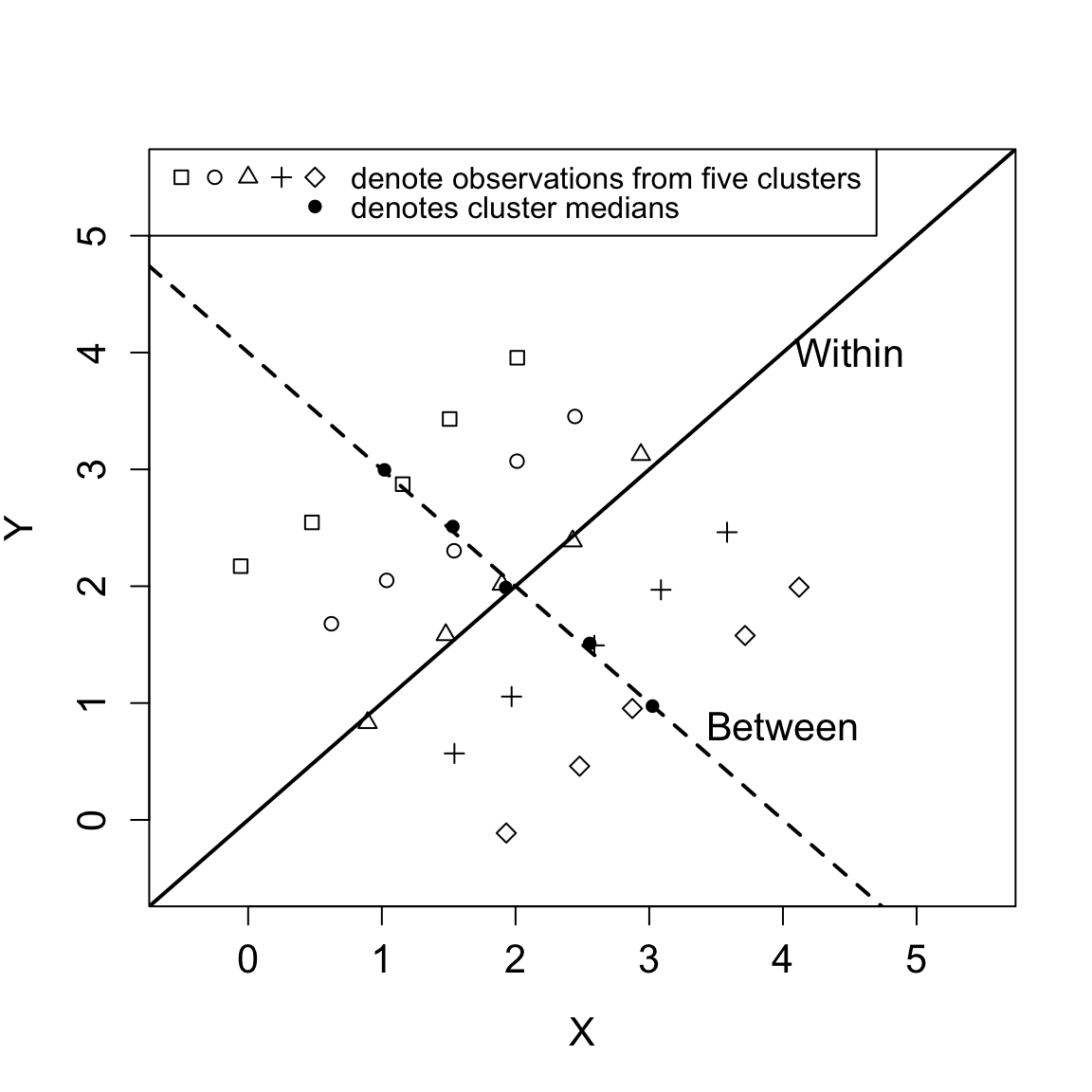
(a) $(\gamma_{t},\gamma_{b},\gamma_{w},\gamma_{I_{X}},\gamma_{I_{Y}})=(0,-1,1,0.5,0.5)$

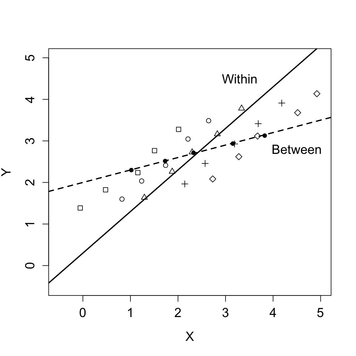
(b) $(\gamma_{t},\gamma_{b},\gamma_{w},\gamma_{I_{X}},\gamma_{I_{Y}})=(0.84,1,1,0.6,0.1)$

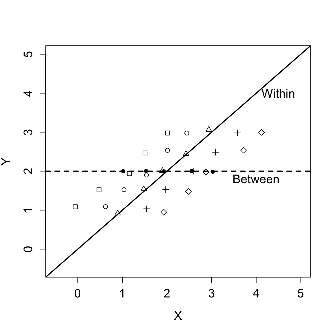
(c) $(\gamma_{t},\gamma_{b},\gamma_{w},\gamma_{I_{X}},\gamma_{I_{Y}})=(0.71,0,1,0.5,0)$

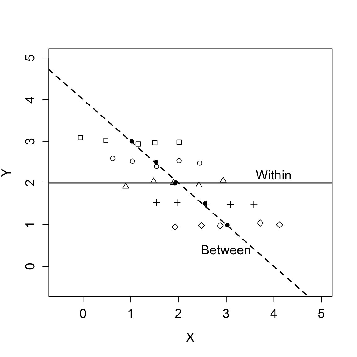
(d) $(\gamma_{t},\gamma_{b},\gamma_{w},\gamma_{I_{X}},\gamma_{I_{Y}})=(-0.71,-1,0,0.5,1)$

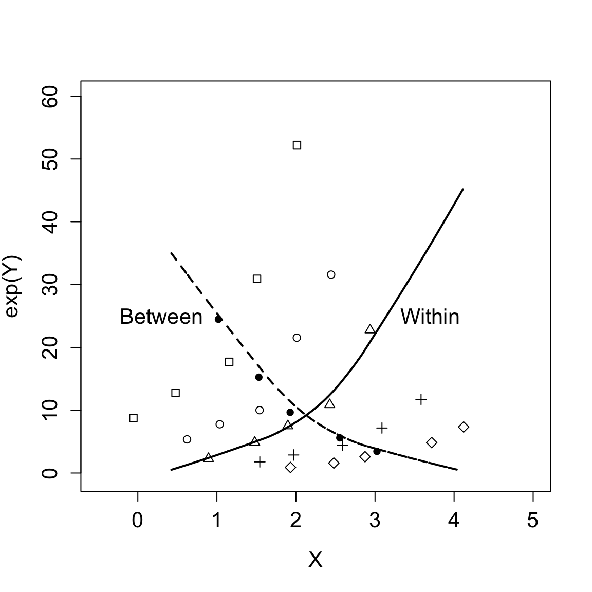
(e) $(\gamma_{t},\gamma_{b},\gamma_{w},\gamma_{I_{X}},\gamma_{I_{Y}})=(0,-1,1,0.5,0.5)$

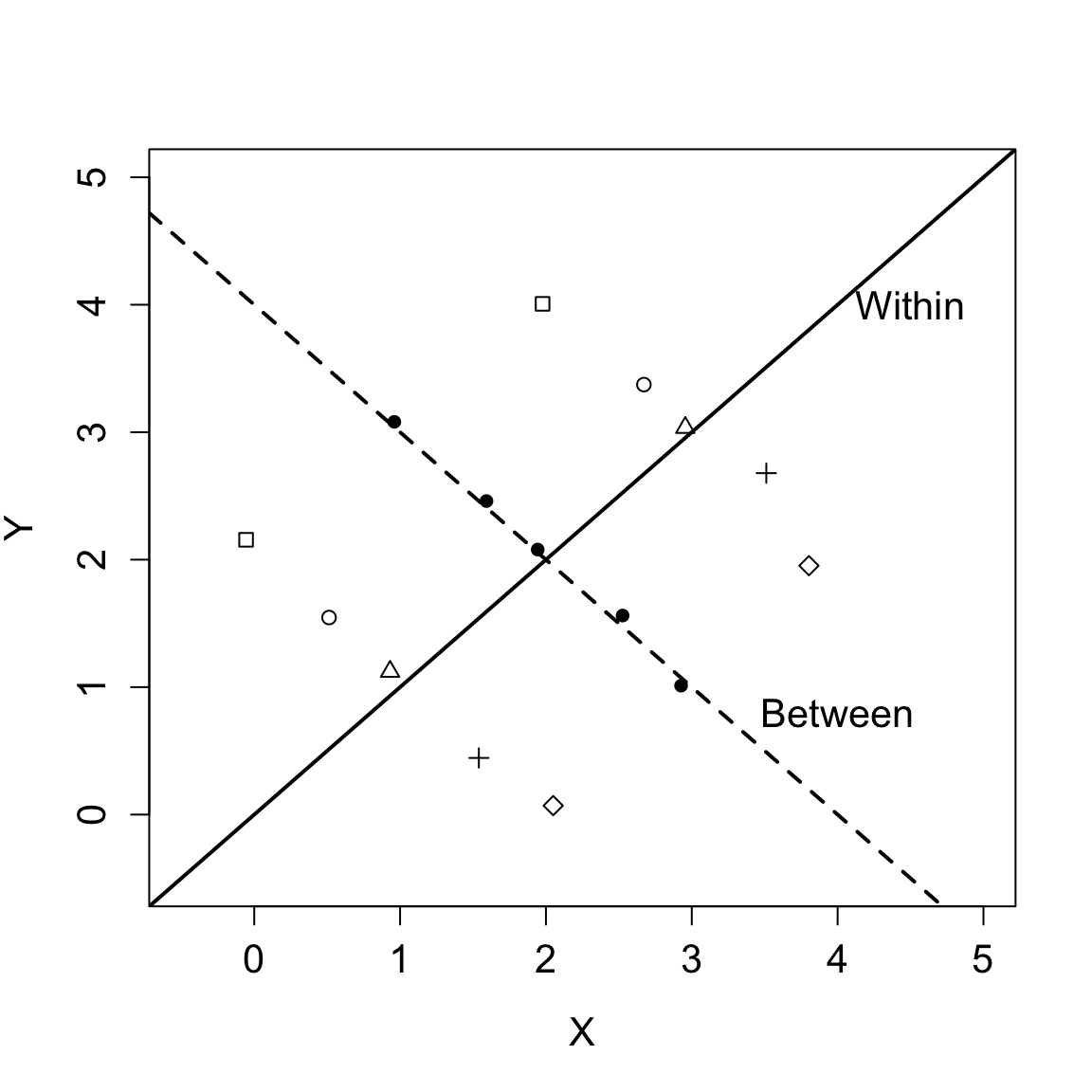
(f) $(\gamma_{t},\gamma_{b},\gamma_{w},\gamma_{I_{X}},\gamma_{I_{Y}})=(0,-1,1,-1,-1)$

Figure 1: Toy examples for the relationship between total ($\gamma_{t}$), between-cluster ($\gamma_{b}$), within-cluster ($\gamma_{w}$) Spearman rank correlations and the rank intraclass correlations ($\gamma_{I_{X}}$, $\gamma_{I_{Y}}$). For illustration purposes, we show five clusters and five (two for (f)) observations to represent the distribution of each cluster. Black dots represent cluster medians, and the other symbols represent the five clusters. The solid lines show the direction of the within-cluster correlation and the dashed lines show the direction of the between-cluster correlation.

We provide some toy examples to illustrate the relationship between $\gamma_{t}$, $\gamma_{b}$, and $\gamma_{w}$ under different rank ICCs of $X$ and $Y$ (Figure 1). Figures 1(a) and 1(b) show examples where $\gamma_{b}$ and $\gamma_{w}$ are in the opposite or same directions, respectively. If $X$ and $Y$ have moderate rank ICCs of 0.5, then $\gamma_{b}$ and $\gamma_{w}$ contribute equally to $\gamma_{t}$, and $\gamma_{t}$ is the average of $\gamma_{b}$ and $\gamma_{w}$ (Figure 1(a) and 1(e)). If the rank ICCs are large, $\gamma_{t}$ is dominated by $\gamma_{b}$, while if the rank ICCs are low, $\gamma_{t}$ is dominated by $\gamma_{w}$. More extremely, if one of the rank ICCs is close to 1, $\gamma_{t}$ is close to $\gamma_{b}\sqrt{\gamma_{I_{X}}\gamma_{I_{Y}}}$ (Figure 1(d)). On the contrary, if one of the rank ICCs is near 0, which means that the observations in a cluster are nearly independent, then $\gamma_{t}$ is close to $\gamma_{w}\sqrt{(1-\gamma_{I_{X}})(1-\gamma_{I_{Y}})}$ (Figure 1(c)). When cluster sizes in the population are finite, the rank ICCs can be negative. If any of the rank ICCs is negative, the relationship between $\gamma_{t}$, $\gamma_{b}$, and $\gamma_{w}$ is (6) rather than the simpler (7). Figure 1(f) illustrates an extreme example where the rank ICCs are both $-1$. (This happens when cluster sizes are two.) In this example, $\gamma_{b}$ and $\gamma_{w}$ are strong and opposite whereas the total correlation is zero.

5 Estimation

Since the total Spearman rank correlation is the Pearson correlation between $F^{*}_{X}$ and $F^{*}_{Y}$, our estimator of $\gamma_{t}$ is $\hat{\gamma}_{t}=corr(\hat{F}_{X}^{*},\hat{F}_{Y}^{*})$, which is a plug-in estimator. Given two-level data $\{(x_{ij},y_{ij}):i=1,2,...,n,j=1,2,...,k_{i}\}$ with a total number of observations of $N=\sum_{i=1}^{n}k_{i}$, a nonparametric estimator of the CDF of $X$ is $\hat{F}_{X}(x)=\sum_{i=1}^{n}\sum_{j=1}^{k_{i}}w_{ij}I(x_{ij}\leq x)$, where $w_{ij}$ is the weight of observation $x_{ij}$ and $\sum_{i=1}^{n}\sum_{j=1}^{k_{i}}w_{ij}=1$. The weight $w_{ij}$ depends on how we believe the data reflect the composition of the underlying hierarchical distribution; for example, $w_{ij}=1/(nk_{i})$ corresponds to equal weights for clusters and $w_{ij}=1/N$ corresponds to equal weights for observations (Tu et al., 2023). Similarly, we estimate $\hat{F}_{X}(x-)=\sum_{i=1}^{n}\sum_{j=1}^{k_{i}}w_{ij}I(x_{ij}<x)$, and define $\hat{F}^{*}_{X}(x)=\{\hat{F}_{X}(x)+\hat{F}_{X}(x-)\}/2$. Estimation is the same for $F^{*}_{Y}$. The general form of our estimator of $\gamma_{t}$ is

$$\hat{\gamma}_{t}=\frac{\sum\limits_{i=1}^{n}\sum\limits_{j=1}^{k_{i}}w_{ij}(\hat{F}^{*}_{X}(x_{ij})-\bar{\hat{F^{*}_{X}}})(\hat{F}^{*}_{Y}(y_{ij})-\bar{\hat{F^{*}_{Y}}})}{\sqrt{\sum\limits_{i=1}^{n}\sum\limits_{j=1}^{k_{i}}w_{ij}(\hat{F}^{*}_{X}(x_{ij})-\bar{\hat{F^{*}_{X}}})^{2}}\sqrt{\sum\limits_{i=1}^{n}\sum\limits_{j=1}^{k_{i}}w_{ij}(\hat{F}^{*}_{Y}(y_{ij})-\bar{\hat{F^{*}_{Y}}})^{2}}},$$

where $\bar{\hat{F^{*}_{X}}}=\sum\limits_{i=1}^{n}\sum\limits_{j=1}^{k_{i}}w_{ij}\hat{F}^{*}_{X}(x_{ij})$ and $\bar{\hat{F^{*}_{Y}}}=\sum\limits_{i=1}^{n}\sum\limits_{j=1}^{k_{i}}w_{ij}\hat{F}^{*}_{Y}(y_{ij})$. If we assign equal weights to clusters (i.e., $w_{ij}=1/(nk_{i})$), our estimator of the total Spearman rank correlation is equal to the estimator of Shih and Fay (2017).

Section 3 shows that $\gamma_{w}$ is identical to the covariate-adjusted partial Spearman rank correlation and can be expressed in terms of PSRs, suggesting that $\gamma_{w}$ can be estimated by sample PSRs (Liu et al., 2017). Hence, our estimator of $\gamma_{w}$ is

$$\hat{\gamma}_{w}=\frac{\sum\limits_{i=1}^{n}\sum\limits_{j=1}^{k_{i}}w_{ij}(x_{ij,res}-\bar{x}_{res})(y_{ij,res}-\bar{y}_{res})}{\sqrt{\sum\limits_{i=1}^{n}\sum\limits_{j=1}^{k_{i}}w_{ij}(x_{ij,res}-\bar{x}_{res})^{2}}\sqrt{\sum\limits_{i=1}^{n}\sum\limits_{j=1}^{k_{i}}w_{ij}(y_{ij,res}-\bar{y}_{res})^{2}}},$$ (8)

where $x_{ij,res}=r(x_{ij},\hat{F}_{X|i})$, $y_{ij,res}=r(y_{ij},\hat{F}_{Y|i})$, $\bar{x}_{res}=\sum\limits_{i=1}^{n}\sum\limits_{j=1}^{k_{i}}w_{ij}x_{ij,res}$, $\bar{y}_{res}=\sum\limits_{i=1}^{n}\sum\limits_{j=1}^{k_{i}}w_{ij}y_{ij,res}$. We can obtain PSRs using nonparametric, parametric, or semiparametric models. A nonparametric estimator of $F_{X|i}$ is simply the empirical CDF of $X$ in cluster $i$. Estimators from nonparametric models are the most robust but can be inefficient and unstable if cluster sizes are small. Parametric models are the most efficient under correct assumptions but less robust to extreme values, sensitive to model misspecification or outcome transformation, and not congruent with the spirit of Spearman rank correlation. To achieve a compromise between robustness and efficiency, we employ semiparametric models in which only the order information of outcomes is used and the clusters share a common latent variable distribution except for cluster-specific shifts. This way we can borrow information across clusters and still maintain the rank-based nature of Spearman rank correlation.

Specifically, we designate cluster 1 as the reference cluster, and define $Z_{i}$ ($i=2,\ldots,n$) as an indicator variable such that $Z_{i}=1$ when the observation is in cluster $i$ and $Z_{i}=0$ otherwise. We then model $X$ and $Y$ on $Z=(Z_{2},\ldots,Z_{n})^{T}$ to obtain PSRs for $X$ and $Y$, respectively. Here we incorporate the semiparametric linear transformation model where the monotonic transformation, $H_{X}(\cdot)$, is unspecified, $F_{X|Z}(x)=P\{H_{X}(\beta_{X}^{T}Z+\epsilon)\leq x|Z\}=F_{\epsilon}\{H_{X}^{-1}(x)-\beta_{X}^{T}Z\}$, where $\epsilon$ follows a known distribution and $\beta_{X}=(\beta_{X2},\ldots,\beta_{Xn})^{T}$. The semiparametric transformation model can be written in the form of the ordinal cumulative probability model (CPM), $g_{X}\{F_{X|Z}(x)\}=\alpha_{X}(x)-\beta_{X}^{T}Z$, where $\alpha_{X}(x)=H_{X}^{-1}(x)$ is estimated with a step function, and $g_{X}(\cdot)=F^{-1}_{\epsilon}$ is a link function (Liu et al., 2017). A similar model is fit for $Y$ on $Z$. Model estimation can be implemented using software for fitting ordinal cumulative probability (“link”) models with each unique outcome representing a separate ordinal category. For example, the orm() function in the rms package of R can be used (Harrell, 2015). After obtaining PSRs from the CPMs of $X$ on $Z$ and of $Y$ on $Z$, we then simply estimate $\gamma_{w}$ as in (8).

As mentioned in Section 3, we often use the cluster median as the cluster centroid, so $\gamma_{b}$ is Spearman rank correlation between cluster medians. One simple estimation approach is to estimate $\gamma_{b}$ as Spearman rank correlation between the sample cluster medians (i.e., $\{(\hat{\tilde{x_{i}}},\hat{\tilde{y_{i}}}):i=1,2,...,n\}$, where $\hat{\tilde{x_{i}}}$ and $\hat{\tilde{y_{i}}}$ are the medians of $\{x_{i1},...,x_{ik_{i}}\}$ and $\{y_{i1},...,y_{ik_{i}}\}$, respectively). However, this approach only uses information within clusters, which can have high variations with small cluster sizes. Thus, we consider estimating the cluster medians using CPMs of $X$ on $Z$ and of $Y$ on $Z$. The CPMs borrow information across clusters and their estimates of cluster medians are less variable than the simple estimates. Moreover, for ordered categorical data, the CPMs allow us to obtain cluster medians on the latent variable scale, thus simplifying the estimation of $\gamma_{b}$ by eliminating the need to consider all possible combinations of cluster medians on the original scale in the presence of clusters with two medians.

Let us consider a CPM of $X$ on $Z$, $g_{X}\{F_{X|Z}(x)\}=\alpha_{X}(x)-\beta_{X}^{T}Z$, where $g_{X}$ is a symmetric link function such as logit or probit. For any $Z=z$, let $x_{z}$ be the true median of $X$ given $Z=z$. Since $F_{X|Z=z}(x_{z})=0.5$ and $g_{X}(0.5)=0$, we have $0=\alpha_{X}(x_{z})-\beta_{X}^{T}z$ and $\alpha_{X}(x_{z})=\beta_{X}^{T}z$. That is, the monotone function $\alpha_{X}$ transforms the median $x_{z}$ to $\beta_{X}^{T}z$. In the setting of clustered data, $Z=(Z_{2},\ldots,Z_{n})^{T}$ is a vector of indicator variables for the clusters, and thus the cluster medians are 0 for cluster 1 and $\beta_{Xi}$ for cluster $i$ ($i=2,\ldots,n$). Since $\alpha_{X}$ is a monotonic increasing transformation, a Spearman rank correlation that involves the cluster medians of $X$ can be computed with $(0,\beta_{X2},\ldots,\beta_{Xn})^{T}$. Similarly, a Spearman rank correlation that involves the cluster medians of $Y$ can be computed with $(0,\beta_{Y2},\ldots,\beta_{Yn})^{T}$. All these values can be estimated from the CPMs. Thus, our estimator of $\gamma_{b}$ is the rank correlation over the $n$ pairs of estimated cluster medians, $\{(0,0),(\hat{\beta}_{X2},\hat{\beta}_{Y2}),\ldots,(\hat{\beta}_{Xn},\hat{\beta}_{Yn})\}$. Furthermore, we also consider weighting clusters in the estimation procedures for $\gamma_{b}$. Let $w_{i\cdot}$ denote the weight of cluster $i$ and $w_{i\cdot}=\sum_{j=1}^{k_{i}}w_{ij}$. A nonparametric estimator of the CDF of $\beta_{X}$ is $\hat{F}_{\beta_{X}}(t)=\sum_{i=1}^{n}w_{i\cdot}I(\hat{\beta}_{Xi}\leq t)$, similarly $\hat{F}_{\beta_{X}}(t-)=\sum_{i=1}^{n}w_{i\cdot}I(\hat{\beta}_{Xi}<t)$, and we define $\hat{F}_{\beta_{X}}^{*}(t)=\{\hat{F}_{\beta_{X}}(t)+\hat{F}_{\beta_{X}}(t-)\}/2$. Estimation for $F_{\beta_{Y}}^{*}$ is similar. Therefore, one estimator of $\gamma_{b}$ is

$$\hat{\gamma}_{b_{M}}=\frac{\sum\limits_{i=1}^{n}w_{i\cdot}(\hat{F}^{*}_{\beta_{X}}(\hat{\beta}_{Xi})-\bar{\hat{F}}^{*}_{\beta_{X}})(\hat{F}^{*}_{\beta_{Y}}(\hat{\beta}_{Yi})-\bar{\hat{F}}^{*}_{\beta_{Y}})}{\sqrt{\sum\limits_{i=1}^{n}w_{i\cdot}(\hat{F}^{*}_{\beta_{X}}(\hat{\beta}_{Xi})-\bar{\hat{F}}^{*}_{\beta_{X}})^{2}}\sqrt{\sum\limits_{i=1}^{n}w_{i\cdot}(\hat{F}^{*}_{\beta_{Y}}(\hat{\beta}_{Yi})-\bar{\hat{F}}^{*}_{\beta_{Y}})^{2}}},$$

where $\hat{\beta}_{X1}=\hat{\beta}_{Y1}=0$, $\bar{\hat{F}}^{*}_{\beta_{X}}=\sum\limits_{i=1}^{n}w_{i\cdot}\hat{F}^{*}_{\beta_{X}}(\hat{\beta}_{Xi})$, and $\bar{\hat{F}}^{*}_{\beta_{Y}}=\sum\limits_{i=1}^{n}w_{i\cdot}\hat{F}^{*}_{\beta_{Y}}(\hat{\beta}_{Yi})$. When $w_{i\cdot}=1/n$, $\bar{\hat{F}}^{*}_{\beta_{X}}=\bar{\hat{F}}^{*}_{\beta_{Y}}=1/2$.

If cluster sizes are very small, the estimates of $\beta_{X}$ and $\beta_{Y}$, and thus $\hat{\gamma}_{b_{M}}$, may be poor. We consider another estimation approach. As shown in Section 4 equation (6), $\gamma_{t}$ is approximated by a weighted sum of $\gamma_{w}$ and $\gamma_{b}$, where the weights are functions of $\gamma_{Ix}$ and $\gamma_{Iy}$. We can use this relationship to obtain an estimate of $\gamma_{b}$,

$$\hat{\gamma}_{b_{A}}=\frac{\hat{\gamma}_{t}-\sqrt{(1-\hat{\gamma}_{I_{X}}+\hat{D}_{X})(1-\hat{\gamma}_{I_{Y}}+\hat{D}_{Y})}\hat{\gamma}_{w}}{\sqrt{(\hat{\gamma}_{I_{X}}-\hat{D}_{X})(\hat{\gamma}_{I_{Y}}-\hat{D}_{Y})}},$$

where $\hat{\gamma}_{I_{X}}$ and $\hat{\gamma}_{I_{Y}}$ are nonparametric estimators of $\gamma_{I_{X}}$ and $\gamma_{I_{X}}$ (Tu et al., 2023), $\hat{D}_{X}=\\ \frac{\sum_{i=1}^{n}w_{i\cdot}\sum_{j<j^{\prime}}\frac{2}{k_{i}(k_{i}-1)}[\hat{F}^{*}(x_{ij})-\bar{F}^{*}_{i}][\hat{F}^{*}(x_{ij^{\prime}})-\bar{F}^{*}_{i}]}{\sum_{i=1}^{n}\sum_{j=1}^{k_{i}}w_{ij}[\hat{F}^{*}(x_{ij})-\bar{F}^{*}]^{2}}$, $\bar{F}^{*}_{i}=\sum_{j}F^{*}(x_{ij})/k_{i}$, and similar for $\hat{D}_{Y}$. If the cluster size in the population is infinite, $D_{X}=D_{Y}=0$, then $\hat{\gamma}_{b_{A}}=\frac{\hat{\gamma}_{t}-\sqrt{(1-\hat{\gamma}_{Ix})(1-\hat{\gamma}_{Iy})}\hat{\gamma}_{w}}{\sqrt{\hat{\gamma}_{Ix}\hat{\gamma}_{Iy}}}$. Note that $\hat{\gamma}_{b_{A}}$ can be greater than 1 or less than $-1$; in those cases, we define $\hat{\gamma}_{b_{A}}$ to be $1$ or $-1$, respectively. When cluster sizes are very small, $\hat{\gamma}_{b_{A}}$ may be preferable over $\hat{\gamma}_{b_{M}}$. If either of the rank ICCs is very small, $\sqrt{\hat{\gamma}_{Ix}\hat{\gamma}_{Iy}}\approx 0$ and $\hat{\gamma}_{b_{A}}$ can be unstable.

6 Inference

The large sample distribution of $\hat{\gamma}_{w}$ can be obtained by bootstrapping or large sample approximation. Here we focus on the large sample approach using M-estimation (Stefanski and Boos, 2002). The CPM is fit by minimizing the multinomial/nonparametric likelihood, and then the variance of parameter estimates can be estimated using a sandwich variance estimator that accounts for clustering. This is equivalent to fitting generalized estimating equation (GEE) methods for ordinal response variables with independence working correlation (Tian et al., 2023). Let $\psi_{X}(\cdot)=\mathbf{U}_{X}(\boldsymbol{\theta})$ denote the estimating function for the CPM of $X$ on $Z$ with a vector of parameters $\boldsymbol{\theta}_{X}$, and $\psi_{Y}(\cdot)=\mathbf{U}_{Y}(\boldsymbol{\theta})$ denote the estimating function for the CPM of $Y$ on $Z$ with a vector of parameters $\boldsymbol{\theta}_{Y}$. See the Supplementary Materials for details about these estimating functions. The components necessary for computing $\gamma_{w}$ are denoted by $\theta_{w1}$, $\theta_{w2}$, $\theta_{w3}$, $\theta_{w4}$, and $\theta_{w5}$ such that $\gamma_{w}=(\theta_{w3}-\theta_{w1}\theta_{w2})/\sqrt{(\theta_{w4}-\theta_{w1}^{2})(\theta_{w5}-\theta_{w2}^{2})}$, where $\theta_{w1}=E(X_{ij,res})$, $\theta_{w2}=E(Y_{ij,res})$, $\theta_{w3}=E(X_{ij,res}Y_{ij,res})$, $\theta_{w4}=E(X_{ij,res}^{2})$, $\theta_{w5}=E(Y_{ij,res}^{2})$. We can stack $\psi_{X}(\cdot)$ and $\psi_{Y}(\cdot)$ together with these components and then have the following estimating function,

$$\psi_{w}(\mathbf{X}_{i},\mathbf{Y}_{i},\mathbf{Z}_{i},\boldsymbol{\theta}_{w})$$

$$=\{\psi_{X}(\mathbf{X}_{i},\mathbf{Z}_{i},\boldsymbol{\theta}_{X}),\psi_{Y}(\mathbf{Y}_{i},\mathbf{Z}_{i},\boldsymbol{\theta}_{Y}),I_{i}^{T}\mathbf{X}_{i,res}/k_{i}-\theta_{w1},I_{i}^{T}\mathbf{Y}_{i,res}/k_{i}-\theta_{w2},$$

$$\mathbf{X}_{i,res}^{T}\mathbf{Y}_{i,res}/k_{i}-\theta_{w3},\mathbf{X}_{i,res}^{T}\mathbf{X}_{i,res}/k_{i}-\theta_{w4},\mathbf{Y}_{i,res}^{T}\mathbf{Y}_{i,res}/k_{i}-\theta_{w5}\}^{T},$$

where $\boldsymbol{\theta}_{w}=(\boldsymbol{\theta}_{X},\boldsymbol{\theta}_{Y},\theta_{w1},\theta_{w2},\theta_{w3},\theta_{w4},\theta_{w5})$, $I_{i}$ is a vector of ones with a length of $k_{i}$. The estimating equations are $\sum_{i=1}^{n}\psi_{w}(\mathbf{X}_{i},\mathbf{Y}_{i},\mathbf{Z}_{i};\hat{\boldsymbol{\theta}}_{w})=0$. Under standard regularity conditions (Stefanski and Boos, 2002), then we have $\sqrt{n}(\hat{\boldsymbol{\theta}}_{w}-\boldsymbol{\theta}_{w})\stackrel{{\scriptstyle d}}{{\rightarrow}}MVN(\mathbf{0},\mathbf{V}(\boldsymbol{\theta}_{w}))$, where $\mathbf{V}(\boldsymbol{\theta}_{w})=\mathbf{A}(\boldsymbol{\theta}_{w})^{-1}\mathbf{B}(\boldsymbol{\theta}_{w})\{\mathbf{A}(\boldsymbol{\theta}_{w})^{-1}\}^{T}$, $\mathbf{A}(\boldsymbol{\theta}_{w})=E[-\partial\psi_{w}(\mathbf{X}_{i},\mathbf{Y}_{i},\mathbf{Z}_{i},\boldsymbol{\theta}_{w})/\partial\boldsymbol{\theta}_{w}^{T}]$,
and $\mathbf{B}(\boldsymbol{\theta}_{w})=E[\psi_{w}(\mathbf{X}_{i},\mathbf{Y}_{i},\mathbf{Z}_{i},\boldsymbol{\theta}_{w})\psi_{w}(\mathbf{X}_{i},\mathbf{Y}_{i},\mathbf{Z}_{i},\boldsymbol{\theta}_{w})^{T}]$. Since our estimator of $\gamma_{w}$ is a function of $\hat{\theta}_{w1}$, $\hat{\theta}_{w2}$, $\hat{\theta}_{w3}$, $\hat{\theta}_{w4}$, and $\hat{\theta}_{w5}$, the delta method can be used to obtain its large sample distribution. Then we can compute the asymptotic standard error (SE) of $\gamma_{w}$ and construct confidence intervals (CIs) for $\gamma_{w}$.

We use a similar approach to obtain the large sample distribution of $\hat{\gamma}_{b_{M}}$. Let $\boldsymbol{\beta}_{X}=(0,\beta_{X2},...,\beta_{Xn})^{T}$ and $\boldsymbol{\beta}_{Y}=(0,\beta_{Y2},...,\beta_{Yn})^{T}$ denote the coefficients of cluster index in the CPMs of $X$ and $Y$, respectively. Note that the coefficient of the reference cluster is zero. To obtain the asymptotic variance of $\gamma_{b}$, we treat $\boldsymbol{\beta}_{X}$ and $\boldsymbol{\beta}_{Y}$ as random effects, for simplicity assuming that $\beta_{Xi}\stackrel{{\scriptstyle i.i.d}}{{\sim}}N(\mu_{\beta_{X}},\sigma^{2}_{\beta_{X}})$ and $\beta_{Yi}\stackrel{{\scriptstyle i.i.d}}{{\sim}}N(\mu_{\beta_{Y}},\sigma^{2}_{\beta_{Y}})$. The components necessary for computing $\gamma_{b}$ are denoted by $\theta_{b1}$, $\theta_{b2}$, $\theta_{b3}$, $\theta_{b4}$, and $\theta_{b5}$ such that $\gamma_{b}=(\theta_{b3}-\theta_{b1}\theta_{b2})/\sqrt{(\theta_{b4}-\theta_{b1}^{2})(\theta_{b5}-\theta_{b2}^{2})}$, where $\theta_{b1}=E[F_{\beta_{X}}(\beta_{Xi})]$, $\theta_{b2}=E[F_{\beta_{Y}}(\beta_{Yi})]$,
$\theta_{b3}=E[F_{\beta_{X}}(\beta_{Xi})F_{\beta_{Y}}(\beta_{Yi})]$, $\theta_{b4}=E\{[F_{\beta_{X}}(\beta_{Xi})]^{2}\}$, $\theta_{b5}=E\{[F_{\beta_{Y}}^{2}(\beta_{Yi})]^{2}\}$, and $F_{\beta_{X}}$ and $F_{\beta_{Y}}$ are the CDFs of normal distributions. Note that $E[F_{\beta_{X}}(\beta_{Xi})]=E[F_{\beta_{X}}(\beta_{Yi})]=1/2$ in theory but they may not be $1/2$ in estimation if $w_{i\cdot}\neq 1/n$. Similar to the inference procedure of $\gamma_{w}$ above, we stack $\psi_{X}(\cdot)$ and $\psi_{Y}(\cdot)$ with the components needed to compute $\gamma_{b}$ stacked together, yielding the following estimating function,

$$\psi_{b}(\mathbf{X}_{i},\mathbf{Y}_{i},\mathbf{Z}_{i},\boldsymbol{\theta}_{b})$$

$$=\{\psi_{X}(\mathbf{X}_{i},\mathbf{Z}_{i},\boldsymbol{\theta}_{X}),\psi_{Y}(\mathbf{Y}_{i},\mathbf{Z}_{i},\boldsymbol{\theta}_{Y}),\beta_{Xi}-\mu_{\beta_{X}},\beta_{Yi}-\mu_{\beta_{Y}},\beta_{Xi}^{2}-M_{\beta_{X}},\beta_{Yi}^{2}-M_{\beta_{Y}},$$

$$F_{\beta_{X}}(\beta_{Xi})-\theta_{b1},F_{\beta_{Y}}(\beta_{Yi})-\theta_{b2},F_{\beta_{X}}(\beta_{Xi})F_{\beta_{Y}}(\beta_{Yi})-\theta_{b3},[F_{\beta_{X}}(\beta_{Xi})]^{2}-\theta_{b4},[F_{\beta_{X}}(\beta_{Yi})]^{2}-\theta_{b5}\}^{T},$$

where $\boldsymbol{\theta}_{b}=(\boldsymbol{\theta}_{X},\boldsymbol{\theta}_{Y},\mu_{\beta_{X}},\mu_{\beta_{Y}},M_{\beta_{X}},M_{\beta_{Y}},\theta_{b1},\theta_{b2},\theta_{b3},\theta_{b4},\theta_{b5})$, $M_{\beta_{X}}=E(\beta_{X}^{2})=\mu_{\beta_{X}}^{2}+\sigma^{2}_{\beta_{X}}$, and $M_{\beta_{Y}}=E(\beta_{Y}^{2})=\mu_{\beta_{Y}}^{2}+\sigma^{2}_{\beta_{Y}}$. The estimating equations are $\sum_{i=1}^{n}\psi_{b}(\mathbf{X}_{i},\mathbf{Y}_{i},\mathbf{Z}_{i};\hat{\boldsymbol{\theta}}_{b})=0$. We have $\sqrt{n}(\hat{\boldsymbol{\theta}}_{b}-\boldsymbol{\theta}_{b})\stackrel{{\scriptstyle d}}{{\rightarrow}}MVN(\mathbf{0},\mathbf{V}(\boldsymbol{\theta}_{b}))$ under standard regularity conditions (Stefanski and Boos, 2002), where $\mathbf{V}(\boldsymbol{\theta}_{b})=\mathbf{A}(\boldsymbol{\theta}_{b})^{-1}\mathbf{B}(\boldsymbol{\theta}_{b})\{\mathbf{A}(\boldsymbol{\theta}_{b})^{-1}\}^{T}$, $\mathbf{A}(\boldsymbol{\theta}_{b})=E[-\partial\psi_{b}(\mathbf{X}_{i},\mathbf{Y}_{i},\mathbf{Z}_{i},\boldsymbol{\theta})/\partial\boldsymbol{\theta}^{T}_{b}]$, and $\mathbf{B}(\boldsymbol{\theta})=E[\psi_{b}(\mathbf{X}_{i},\mathbf{Y}_{i},\mathbf{Z}_{i},\boldsymbol{\theta}_{b})\psi_{b}(\mathbf{X}_{i},\mathbf{Y}_{i},\mathbf{Z}_{i},\boldsymbol{\theta}_{b})^{T}]$. The large sample distribution of $\hat{\gamma}_{b_{M}}$ can be derived from the large sample distribution of $\hat{\boldsymbol{\theta}}_{b}$ using the delta method. We also use this expression for inference for $\hat{\gamma}_{b_{A}}$.

As mentioned in Section 5, if the same weight is assigned to all the observations, our estimator of the total Spearman rank correlation $\hat{\gamma}_{t}$ equals the estimator of Shih and Fay (2017). Hence, we adapt the inference method of Shih and Fay (2017) via incorporating weighting into the estimation procedures to obtain the asymptotic variance of $\hat{\gamma}_{t}$. Shih and Fay (2017) have provided an analytical form for the asymptotic distribution of the estimator of $\gamma_{t}$, which is a function of $X_{ij}$, $Y_{ij}$, $F_{X}$, $F_{Y}$, and $F_{XY}$. The asymptotic variance can be estimated with $\hat{F}_{X}$, $\hat{F}_{Y}$, and $\hat{F}_{XY}$ plugged in for $F_{X}$, $F_{Y}$, and $F_{XY}$. Here we allow $\hat{F}_{X}$, $\hat{F}_{Y}$, and $\hat{F}_{XY}$ to be obtained based on either assigning equal weights to observations or assigning equal weights to clusters, and then plug them in to estimate the asymptotic variance of $\hat{\gamma}_{t}$.

7 Simulations

We used a bivariate additive model for data generation: $\begin{pmatrix}X_{0ij}\\ Y_{0ij}\end{pmatrix}=\begin{pmatrix}U_{Xi}\\ U_{Yi}\end{pmatrix}+\begin{pmatrix}R_{Xij}\\ R_{Yij}\end{pmatrix},$ where $\begin{pmatrix}U_{Xi}\\ U_{Yi}\end{pmatrix}\stackrel{{\scriptstyle i.i.d}}{{\sim}}N\begin{pmatrix}\begin{pmatrix}1\\ -1\end{pmatrix},\begin{pmatrix}1&\rho_{0b}\\ \rho_{0b}&1\end{pmatrix}\end{pmatrix}$, $\begin{pmatrix}R_{Xij}\\ R_{Yij}\end{pmatrix}\stackrel{{\scriptstyle i.i.d}}{{\sim}}N\begin{pmatrix}\begin{pmatrix}0\\ 0\end{pmatrix},\begin{pmatrix}1&\rho_{0w}\\ \rho_{0w}&1\end{pmatrix}\end{pmatrix}$. Here, $\rho_{0t}=(\rho_{0b}+\rho_{0w})/2$. Let $(X_{ij},Y_{ij})$ be the observation of the $j$th individual in the $i$th cluster, where $i=1,2,....,n$; $j=1,2,...,k_{i}$; and $k_{i}$ is the size of the $i$th cluster. We considered three scenarios: (I) $X_{ij}=X_{0ij}$ and $Y_{ij}=Y_{0ij}$; (II) $X_{ij}=X_{0ij}$ and $Y_{ij}=\exp(Y_{0ij})$; (III) $X_{ij}=\exp(U_{Xi})+R_{Xij}$ and $Y_{ij}=\exp(\exp(U_{Yi})+R_{Yij})$. Under Scenarios I and II, since $(X_{0ij},Y_{0ij})^{T}$ is bivariate normal, the true total, between-, and within-cluster Spearman rank correlations are $\gamma_{t}=6\arcsin(\rho_{0t}/2)/\pi$, $\gamma_{b}=6\arcsin(\rho_{0b}/2)/\pi$, and $\gamma_{w}=6\arcsin(\rho_{0w}/2)/\pi$ (Pearson, 1907). Under Scenario III, $\gamma_{b}$ and $\gamma_{w}$ are the same as those in Scenarios I and II, but $\gamma_{t}$ is different because $(X_{ij},Y_{ij})^{T}$ is not normally distributed. We empirically computed $\gamma_{t}$ under Scenario III by generating one million clusters each with 100 observations, and then computing $\gamma_{t}$. We also empirically computed the total, between- and within-cluster Pearson correlations (i.e., $\rho_{t}$, $\rho_{b}$, and $\rho_{w}$) under Scenarios II and III. While $\gamma_{b}$ and $\gamma_{w}$ are identical under the three scenarios, $\rho_{b}$ and $\rho_{w}$ are sensitive to skewness and depend on the scale of interest (Table 1).

We first evaluated the performance of our estimators of $\gamma_{b}$, $\gamma_{w}$, and $\gamma_{t}$ for continuous data. The simulations were conducted under Scenarios I, II, and III at $n=100$, and $(\rho_{0b},\rho_{0w})\in\{(0.8,0.7),(0.8,0),(0,0.8),(0,0),(0.8,-0.7)\}$. In Scenarios I and II, the rank ICCs of $X$ and $Y$ are both 0.48. In Scenario III, the rank ICC of $X$ is 0.97 while that of $Y$ is 0.37. We considered various configurations of cluster size under Scenarios I and II: $k_{i}=10$, $k_{i}=20$, $k_{i}=30$, and $k_{i}$ uniformly ranging from 1 to 50. We compared our estimators with naive nonparametric estimators: $\hat{\gamma}_{b_{n}}$ estimated by Spearman rank correlation between sample cluster medians and $\hat{\gamma}_{w_{n}}$ estimated by the rank correlation of within-cluster deviations (differences) from sample cluster medians. Furthermore, we compared the Spearman rank correlations with the Pearson correlations in Scenario I. The estimators of $\rho_{b}$ and $\rho_{w}$ are based on one-way random effects models: $\rho_{b}$ is estimated by Pearson correlation between the estimated cluster means from the random effects models and $\rho_{w}$ is estimated by Pearson correlation between the individual deviations from the estimated cluster means (Snijders and Bosker, 1999).

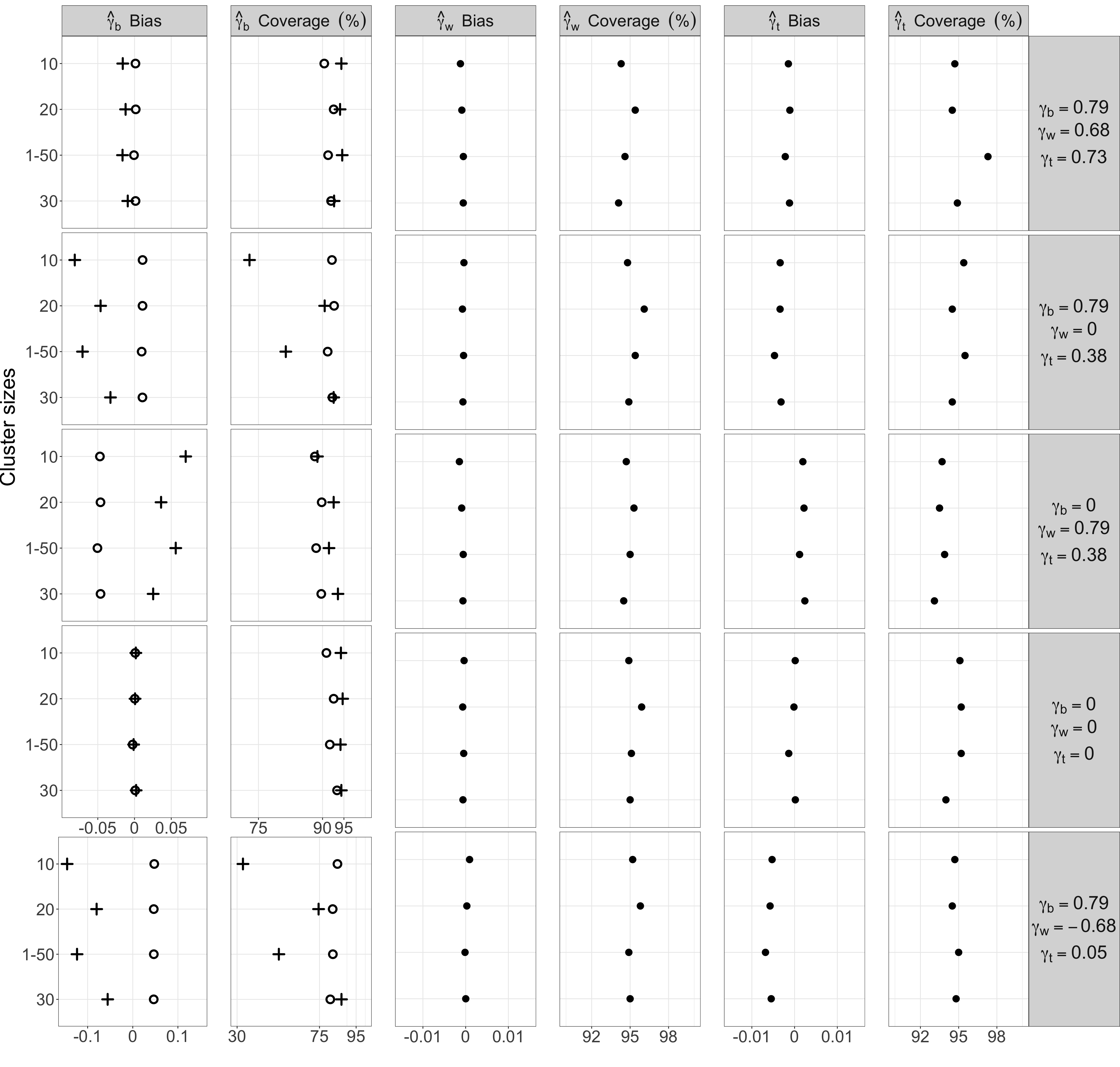
Figure 2: Bias and coverage of 95% confidence intervals for our estimators of $\gamma_{b}$, $\gamma_{w}$, and $\gamma_{t}$ at different true values and different cluster sizes under Scenarios I (normality) and II (exponentiated $Y$). The circle sign stands for the approximation-based estimator ($\hat{\gamma}_{b_{A}}$) of $\gamma_{b}$, and the plus sign stands for the cluster-median-based estimator ($\hat{\gamma}_{b_{M}}$) of $\gamma_{b}$. The number of clusters was set at 100. “1-50” means the cluster size follows a uniform distribution from 1 to 50.

In general, our estimators of $\gamma_{b}$, $\gamma_{w}$, and $\gamma_{t}$ had low bias and good coverage with modest numbers of clusters in Scenarios I and II (Figure 2). They were also robust to the skewed data in Scenario II and they had lower bias than $\hat{\gamma}_{b_{n}}$ and $\hat{\gamma}_{w_{n}}$ (Web Table 1). In the extreme case where $\gamma_{b}$ and $\gamma_{w}$ are both strong but opposite (i.e., last row of Figure 2), our estimators of $\gamma_{b}$ were biased. In the other settings where $\gamma_{b}$ and $\gamma_{w}$ greatly differed (i.e., rows 2-3 of Figure 2), the estimators of $\gamma_{b}$ were also biased, although to a lesser extent. In these settings, the bias of $\hat{\gamma}_{b_{A}}$ was relatively smaller than that of $\hat{\gamma}_{b_{M}}$, particularly with small cluster sizes. As the cluster size increased, the bias of $\hat{\gamma}_{b_{M}}$ decreased, whereas the bias of $\hat{\gamma}_{b_{A}}$ remained relatively stable (also seen in Web Table 2). It is worth noting that in the extreme case (last row of Figure 2), the estimator of the between-cluster Pearson correlation based on random effects models also had similar bias, even when the data were normally distributed (Web Table 3).

In Scenario III, our estimator of $\gamma_{w}$ still had low bias and good coverage (Web Table 4). In our setup, $E[U_{Yi}]=-1$, our estimators of $\gamma_{b}$ and $\gamma_{t}$ had more bias under Scenario III than under Scenarios I and II (Web Table 4a). This is because $U_{Yi}$ was exponentiated in Scenario III, which led to cluster means that had a much smaller variance than that of the within-cluster deviations. In this setting, the within-cluster deviation often dominated the value of $Y_{ij}$ creating data where it is difficult to see the effect of clustering over the within-cluster variance. Our estimator of $\gamma_{t}$ struggled in this setting, producing biased estimates of $\gamma_{t}$ and thus biased estimates of $\gamma_{b}$ based on the approximation (7). In addition, estimation of $\gamma_{b}$ using $\hat{\gamma}_{b_{M}}$ also was biased, as estimated cluster medians, even with fairly larger cluster sizes, often were far from their true rankings due to the large residual noise. When $E[U_{Yi}]$ was changed from -1 to 1, the cluster means had a larger variance than that of the within-cluster deviations, leading to much smaller bias in the estimates of $\gamma_{t}$ and $\gamma_{b}$ (Web Table 4b).

We then evaluated the performance of our estimators when the rank ICC was negative, which occurs when $k_{i}=2$. Our estimators of $\gamma_{t}$, $\gamma_{b}$, and $\gamma_{w}$ had very low bias and good coverage. Details are in the Supplementary Materials Web Table 5.

Furthermore, we investigated the performance of our estimators when the link function of the CPM was misspecified as logit, loglog, and cloglog under Scenario II. We conducted 1000 simulations at $n=100$ and $k_{i}=20$. Our estimators of $\gamma_{b}$, $\gamma_{w}$, and $\gamma_{t}$ performed similarly under the logit link as they did under the correct probit link function (Web Table 6). When the link function was misspecified as loglog or cloglog, if $\gamma_{w}$ was large and had the opposite direction of $\gamma_{b}$, our estimator of $\gamma_{w}$ had bias toward the direction of $\gamma_{b}$.

We also evaluated the performance of our estimators for ordered categorical data. We simulated 5-level and 10-level ordered categorical data by discretizing $X_{ij}$ and $Y_{ij}$ in Scenario I with cutoffs at quantiles (i.e., using the 0.2, 0.4, 0.6, 0.8 quantiles for 5 levels; and the 0.1, 0.2, …, 0.8, 0.9 quantiles for 10 levels). We empirically computed $\gamma_{t}$, $\gamma_{b}$, and $\gamma_{w}$ by generating one million clusters and 100 observations per cluster, with cluster medians analytically derived. The values of $\gamma_{t}$, $\gamma_{b}$, and $\gamma_{w}$ of the 10-level ordered categorical variables are close to those of the continuous variables, while those of the 5-level ordered categorical variables are slightly smaller (Web Table 7). We conducted 1000 simulations at $n=100$ and $k_{i}=20$. Our estimators of $\gamma_{b}$, $\gamma_{w}$, and $\gamma_{t}$ had very low bias and good coverage (Web Table 7). When $\gamma_{b}$ was large, $\hat{\gamma}_{b_{A}}$ had bias, which might be due to equation (7) being a poor approximation of $\gamma_{t}$ with ordered categorical data. This bias decreased as the number of ordered categories increased.

8 Applications

8.1 Longitudinal biomarker data

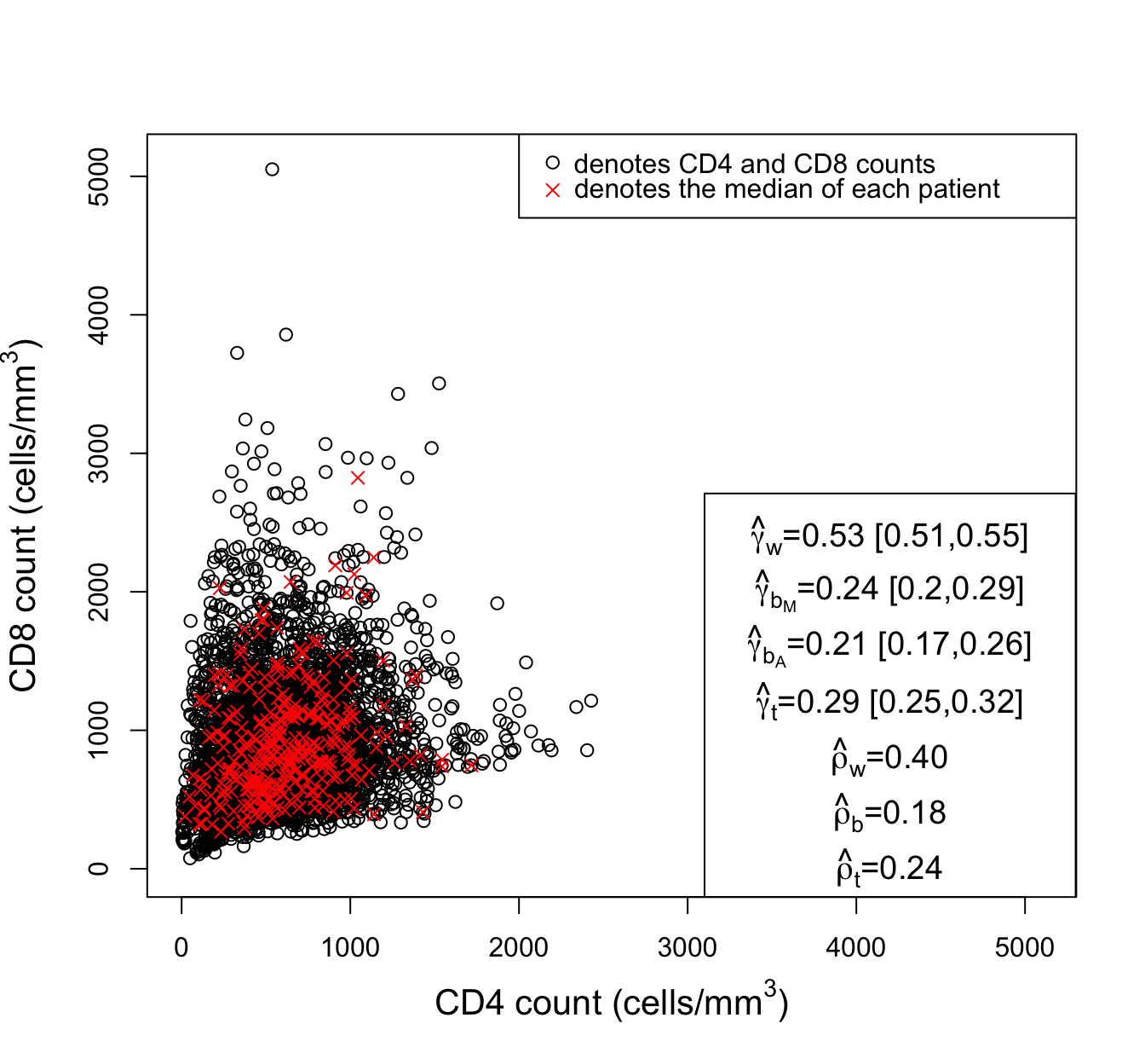
(a) Original scale

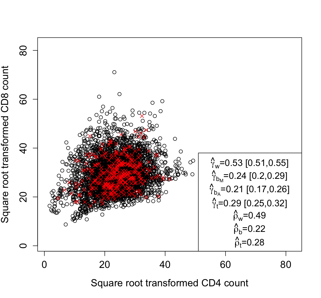
(b) Square-root transformation

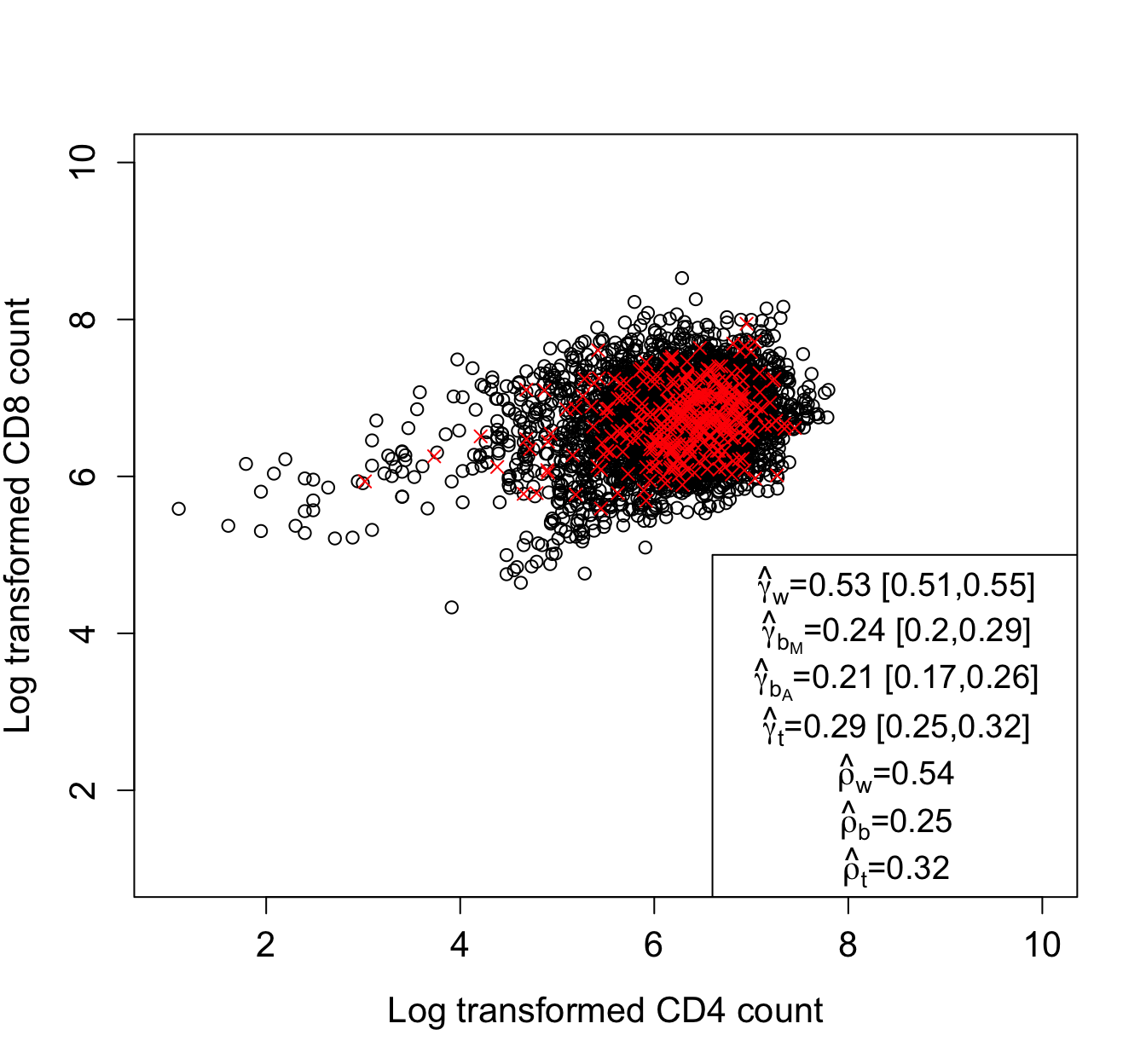
(c) Log transformation

Figure 3: Scatter plot of CD4 and CD8 counts (cells/mm³) and estimates of total, between-, and within-cluster Spearman rank ($\gamma_{t}$, $\gamma_{b}$, $\gamma_{w}$, [$95\%$ CIs]) and Pearson ($\rho_{t}$, $\rho_{b}$, $\rho_{w}$) correlations. The red cross sign represents the sample cluster median and the circle sign represents the observation. $\hat{\gamma}_{b_{M}}$ is the estimator of $\gamma_{b}$ based on cluster medians obtained from CPM and $\hat{\gamma}_{b_{A}}$ is the estimator of $\gamma_{b}$ based on the linear approximation.

Repeated measures of CD4 and CD8 lymphocyte counts (cells/mm³) were taken on 325 women living with HIV who started antiretroviral therapy (ART) at the Vanderbilt Comprehensive Care Clinic between 1998 and 2012 (Castilho et al., 2016). There is interest in evaluating the correlation between same-day CD4 and CD8 counts while considering the potential clustering in the data. All same-day CD4 and CD8 measurements taken within $\pm 4$ months of ART initiation were included in analyses; the number of observations per woman ranged from 1 to 54. In this case, the cluster is the person, so it makes sense to assign equal weights to people rather than measurements. The data were very skewed, especially the CD8 count (Figure 3).

The rank ICC estimates of CD4 and CD8 counts were 0.77 and 0.76, respectively, suggesting strong similarity between measurements from the same woman. The between-cluster Spearman rank correlation was estimated to be $\hat{\gamma}_{b_{M}}=0.24$ (95% CI: [0.20,0.29]) via cluster medians obtained from CPMs and was estimated to be $\hat{\gamma}_{b_{A}}=0.21$ (95% CI: [0.17,0.26]) via the approximation approach, indicating a weak but positive correlation between median CD4 and CD8 counts (Figure 3). The Spearman rank correlation between the sample cluster medians was 0.24, close to our between-cluster Spearman rank correlation estimates. The within-cluster Spearman rank correlation estimate was 0.53 (95%: [0.51,0.55]), suggesting moderate correlation between the fluctuations in the repeated CD4 and CD8 measurements. The total Spearman rank correlation estimate, 0.29 (95% CI: [0.25,0.32]), suggests a weak to moderate overall correlation after combining between-cluster and within-cluster correlations.

The between-cluster, within-cluster, and total Pearson correlation estimates on the original scale obtained from a random effects model were estimated to be 0.18, 0.40, and 0.24, respectively, which were impacted by some extreme measurements. The three Pearson correlations were estimated to be 0.22, 0.49, and 0.28, respectively, after square root transformation, and 0.25, 0.54, and 0.32, respectively, after log transformation. The notable differences in the three Pearson correlation estimates after data transformation demonstrate the sensitivity of Pearson correlation to the choice of scale. In contrast, our estimates of between-cluster, within-cluster, and total Spearman rank correlations are invariant to any monotonic transformation.

8.2 Cluster randomized controlled trial data

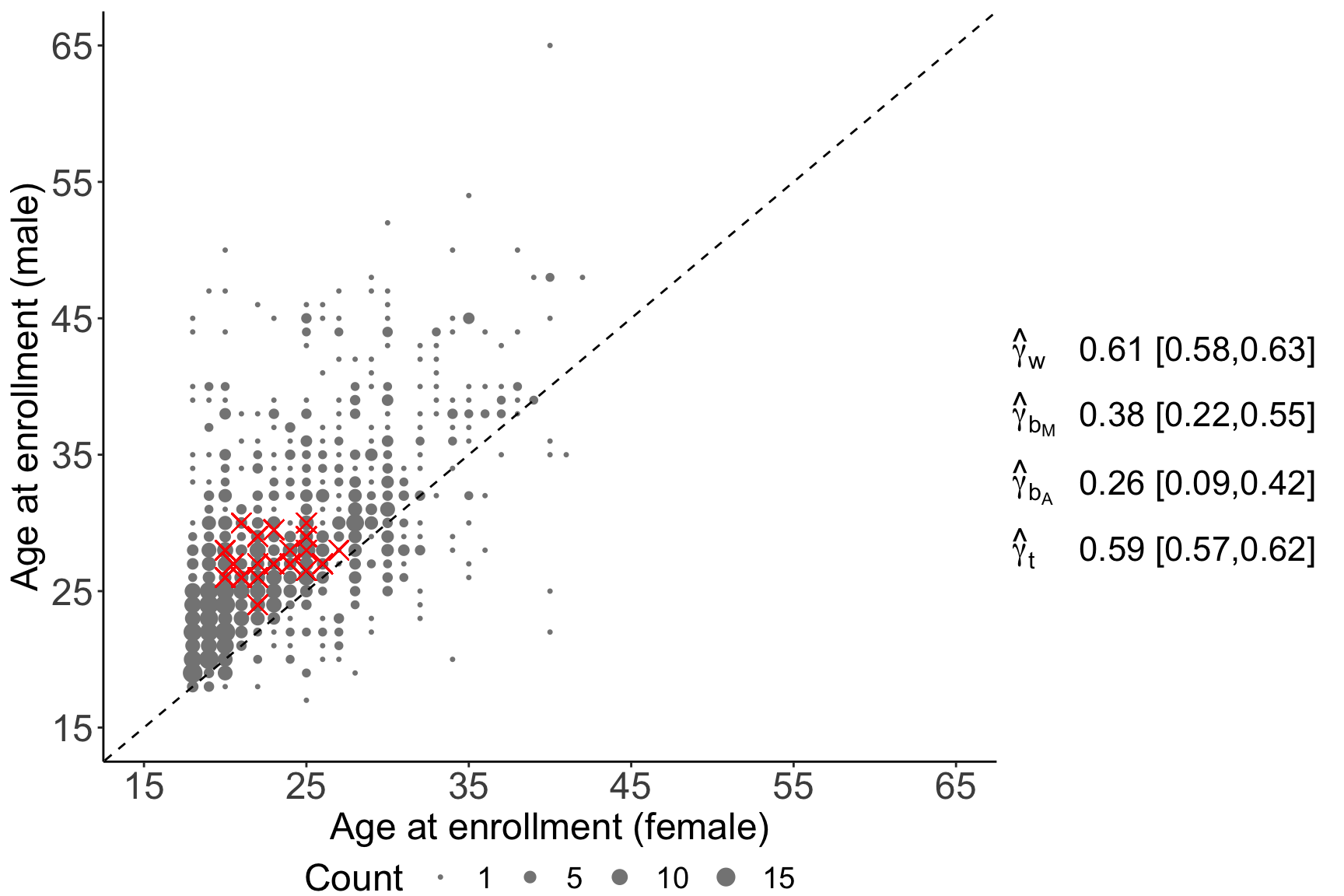
(a) Age at enrollment

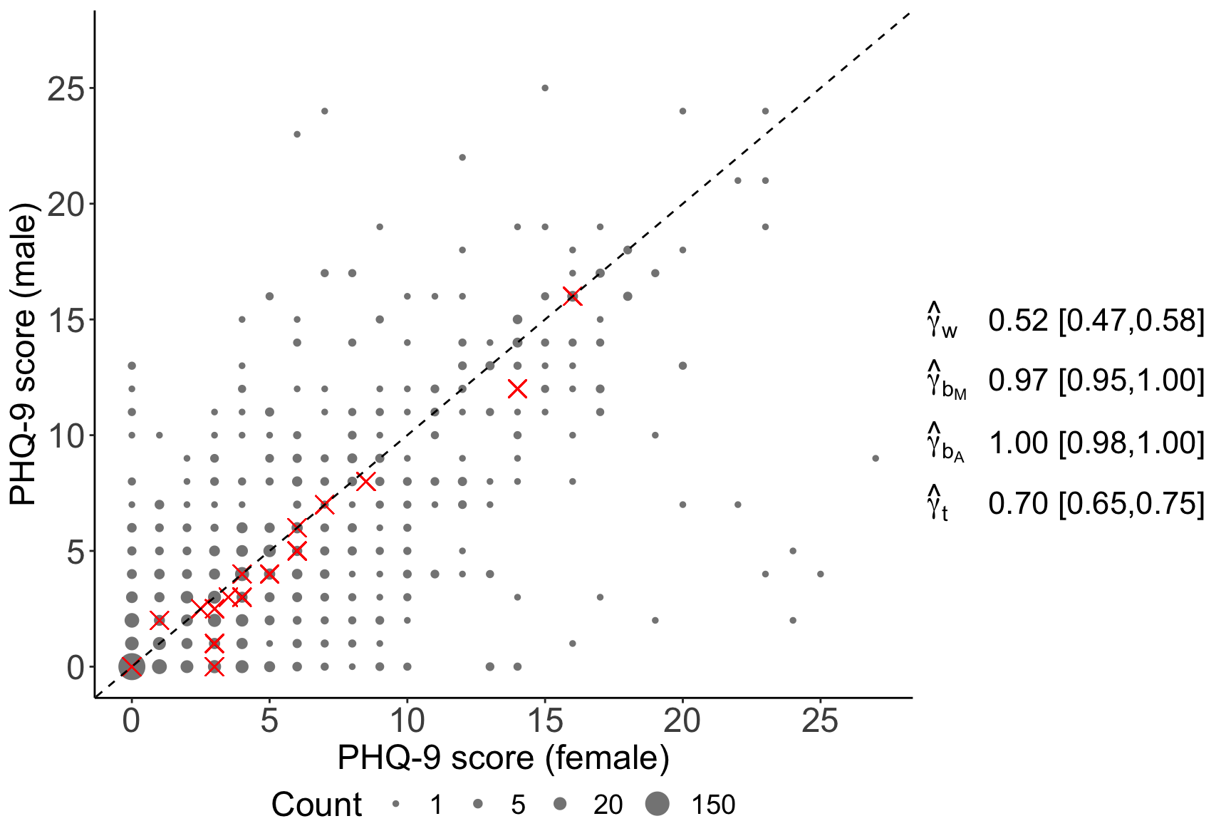
(b) PHQ-9 scores

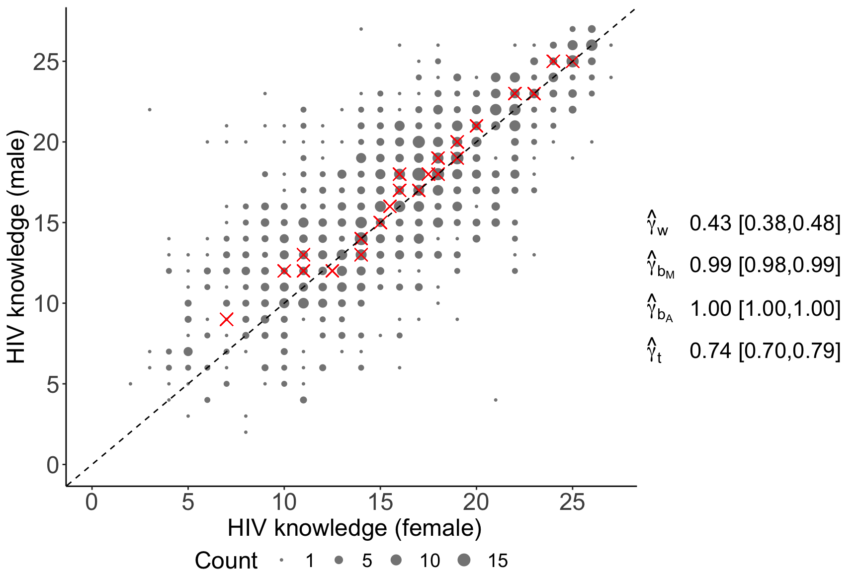
(c) HIV knowledge

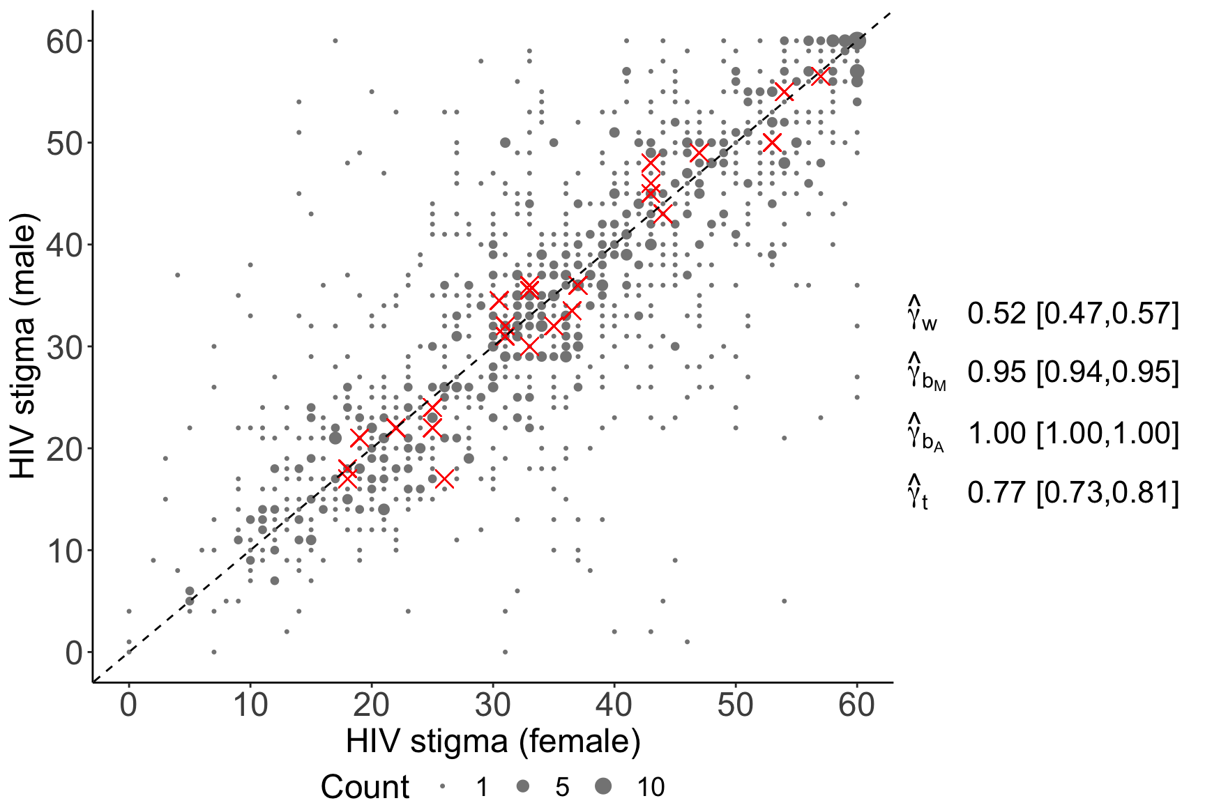
(d) HIV stigma

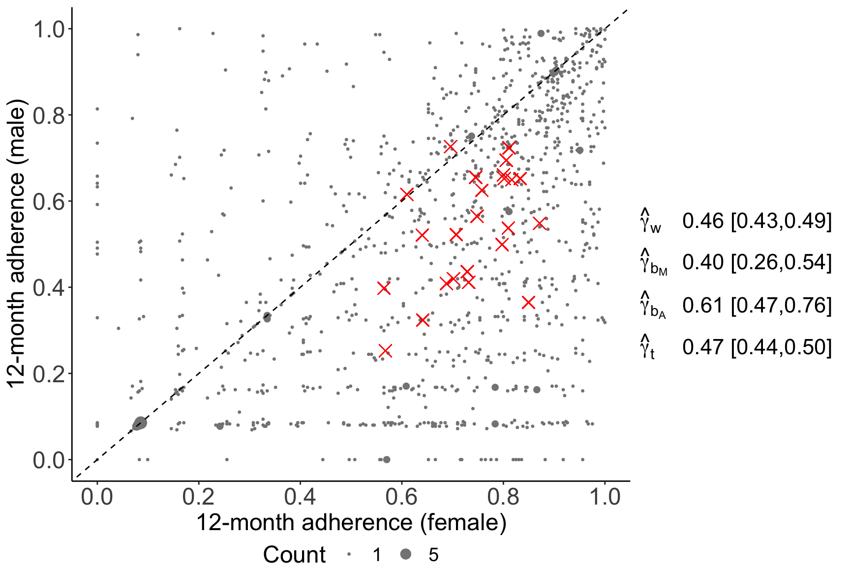
(e) 12-month adherence

Figure 4: Scatter plots of PHQ-9 scores, age at enrollment (years), HIV knowledge, HIV stigma, and 12-month adherence (%) of female and male partners enrolled in the clustered randomized clinical trial. The red cross sign represents the sample cluster median and the dot sign represents the observation. The right side of each subfigure shows the estimates of total, between-, and within-cluster Spearman rank correlations ($\gamma_{t}$, $\gamma_{b}$, $\gamma_{w}$, [$95\%$ CIs]). $\hat{\gamma}_{b_{M}}$ is the estimator of $\gamma_{b}$ based on cluster medians obtained from CPM and $\hat{\gamma}_{b_{A}}$ is the estimator of $\gamma_{b}$ based on the linear approximation.

The Homens para $\text{Sa}\acute{\text{u}}\text{de}$ Mais (HoPS+) study is a cluster randomized controlled trial in $\text{Zamb}\acute{\text{e}}\text{zia}$ Province, Mozambique (Audet et al., 2018). The trial was designed to measure the impact of incorporating male partners with HIV into prenatal care for pregnant women living with HIV on adherence to treatment. The trial enrolled 1073 participating couples living with HIV at 24 clinical sites. The number of couples at clinical sites ranged from 15 to 71. At the time of randomization (baseline), age, depressive symptoms measured by Patient Health Questionnaire-9 (PHQ-9) score, HIV knowledge, and HIV stigma were captured. We are interested in the correlation of these baseline measures within couples. We are also interested in the correlation of 12-month adherence to ART within couples. Figure 4 shows scatter plots of these measures.

In this example, the cluster is the clinical site and the observations are made on couples (e.g., $X$ = age of female partners, $Y$ = age of male partners). Hence, it is reasonable to assign equal weights to couples. The estimates of the total, between-cluster, and within-cluster Spearman rank correlations are shown in Figure 4. The total Spearman rank correlation for age, 0.59, was moderate to strong. The between-cluster Spearman rank correlation for age was $\hat{\gamma}_{b_{M}}=0.38$, suggesting weak to moderate correlation between median male and female ages within clinical sites. The within-cluster Spearman rank correlation was 0.61, implying that after controlling for clinical site, the correlation of age between couples remained high. For PHQ-9 scores, HIV knowledge, and HIV stigma, the total Spearman rank correlation between couples was strong, ranging from 0.70 to 0.77. The correlation became moderate after controlling for clinical sites, with $\hat{\gamma}_{w}$ varying from 0.43 to 0.52. The between-cluster Spearman rank correlations of the three measures were extremely strong, which can be seen in Figure 4. The approximation-based estimates ($\hat{\gamma}_{b_{A}}$) of the between-cluster correlation hit the boundary and were thus set to be 1, and the cluster-median-based estimates ($\hat{\gamma}_{b_{M}}$) were close to 1. Taken as a whole, these estimates suggest that the scores between male and female partners for these measures are highly correlated but that some of the correlation is due to similarities within sites. This may reflect differences between participants across sites or perhaps differences in the ways the questionnaires were administrated across study sites. Finally, the total correlation for 12-month adherence was moderate, 0.47. After controlling for clinical sites, the correlation remained moderate, $\hat{\gamma}_{w}=0.46$. The between-cluster correlation was moderate to high, $\hat{\gamma}_{b_{M}}=0.40$ and $\hat{\gamma}_{b_{A}}=0.61$; this difference might be due to the small intraclass correlations for this variable (the rank ICC of 12-month adherence for males was 0.06 and for females was 0.07).

9 Discussion

In this paper, we defined the population parameters of the between- and within-cluster Spearman rank correlations for clustered data, which are natural extensions of the between- and within-cluster Pearson correlations to the rank scale. We also approximated their relationship with the total Spearman rank correlation and the rank intraclass correlation coefficient. Compared with the traditional Pearson correlation, our method is insensitive to extreme values and skewed distributions, and does not depend on the scale of the data. Our framework is general, and is applicable to any orderable variables. Our estimators are asymptotically normal, with generally low bias and good coverage in our simulations. Our method requires fitting models for the conditional distributions of $X$ and $Y$ given cluster index, which need to be approximately correct to get unbiased estimates. We here suggest using semiparametric cumulative probability models which maintain the rank-based nature of Spearman’s rank correlation. We have developed an R package, rankCorr, available on CRAN, which implements our new method.

Our method has some limitations. Our method requires fitting models for the conditional distributions of $X$ and $Y$ given cluster index, which need to be approximately correct to get unbiased estimates. We suggest using semiparametric cumulative probability models which maintain the rank-based nature of Spearman’s rank correlation. In addition, our estimator of the between-cluster Spearman rank correlation has bias when the between- and within-cluster Spearman rank correlations are in opposite directions. This problem also exists when estimating the between-cluster Pearson correlation. As the cluster size increases, the problem goes away.

In practice, one may be interested in estimating covariate-adjusted rank correlations. For example, in the application of CD4 and CD8 data, there may be interest in measuring the rank correlations after adjusting for age. The methods in this manuscript could be extended to allow for covariate adjustment by fitting CPMs that include the covariate, in addition to the cluster indicators. We suspect that the correlation between probability-scale residuals from these fitted models could be used to estimate covariate-adjusted within-cluster rank correlations and that the correlation between cluster indicator coefficients from these fitted models could be used to estimate covariate-adjusted between-cluster rank correlations. This approach is somewhat similar to random effects approaches used for estimating covariate-adjusted within- and between-cluster Pearson correlations (Ferrari et al., 2005). Such an approach, as well as Spearman rank correlation as a function of time with longitudinal data, warrants further investigation.

Supplementary Materials

Web Appendices, Tables, and Figures referenced in Sections 6 and 7 are available with this paper at the Biometrics website on Wiley Online Library. We have developed an R package, rankCorr, available on CRAN, which implements our new method. The codes for simulations and applications are available on GitHub (https://github.com/shengxintu/rankCorr).

Table 1: The total, between-cluster, and within-cluster Spearman rank correlations ($\gamma_{t},\gamma_{b},\gamma_{w}$) and Pearson correlations ($\rho_{t},\rho_{b},\rho_{w}$) under Scenarios I, II, and III with 5 simulation settings

($\rho_{0t},\rho_{0b},\rho_{0w}$)	($\gamma_{t},\gamma_{b},\gamma_{w}$)		($\rho_{t},\rho_{b},\rho_{w}$)
I, II, III	I, II	III	I	II	III
(0.75, 0.80, 0.70)	(0.73, 0.79, 0.68)	(0.53, 0.79, 0.68)	(0.75, 0.80, 0.70)	(0.42, 0.61, 0.33)	(0.02, 0.03, 0)
(0.40, 0.80, 0)	(0.38, 0.79, 0)	(0.31, 0.79, 0)	(0.40, 0.80, 0)	(0.22, 0.06, 0)	(0.01, 0.02, 0)
(0.40, 0, 0.80)	(0.38, 0, 0.79)	(0.25, 0, 0.79)	(0.40, 0, 0.80)	(0.22, 0.01, 0.37)	(0, 0, 0)
(0, 0, 0)	(0, 0, 0)	(0, 0, 0)	(0, 0, 0)	(0, 0, 0)	(0, 0, 0)
(0.05, 0.80, -0.7)	(0.05, 0.79, -0.68)	(0.09, 0.79, -0.68)	(0.05, 0.80, -0.70)	(0.03, 0.59, -0.32)	(0.01, 0.01, 0)

References

- Audet et al. (2018) Audet, C. M., Graves, E., Barreto, E., De Schacht, C., Gong, W., Shepherd, B. E., et al. (2018). Partners-based HIV treatment for seroconcordant couples attending antenatal and postnatal care in rural mozambique: A cluster randomized trial protocol. Contemp Clin Trials Commun 71, 63–69.
- Bross (1958) Bross, I. D. J. (1958). How to use ridit analysis. Biometrics 14, 18–38.
- Castilho et al. (2016) Castilho, J., Shepherd, B., Koethe, J., Turner, M., Bebawy, S., Logan, J., Rogers, W., Raffanti, S., and Sterling, T. (2016). Cd4+/cd8+ ratio, age, and risk of serious noncommunicable diseases in hiv-infected adults on antiretroviral therapy. AIDS 30(6), 899–908.
- Ferrari et al. (2005) Ferrari, P., Al-Delaimy, W. K., Slimani, N., Boshuizen, H. C., Roddam, A., Orfanos, P., Skeie, G., Rodríguez-Barranco, M., Thiebaut, A., Johansson, G., Palli, D., Boeing, H., Overvad, K., and Riboli, E. (2005). An Approach to Estimate Between- and Within-Group Correlation Coefficients in Multicenter Studies: Plasma Carotenoids as Biomarkers of Intake of Fruits and Vegetables. American Journal of Epidemiology 162, 591–598.
- Fisher (1925) Fisher, R. (1925). Statistical methods for research workers. Edinburgh Oliver & Boyd.
- Harrell (2015) Harrell, F. E. (2015). rms: Regression Modeling Strategies. R package version 4.2–1.
- Hunsberger et al. (2022) Hunsberger, S., Long, L., Reese, S. E., Hong, G. H., Myles, I. A., Zerbe, C. S., Chetchotisakd, P., and Shih, J. H. (2022). Rank correlation inferences for clustered data with small sample size. Statistica Neerlandica 76, 309–330.
- Kendall (1970) Kendall, M. (1970). Rank Correlation Methods. Theory and applications of rank order-statistics. Charles Griffin.
- Kruskal (1958) Kruskal, W. H. (1958). Ordinal measures of association. Journal of the American Statistical Association 53, 814–861.
- Li and Shepherd (2012) Li, C. and Shepherd, B. E. (2012). A new residual for ordinal outcomes. Biometrika 99, 473–480.
- Liu et al. (2018) Liu, Q., Li, C., Wanga, V., and Shepherd, B. E. (2018). Covariate-adjusted spearman’s rank correlation with probability-scale residuals. Biometrics 74, 595–605.
- Liu et al. (2017) Liu, Q., Shepherd, B. E., Li, C., and Harrell Jr., F. E. (2017). Modeling continuous response variables using ordinal regression. Statistics in Medicine 36, 4316–4335.
- Pearson (1907) Pearson, K. G. (1907). On further methods of determining correlation. Cambridge University Press.
- Rosner and Glynn (2017) Rosner, B. and Glynn, R. J. (2017). Estimation of rank correlation for clustered data. Statistics in Medicine 36, 2163–2186.
- Shepherd et al. (2016) Shepherd, B., Li, C., and Liu, Q. (2016). Probability-scale residuals for continuous, discrete, and censored data. The Canadian Journal of Statistics / La Revue Canadienne de Statistique 44, 463–479.
- Shih and Fay (2017) Shih, J. H. and Fay, M. P. (2017). Pearson’s chi-square test and rank correlation inferences for clustered data. Biometrics 73, 822–834.
- Snijders and Bosker (1999) Snijders, T. and Bosker, R. (1999). Multilevel Analysis: An Introduction to Basic and Advanced Multilevel Modeling. London: Sage Publishers.
- Stefanski and Boos (2002) Stefanski, L. A. and Boos, D. D. (2002). The calculus of m-estimation. The American Statistician 56, 29–38.
- Tian et al. (2023) Tian, Y., Shepherd, B. E., Li, C., Zeng, D., and Schildcrout, J. S. (2023). Analyzing clustered continuous response variables with ordinal regression models. Biometrics 79, 3764–3777.
- Tu et al. (2023) Tu, S., Li, C., Zeng, D., and Shepherd, B. E. (2023). Rank intraclass correlation for clustered data. Statistics in Medicine 42, 4333–4348.