Graph Neural Networks for Predicting Solubility in Diverse Solvents using MolMerger incorporating Solute-solvent Interactions

Abstract

Prediction of solubility has been a complex and challenging physiochemical problem that has tremendous implications in the chemical and pharmaceutical industry. Recent advancements in machine learning methods have provided great scope for predicting the reliable solubility of a large number of molecular systems. However, most of these methods rely on using physical properties obtained from experiments and or expensive quantum chemical calculations. Here, we developed a method that utilizes a graphical representation of solute-solvent interactions using ‘MolMerger’, which captures the strongest polar interactions between molecules using Gasteiger charges and creates a graph incorporating the true nature of the system. Using these graphs as input, a neural network learns the correlation between the structural properties of a molecule in the form of node embedding and its physiochemical properties as output. This approach has been used to calculate molecular solubility by predicting the Log solubility values of various organic molecules and pharmaceuticals in diverse sets of solvents.

1 INTRODUCTION

The molecular solubility of a solute is an important property that plays a crucial role in material science, environmental chemistry, food and beverage industry, chemical process optimization, biotechnology, cosmetic formulation, agrochemicals, oil and gas Industry, and drug development. The prediction of molecular solubility of a solute in various solvents is one of the crucial challenges that attracted a lot of attention from the research community. A robust solubility model precisely forecasting solubility issues during the early stage of drug development process significantly reduces time and monetary resources. A trustworthy solubility model aids in the selection of promising drug candidates during the drug discovery process, halting the advancement of compounds with low solubility that could cause problems with formulation and or lower bio-availability. Understanding solubility patterns helps chemists create formulations with the best possible drug dissolution rates, which is essential for both drug efficacy and patient outcomes.

Solubility prediction has been a long-standing problem^{1, 2, 3}, and over the years a plethora of methods have been developed to predict solubility of molecular systems.^{4, 5, 6, 7, 8, 9, 10, 11, 12, 13, 14, francoeu2021soltrannet, 15, 16, 17} Among the recent ML-based methods, Graph Neural Networks (GNNs), including Graph Convolution Networks (GCN), Message Passing Neural Networks (MPNN), Graph Attention Networks (GATs), and Attentive Finger Printing (AFP) have gained enormous popularity due to their inherent capability of embedding structural properties of molecules as graphs.^{18, 19, 20, 21, 22, 23, boobie2020machine, 24, 25, 26, 27} These methods mostly utilize structural as well as experimentally obtained physicochemical properties to predict the solubility of molecular systems. Additionally, they are limited to predicting aqueous solubility except in a handful of cases where non-aqueous solvents have been considered. In a recently proposed method, Lee et al. incorporated solute-solvent pairs in a GCN, which passes both the solute and solvent information through convolution layers and passes them through a Multi-Layer Perceptron (MLP) by concatenating them into a single one-dimensional embedding, as input neurons.²⁴ The problem with this approach is that, with a complex neural network, the model categorizes solubilities by solvent and recognizes patterns using the solvents in the training set. When a new solvent is introduced, the model fails, due to its over-fitting to known solvents. Thus there has been a need for developing a new method that can incorporate physical interactions between solute and solvent without overfitting or categorizing solubility to specific solvents, and while message passing, the interactions between the solute and solvent, such as polar, hydrogen, or ionic interactions can be included in the input graph.

In this work, we have developed a GNN-based model that takes into account explicitly the solute-solvent interactions and provides reliable solubility of a large number of organic molecules including active pharmaceuticals in both aqueous and organic solvents. The solute-solvent interactions have been incorporated by a graph ‘MolMerger’, which by using Gastieger charges²⁸ incorporates interactions between two polar, partially charged atomic centers in the solute and solvent molecules. This way the GNN learns the correlation between the structures of solute and solvent molecules as well as their physical interactions, thereby providing accurate solubility values for a solute in several solvents.

2 METHODS

2.1 Training Data

We have collated the dataset (total size of 5198) from three different sources - BigSolDB²⁹, BNNLabs Solubility, and ESOL³⁰. Our aim here is to keep a limited set of solvents while training and evaluate a larger set of solvents to see the efficiency of the model, and if the model can predict never-seen-before solvents. The most number of data entries in Table 1 are from BigSolDB. The 13 solvents each having solutes ranging from 127 to 1212. The descriptor used is the canonical SMILES representation. Each solute-solvent pair was converted to a Molecular Fingerprint using RDKit Library in Python.

The data collected from BigSolDB needed to be cleaned to avoid false and bad data from the database. The BigSolDB dataset has solubilities for a solute-solvent pair at 1 to 15 different temperatures. The solute-solvent pairs were grouped. For each pair, solubilities were plotted against temperature. On inspection, it was observed that a large set of solute-solvent pairs had random data points with redundant values as shown in Figure 1. Some solvents had more than one LogS value for each solute at different temperatures. Since a manual inspection is not possible for a dataset of 50000 data points, a robust non-biased algorithm was applied. A regression was fit to each solute-solvent pair, with a general formula:

$$S=ae^{bT}$$ (1)

where $S$ is solubility, and $a$ and $b$ are parameters discussed in article³¹.

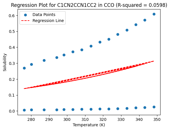
Figure 1: Examples of erroneous data points in the dataset.

Solute-solvent pairs with $R^{2}$ accuracy of less than 0.925 were removed, constituting less than 2% of the data. These 2% plots were manually inspected to ensure no loss of valuable data takes place. Further, both solute and solvent were converted to an RDKit molecule using the ‘MolFromSmiles’ method, and SMILES with errors were removed. SMILES with more than one molecule represented by a ”.” were also discarded. Solvents with a solute frequency greater than 120 were used for training (split into the train and test sets), and less than 120 and greater than 2 were kept for a robust evaluation on a broader set. Finally, the LogS value of a solute-solvent pair, at a temperature closest to 273K was used. It is important to note that, even optimization was done using metrics on the test set isolated from the training set, which ensures the evaluation data is untouched.

The distributions of the LogS values in the training and the evaluation datasets are shown in Figure 2. The most probable values of LogS range from -4.5 to 0 in both the training and evaluation datasets.

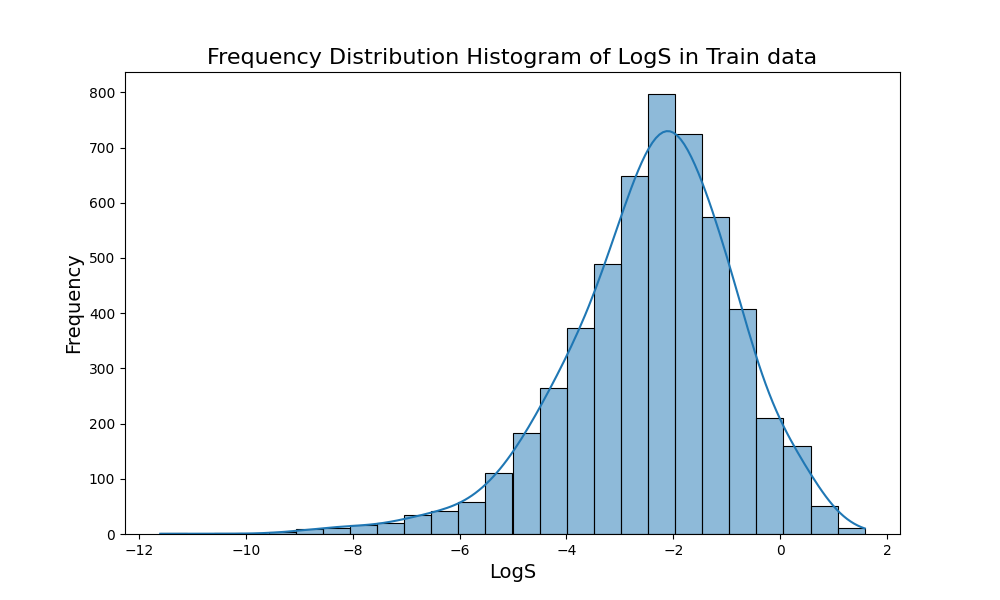
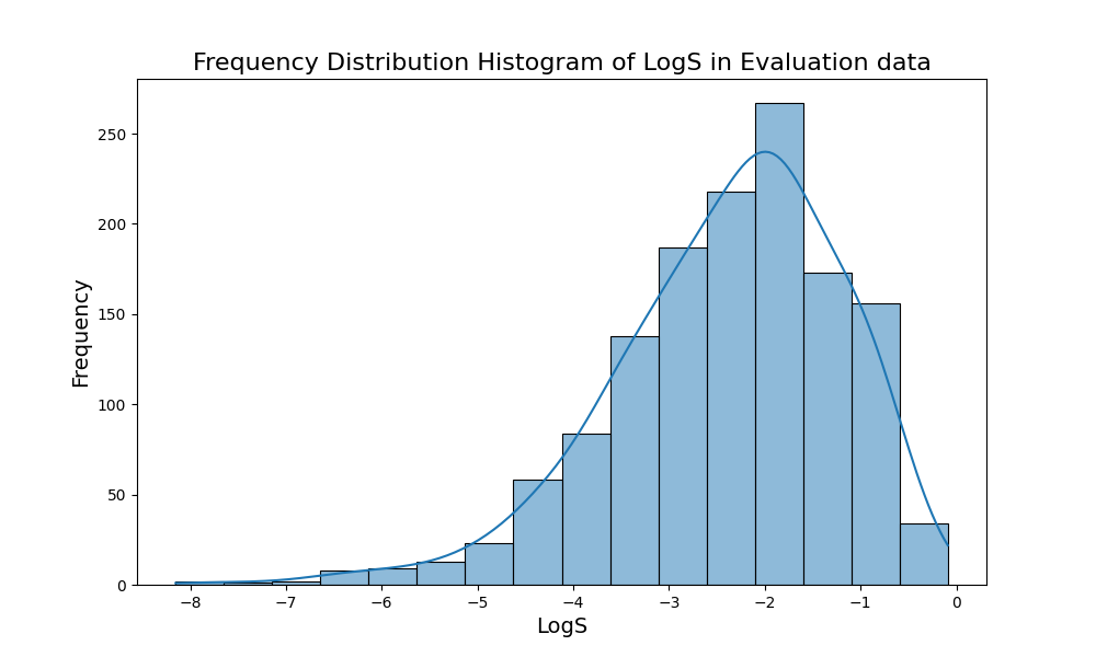
Figure 2: The distributions of the LogS values in the (a) training and (b) evaluation datasets.

Serial No.	Source	No. of Solvents	No. of Data Entries	% of total data
1	BigSolDB	10	3126	60.1%
2	BNNLabs Solubility	2	1093	21.0%
3	ESOL	1	979	18.9%

Table 1: Sources for Data

Serial No.	Solvent SMILES	Solvent Name	Solute Frequency
1	C1COCCO1	Tetrahydrofuran	127
2	CC#N	Acetonitrile	237
3	CC(=O)C	Acetone	427
4	CC(C)=O	Acetaldehyde	299
5	CC(C)O	Ethanol	329
6	CCCCCO	Hexane	255
7	CCCO	Propanone	274
8	CCO	Ethylene glycol	1079
9	CCOC(C)=O	Ethyl acetate	331
10	CN(C)C=O	DMF	128
11	CO	Carbon monoxide	366
12	Cc1ccccc1	Toluene	134
13	O	Water	1212

Table 2: Solvents and Solute Frequency in Train Data

2.2 Features of Graph and Graph Representation

Graph Neural networks (GNNs) work in a way that makes it convenient to feed graph data to a neural network. A graph in Graph Neural Networks (GNNs) is represented as $G=(V,E)$, where $V$ is the set of nodes (vertices) representing entities or elements in the graph, and $E$ is the set of edges representing relationships or connections between nodes. In the case of molecular systems, the atoms are described as nodes while the bonds are represented by edges. Graph representations not only make it easier to describe molecules, but attentive weights assigned to edges after message passing, help find the important regions in the graph by assigning higher weights, whereas less important sections of the graph with lower weights. In our case, only graph-level features and no global embedding have been used, which helps in finding the correlation between just the structural properties of a molecule and its property - the solubility.

Serial No.	Feature Name	Feature Size	Feature Description
1)	Type of Atom	10	A vector of 1s and 0s for atom type. Set of Atoms = [“C”, “N”, “O”, “F”, “P”, “S”, “Cl”, “Br”, “I”, Unknown]
2)	Hybridisation	3	A vector of 1s and 0s for hydridisations. Set of Hybridisations = [”SP1”, ”SP2”. ”SP3”]
3)	Formal Charge	1	A vector of a float value of formal charge. Set of attribute = [”Formal Charge”]
4)	Acceptor/Donor	2	A vector of 1s and 0s of electronic behavior. Set of attributes = [”Acceptor”, ”Donor”]
5)	In Aromatic	1	A vector of 1s and 0s for aromaticity. Set of attribute = [”Is in Aromatic System”]
6)	Degree	7	A vector of 1s and 0s for degree of atom. Set of Degrees = [”0”, ’1”, ”2”, ”3”, ”4”, ”5”, Unknown]
7)	Chirality	2	A vector of 1s and 0s for chiral behavior. Set of Chiralities = [”R”, ”S”]
8)	No of Hydrogens	5	A vector of 1s and 0s for hydrogens on atom. Set of count = [”0”, ”1”, ”2”, ”3”, ”4”]

Table 3: Node Features of Graph- Properties of atom

Serial No.	Feature Name	Feature Size	Feature Description
1)	Type of Bond	5	A vector of 1s and 0s for bond type. Set of bonds = [“SINGLE”, “DOUBLE”, “TRIPLE”, “AROMATIC”, ”HYDROGEN” or Unknown]
2)	Is in same ring	1	A vector of 1s and 0s for is in same ring as atom. Set of attributes = [”Is in the ring”]
3)	Is in Conjugation	1	A vector of 1s and 0s for is in conjugation. Set of attribute = [”is in conjugation”]
4)	Stereo Configuration	2	A vector of 1s and 0s for stereochemistry of bond. Set of attributes = [“STEREONONE”, “STEREOANY”, “STEREOZ”, “STEREOE”, Unknown]
5)	Graph Distance	1	A vector of 1s and 0s for graph distance. Set of attribute = [“1”, ”2” … ”7”, higher]

Table 4: Edge Features of Graph- Properties of bond

A featurizer has been used to transform the 2D molecular structure into an object representation suitable as an input for the GNN. The object has three attributes - (1) node features (see Table 3), (2) edge features (Table 4), and (3) edge weights in the form of an adjacency Matrix. This adjacency matrix is used as a mask that represents connected nodes in a Graph. Most research on physiochemical properties prediction using Machine Learning and Deep Learning methods such as in Ref.32, obtained commendable results, however, they mostly rely on using experimental data such as zero-point energies, solvation energies, Gibbs free energies, dipole moments, and solvent accessible surface area as features. Though these features increase accuracy, they are obtained from expensive quantum chemical calculations or sophisticated experiments. In our approach, we rely on using only the structural information of a molecule along with a Site-Charge (SC) description (discussed in the subsequent section) with no trivial correlation to solubility that can be computed from basic chemistry, without quantum calculations, MD simulations, and or experiments.

2.3 Solute-solvent interactions: Site-Charge (SC) model

Incorporation of solvent details into the NN model is crucial, especially, when one wants to calculate the solubility of a solute in different solvents. In Ref.24, Lee et al. studied a combination of solute and solvents to predict solubility by using a multi-input network model with solute and solvent fingerprints (GCNs). They showed that in addition to using two GCNs for solute and solvent, the inclusion of physicochemical property-based features improves the solubility prediction. This model, however, relies on internally classifying the solute-solvent pairs based on solvent properties. While this provides satisfactory results in terms of predicting the solubility, the models encounter limitations when a completely new solvent is considered. One way of avoiding this issue is to have a model that can learn solute-solvent interactions and predict solubility without exclusively knowing the structure of the solvent molecule.

Here, we have introduced a new way to incorporate solute-solvent interactions and the method we named ‘MolMerger’. The MolMerger algorithm takes in the RDKit 2D molecular representation of a solute and solvent and iterates over each atom in both molecules independently. (Figure 3) During this iteration, the algorithm calculates the atomic partial charges using the Gastieger charges method as shown in Ref. 28. Table 5 shows the algorithm deployed for the calculation.

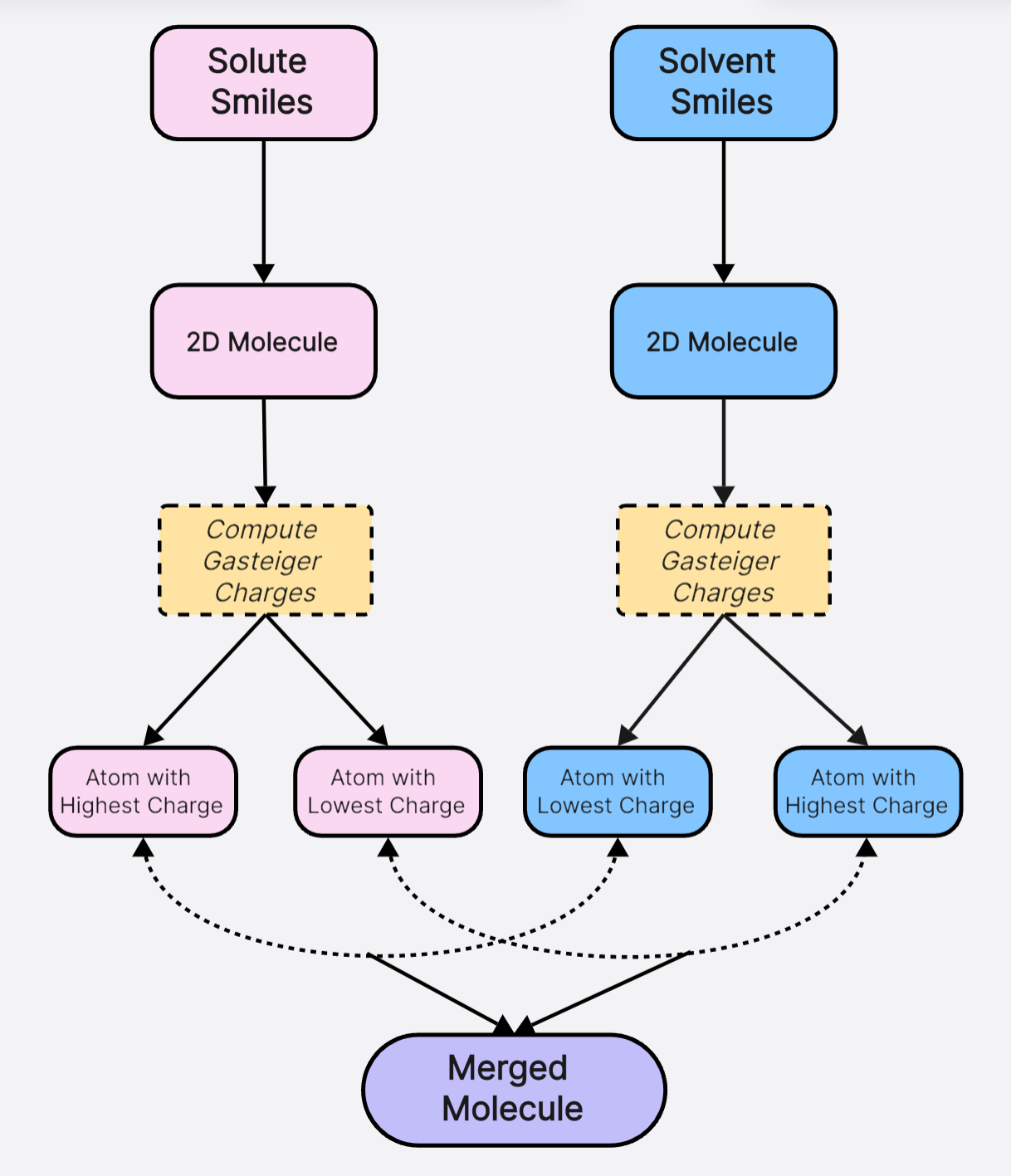
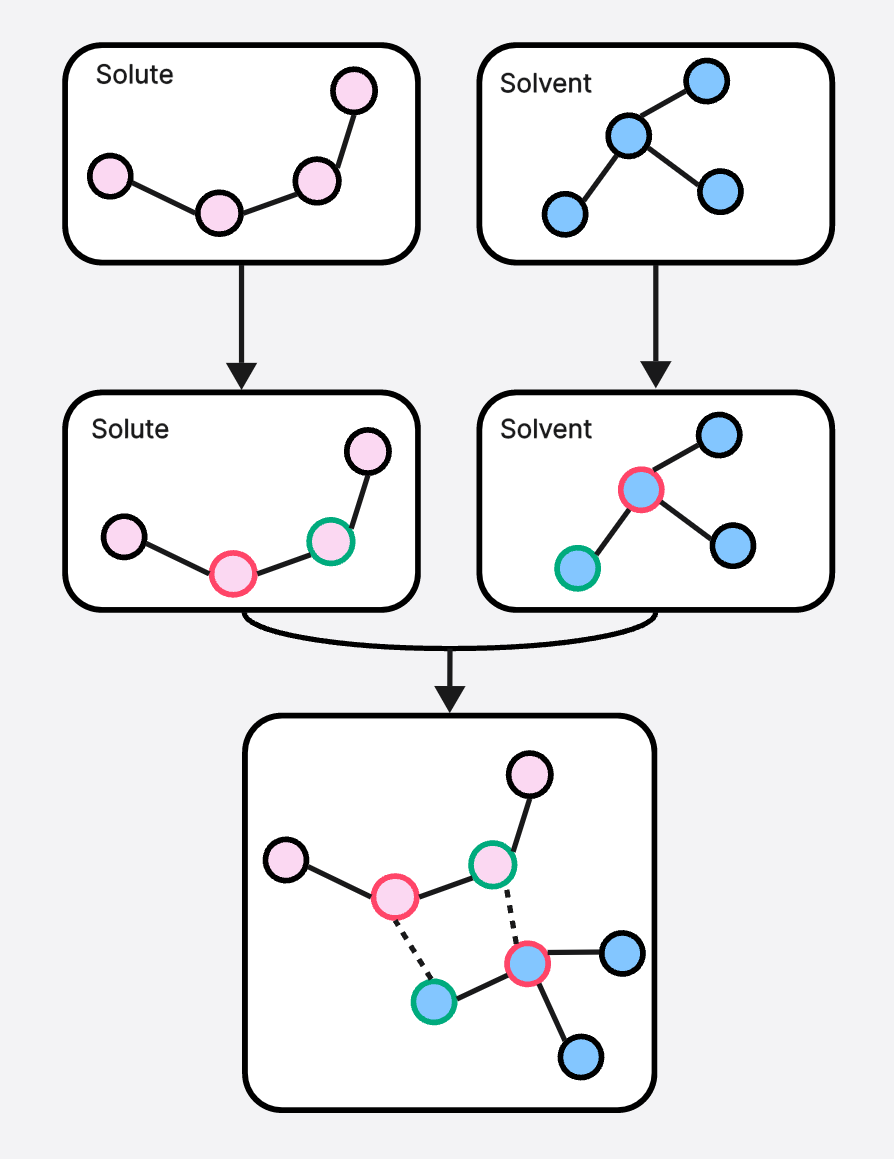
Figure 3: a) FlowChart of MolMerger Algorithm b) Depiction of working of MolMerger

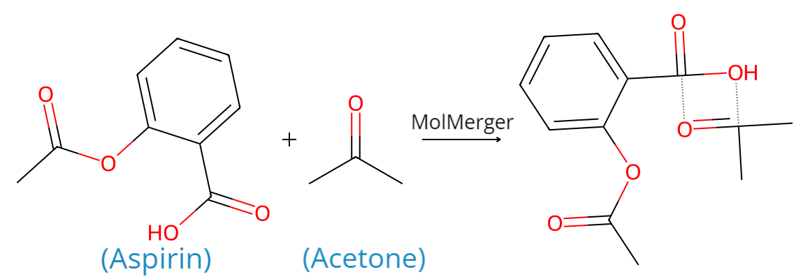
Figure 4: Example showing MolMerger working on Aspirin and Acetone.

Step	Equation	Target
Initial charges:	$q_{i}=Z_{i}+\sum_{j\neq i}\dfrac{Z_{j}}{R_{ij}}$	Assigns seed charges based on atomic number and neighboring atoms. Initial charge $q_{i}$ for atom $i$.
Charge redistribution:	$q_{i,k}=q_{i,k-1}+\alpha_{i}\left(\sum_{j\neq i}\dfrac{q_{j,k-1}}{R_{ij}^{2}}-\rho_{i}\right)$ $\alpha_{i}=\dfrac{1}{1+\gamma_{i}\left|q_{i,k-1}\right|}$	Redistributes charges based on electronegativities and orbital configurations iteratively until convergence.
Partial charges:	$q_{i}=Z_{i}+\sum_{j\neq i}q_{j}$	Final charges model electrostatic properties.

Table 5: Gasteiger Charges Method Steps

Variable	Meaning
$Z_{i}$	Atomic number of atom $i$
$R_{ij}$	Distance between atoms $i$ and $j$
$q_{i}$	Charge of atom $i$
$q_{i,k}$	Charge of atom $i$ at iteration $k$
$\alpha_{i}$	Scaling factor for charge redistribution of atom $i$
$\gamma_{i}$	Damping factor for controlling convergence rate
$\rho_{i}$	Electronegativity of atom $i$

Table 6: Variables and Meanings in Gasteiger Charge Method

The atoms in solute and solvent with the highest and lowest Gasteiger charges are tagged, and a ‘virtual’ bond is formed between the most electron-dense atom in the solute to the least electron-dense atom in the solvent, and vice versa. This approach captures and simplifies the complex polar interactions between solute-solvent molecules into two bonds in a new ‘Merged-Molecule’. The two virtual bonds thus created between the solute and solvent make the Merged-Molecule unique for a specific solute-solvent pair.

2.4 Model Description

For the prediction of LogS after featurization on the merged molecule, the graph obtained is fed to a model with architecture based on the AttentiveFP model as described in Ref.33. The AttentiveFP model is a GNN model for molecular representation learning as depicted in Figure 5. It is implemented in PyTorch Geometric and consists of the following components:

• A linear layer that maps the input feature dimensionality to the hidden feature dimensionality.

• A GATEConv layer (gate-conv) that updates the node features based on the edge features and the previous node features.

• A GRU cell (gru) that updates the node features based on the output of the GATEConv layer.

• A list of GATConv layers (atom-convs) and GRU cells (atom-grus) that further update the node features.

• A GATConv layer (mol-conv) that generates a molecular embedding by pooling the updated node features.

• A GRU cell (mol-gru) that further updates the molecular embedding.

• A linear layer that maps the molecular embedding to the output feature dimensionality.

The model takes as input the node features (x), edge indices (edge-index), and edge features (edge-attr), as well as a batch vector (batch) that defines the molecular structure of the input data. It outputs a vector representation of each molecule. The forward method applies a series of graph convolution and GRU operations to the node and molecular features and uses dropout for regularization. The reset-parameters method resets the learnable parameters of the model to their initial values.

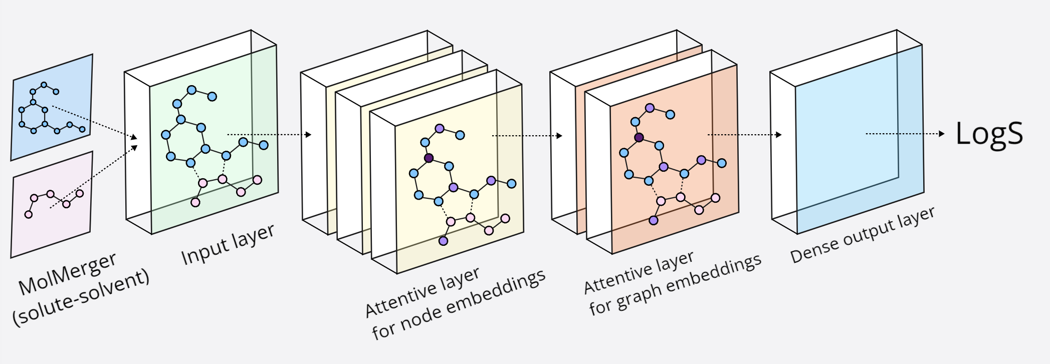
Figure 5: AttentiveFP model architecture

2.5 Attentive Fingerprinting

The AttentiveFP model³³ is built on the Graph Attention Mechanism, which allows it to focus on the most relevant parts of the molecular graph when generating a molecular representation. By weighing the importance of different parts of the graph, the model can better capture the complex relationships between atoms and bonds in a molecule. (Figure 6) This is in contrast to traditional GNNs, which treat all parts of the graph equally and may not be as effective at capturing the nuanced relationships in molecular graphs. The AttentiveFP uses gated recurrent units (GRUs) as it allows for the modeling of temporal dependencies in the graph-level molecular embedding. The GRU cell updates the molecular embedding based on the output of the GATConv layer, which captures the structural and chemical properties of the molecule at the atom level. By incorporating a GRU cell, AttentiveFP can capture how these atom-level properties evolve, which can be important for modeling certain molecular properties. In comparison to GAT, AttentiveFP may be better at capturing temporal dependencies in the data.

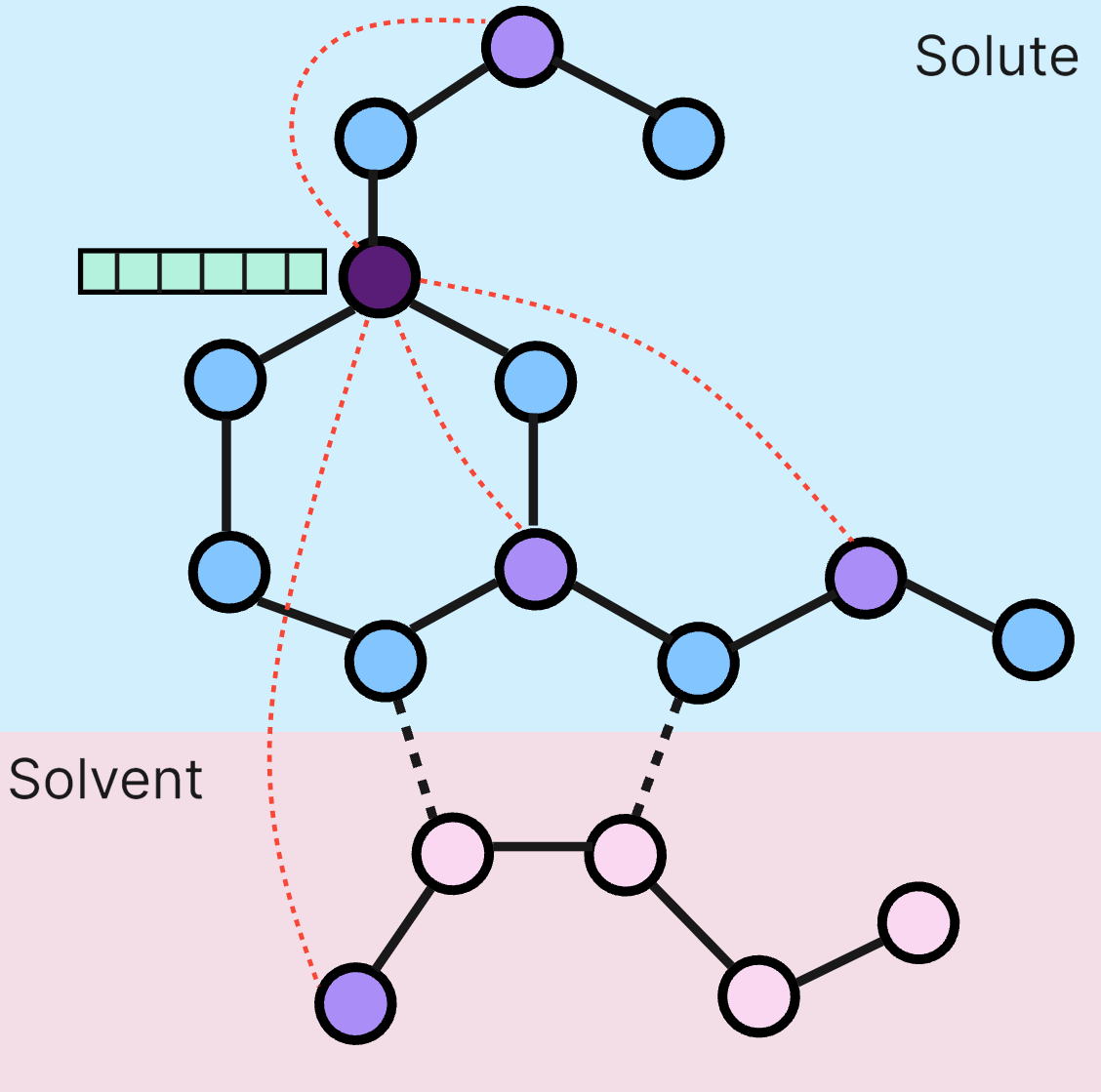
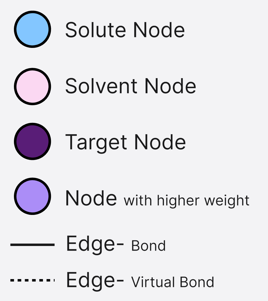
Figure 6: Depiction of attention context passing from nodes in solvent to target node in solute incorporating solute-solvent interactions

2.6 Loss Function and Hyperparameters

For the regression task of LogS prediction, L2Loss was used. Whereas for the Classification task, Sparse Softmax CrossEntropy with Logits (SSCE) was used as described in equations 2 and 3:

L2 Loss: $$\quad L(\hat{y},y)=\sum_{i=1}^{n}\frac{1}{2}\lVert\hat{y}-y\rVert^{2}$$ (2)

SSCE Loss: $$\quad L_{\text{SSCE}}(\mathbf{z},\mathbf{y})=-\sum_{i}y_{i}\log\left(\frac{e^{z_{i}}}{\sum_{j}e^{z_{j}}}\right)$$ (3)

$$\mathbf{z}$$ : input logits

$$\mathbf{y}$$ : sparse ground truth label vector.

The number of layers for Graph Attention, the number of time steps, and the number of epochs are the model’s hyperparameters. The number of layers and time steps are important for the internal architecture of the model, which determines the complexity of the model. It is worth noting that a more complex model is not necessarily better, as a huge amount of data is required to fit the parameters. The number of epochs must be optimized based on the loss in the test data, to avoid over-fitting to the train data.

3 RESULTS AND DISCUSSION

The GNN-based solubility prediction model demonstrated robust performance in the prediction of molecular solubility. (Figure 7) The key performance metrics, including mean absolute error (MAE), $R^{2}$ Score, and other relevant evaluation metrics are provided in Figures 7, 8 and 9, respectively. The model’s accuracy is evident from its ability to closely match experimental solubility values across a diverse set of solute-solvent pairs. (Table X) Evaluation of 55 solvents showed an average loss (MAE of each solvent) of 0.7501. 80% solvents (44 solvents) having MAE less than 1 and 58% solvents with MAE less than 0.75. The average $R^{2}$ score is 0.59, but we notice the $R^{2}$ value is not the best indicator of the model’s performance, for fewer data points in each solvent as it is highly sensitive to outliers and can be significantly affected by a few data points with extreme values, leading to an inaccurate assessment of the model’s performance.

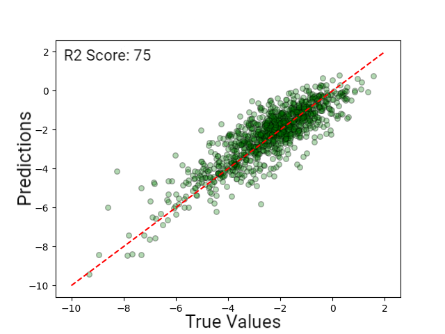
Figure 7: Predicted vs experimental LogS values on test set

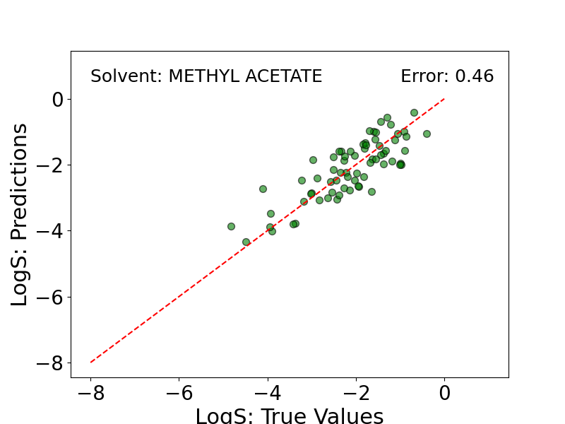
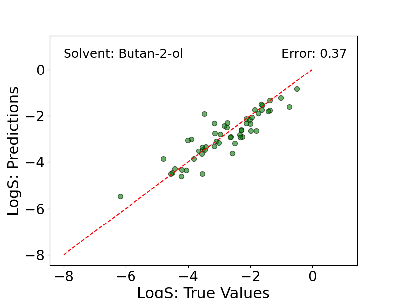
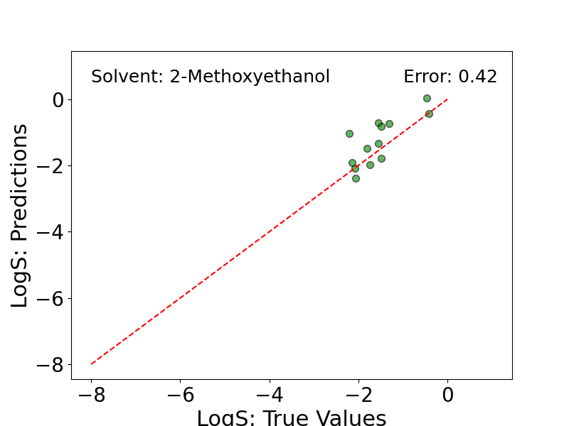
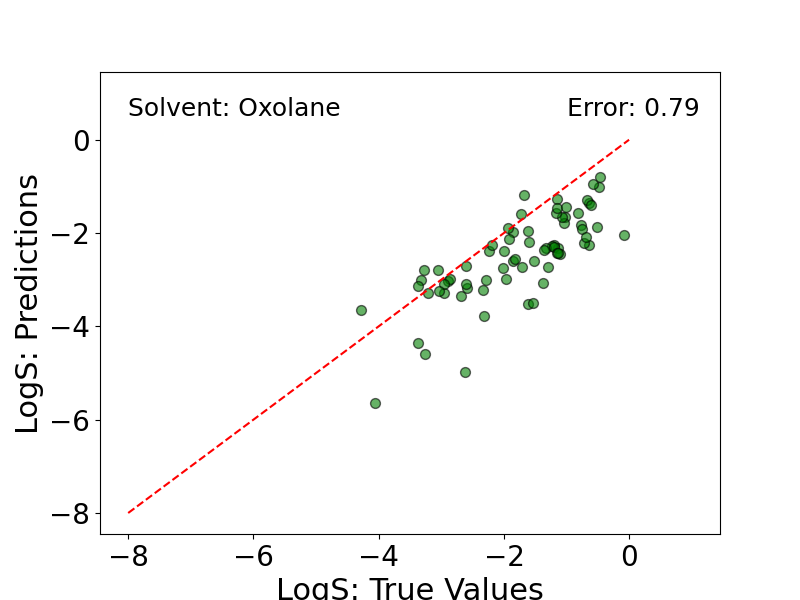
Figure 8: Predicted vs. experimental LogS values of a few pharmaceutically important solvents

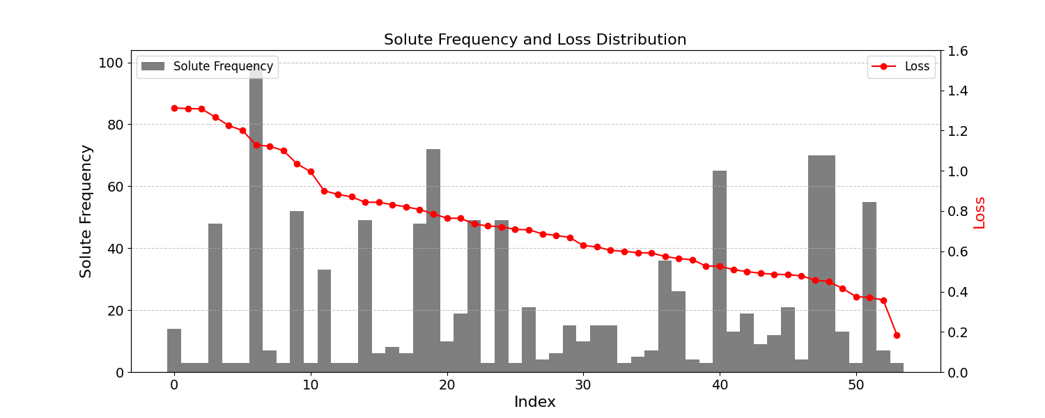
Figure 9: Solute Frequency and Loss (MAE) for each solvent by index

Finally, in Table 7, we provided the solubility of a few popular drug molecules predicted using our model and compared them with the experimental values. The predicted solubility values are close to the experimental values manifesting the effectiveness of our model.

Index	Molecule Name	Solvent	Predicted LogS	Expt. LogS
1)	Aspirin	Water	-2.806	-2.699
6)	Aspirin	Acetone	-0.101	0.025
2)	Paracetamol	Water	-2.052	-2.179
8)	Paracetamol	Methanol	-1.392	-1.387
3)	Amlodipine	Water	-5.486	-5.611
4)	Alprazolam	Water	-5.958	-5.489
5)	Metoprolol	Water	-4.981	-4.535
7)	Metformin	Water	-1.503	-1.744
9)	Diazepam	Methanol	-2.406	-2.699

Table 7: Solubility values - predicted and experimental for some common drugs

4 CONCLUSIONS

We proposed a new method of predicting solubility that explicitly utilizes structural information of solutes and solvents and their interactions. The MolMerger algorithm provides a unique way of incorporating solute-solvent intermolecular interactions by calculating the Gasteiger charges and finding the most polar sites in the solute and solvent molecules. This method does neither need any input data from expensive quantum chemical calculations nor data from experiments. The presented method is not limited to predicting the solubility of a solute in a specific or a small set of solvents, rather it covers a large range of solute-solvent combinations predicting their solubility with an accuracy range $\sim$50-80 %. The presented method can be improved further by incorporating more meaningful solvent interactions and temperature. Furthermore, molecular dynamics simulations-based methods^{12, 13, 15, 16, 17} can also be augmented with the proposed prediction model to calculate realistic solubility of ionic and molecular crystals.

5 ASSOCIATED CONTENT

Data Availability Statement
The codes and datasets can be found in a public GitHub repository (https://github.com/).

6 AUTHOR INFORMATION

Corresponding Author:
Tarak Karmakar
Department of Chemistry, Indian Institute of Technology,
Delhi 110016, New Delhi, India;
orcid.org/0000-0002-8721-6247;
Phone:+91 11 26548549; Email: tkarmakar@chemistry.iitd.ac.in

Authors
Vansh Ramani
Department of Chemical Engineering, Indian Institute of Technology,
Delhi 110016, New Delhi, India;

Notes:
The authors declare no competing financial interest.

7 ACKNOWLEDGEMENTS

T.K. acknowledges the Science and Engineering Research Board (SERB), New Delhi, India for the Start-up Research Grant (File No. SRG/2022/000969). We also acknowledge IIT Delhi for the Seed Grant.

References

- Llinàs et al. 2008 Llinàs, A.; Glen, R. C.; Goodman, J. M. Solubility challenge: can you predict solubilities of 32 molecules using a database of 100 reliable measurements? Journal of chemical information and modeling 2008, 48, 1289–1303
- Hewitt et al. 2009 Hewitt, M.; Cronin, M. T.; Enoch, S. J.; Madden, J. C.; Roberts, D. W.; Dearden, J. C. In silico prediction of aqueous solubility: the solubility challenge. Journal of chemical information and modeling 2009, 49, 2572–2587
- Llinas et al. 2020 Llinas, A.; Oprisiu, I.; Avdeef, A. Findings of the second challenge to predict aqueous solubility. Journal of chemical information and modeling 2020, 60, 4791–4803
- Hildebrand and Scott 1950 Hildebrand, J. H.; Scott, R. L. The solubility of nonelectrolytes. (No Title) 1950,
- Klamt et al. 2002 Klamt, A.; Eckert, F.; Hornig, M.; Beck, M. E.; Bürger, T. Prediction of aqueous solubility of drugs and pesticides with COSMO-RS. Journal of computational chemistry 2002, 23, 275–281
- Sanghvi et al. 2003 Sanghvi, T.; Jain, N.; Yang, G.; Yalkowsky, S. H. Estimation of aqueous solubility by the general solubility equation (GSE) the easy way. QSAR & Combinatorial Science 2003, 22, 258–262
- Hansen 2007 Hansen, C. M. Hansen solubility parameters: a user’s handbook; CRC press, 2007
- Delaney 2005 Delaney, J. S. Predicting aqueous solubility from structure. Drug discovery today 2005, 10, 289–295
- Dearden 2006 Dearden, J. C. In silico prediction of aqueous solubility. Expert opinion on drug discovery 2006, 1, 31–52
- Louis et al. 2010 Louis, B.; Agrawal, V. K.; Khadikar, P. V. Prediction of intrinsic solubility of generic drugs using MLR, ANN and SVM analyses. European journal of medicinal chemistry 2010, 45, 4018–4025
- Gupta et al. 2011 Gupta, J.; Nunes, C.; Vyas, S.; Jonnalagadda, S. Prediction of solubility parameters and miscibility of pharmaceutical compounds by molecular dynamics simulations. The Journal of Physical Chemistry B 2011, 115, 2014–2023
- Liu et al. 2016 Liu, S.; Cao, S.; Hoang, K.; Young, K. L.; Paluch, A. S.; Mobley, D. L. Using MD simulations to calculate how solvents modulate solubility. Journal of chemical theory and computation 2016, 12, 1930–1941
- Li et al. 2018 Li, L.; Totton, T.; Frenkel, D. Computational methodology for solubility prediction: Application to sparingly soluble organic/inorganic materials. The Journal of chemical physics 2018, 149
- Alsenz and Kuentz 2019 Alsenz, J.; Kuentz, M. From quantum chemistry to prediction of drug solubility in glycerides. Molecular pharmaceutics 2019, 16, 4661–4669
- Bjelobrk et al. 2021 Bjelobrk, Z.; Mendels, D.; Karmakar, T.; Parrinello, M.; Mazzotti, M. Solubility prediction of organic molecules with molecular dynamics simulations. Crystal Growth & Design 2021, 21, 5198–5205
- Bjelobrk et al. 2022 Bjelobrk, Z.; Rajagopalan, A. K.; Mendels, D.; Karmakar, T.; Parrinello, M.; Mazzotti, M. Solubility of Organic Salts in Solvent–Antisolvent Mixtures: A Combined Experimental and Molecular Dynamics Simulations Approach. Journal of Chemical Theory and Computation 2022, 18, 4952–4959
- Reinhardt et al. 2023 Reinhardt, A.; Chew, P. Y.; Cheng, B. A streamlined molecular-dynamics workflow for computing solubilities of molecular and ionic crystals. The Journal of Chemical Physics 2023, 159
- Lusci et al. 2013 Lusci, A.; Pollastri, G.; Baldi, P. Deep architectures and deep learning in chemoinformatics: the prediction of aqueous solubility for drug-like molecules. Journal of chemical information and modeling 2013, 53, 1563–1575
- Coley et al. 2017 Coley, C. W.; Barzilay, R.; Green, W. H.; Jaakkola, T. S.; Jensen, K. F. Convolutional embedding of attributed molecular graphs for physical property prediction. Journal of chemical information and modeling 2017, 57, 1757–1772
- Withnall et al. 2020 Withnall, M.; Lindelöf, E.; Engkvist, O.; Chen, H. Building attention and edge message passing neural networks for bioactivity and physical–chemical property prediction. Journal of cheminformatics 2020, 12, 1–18
- Cui et al. 2020 Cui, Q.; Lu, S.; Ni, B.; Zeng, X.; Tan, Y.; Chen, Y. D.; Zhao, H. Improved prediction of aqueous solubility of novel compounds by going deeper with deep learning. Frontiers in oncology 2020, 10, 121
- Tang et al. 2020 Tang, B.; Kramer, S. T.; Fang, M.; Qiu, Y.; Wu, Z.; Xu, D. A self-attention based message passing neural network for predicting molecular lipophilicity and aqueous solubility. Journal of cheminformatics 2020, 12, 1–9
- Gao et al. 2020 Gao, P.; Zhang, J.; Sun, Y.; Yu, J. Accurate predictions of aqueous solubility of drug molecules via the multilevel graph convolutional network (MGCN) and SchNet architectures. Physical Chemistry Chemical Physics 2020, 22, 23766–23772
- Lee et al. 2022 Lee, S.; Lee, M.; Gyak, K.-W.; Kim, S. D.; Kim, M.-J.; Min, K. Novel Solubility Prediction Models: Molecular Fingerprints and Physicochemical Features vs Graph Convolutional Neural Networks. ACS omega 2022, 7, 12268–12277
- Lee et al. 2023 Lee, S.; Park, H.; Choi, C.; Kim, W.; Kim, K. K.; Han, Y.-K.; Kang, J.; Kang, C.-J.; Son, Y. Multi-order graph attention network for water solubility prediction and interpretation. Scientific Reports 2023, 13, 957
- Panapitiya et al. 2022 Panapitiya, G.; Girard, M.; Hollas, A.; Sepulveda, J.; Murugesan, V.; Wang, W.; Saldanha, E. Evaluation of deep learning architectures for aqueous solubility prediction. ACS omega 2022, 7, 15695–15710
- Ahmad et al. 2023 Ahmad, W.; Tayara, H.; Chong, K. T. Attention-Based Graph Neural Network for Molecular Solubility Prediction. ACS omega 2023, 8, 3236–3244
- Gasteiger and Marsili 1980 Gasteiger, J.; Marsili, M. Iterative partial equalization of orbital electronegativity—a rapid access to atomic charges. Tetrahedron 1980, 36, 3219–3228
- Krasnov et al. 2023 Krasnov, L.; Mikhaylov, S.; Fedorov, M. V.; Sosnin, S. BigSolDB: Solubility Dataset of Compounds in Organic Solvents and Water in a Wide Range of Temperatures. ChemRxiv 2023,
- Delaney 2004 Delaney, J. S. ESOL: Estimating Aqueous Solubility Directly from Molecular Structure. Journal of Chemical Information and Computer Sciences 2004, 44, 1000–1005, PMID: 15154768
- Black and Muller 2010 Black, S.; Muller, F. On the Effect of Temperature on Aqueous Solubility of Organic Solids. Organic Process Research & Development 2010, 14, 661–665
- Boobier et al. 2020 Boobier, S.; Hose, D. R. J.; Blacker, A. J.; Nguyen, B. Machine learning with physicochemical relationships: solubility prediction in organic solvents and water. Nature Communications 2020, 11
- Xiong et al. 2019 Xiong, Z.; Wang, D.; Liu, X.; Zhong, F.; Wan, X.; Li, X.; Li, Z.; Luo, X.; Chen, K.; Jiang, H.; Zheng, M. Pushing the Boundaries of Molecular Representation for Drug Discovery with the Graph Attention Mechanism. Journal of Medicinal Chemistry 2019, 63, 8749–8760