Energy-saving fast-forward scaling

Abstract

We propose energy-saving fast-forward scaling. Fast-forward scaling is a method which enables us to speedup (or slowdown) given dynamics in a certain measurement basis. We introduce energy costs of fast-forward scaling, and find possibility of energy-saving speedup for time-independent measurement bases. As concrete examples, we show such energy-saving fast-forward scaling in a two-level system and quantum annealing of a general Ising spin glass. We also discuss influence of a time-dependent measurement basis, and give a remedy for unwanted energy costs. The present results pave the way for realization of energy-efficient quantum technologies.

I Introduction

Saving energy is an overriding issue in modern times. For sustainable development, limited resources should carefully be used with mitigating sacrifiction of convenience. An idea of energy costs is also of great importance in quantum physics. Progress in quantum technologies enables us to manufacture various quantum devices [1, 2, 3]. Energy efficienty of these quantum devices is an important figure of merit as well as the complexity of quantum algorithms for achieving true quantum advantage.

Implementation of quantum algorithms on given quantum devices requires fast control of dynamics because decoherence causes quantum-to-classical transitions [4]. Shortcuts to adiabaticity were proposed as promising means of fast control, which enable us to speedup intrinsically slow adiabatic time evolution [5, 6, 7, 8]. There are various approaches. In counterdiabatic driving, fast-forward of an adiabatic state is realized by applying control fields and/or interactions which cancel out nonadiabatic transitions [9, 10, 11]. In invariant-based inverse engineering, we tailor a dynamical mode by scheduling a given Hamiltonian so that the initial state and the final state coincide with these of adiabatic time evolution [12]. In fast-forward scaling, we realize fast-forward of any dynamics in a certain measurement basis by inverse engineering of a Hamiltonian [13]. Notably, it can also be applied to speedup of adiabatic time evolution [14]. All these methods theoretically offer arbitrary speedup.

There exists tradeoff relation between speed of dynamics and its energy [15]. Accordingly, realization of high-speed control requires a high energy cost. It is a fair question to ask energy costs of shortcuts to adiabaticity. Evaluating energy costs of shortcuts to adiabaticity has both practical and fundamental importance. Practically, energy costs of shortcuts to adiabaticity represent their performance as control schemes. Fundamentally, energy costs of shortcuts to adiabaticity can be regarded as costs of speedup. Various figures of merit for energy costs of shortcuts to adiabaticity have been proposed and analyzed [16, 17, 18, 19, 20].

In this paper, we discuss energy costs of fast-forward scaling. The Hilbert-Schmidt norm of additional terms is often used as an energy cost of quantum control [17, 18]. However, in fast-forward scaling, an original Hamiltonian is also modulated as well as introduction of additional driving. The Hilbert-Schmidt norm of a total Hamiltonian, which was introduced to evaluate energy costs of counterdiabatic driving [16, 20], is more suitable for an energy cost of fast-forward scaling. We introduce an instantaneous energy cost and a total energy cost by using this quantity. Then, we consider reducing these energy costs. We find that these energy costs can easily be minimized when a measurement basis does not depend on time. We also study influence of a time-dependent measurement basis and give a remedy for unwanted energy costs. Our main finding is existence of nontrivial speedup processes with reducing the energy costs, which we propose as energy-saving fast-forward scaling.

This paper is constructed as follows. First, we introduce the simplest fast-forward scaling and general fast-forward scaling in Sec. II. Next, we introduce the energy costs of fast-forward scaling in Sec. III. We define the energy costs of the simplest fast-forward scaling as the standard energy costs. Then, in Sec. IV, we show that there exist nontrivial speedup protocols, energy-saving fast-forward scaling, which require lower energy costs than the standard energy costs. In Sec. V, we apply energy-saving fast-forward scaling to a two-level system and quantum annealing in a general Ising spin glass. We also discuss influence of a time-dependent measurement basis on fast-forward scaling of a two-level system. We give a way of reducing unwanted energy costs and insights into general cases. We summarize the results in Sec. VI.

II Fast-forward scaling

First, we introduce fast-forward scaling. Here, we adopt formulation introduced in Ref. [21, 22]. Suppose that dynamics $|\Psi(t)\rangle$ is governed by a time-dependent Hamiltonian $\hat{H}(t)$ and the final state $|\Psi(T)\rangle$ at the operation time $t=T$ is a target state. We discuss state preparation of this target state within a shorter time $T_{\mathrm{FF}}$, which we call the fast-forward time.

The simplest way of fast-forward scaling is introduction of rescaled time $s=s(t)$, where $s(0)=0$ and $s(T_{\mathrm{FF}})=T$, and amplification of the Hamiltonian with the rescaled time

$$\hat{H}_{\mathrm{FF}}(t)=\frac{ds}{dt}\hat{H}(s).$$ (1)

At each time, speed of dynamics is $(ds/dt)$-times faster than that of the original dynamics, whereas it requires a $(ds/dt)$-times higher energy cost. This is the simplest example of fast-forward scaling.

More generally, fast-forward dynamics is described by the Schrödinger equation

$$i\hbar\frac{\partial}{\partial t}|\Psi_{\mathrm{FF}}(t)\rangle=\hat{H}_{\mathrm{FF}}(t)|\Psi_{\mathrm{FF}}(t)\rangle,$$ (2)

where the fast-forward state $|\Psi_{\mathrm{FF}}(t)\rangle$ is given by

$$|\Psi_{\mathrm{FF}}(t)\rangle=\hat{U}_{f}(t)|\Psi(s)\rangle,$$ (3)

and the fast-forward Hamiltonian $\hat{H}_{\mathrm{FF}}(t)$ is given by

$$\hat{H}_{\mathrm{FF}}(t)=\frac{ds}{dt}\hat{U}_{f}(t)\hat{H}(s)\hat{U}_{f}^{\dagger}(t)+i\hbar\bm{(}\partial_{t}\hat{U}_{f}(t)\bm{)}\hat{U}_{f}^{\dagger}(t).$$ (4)

For a given measurement basis $\{|\sigma\rangle\}$, we can obtain the same measurement outcome within a different time

$$|\langle\sigma|\Psi_{\mathrm{FF}}(t)\rangle|^{2}=|\langle\sigma|\Psi(s)\rangle|^{2},$$ (5)

when the unitary operator $\hat{U}_{f}(t)$ is given by

$$\hat{U}_{f}(t)=e^{i\sum_{\sigma}f_{\sigma}(t)|\sigma\rangle\langle\sigma|},$$ (6)

with an arbitrary real function $f_{\sigma}(t)$. Note that the measurement basis $\{|\sigma\rangle\}$ may depend on time. The above simplest example corresponds with the case where the unitary operator is given by the identity operator $\hat{U}_{f}(t)=\hat{1}$.

III Energy costs of fast-forward scaling

Next, we introduce energy costs of fast-forward scaling. In this paper, we use the Hilbert-Schmidt norm of Hamiltonians as a component of energy costs. We define an instantaneous energy cost of fast-forward scaling as

$$\delta C(t)=\frac{\|\hat{H}_{\mathrm{FF}}(t)\|}{\|\hat{H}(s)\|},$$ (7)

and a total energy cost of fast-forward scaling as

$$C=\frac{\int_{0}^{T_{\mathrm{FF}}}dt\ \|\hat{H}_{\mathrm{FF}}(t)\|}{\int_{0}^{T}dt\ \|\hat{H}(t)\|}.$$ (8)

The former quantity is the additional energy cost for $(ds/dt)$-times speedup, and the latter quantity is the total energy cost compared with that of the original process.

We adopt the energy costs of the simplest fast-forward Hamiltonian (1) as the standard energy costs of fast-forward scaling. The standard instantaneous energy cost is given by

$$\delta C_{\$}(t)=\left|\frac{ds}{dt}\right|,$$ (9)

and the standard total energy cost is given by

$$C_{\$}=1,$$ (10)

when $(ds/dt)\geq 1$ for all time $t$. Later, we compare the energy costs of general fast-forward scaling with these standard energy costs, and thus we use the symbol $ to emphasize these standard quantities.

IV Energy-saving fast-forward scaling

Then, we discuss the energy costs of general fast-forward scaling. We find that the squared Hilbert-Schmidt norm of the general fast-forward Hamiltonian is given by

$$\|\hat{H}_{\mathrm{FF}}(t)\|^{2}=\sum_{\sigma}\left(\hbar\frac{df_{\sigma}(t)}{dt}-\frac{ds}{dt}\langle\sigma|\hat{H}(s)|\sigma\rangle\right)^{2}+\sum_{\begin{subarray}{c}\sigma,\sigma^{\prime}\\ (\sigma\neq\sigma^{\prime})\end{subarray}}\left|i\hbar\left(1-e^{-i\bm{(}f_{\sigma}(t)-f_{\sigma^{\prime}}(t)\bm{)}}\right)\langle\sigma|\partial_{t}\sigma^{\prime}\rangle-\frac{ds}{dt}\langle\sigma|\hat{H}(s)|\sigma^{\prime}\rangle\right|^{2}.$$ (11)

Generally, it is not an easy task to find optimal phase $f_{\sigma}(t)$ which minimizes this quantity, but we will show an example below.

We can find optimal phase $f_{\sigma}(t)$ when the measurement basis $\{|\sigma\rangle\}$ does not depend on time, i.e., when $\langle\sigma|\partial_{t}\sigma^{\prime}\rangle=0$. In this case, we can minimize Eq. (11) by setting the phase $f_{\sigma}(t)$ so that it satisfies

$$\hbar\frac{df_{\sigma}(t)}{dt}=\frac{ds}{dt}\langle\sigma|\hat{H}(s)|\sigma\rangle.$$ (12)

Then, Eq. (11) is given by

$$\|\hat{H}_{\mathrm{FF}}(t)\|^{2}=\left(\frac{ds}{dt}\right)^{2}\sum_{\sigma}\bm{(}\langle\sigma|\hat{H}^{2}(s)|\sigma\rangle-\langle\sigma|\hat{H}(s)|\sigma\rangle^{2}\bm{)},$$ (13)

which is upper bounded as

$$\|\hat{H}_{\mathrm{FF}}(t)\|^{2}\leq\left(\frac{ds}{dt}\right)^{2}\sum_{\sigma}\langle\sigma|\hat{H}^{2}(s)|\sigma\rangle.$$ (14)

Notably, the right-hand side of this inequality is the squared Hilbert-Schmidt norm of the simplest fast-forward Hamiltonian (1), and thus general fast-forward scaling can achieve nontrivial speedup with the energy costs

$$\delta C(t)\leq\delta C_{\$}(t),\quad C\leq C_{\$}.$$ (15)

The former inequality says that we can obtain $(ds/dt)$-times faster dynamics without requiring a $(ds/dt)$-times higher energy cost, and the latter inequality says that we can even save the total energy in spite of speedup. We refer to such a time-saving and energy-saving process as energy-saving fast-forward scaling.

V Examples

Now we show some examples of energy-saving fast-forward scaling. Hereafter, we set $\hbar=1$.

V.1 Two-level system

As the simplest example, we first consider a two-level system

$$\hat{H}(t)=\omega(t)\hat{Z}+\Gamma(t)\hat{X},$$ (16)

where $\omega(t)$ and $\Gamma(t)$ are time-dependent parameters, and the Pauli matrices are expressed as $\{\hat{X},\hat{Y},\hat{Z}\}$. The squared Hilbert-Schmidt norm of this Hamiltonian is given by

$$\|\hat{H}(t)\|^{2}=2\bm{(}\omega^{2}(t)+\Gamma^{2}(t)\bm{)}.$$ (17)

As a measurement basis, we consider the Pauli-Z basis $|\sigma\rangle=|\pm 1\rangle$ where $\hat{Z}|\pm 1\rangle=\pm|\pm 1\rangle$. Then, the squared Hilbert-Schmidt norm of the fast-forward Hamiltonian is given by

$$\|\hat{H}_{\mathrm{FF}}(t)\|^{2}=\sum_{\sigma=\pm}\left(\frac{df_{\sigma}(t)}{dt}-\sigma\frac{ds}{dt}\omega(s)\right)^{2}+2\left(\frac{ds}{dt}\right)^{2}\Gamma^{2}(s).$$ (18)

It is optimized as

$$\|\hat{H}_{\mathrm{FF}}(t)\|^{2}=2\left(\frac{ds}{dt}\right)^{2}\Gamma^{2}(s),$$ (19)

when the phase $f_{\pm}(t)$ satisfies

$$\frac{df_{\pm}(t)}{dt}=\pm\frac{ds}{dt}\omega(s).$$ (20)

Then, the instantaneous energy cost given by

$$\delta C(t)=\left|\frac{ds}{dt}\right|\sqrt{\frac{\Gamma^{2}(s)}{\omega^{2}(s)+\Gamma^{2}(s)}},$$ (21)

which is strictly smaller than $\delta C_{\$}(t)$ when $\omega(s)$ is nonzero. Similarly, the total energy cost is also strictly smaller than $C_{\$}$ when $\omega(s)$ is nonzero. Note that the optimal fast-forward Hamiltonian is given by

$$\hat{H}_{\mathrm{FF}}(t)=\frac{ds}{dt}\Gamma(s)\left[\cos\left(2\int_{0}^{s}ds^{\prime}\omega(s^{\prime})\right)\hat{X}-\sin\left(2\int_{0}^{s}ds^{\prime}\omega(s^{\prime})\right)\hat{Y}\right].$$ (22)

V.2 Quantum annealing

Next, we consider application of energy-saving fast-forward scaling to quantum annealing. Here, we do not consider full optimization of the energy costs because it results in a complicated fast-forward Hamiltonian and it would be difficult to realize in experiments.

The quantum annealing Hamiltonian is given by

$$\hat{H}(t)=\lambda(t)\hat{H}_{P}+\bm{(}1-\lambda(t)\bm{)}\hat{V},$$ (23)

where $\lambda(t)$ is a time-dependent parameter satisfying $\lambda(0)=0$ and $\lambda(T)=1$, $\hat{H}_{P}$ is a problem Hamiltonian, and $\hat{V}$ is a driver Hamiltonian [23, 24]. In this paper, we consider the following problem and driver Hamiltonians

$$\hat{H}_{P}=-\frac{1}{2}\sum_{\begin{subarray}{c}i,j=1\\ (i\neq j)\end{subarray}}^{N}J_{ij}\hat{Z}_{i}\hat{Z}_{j}-\sum_{i=1}^{N}h_{i}\hat{Z}_{i},\quad\hat{V}=-\Gamma\sum_{i=1}^{N}\hat{X}_{i},$$ (24)

where $J_{ij}=J_{ji}$ is the strength of interaction, $h_{i}$ is the strength of a longitudinal field, $\Gamma$ is the strength of a transverse field, and $\{\hat{X}_{i},\hat{Y}_{i},\hat{Z}_{i}\}_{i=1}^{N}$ is the set of the Pauli matrices. The squared Hilbert-Schmidt norm of the quantum annealing Hamiltonian is given by

$$\|\hat{H}(t)\|^{2}=2^{N}\left[\lambda^{2}(t)\left(\sum_{\begin{subarray}{c}i,j=1\\ (i<j)\end{subarray}}^{N}J_{ij}^{2}+\sum_{i=1}^{N}h_{i}^{2}\right)+N\bm{(}1-\lambda(t)\bm{)}^{2}\Gamma^{2}\right].$$ (25)

As a measurement basis, we consider the computational basis $|\sigma\rangle=|\sigma_{1},\sigma_{2},\ldots,\sigma_{N}\rangle$ where $\hat{Z}_{i}|\sigma_{1},\sigma_{2},\ldots,\sigma_{N}\rangle=\sigma_{i}|\sigma_{1},\sigma_{2},\ldots,\sigma_{N}\rangle$ and $\sigma_{i}=\pm 1$ ($i=1,2,\ldots,N$). Then, we can obtain the same measurement outcome with the original quantum annealing process within a shorter time

$$|\langle\sigma_{1},\sigma_{2},\ldots,\sigma_{N}|\Psi_{\mathrm{FF}}(T_{\mathrm{FF}})\rangle|^{2}=|\langle\sigma_{1},\sigma_{2},\ldots,\sigma_{N}|\Psi(T)\rangle|^{2}.$$ (26)

The squared Hilbert-Schmidt norm of the fast-forward Hamiltonian is given by

$$\|\hat{H}_{\mathrm{FF}}(t)\|^{2}=\sum_{\sigma}\left[\frac{df_{\sigma}(t)}{dt}+\frac{ds}{dt}\lambda(s)\left(\sum_{\begin{subarray}{c}i,j=1\\ (i<j)\end{subarray}}^{N}J_{ij}\sigma_{i}\sigma_{j}+\sum_{i=1}^{N}h_{i}\sigma_{i}\right)\right]^{2}+N2^{N}\left(\frac{ds}{dt}\right)^{2}\bm{(}1-\lambda(s)\bm{)}^{2}\Gamma^{2}.$$ (27)

We mitigate this quantity by setting

$$\frac{df_{\sigma}(t)}{dt}=-\frac{ds}{dt}\lambda(s)\sum_{i=1}^{N}h_{i}\sigma_{i},$$ (28)

and then it becomes

$$\|\hat{H}_{\mathrm{FF}}(t)\|^{2}=2^{N}\left(\frac{ds}{dt}\right)^{2}\left(\lambda^{2}(s)\sum_{\begin{subarray}{c}i,j=1\\ (i<j)\end{subarray}}^{N}J_{ij}^{2}+N\bm{(}1-\lambda(s)\bm{)}^{2}\Gamma^{2}\right).$$ (29)

The instantaneous energy cost is given by

$$\delta C(t)=\left|\frac{ds}{dt}\right|\sqrt{\frac{\lambda^{2}(s)\sum_{\begin{subarray}{c}i,j=1\\ (i<j)\end{subarray}}^{N}J_{ij}^{2}+N\bm{(}1-\lambda(s)\bm{)}^{2}\Gamma^{2}}{\lambda^{2}(s)\left(\sum_{\begin{subarray}{c}i,j=1\\ (i<j)\end{subarray}}^{N}J_{ij}^{2}+\sum_{i=1}^{N}h_{i}^{2}\right)+N\bm{(}1-\lambda(s)\bm{)}^{2}\Gamma^{2}}},$$ (30)

which is strictly smaller than $\delta C_{\$}(t)$ when $h_{i}$ is nonzero. Similarly, the total energy cost is also strictly smaller than $C_{\$}$ when $h_{i}$ is nonzero. Here, the suboptimal fast-forward Hamiltonian is given by

$$\hat{H}_{\mathrm{FF}}(t)=-\frac{ds}{dt}\lambda(s)\sum_{\begin{subarray}{c}i,j=1\\ (i<j)\end{subarray}}^{N}J_{ij}\hat{Z}_{i}\hat{Z}_{j}-\frac{ds}{dt}\bm{(}1-\lambda(s)\bm{)}\Gamma\sum_{i=1}^{N}\left[\cos\left(2\int_{0}^{s}ds^{\prime}\lambda(s^{\prime})h_{i}\right)\hat{X}_{i}+\sin\left(2\int_{0}^{s}ds^{\prime}\lambda(s^{\prime})h_{i}\right)\hat{Y}_{i}\right].$$ (31)

V.3 Time-dependent measurement basis: lessons from a two-level system with the energy-eigenstate basis

Finally, we discuss influence of a time-dependent measurement basis. As mentioned in Sec. IV, it is generally a hard task to find optimal phase $f_{\sigma}(t)$. Therefore, we try to find lessons from a simple example.

We consider the two-level system (16) and introduce the energy-eigenstate basis at the rescaled time as a time-dependent measurement basis, i.e., $|\sigma\rangle=|E_{\pm}(s)\rangle$ where $\hat{H}(s)|E_{\pm}(s)\rangle=E_{\pm}(s)|E_{\pm}(s)\rangle$ with $E_{\pm}(s)=\pm\sqrt{\omega^{2}(s)+\Gamma^{2}(s)}$. It corresponds with fast-forward scaling applied to nonadiabatic transitions [22]. The squared Hilbert-Schmidt norm of the fast-forward Hamiltonian is given by

$$\|\hat{H}_{\mathrm{FF}}(t)\|^{2}=\sum_{\sigma=\pm}\left(\frac{df_{\sigma}(t)}{dt}-\frac{ds}{dt}E_{\sigma}(s)\right)^{2}+4\left(\frac{d\theta(s)}{dt}\right)^{2}[1-\cos\bm{(}f_{+}(t)-f_{-}(t)\bm{)}],$$ (32)

where

$$\frac{d\theta(s)}{dt}=\frac{ds}{dt}\frac{\Gamma(s)\frac{d\omega(s)}{ds}-\omega(s)\frac{d\Gamma(s)}{ds}}{2\bm{(}\omega^{2}(s)+\Gamma^{2}(s)\bm{)}}.$$ (33)

Notably, the quantity $d\theta(s)/dt$ is identical with a counterdiabatic field for the two-level system (16) (see, Refs. [9, 10, 11]). It means that the second term becomes large when the energy gap closes, or in other words, when the system tends to be nonadiabatic.

Now, we introduce concrete parameters. We consider magnetization reversal by assuming that the longitudinal field and the transverse field are given by

$$\omega(t)=\omega_{0}-\frac{2\omega_{0}t}{T},\quad\Gamma(t)=\Gamma_{0},$$ (34)

where $\omega_{0}$ and $\Gamma_{0}$ are certain constants, and the rescaled time is given by linear rescaling

$$s(t)=\frac{T}{T_{\mathrm{FF}}}t.$$ (35)

The system crosses the energy gap at time $t=T_{\mathrm{FF}}/2$ and the size of the energy gap is $2\Gamma_{0}$. We are interested in behavior of the energy costs against the energy gap, and thus we fix other parameters as $\omega_{0}=5$, $T=10$, and $T_{\mathrm{FF}}=1$. That is, we consider $10$-times faster control. Note that it is natural to adopt $\omega_{0}$ as a typical energyscale or $T$ as a typical timescale, but we adopt $T_{\mathrm{FF}}=1$ as a typical timescale in numerical simulations for simplicity. Hereafter, all the temporal and energetic quantities are dimensionless in units of $T_{\mathrm{FF}}=1$ and $T_{\mathrm{FF}}^{-1}=1$ with $\hbar=1$, respectively.

We optimize first term only with Eq. (12), and then only the second term contributes to the energy costs. We depict the instantaneous energy cost and the total energy cost in Fig. 1.

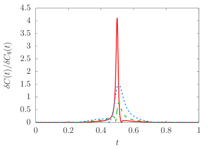
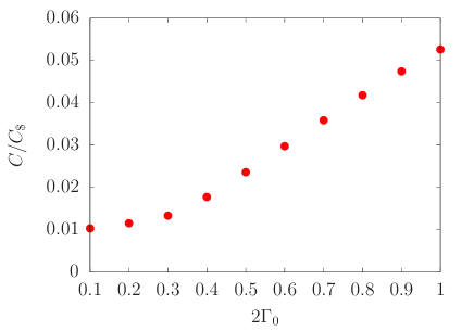
Figure 1: The instantaneous energy cost (left) and the total energy cost (right) against the standard counterparts. The instantaneous energy cost is plotted with respect to time for the energy gap $2\Gamma_{0}=0.2$ (red solid curve), $0.4$ (green dashed curve), and $0.8$ (blue dotted curve), and the total energy cost is plotted with respect to the size of the energy gap (red circles).

Here, the instantaneous energy cost is plotted for $2\Gamma_{0}=0.2$, $0.4$, and $0.8$, and the total energy cost is plotted for $2\Gamma_{0}=0.1,0.2,\dots,1$. We notice that general fast-forward scaling with phase (12) significantly suppress the instantaneous energy cost except for the vicinity of the energy gap. We also find that the total energy cost is significantly suppressed.

We will additionally consider (sub)optimization of the second term to suppress the instantaneous energy cost in the vicinity of the energy gap. It can achieved when

$$f_{+}(T_{\mathrm{FF}}/2)-f_{-}(T_{\mathrm{FF}}/2)=2\pi k,$$ (36)

with an integer $k$. To satisfy this condition, we modulate the phase (12) as

$$\frac{df_{\sigma}(t)}{dt}=\sigma(1+\delta)\frac{T}{T_{\mathrm{FF}}}\sqrt{\left(\omega_{0}-\frac{2\omega_{0}t}{T_{\mathrm{FF}}}\right)^{2}+\Gamma_{0}^{2}},$$ (37)

with small $\delta$. Then, the condition (36) says

$$\delta=\frac{1}{T}\frac{4\pi\omega_{0}k}{\omega_{0}\sqrt{\omega_{0}^{2}+\Gamma_{0}^{2}}+\Gamma_{0}^{2}\log\frac{1}{\Gamma_{0}}(\omega_{0}^{2}+\sqrt{\omega_{0}^{2}+\Gamma_{0}^{2}})}-1,$$ (38)

and we notice that it gives $\delta\approx 0.00427$ when $k=4$ in the present parameter setting with $\Gamma_{0}=0.1$. We depict the instantaneous energy cost of fast-forward scaling with this modulation in Fig. 2.

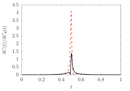
Figure 2: The instantaneous energy cost against the standard instantaneous energy cost. The horizontal axis is time. The black solid curve represents a scheme with modulation $\delta=0.00427$ and the red dashed curve represents that without modulation. Here, the energy gap is $2\Gamma_{0}=0.2$.

We find that the peak in the instantaneous energy cost around the energy gap is suppressed. In this way, we can suppress the both terms in Eq. (32).

We expect that the above lessons hold for general cases where the time-dependent measurement basis is given by the energy-eigenstate basis at rescaled time. Indeed, for a general Hamiltonian

$$\hat{H}(t)=\sum_{n}E_{n}(t)|n(t)\rangle\langle n(t)|,$$ (39)

where $E_{n}(t)$ is the energy eigenvalue and $|n(t)\rangle$ is the corresponding energy eigenstate, the squared Hilbert-Schmidt norm of the fast-forward Hamiltonian is given by

$$\|\hat{H}_{\mathrm{FF}}(t)\|^{2}=\sum_{n}\left(\frac{df_{n}(t)}{dt}-\frac{ds}{dt}E_{n}(s)\right)^{2}+2\left(\frac{ds}{dt}\right)^{2}\sum_{\begin{subarray}{c}m,n\\ (m\neq n)\end{subarray}}\left|\frac{\langle m(s)|\bm{(}\partial_{s}\hat{H}(s)\bm{)}|n(s)\rangle}{E_{n}(s)-E_{m}(s)}\right|^{2}[1-\cos\bm{(}f_{m}(t)-f_{n}(t)\bm{)}].$$ (40)

Here, the coefficient of the second term is the matrix element of the counterdiabatic Hamiltonian. Therefore, optimization of the first term results in the large instantaneous energy cost in the vicinity of the energy gap, but we could mitigate it by slightly modifying the phase. Note that the fast-forward Hamiltonian with the optimization of the first term and without modulation is given by

$$\hat{H}_{\mathrm{FF}}(t)=i\frac{ds}{dt}\sum_{\begin{subarray}{c}m,n\\ (m\neq n)\end{subarray}}\left(1-e^{i\bm{(}f_{m}(t)-f_{n}(t)\bm{)}}\right)|m(s)\rangle\langle m(s)|\partial_{s}n(s)\rangle\langle n(s)|.$$ (41)

VI Summary

In this paper, we introduced the instantaneous and total energy costs of fast-forward scaling, and proposed energy-saving fast-forward scaling as a time-efficient and energy-efficient control method. We applied it to the two-level system and quantum annealing in the Ising spin glass. We also discussed the energy costs of fast-forward scaling in the two-level system with the energy-eigenstate basis. We found that the instantaneous energy cost can significantly be suppressed except for the vicinity of the energy gap. Moreover, we can mitigate the instantaneous energy cost around the energy gap by slightly modulating the phase. Notably, the total energy cost is quite low even without mitigation of the instantaneous energy cost. We believe that the present proposal and future followup enable us to realize energy-efficient quantum technologies.