Considerations on the relaxation time in shear-driven jamming

Abstract

We study the jamming transition in a model of elastic particles under shear at zero temperature, with a focus on the relaxation time $\tau_{1}$. This relaxation time is from two-step simulations where the first step is the ordinary shearing simulation and the second step is the relaxation of the energy after stopping the shearing. $\tau_{1}$ is determined from the final exponential decay of the energy. Such relaxations are done with many different starting configuration generated by a long shearing simulation in which the shear varible $\gamma$ slowly increases. We study the correlations of both $\tau_{1}$, determined from the decay, and the pressure, $p_{1}$, from the starting configurations as a function of the difference in $\gamma$. We find that the correlations of $p_{1}$ are more long lived than the ones of $\tau_{1}$ and find that the reason for this is that the individual $\tau_{1}$ is controlled both by $p_{1}$ of the starting configuration and a random contribution which depends on the relaxation path length—the average distance moved by the particles during the relaxation. We further conclude that it is $\gamma_{\tau}$, determined from the correlations of $\tau_{1}$, which is the relevant one when the aim is to generate data that may be used for determining the critical exponent that characterizes the jamming transition.

I Introduction

In the everyday world there are many examples of disordered systems that change from a flowing state to a rigid state due to a change of some control parameter. The examples are as different as shaving cream and grains in silos. An early suggestion was the existence of the “jamming phase diagram” Liu and Nagel (1998) with the conjecture that the transition from flowing to rigid in disordered systems has the same properties whether the control parameter is density, shear stress, or temperature. It was however later shown that the shear-driven jamming transition, which takes place due to the change in density at zero temperature, is a different phenomenon than equilibrium glassy behavior Ikeda et al. (2012); Olsson and Teitel (2013). Another fundamental insight is that the shear-driven jamming transition of soft particles is perfectly sharp only in the limit of vanishing shear rate Olsson and Teitel (2007).

A path towards a better understanding of these systems is the study of simple models of disorderd collections of particles through computer simulations. A complication is however that the study of zero-temperature processes requires different methods than the ones used in molecular dynamics. In standard molecular dynamics the velocity of the particles automatically makes the system explore phase space and the measurement of different kinds of quantities along this trajectory gives ensemble averages of these quantities. For macroscopic particles of granular matter the thermal velocity is however negligible and ensembles of configurations need to be generated by other means. One way to achieve this is by constantly shearing the system, commonly done with Lees-Edwards boundary conditions Evans and Morriss (1990), which allow for shearing of the system indefinitely with periodic boundaries in all directions.

The shear-driven jamming transition is characterized by the increase of shear viscosity with increasing density and the cleanest behavior is for a system of hard disks. For hard disks the viscosity only depends on the density, $\phi$, and the exponent $\beta$ describes the divergence of the shear viscosity at $\phi_{J}$,

$$\eta_{\mathrm{hd}}(\phi)\sim(\phi_{J}-\phi)^{-\beta}.$$ (1)

A method for simulating with hard particles has been devised and was used in Ref. Lerner et al. (2012). That method is however in practice limited to rather small systems and densities at some distance below jamming. This is so since the method relies on the diagonalization of a matrix, which has to be done each time the contact network changes. Another approach is to simulate soft particles at different shear rates $\dot{\gamma}$—where the limit $\dot{\gamma}\to 0$ corresponds to the hard disk limit—and to try to determine the behavior in that limit by scaling analyses Olsson and Teitel (2007, 2011). Yet another method to approach the hard disk limit—a method of relevance for the present paper—is to start from configurations produced in the shearing simulations, stop the shearing and let the energy relax down towards zero energy. (Similar relaxations were first done in Ref. Hatano (2009).) The final part of this relaxation turns out to be exponential to an excellent approximation and each relaxation gives a relaxation time $\tau_{1}$. We here use a notation where $\tau_{1}$, $z_{1}$, and $p_{1}$ denote quantities from single configurations or relaxations, whereas $\tau$, $z$, and $p$ denote averages over many configurations. From the configurations we also determine $z_{1}$ which is the average number of contacts per particle in the final configuration, after the rattlers have been removed. (The rattlers are the particles with $\leq D$ contacts which do not contribute to the stability of the network.) It is then found that $\tau_{1}$ is directly related to the distance to isostaticity, given by $\delta z_{1}\equiv z_{c}-z_{1}$ Olsson (2015a), with $z_{c}=2d$ Alexander (1998). (See Ref. Goodrich et al. (2012) for the generalization of this expression to finite $N$). The relaxation time is algebraically related to the distance to isostaticity, $\tau_{1}\sim\delta z_{1}^{-\beta/u_{z}}$ Olsson (2015a). Here $z_{c}-z\sim(\phi_{J}-\phi)^{u_{z}}$ and it is commonly believed that $u_{z}=1$ Heussinger and Barrat (2009).

We also remark that it has been claimed Nishikawa et al. (2021) that the determinations of $\tau_{1}$ suffer from a problematic finite size dependence which in effect invalidates the method. As discussed in Appendix A other studies confirm this finite size effect but show that it is a serious problem only for certain cases and that it does not pose a problem for the simulations as in Ref. Olsson (2015a).

The determination of the relaxation time by starting from configurations obtained through steady shearing Olsson (2015a) is therefore a method that gives results relevant for the hard disk limit, that may be used for simple and clean determinations of the critical behavior. The question however remains on how to perform such analyses efficiently and the original motivation behind the present work was to find guidelines for such more efficient simulations. These investigations did however lead to a number of interesting findings both on the workings of the relaxation simulations and for the shear-driven simulations which means that these findings are the central results whereas the quest for an optimal approach in the simulations becomes secondary.

When approaching close to $\phi_{J}$ one would better make use of big system sizes both to avoid the spurious jamming that can happen in smaller systems and to get a smaller spread in the obtained $\tau_{1}$ Olsson (2015a). It is also desirable to perform the initial shearing simulations with small shear strain rates, since that somewhat speeds up the ensuing relaxations. The question is then how to chose the distance in terms of shear strain, $\gamma$, between successive starting configurations. The desire is to avoid getting relaxations that are strongly correlated to each other and at the same time avoid wasting simulation time on unnecessarily long shearing simulations between the successive relaxations.

Beside the practical questions there are also questions on the workings of the relaxations and one such question is the connection between the properties of the starting configuration and the relaxed configuration. Specifically we ask to what extent it is possible to predict $\tau_{1}$ from the pressure $p_{1}$ of the starting configuration. The answer to this question is important both for the above stated question on the efficient use of simulations and for a better understanding of the dynamics at densities below jamming.

The organization of the manuscript is as follows: In Sec. II we describe the model and the simulations and also the scaling assumptions and the analyses employed in this work. In Sec. III we start by first examining the correlations of relaxation times $\tau_{1}$ generated from configurations a distance $\gamma$ apart. Because of the difficulty in getting good statistics for that quantity we examine to what extent it is possible to predict $\tau_{1}$ from the pressure of the starting configuration, $p_{1}$, and find that $\tau_{1}$ is governed both by $p_{1}$ and by a random term which is related to the real space distance between the relaxed configuration and its starting configuration. We then also examine the pressure correlations and find a rich behavior, but also show that the behavior may be understood in terms of the scaling approach. In Sec. IV we discuss the implications of the findings for efficient simulations with the aim of high-precision determinations of a critical exponent. In Sec. V we give a short summary of the findings. We also include an appendix which discusses the possibility of logarithmic corrections to scaling that—if present—could make the determination of the critical divergence exceedingly difficult, and has been put forward as the reason for the discrepancy between numerically determined exponents Olsson and Teitel (2011); Olsson (2015b); Kawasaki et al. (2015) and the ones obtained from a certain theoretical approach DeGiuli et al. (2015); Ikeda (2020).

II Model, simulations, and analyses

II.1 Simulation model

For the simulations we follow O’Hern et al. O’Hern et al. (2003) and use a simple model of bi-disperse frictionless disks in two dimensions with equal numbers of particles with two different radii in the ratio 1.4. We use Lees-Edwards boundary conditions Evans and Morriss (1990) to introduce a time-dependent shear strain $\gamma=t\dot{\gamma}$. We take $r_{ij}$ for the distance between the centers of two particles and $d_{ij}$ for the sum of their radii. The relative overlap then becomes $\delta_{ij}=1-r_{ij}/d_{ij}$. The interaction between two overlapping particles is $V_{p}(r_{ij})=\epsilon\delta_{ij}^{2}/2$; we take $\epsilon=1$. The force on particle $i$ from particle $j$ is $\mathbf{f}^{\mathrm{el}}_{ij}=-\nabla_{i}V_{p}(r_{ij})$, which means that the magnitude becomes $f^{\mathrm{el}}_{ij}=\epsilon\delta_{ij}/d_{ij}$. The simulations are performed at zero temperature. Length is measured in units of the diameter of the small particles, $d_{s}$.

The total interaction force on particle $i$ is $\mathbf{f}^{\mathrm{el}}_{i}=\sum_{j}\mathbf{f}^{\mathrm{el}}_{ij}$, where the sum extends over all particles $j$ in contact with $i$. The simulations have been done with the RD₀ (reservoir dissipation) model Vågberg et al. (2014) with the dissipating force $\mathbf{f}^{\mathrm{dis}}_{i}=-k_{d}\mathbf{v}_{i}$ where $\mathbf{v}_{i}\equiv d\mathbf{r}_{i}/dt-y_{i}\dot{\gamma}\hat{x}$ is the non-affine velocity, i.e. the velocity with respect to a uniformly shearing velocity field, $y_{i}\dot{\gamma}\hat{x}$. In the overdamped limit the equation of motion is $\mathbf{f}^{\mathrm{el}}_{i}+\mathbf{f}^{\mathrm{dis}}_{i}=0$ which becomes $\mathbf{v}_{i}=\mathbf{f}^{\mathrm{el}}_{i}/k_{d}$. We take $k_{d}=1$ and the time unit $\tau_{0}=d_{s}^{2}k_{d}/\epsilon=1$. The equations of motion were integrated with the Heuns method with time step $\Delta t/\tau_{0}=0.2$.

Many quantities were measured during the shearing simulations. Two examples of relevance for the present work are pressure $p$, and the average magnitude of the non-affine particle velocity $v=\left<|\mathbf{v}_{i}|\right>$. We will below refer to earlier analyses of $p$ in Ref. Olsson and Teitel (2011). The properties of $v$ have been discussed in Ref. Olsson (2016); we here just note that different powers of $v$ scale differently as criticality is approached, such that $\left<\mathbf{v}_{i}^{2}\right>$ and $\left<|\mathbf{v}_{i}|\right>^{2}$ diverge differently.

II.2 Scaling relations

Shear-driven jamming has been found to be a critical phenomenon with shear strain rate one of the relevant parameters, which means that jamming transition takes place at $(\phi,\dot{\gamma})=(\phi_{J},0)$ and that many properties are expected to scale with the distance to jamming. A general review of scaling may be found in Ref. Vågberg et al. (2016). With $\delta\phi=\phi-\phi_{J}$ the pressure is expected to scale as

$$p(\delta\phi,\dot{\gamma})=b^{-y/\nu}\tilde{g}(\delta\phi\,b^{1/\nu},\dot{\gamma}b^{z}).$$ (2)

where $\nu$ is the correlation length exponent, $z$ is the dynamical critical exponent, and $y$ is the scaling dimension of $p$. It should be noted that this expression neglects the correction to scaling term Olsson and Teitel (2011) which is important for precise analyses close to jamming and has gotten a new interpretation in recent works Olsson (2022a, 2023).

With $b=\dot{\gamma}^{-1/z}$ and the notation $q=y/z\nu$ this becomes Olsson and Teitel (2007)

$$p(\phi,\dot{\gamma})=\dot{\gamma}^{q}g\left(\frac{\phi-\phi_{J}}{\dot{\gamma}^{1/z\nu}}\right).$$ (3)

To describe the deviations from the hard disk limit we note that the pressure is one of many quantities which is $\propto\dot{\gamma}$ in the $\dot{\gamma}\to 0$ limit. For $\eta_{p}\equiv p/\dot{\gamma}$ Eq. (2) translates to

$$\eta_{p}(\delta\phi,\dot{\gamma})=b^{z-y/\nu}\tilde{h}_{\eta}(\delta\phi\,b^{1/\nu},\dot{\gamma}b^{z}),$$ (4)

and $(\phi_{J}-\phi)b^{1/\nu}=1$ gives $b=(\phi_{J}-\phi)^{-\nu}$ which in turn leads to

$$\eta_{p}(\phi,\dot{\gamma})=(\phi_{J}-\phi)^{-\beta}h_{\eta}\left(\frac{\dot{\gamma}}{(\phi_{J}-\phi)^{z\nu}}\right),$$ (5)

where $\beta=z\nu-y$.

The present work focuses on the relaxation time $\tau$ which, in the hard disk limit, behaves the same as $\eta_{p}$ Olsson (2015b); Lerner et al. (2012),

$$\tau(\phi,\dot{\gamma})=A_{\tau}(\phi_{J}-\phi)^{-\beta},\quad\dot{\gamma}\to 0.$$ (6)

Another quantity of interest is the velocity per unit of shear strain which diverges as Olsson (2016)

$$\lim_{\dot{\gamma}\to 0}v(\phi,\dot{\gamma})/\dot{\gamma}=A_{v}(\phi_{J}-\phi)^{-u_{v}},\quad\dot{\gamma}\to 0,$$ (7)

with $u_{v}\approx 1.1$. For finite $\dot{\gamma}$ these expressions may be generalized through the same kind of relations,

$$\tau(\phi,\dot{\gamma})\sim(\phi_{J}-\phi)^{-\beta}h_{\tau}\left(\frac{\dot{\gamma}}{(\phi_{J}-\phi)^{z\nu}}\right),$$ (8)

$$v(\phi,\dot{\gamma})/\dot{\gamma}\sim(\phi_{J}-\phi)^{-u_{v}}h_{v}\left(\frac{\dot{\gamma}}{(\phi_{J}-\phi)^{z\nu}}\right).$$ (9)

Note however the different nature of these quantities. The determination of the relaxation time is from two-step simulations that are done by first shearing at a certain shear strain rate and then stop the shearing and let the system relax to zero energy. The non-affine velocity per shear rate, $v(\phi,\dot{\gamma})/\dot{\gamma}$, characterizes the flowing sheared steady state, whereas the relaxation time, $\tau$, is from the final stage of this relaxation.

II.3 Analyses

To determine the relaxation time we run simulations as described above at zero temperature and fixed $\gamma$ (i.e. with $\dot{\gamma}=0$) which leads to an energy decreasing towards zero; the simulations are aborted when the energy per particle is $E<10^{-20}$. The relaxation time is then determined from the exponential decay of the energy per particle by fitting $E(t)$ to

$$E(t)\sim e^{-t/\tau_{1}},\quad E(t)<10^{-17}.$$ (10)

For each parameter set, $N$, $\phi$, and $\dot{\gamma}$, the starting configurations are from a long shearing simulation that gives a large number of different starting configurations with different $\gamma$. The relaxation simulations then give a set of relaxation times, $\tau_{1}(\gamma)$. (The individual determinations are denoted by $\tau_{1}$ whereas their average is denoted by $\tau$.) On general grounds one expects two starting configurations that differ only by a small shear $\gamma$ to be similar and to also lead to similar relaxation times and one of the goals of the present work is to examine how quickly this similarity decays and thus to determine the correlation shear—which is the analogous of the correlation time—for $\tau_{1}$.

The autocorrelation function of some quantity $A$ is a measure of the correlations in the fluctuations of $A$, i.e. $\delta A=A-\left<A\right>$. The autocorrelation function is then $\left<\delta A(t^{\prime})\delta A(t^{\prime}+t)\right>$, where the average is over different initial times $t^{\prime}$. When comparing systems that are sheared at different shear strain rates there is a trivial shear strain rate dependence and it is therefore convenient to instead express the correlation function in terms of the change in the shearing variable, $\gamma$,

$$\rho_{A}(\gamma)=\frac{\left<\delta A(\gamma^{\prime}+\gamma)\delta A(\gamma^{\prime})\right>}{\left<(\delta A)^{2}\right>}.$$ (11)

We will examine this correlation function for two different quantities, $A=1/\tau_{1}$ and $A=p$ and beside some results extracted from these correlation functions we will be able to draw some conclusions about the relaxation processes.

III Results

III.1 Correlations of relaxation times

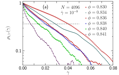
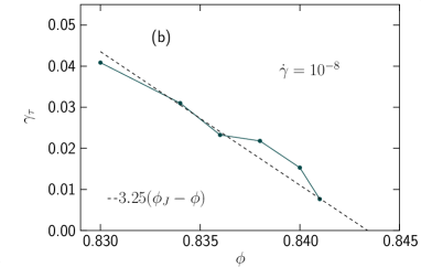
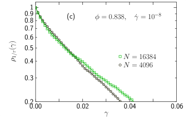
Figure 1: Correlation function for from the inverse relaxation time. Panel (a) is the correlation function $\rho_{1/\tau}(\gamma)$ obtained with $N=4096$ particles, shear strain rate $\dot{\gamma}=10^{-8}$, at densities $\phi=0.830$ through 0.841. The correlation shear, $\gamma_{\tau}$, is defined to be the value of $\gamma$ for which the correlation function is $\rho_{1/\tau}=e^{-1}$. Panel (b) which is $\gamma_{\tau}$ vs $\phi$, shows that $\gamma_{\tau}$ decreases as $\phi_{J}$ is approached from below in an approximately linear way, $\gamma_{\tau}\sim\phi_{J}-\phi$. Panel (c) which shows $\rho_{1/\tau}(\gamma)$ for two different system sizes, $N=4096$ and $N=16384$, illustrates that the correlation function is independent of $N$.

To analyze correlations of $\tau_{1}$ we determine $\rho_{1/\tau}(\gamma)$ from Eq. (11) with $A=1/\tau_{1}$ for $\dot{\gamma}=10^{-8}$ and $N=4096$ particles and at densities $\phi=0.830$ through 0.841, closely below $\phi_{J}\approx 0.8434$. The rationale for determining the correlations of $1/\tau_{1}$ instead of $\tau_{1}$ is that $\tau_{1}$ can occasionally be very big which could mean that a few big values would dominate the correlation function. This problem is not present when instead determining the correlation of $1/\tau_{1}$.

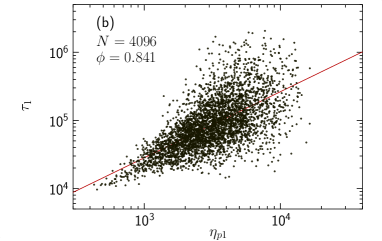
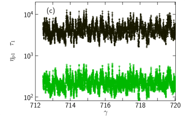
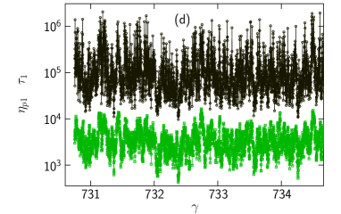
Figure 2: Plots of $\tau_{1}$ and $\eta_{p1}$ at two different densities, $\phi=0.836$ and 0.841. Here $\eta_{p1}$ are from the starting configurations whereas $\tau_{1}$ are from the relaxations. The question is to what extent $\tau_{1}$ from the relaxation may be predicted from $\eta_{p1}\equiv p_{1}/\dot{\gamma}$ of the starting configuration. The data are for $N=4096$ particles and shear rate $\dot{\gamma}=10^{-8}$ for the shearing simulations. Panels (a) and be which show $\tau_{1}$ vs $\eta_{p1}$ shows that these quantities are strongly correlated for the lower density $\phi=0.836$ and more weakly correlated at $\phi=0.841$. The lower panels are the same data but now plotted vs $\gamma$ ($\sim$ simulation time). Panel (c) is for $\phi=0.836$ whereas panel (d) is for $\phi=0.841$. In both cases we find that $\tau_{1}$ closely follows $\eta_{p1}$—the minima and maxima of $\eta_{p1}$ are closely followed by similar minima and maxima in $\tau_{1}$—but also that the spread is bigger in panel (d) which is for the higher $\phi$.

Fig. 1(a) shows $\rho_{1/\tau}(\gamma)$. We find that each curve to a decent approximation shows an exponential decay and that the slope of the curves increase as $\phi$ increases towards $\phi_{J}$. To determine the correlation shear—the analogous quantity to the correlation time—one should ideally fit the tail of $\rho_{1/\tau}(\gamma)$ to an exponential decay, but since our data are rather noisy this isn’t feasible and we therefore instead determine the correlation shear $\gamma_{\tau}$ from the shear strain that gives $\rho_{1/\tau}(\gamma_{\tau})=e^{-1}$, i.e. from the crossings of the horizontal dashed line in Fig. 1(a). Fig. 1(b) shows $\gamma_{\tau}$ vs $\phi$ and we note that the figure can be taken to suggest a linear behavior, $\gamma_{\tau}\propto\phi_{J}-\phi$.

The data above are determined with $N=4096$ and an interesting and non-trivial question is on the finite size dependence of $\gamma_{\tau}$. One possibility would be that a larger number of particles would give more places with important changes of the contact pattern which would lead to a bigger change in $\tau_{1}$ for each change in $\gamma$. Our results do however suggest that there is no real finite size dependence for our quite big systems. (For sufficiently small $N$ one would however expect changes of all kinds of quantities.) This is illustrated by Fig. 1(c) which shows $\rho_{1/\tau}(\gamma)$ for $N=4096$, 16384 particles, determined with $\phi=0.838$ and $\dot{\gamma}=10^{-8}$.

Fig. 1(b) is for a single shear strain rate, $\dot{\gamma}=10^{-8}$, and a further question is on the dependence of $\gamma_{\tau}$ on the shear strain rate. To that end we have attempted the same kind of analyses for different shear strain rates but found the data to be somewhat too noisy for any safe conclusions. The basic problem is that the determinations of $\rho_{1/\tau}(\gamma)$ requires a large number relaxation times, $\tau_{1}$, which are obtained through time consuming relaxations of the system to (almost) vanishing energy. With a limited number of such $\tau_{1}$ the correlation function $\rho_{1/\tau}(\gamma)$ for different $\phi$ become quite noisy which makes it difficult to achieve precise determinations of $\gamma_{\tau}$.

As an alternative route to more insight we have therefore turned to other analyses. The approach is based on the expectation that the individual $\tau_{1}$ should be strongly influenced by properties—as e.g. the pressure—of the respective initial configurations, and that the correlations between such quantities should be much easier to determine since there are considerably more available data. For such an initial property we here make use of the pressure, and the approach is therefore to first turn to a comparison between relaxation time and the pressure of the corresponding initial configuration, and then, as a second step, examine these pressure correlations. As we will see these correlations turn out to be somewhat different and do not directly help answer our questions. This approach does nevertheless lead to some unexpected new insights.

III.2 Relaxation time and pressure

To examine the relation between $\tau_{1}$, determined from the last stage of the relaxation, and $\eta_{p1}\equiv p_{1}/\dot{\gamma}$, from the initial configurations (before the relaxation), Fig. 2 shows $\tau_{1}$ and $\eta_{p1}$ for $\dot{\gamma}=10^{-8}$ and $N=4096$, at two different densities, $\phi=0.836$ and 0.841. Fig. 2(a) which is $\tau_{1}$ vs $\eta_{p1}$ for $\phi=0.836$ shows that these data are strongly correlated whereas Fig. 2(b), obtained at the higher density $\phi=0.841$, gives evidence for a weaker correlation. Panels (c) and (d) show the same data but now plotted vs $\gamma$. For the lower $\phi$ in Fig. 2(c) it is clear that the two quantities follow each other closely but Fig. 2(d), which displays the same kind of data for the higher $\phi=0.841$, shows that the minima and the maxima of $\eta_{p1}$ are reflected in $\tau_{1}$, but that there is also a big fluctuating random component to $\tau_{1}$.

To quantify this fluctuating factor we introduce

$$f_{1}=\ln\frac{\tau_{1}}{\eta_{p1}},$$ (12)

which is from the ratio of the pressure of the initial configuration and the relaxation rate determine from relaxation simulations. The rational for taking the logarithm is, as shown in Fig. 3(a) and (b), that the distribution of $\tau_{1}/\eta_{p1}$ is strongly skewed whereas the distribution of the logarithm of the same quantity is similar to a Gaussian distribution, as if $f_{1}$ were the sum of a number of independent random variables.

If $\tau_{1}$ were exactly predicted by $\eta_{p1}$ $f_{1}$ would be a constant and to quantity the spread in $f_{1}$ we determine

$$\mathrm{sdev}[f_{1}]=\sqrt{\left<f_{1}^{2}\right>-\left<f_{1}\right>^{2}},$$

which is then a measure of the size of the random fluctuating factor. Fig. 3(c) which is $\mathrm{sdev}[f_{1}]$ vs $\phi$ for two different sizes, $N=4096$, 16384, shows that this quantity is small at low $\phi$ and increases rapidly with increasing $\phi$. Further analyses (see below) suggest that $\mathrm{sdev}[f_{1}]\sim 1/\sqrt{N}$, just as expected from elementary statistics of $N$ independent values.

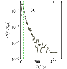
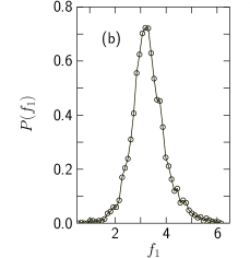
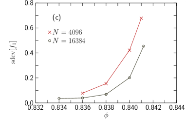
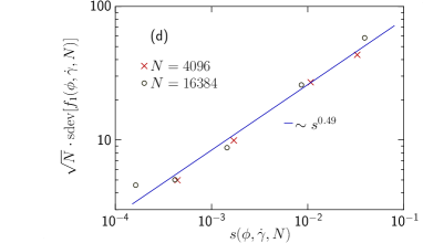
Figure 3: Properties of $f_{1}\equiv\ln(\tau_{1}/\eta_{p1})$. All data are for $\dot{\gamma}=10^{-8}$. Panels (a) and (b) show that the distribution of $\tau_{1}/\eta_{p1}$ is strongly skewed whereas the distribution of $f_{1}\equiv\ln(\tau_{1}/\eta_{p1})$ is similar to a Gaussian distribution. This is taken to suggest that $f_{1}$ is a reasonable quantity for analyses. Panel (c) shows the spread in $f_{1}$—denoted by $\mathrm{sdev}[f_{1}]$—vs $\phi$ for two different sizes, $N=4096$ and 16384. The finite size dependence is to a good approximation given by $\sim 1/\sqrt{N}$. Panel (d) shows the same data versus $s$, which is the average displacement during the relaxation, now compensated for the $\sqrt{N}$ dependence. A fit gives $\sqrt{N}\;\mathrm{sdev}[f_{1}]\sim s^{0.49}$, which suggests a dependence $\sim\sqrt{s}$. The conclusion is that each small $\Delta s$ from the relaxation contributes a random constant to $f_{1}$ and thus a random factor to $\tau_{1}/\eta_{p1}$.

The reason for the strong correlation between $\eta_{p1}$ and $\tau_{1}$ at the lower densities is that the each final configuration is very close to its corresponding initial configuration. Conversely, the bigger fluctuations of $f_{1}$ at higher densities suggests the that the properties of the system often change a lot during the relaxations. As a measure of the distance between initial and final configurations in ordinary space, we introduce the relaxation path length which is the average distance moved by the particles during the relaxation,

$$s(\phi,\dot{\gamma},N)=\left<\int_{0}^{\infty}|\mathbf{v_{i}}(t)|dt\right>.$$

The average is here over both particles and relaxation runs performed with the same parameters, $\phi$, $\dot{\gamma}$, and $N$.

Figure 3(d) is a parametric plot of $\mathrm{sdev}[f_{1}(\phi,\dot{\gamma},N)]$ vs $s(\phi,\dot{\gamma},N)$ for two system sizes, $N=4096$, $16384$, shear strain rate $\dot{\gamma}=10^{-8}$, and densities $\phi=0.834$ through $0.8412$. The system size dependence found in Fig. 3(c) is here taken care of through a factor of $\sqrt{N}$ and the plotted quantity is thus $\sqrt{N}\cdot\mathrm{sdev}[f_{1}(\phi,\dot{\gamma},N)]$. The fit to an algebraic dependence on $s(\phi,\dot{\gamma},N)$ gives the exponent 0.49 which suggests

$$\mathrm{sdev}[f_{1}(\phi,\dot{\gamma},N)]\sim\frac{\sqrt{s(\phi,\dot{\gamma},N)}}{\sqrt{N}}.$$ (13)

We note that this is consistent with elementary statistics if one considers $f_{1}$ to be the average of $N$ different terms which each is the sum of $\propto s$ different terms. The logarithm in the definition of $f_{1}$ lets us conclude that each small $\Delta s$ contributes a random factor to $\tau_{1}$.

To summarize this part we have found that $\tau_{1}$ is directly controlled by $\eta_{p1}$ at low densities and that the behavior at higher $\phi$ is similar but with big random fluctuations. We have also found that the size of this random contribution to $\tau_{1}$ is directly related to the average distance moved by the particles during the relaxation.

III.3 Pressure correlations

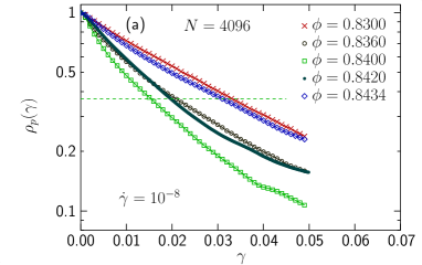
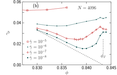
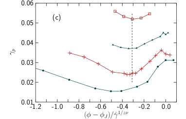
Figure 4: Correlation shear, $\gamma_{p}$, determined from $p_{1}(\gamma)$ measured in the shearing simulation. Panel (a) shows $\rho_{p}(\gamma)$ for $N=4096$ particles, shear strain rate $\dot{\gamma}=10^{-8}$, and densities $\phi=0.830$ through 0.840. (Data for more densities are excluded in order not to clutter the figure.) The correlation shear, $\gamma_{p}$, is determined as the $\gamma$ for which $\rho_{p}(\gamma)=e^{-1}$. Panel (b) which is the correlation shear, $\gamma_{p}$ vs $\phi$ for three different $\dot{\gamma}$, shows a clear dependence on $\dot{\gamma}$. For each $\dot{\gamma}$ there is a minimum at a certain $\phi_{\mathrm{min}}(\dot{\gamma})$. As $\dot{\gamma}$ decreases the position of this minimim moves towards $\phi_{J}$. Panel (c) The same data but plotted vs the scaled distance from jamming as suggested by Eq. (3). We note that the minima of the respective curves are on top of each other, except for the data for the lowest $\dot{\gamma}$. This deviation is tentatively attributed to a finite size effect that appears as the system size becomes comparable to the correlation length.

We then turn the correlations of pressure with the aim to get an understanding of the size of the shear strain, $\gamma_{p}$, that characterizes the decay of the pressure correlations in shear-driven simulations.

Figure 4(a) shows the correlation function $\rho_{p}(\gamma)$ for $N=4096$ particles, shear strain rate $\dot{\gamma}=10^{-8}$, and densities $\phi=0.830$ through 0.8434. We find that $\rho_{p}(\gamma)$ decays exponentially for each $\phi$, and determine the correlation shear $\gamma_{p}$ from the condition $\rho_{p}(\gamma_{p})=e^{-1}$. Fig. 4(b) shows $\gamma_{p}$ vs $\phi$ for different $\dot{\gamma}$. The solid dots are from the data in Figure 4(a), the other symbols are for three higher shear strain rates.

We note that the behavior of $\gamma_{p}(\phi)$ as $\dot{\gamma}\to 0$ suggest that $\gamma_{p}(\phi)$ in the hard disk limit goes approximately linearly to zero, as shown by the dashed line. This is the same kind of behavior as shown for $\gamma_{\tau}$ in Fig. 1(b) and it is also consistent with the finding that a characteristic shear determined from the velocity-velocity correlation at $\phi_{J}$ vanishes as $\dot{\gamma}\to 0$ Olsson (2010). This is also directly related to the fact that $v/\dot{\gamma}$—the distance traveled per unit shear— increases as jamming is approached.

Another interesting observation from Fig. 4(b) is that this correlation shear, for each finite shear strain rate, $\dot{\gamma}$, depends non-monotonously on $\phi$. For each constant shear strain rate the correlation shear, $\gamma_{p}$, first decreases towards a minimum and then increases again when $\phi$ approaches $\phi_{J}$ from below. We will now first relate this behavior to ideas from scaling, then discuss the physical mechanisms behind this decrease and finally consider the change to an increasing trend of $\gamma_{p}$ vs $\phi$.

From the scaling assumption in Eq. (3) follows that the behavior should be controlled by the combination $(\phi-\phi_{J})/\dot{\gamma}^{1/z\nu}$. To test this expectation we plot $\gamma_{p}$ vs $(\phi-\phi_{J})/\dot{\gamma}^{1/z\nu}$ in Fig. 4(c) and we then find that the upward turns, to a decent approximation, take place at a constant $(\phi_{J}-\phi)/\dot{\gamma}^{1/z\nu}$. There is a deviation from that behavior for the smallest shear strain rate, $\dot{\gamma}=10^{-8}$, and we attribute this to a finite size effect which could be visible when the correlation length, which increases as $\phi_{J}$ is approached from belowOlsson and Teitel (2020), becomes comparable to the system size.

Turning to the physical reason for the decrease of $\gamma_{p}$ with increasing $\phi$, at low $\phi$, we believe that this is an effect of the increasing particle velocity as $\phi\to\phi_{J}$, described by Eq. (7). The reasoning is that we expect two configurations that are generated by the shearing dynamics should be substantially different—such that their respective $p_{1}$ are also different—if the particles have on average moved a certain characteristic distance, $\ell$. This gives the time scale $t_{v}=\ell/v$ and $\gamma_{p}=t_{v}\dot{\gamma}=\ell\dot{\gamma}/v$, which together with Eq. (7) for the divergence of $v/\dot{\gamma}$ becomes $\gamma_{p}=(\ell/A_{v})(\phi_{J}-\phi)^{u_{v}}$. The dashed line in Fig. 4(b) is an approximate description of the behavior in the $\dot{\gamma}\to 0$ limit, assuming $u_{v}=1$. The rectilinear behavior shown there is in reasonable agreement with the behavior described by the exponent $u_{v}\approx 1.1$.

We now turn to the change in trend of $\gamma_{p}(\phi)$ and we are going to argue that it goes together with a change from hard to soft particles—i.e. a change from negligible to a finite particle overlaps. When the shearing is sufficiently slow that the system has time to relax down to very small particle overlaps the system is in the hard particle limit. Since the energy relaxation is governed by the relaxation time, $\tau$, the system should be close to the hard disk limit as long as the relaxation time is smaller than all other relevant time scales. With the velocity time scale, $t_{v}=\ell/v$, introduced above, we get the criterion $\tau\ll t_{v}$, and the expectation of a change of trend when that condition is no longer fulfilled.

We now argue that the change in behavior when $t_{v}\approx\tau$ is consistent with the expectation from scaling discussed above, that the behavior should depend on the combination $(\phi-\phi_{J})/\dot{\gamma}^{1/z\nu}$. For this comparison we first make use of the relation $z\nu=\beta+y$ Olsson and Teitel (2011) to rewrite the scaling variable as

$$\frac{\phi-\phi_{J}}{\dot{\gamma}^{1/(\beta+y)}}.$$ (14)

From Eq. (7) we then find

$$t_{v}=\frac{\ell}{A_{v}\dot{\gamma}}(\phi_{J}-\phi)^{u_{v}},$$ (15)

which together with Eq. (6) and the criterion $\tau\ll t_{v}$ gives

$$A_{\tau}(\phi_{J}-\phi)^{-\beta}\ll\frac{\ell}{A_{v}\dot{\gamma}}(\phi_{J}-\phi)^{u_{v}},$$ (16)

which implies that the criterion for being in the hard disk limit becomes

$$\frac{\phi_{J}-\phi}{\dot{\gamma}^{1/(\beta+u_{v})}}\gg\mathrm{const}.$$ (17)

This is similar to Eq. (14) and also leads to the suggestion $u_{v}=y$. We also note that the possibility that these two different exponents actually are the same is in agreement with the numerical values in the literature, $y=1.08\pm 0.03$ Olsson and Teitel (2011) and $u_{v}\approx 1.10$ Olsson (2016).

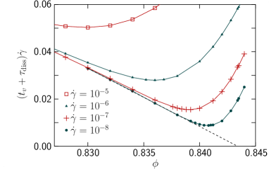
Figure 5: Attempt to predict $\gamma_{p}$ from our two time scales. The time scales are $t_{v}=\ell/v$ from the average particle velocity and the dissipation time $\tau_{\mathrm{diss}}$, from the initial decay of energy in a relaxation, but determined from properties measured in the shearing simulations and given by Eq. (18). Though the agreement with $\gamma_{p}$ in Fig. 4(b) is by no means perfect, we note that this quantity has the same general behavior.

We now also take this one step further and try to approximately express $\gamma_{p}$ in terms of $\tau$ and $t_{v}$. Since $\tau$ is the time scale needed to relax energy or pressure when shearing has been stopped, it is not unreasonable to expect $\tau$ to affect the pressure relaxations also in the presence of shearing. However, since the conditions are so different it follows that a possible relation between $\tau$ and the pressure correlations could at most be an approximative one, only.

In the following, we will make use of a related but different time scale—the dissipation time, $\tau_{\mathrm{diss}}$, described in Ref. Olsson (2015b). This time scale is determined from the initial decay of a relaxation in contrast to $\tau$ which is determined from the final part of the relaxation. These two time scales—$\tau$ and $\tau_{\mathrm{diss}}$—behave the same in the $\dot{\gamma}\to 0$ limit but have the opposite dependence on $\dot{\gamma}$ Olsson (2015b). The decisive advantage with $\tau_{\mathrm{diss}}$ before $\tau$ is however that it may be determined directly from the properties (energy and shear stress) of the shearing simulations Olsson (2015b),

$$\tau_{\mathrm{diss}}=2\frac{E}{\sigma\dot{\gamma}},$$ (18)

without the need for any relaxation steps.

Figure 5 shows the simplest possible way to include the effect of these two different time scales, which is to assume that the effective correlation time is obtained by adding together contributions from these two time scales, such that the correlation shear is given by $\gamma_{p}=(t_{v}+\tau_{\mathrm{diss}})\dot{\gamma}=(\ell/v+\tau_{\mathrm{diss}})\dot{\gamma}$. Here $v$ is the measured average velocity, $\tau_{\mathrm{diss}}$ is from Eq. (18) and the free parameters are $\ell=0.1$, and the prefactor of $\tau_{\mathrm{diss}}$ which we take to be equal to unity. Though the agreement is by no means perfect we note that the curves in Figure 5 capture the general behavior of the simulation data in Figure 4(b). The conclusion is thus that the non-monotonic behavior of $\gamma_{p}$ is an effect of the increase of $\tau$ as $\phi$ approaches $\phi_{J}$ from below.

IV Discussion

IV.1 Comparing the different correlation functions

In the above sections we examined correlations from two different “time” series, $\tau_{1}(\gamma)$ and $p_{1}(\gamma)$ and determined the related $\gamma_{\tau}$ and $\gamma_{p}$. Since the determinations of a large numbers of $\tau_{1}$ are quite computationally demanding the idea was to extract the same kind of information from $p_{1}$ of the initial configurations which would thus reduce the need for a large number of relaxation runs.

Fig. 1 suggests that $\gamma_{\tau}$ from the $\gamma$ dependence of $\tau_{1}$ vanishes approximately linearly as $\phi_{J}$ is approached from below whereas Fig. 4 shows that $\gamma_{p}$ has minima that depend on $\dot{\gamma}$ and move towards $\phi_{J}$ as $\dot{\gamma}$ decreases. To explain the difference in behavior we then noted that there are two contributions to $\tau_{1}$. The first is related to the values of $p_{1}$, and thereby $\eta_{p1}$, in the initial configuration and the second is due to the relaxation processes. The first contribution changes slowly whereas the second component fluctuates much more rapidly and it appears that it is this second component that is responsible for the continued decay of the correlations in Fig. 1(b) when $\gamma_{p}$ from the pressure correlations in Fig. 4(c) turn upwards.

These conclusions appear to be true when $\gamma_{\tau}$ and $\gamma_{p}$ are determined as the values of $\gamma$ that make the correlation functions equal to some given constant, here taken to be $e^{-1}$. The correlations that are visible in the pressure correlations ought however to be present also in $\rho_{1/\tau}(\gamma)$ and should be visible if one were able to access the tail of $\rho_{1/\tau}$ with sufficient precision. To see this we may consider an interval in $\gamma$ where $p_{1}$ is almost a constant. In this range of $\gamma$ $\tau_{1}$ will vary around a certain average that depends on the average $p$. For a different interval in $\gamma$ with another average $p$, $\tau_{1}$ will fluctuate around another average value. From this consideration it appears that correlations that are seen in $p_{1}$ should also be present in $\tau_{1}$. Since the fluctuations in $p_{1}$ are quite small compared to the fluctuations in $\tau_{1}$ it does however seem that it would be virtually impossible to verify the existence of these correlations in $\tau_{1}$.

The question is now what to conclude for efficient relaxation simulations, and what should reasonably be the distance in terms of $\gamma$ between successive starting configurations. It then appears that the answer—as is often the case—depends on what the obtained data should be used for. If the goal is to get statistically independent values $\tau_{1}$ for given $\phi$ and $\dot{\gamma}$ it is reasonable to consider the correlations of the initial configurations and it could then be reasonable to do the relaxation runs by starting at points with the separation $\gamma\gg\gamma_{p}$. If, on the other hand, the goal is to get a set of points ($\tau_{1}$, $\delta z_{1}$) for determining the exponent $\beta/u_{z}$ from $\tau_{1}\sim(\delta z_{1})^{-\beta/u_{z}}$, then a possible bias of these points towards high or small values of $\tau_{1}$ and $\delta z_{1}$ would not be a problem, and one could then well make use of starting configurations that are quite close together in $\gamma$, but still with $\gamma\gg\gamma_{\tau}$ where $\gamma_{\tau}$ is from the apparent correlations of $1/\tau$.

IV.2 Implications for precise determinations of the critical behavior from relaxation simulations

The present results together with earlier findings Olsson (2015b, 2022b) lead to some suggestions for determinations of points $(\tau_{1},\delta z_{1})$ close to criticality for more precise determinations of the exponent $\beta/u_{z}$ in $\tau\sim(\delta z)^{-\beta/u_{z}}$: (i) The determinations should best be done with a big number of particles since the spread in the different quantities are $\propto 1/\sqrt{N}$ Olsson (2015b). (ii) It is preferable to do the simulations with small $\dot{\gamma}$ since one then has a lower energy to start with, but there is always a trade-off since at large $N$ a small $\dot{\gamma}$ could give very long times for generating starting configurations with sufficient big distance in $\gamma$. [To be explicit on numbers we note that the simulation of $10^{6}$ time units requires 2 hours when our parallel code is run on 28 cores. Considering simulations at $(\phi,\dot{\gamma})=(0.842,10^{-9})$ where we have $\gamma_{\tau}(0.842)\approx 0.0045$ the simulation to advance $\gamma$ by $2\gamma_{\tau}(0.842)$ would then require $\approx 20$ hours.] (iii) It would be possible to substantially speed up the relaxation simulations by using the fast minimization protocol of Ref. Bitzek et al. (2006) instead of the slow simulations with steepest descent (which e.g. was used in Ref. Olsson (2015b)). The final part of the simulation, which is used for the actual determination of $\tau_{1}$, needs however be performed by steepest descent. (iv) It should be noted that the finite precision in the double precision variables that are typically used to store the positions may lead to artifacts for very big systems Olsson (2023). This is due to two facts. First, that a larger value of a coordinate means that fewer bits are available for storing the fractional part of the position and, second, the fact that the net force on a particle, which determines the dynamics, is often considerably (i.e. a factor of $\tau$) smaller than the typical contact force. This problem may be taken care of with a code that stores the position in two variables, with fraction part and integer part, which ensures that large values of the position coordinates don’t affect their precision.

V Summary

To summarize we have examined the correlations of both $\tau_{1}$ and $p_{1}$ as a function of $\gamma$ motivated both by a desire to understand the basic physical mechanisms and to answer the question on how to most efficiently determine statisticaly independent values of the relaxation time, to be used for the determination of a critical exponent.

From $\tau_{1}(\gamma)$ and $p_{1}(\gamma)$ we determine the respective correlation shears, $\gamma_{\tau}$ and $\gamma_{p}$ and our first conclusion is on the behavior in the hard disk limit. For the hard disk limit we conclude that our two different correlation shears both vanish essentially linearly as $\phi\to\phi_{J}$ from below. We note that this is in consistent with the earlier finding that the velocity-velocity correlation at jamming vanishes as $\dot{\gamma}\to 0$ Olsson (2010).

For $\gamma_{p}$ from the pressure correlations determined for different $\phi$ and $\dot{\gamma}$ we find that $\gamma_{p}(\phi)$ at constant $\dot{\gamma}$ is a non-monotonous function which first decreases with increasing $\phi$, reaches a minimum and then increases again as $\phi\to\phi_{J}$. We interpret this behavior as an effect of two different time scales where the first is directly related to the average non-affine particle velocity, $t_{v}=\ell/v$, and the second is the average relaxation time, $\tau$. Close to the hard disk limit—i.e. at sufficiently low $\phi$—the behavior is dominated by $t_{v}$ but at higher $\phi$ the behaviour is instead dominated by $\tau$ which diverges as $\phi\to\phi_{J}$.

Our data for $\gamma_{\tau}$—the correlation shear for $\tau_{1}$—suggests that this quantity decreases monotonously as $\phi\to\phi_{J}$ and we set out to analyze this difference in behavior compared to $\gamma_{p}$. For the hard disk limit we expect $\tau_{1}\propto\eta_{p1}$ Olsson (2015b), and this is also borne out by our data a low densities where the proportionality holds to a good precision for each individual relaxation. At higher densities $\tau_{1}$ and $\eta_{p1}$ do however behave very differently which is seen through $\tau_{1}/\eta_{p1}$ spreading considerably around its average. To quantify this spread we determine the standard deviation in $f_{1}\equiv\ln(\tau_{1}/\eta_{p1})$ and find that $\mathrm{sdev}[f_{1}]\sim\sqrt{s}$, where $s$ is the average distance moved by a particle during the relaxation. Due to the logarithm in the definition of $f_{1}$ we conclude that that relation implies that the contribution due to each small $\Delta s$ is a random factor to $\tau_{1}$. The dependence on $N$ is in accordance with elementary statistics of $N$ independent values, which means that this random contribution to $\tau_{1}$ decreases as the system size decreases.

When it comes to efficient simulations we conclude that the distance between succcessive configurations could reasonably be taken to be $\gamma\approx 2\gamma_{\tau}(\phi)$, with $\gamma_{\tau}\approx 3.25(\phi_{J}-\phi)$, from Fig. 1(b), which means that the necessary distance in $\gamma$ decreases as $\phi\to\phi_{J}$ and that there is no need for any very extensive shearing simulations between successive starting configurations.

Appendix A Possible problematic finite size effects

We here discuss the finite size effect reported in Ref. Nishikawa et al. (2021). In the determinations of $\tau_{1}$ of Ref. Olsson (2015a) the starting configurations were always from shearing simulations. It was however later argued Ikeda et al. (2020) that the relaxation dynamics is universal such that the late stage of the relaxation has the same properties regardless of starting configuration and that relaxations starting from random configurations also behave the same. That conclusion was however based on systems of $N=3000$ particles only, and in later studies by the same group, it was found that there is a strong finite size dependence in the relaxation time Nishikawa et al. (2021) such that $\tau\sim\ln N$. The suggested explanation was that a sufficiently big system will split up into different islands with different local correlation times and that it is the biggest correlation time that will dominate the final relaxation. With a larger number of such islands for bigger $N$, and a simple assumption of the distribution of relaxation times, follows the $\tau\sim\ln N$ dependence. The further conclusion was that $\tau$ is an ill-defined quantity because of this finite-size dependence and that it may therefore not be used to determine the critical exponent.

A later study Olsson (2022b) did however modify these conclusions in several ways. The suggested finite size dependence was confirmed, but it was also shown that the splitting into different islands with different relaxation times only sets in for quite big $N$, and is not the dominant mechanism for the finite size dependence. The dominant mechanism is instead that big random initial configurations have large density fluctuations that, to some degree, survive the relaxation process and affect the final relaxation. This effect is not present in relaxations starting from configurations obtained at steady shearing, since these starting configurations have a long pre-history of a slow shearing and therefore already have an essentially uniform density. It was also shown that it is possible to define a relaxation time which isn’t plagued by the $\ln N$-dependence, and that the problematic finite size effect is not present at the system sizes that have been used in earlier determinations of the critical behavior Olsson (2015a, 2019), and would not seem to be a problem in possible future attempts to determine the critical behavior with higher precision.

Appendix B Logarithmic corrections to scaling

The underlying assumption in the above discussion and in the present paper is that it should be possible to determine the critical behavior through analyses of data from shear-driven simulations. An alternative view is that the data are affected by logarithmic corrections that could make such analyses very difficult or perhaps altogether unfeasible. The ground for the suggestion of logarithmic corrections to scaling is twofold: (i) The first reason is that one could expect the presence of logarithmic corrections in systems that are at the upper critical dimension of the model, and since the upper critical dimension of the jamming transition is widely believed to be $d_{\mathrm{ucp}}=2$ Wyart et al. (2005); Goodrich et al. (2012), such corrections should be expected in two dimensions. (ii) The second reason to consider logarithmic corrections is as an attempt to explain the discrepancy between the values of certain critical exponents from theoretical arguments DeGiuli et al. (2015); Ikeda (2020) and to the ones from simulations Olsson and Teitel (2011); Olsson (2015b); Kawasaki et al. (2015).

We do, however, not consider the evidence for the presence of logarithmic corrections to scaling to be at all compelling. (i) A shear-driven system is in many ways different from static jamming, which means that it could well be that the upper critical dimension is different from two in shear-driven systems even if it were true that it is equal to two for static jamming. (ii) A recent study Olsson (2023) gives reasons to question one of the key assumptions between the theoretical approach DeGiuli et al. (2015); Ikeda (2020) which is that the process that governs the divergence of the shear viscosity is “spatially extended”. The new conclusion Olsson (2023) is that the divergence of the viscosity is caused by the fastest particles Olsson (2016) and that these particles are short range correlated, only Olsson (2023). A consequence of that reasoning is that the above mentioned discrepancy between theory and simulations could be due to the failure of the recent theoretical treatment DeGiuli et al. (2015); Ikeda (2020), and that the earlier approach of Ref. Lerner et al. (2012) might perhaps be correct.

We also comment on the fit of the 2D data to an expression with logarithmic correction to scaling Ikeda (2020) and argue that the fit is not as conclusive as it could seem. From the expectation that arguments to the logarithm function should be dimensionless, we believe that Eq. (12) for the relevant eigenvalue in Ref. Ikeda (2020) should rather be written with the additional free parameter $\delta z_{0}$, $\lambda_{1}\sim(\delta z)^{\beta/u_{z}}|\ln(\delta z/\delta z_{0})|^{\alpha}$ ($\beta/u_{z}$ in our notation is their $\beta$), where both $\alpha$ and $\delta z_{0}$ are unknown constants. The approach in Ref. Ikeda (2020) amounts to tacitly assuming that $\delta z_{0}=1$, without any reason. For $\tau\sim\lambda_{1}^{-1}$ the expression for $\tau$ when including corrections to scaling becomes

$$\tau\sim(\delta z)^{-\beta/u_{z}}|\ln(\delta z)-\ln(\delta z_{0})|^{-\alpha},$$ (19)

and it is then evident that the value of $\delta z_{0}$ can not be absorbed in a prefactor. The fact that the value of the exponent, $\beta/u_{z}=3.41$, which fits the data in 3D without corrections to scaling, happens to give a good fit of the 2D data to Eq. (19) with $\delta z_{0}=1$, then appears to be fortuitous only, since there is no reason to believe that $\delta z_{0}=1$ actually is the correct value. When taking both $\alpha$ and $\beta/u_{z}$ to be free parameters one expects to find that acceptable fits are obtained with a wide range of values of $\beta/u_{z}$. This should be kept in mind when trying to assess the evidence of Ref. Ikeda (2020). It also seems that ordinary corrections to scaling could give an equally good fit.

We finally comment on a possible and reasonable criticism of the determinations of the exponents in Ref. Olsson and Teitel (2011), which is that they should be regarded with quite some skepticism since the resulting exponents were obtained through a fitting of data with not too much structure to the sum of two unknown scaling functions—a main term and a correction term—which are both from polynomials with quite a number of fitting parameters. It could then seem that this complicated analysis may well give exponents that are somewhat off the correct values even without possible additional complications as the need for logarithmic corrections to scalinig. This concern is however in effect addressed in Ref. Olsson (2023) since the origin of the correction term is there identified which makes the correction term known apart from a multiplicative factor. The correction term is there found to be given by $\mathrm{const}\times W_{p}(\phi,\dot{\gamma})$, where $W_{p}(\phi,\dot{\gamma})$ is determined from the velocity distribution. This means a great simplification of the analysis and the fact that that approach gave similar values of the critical exponents to the ones in Ref. Olsson and Teitel (2011), gives reason to believe that these earlier results actually were correct.

References

- Liu and Nagel (1998) A. J. Liu and S. R. Nagel, Nature (London) 396, 21 (1998).
- Ikeda et al. (2012) A. Ikeda, L. Berthier, and P. Sollich, Phys. Rev. Lett. 109, 018301 (2012).
- Olsson and Teitel (2013) P. Olsson and S. Teitel, Phys. Rev. E 88, 010301 (2013).
- Olsson and Teitel (2007) P. Olsson and S. Teitel, Phys. Rev. Lett. 99, 178001 (2007).
- Evans and Morriss (1990) D. J. Evans and G. P. Morriss, Statistical Mechanics of Nonequilibrium Liquids (Academic Press, London, 1990).
- Lerner et al. (2012) E. Lerner, G. Düring, and M. Wyart, PNAS 109, 4798 (2012).
- Olsson and Teitel (2011) P. Olsson and S. Teitel, Phys. Rev. E 83, 030302(R) (2011).
- Hatano (2009) T. Hatano, Phys. Rev. E 79, 050301(R) (2009).
- Olsson (2015a) P. Olsson, Phys. Rev. E 91, 062209 (2015a).
- Alexander (1998) S. Alexander, Physics Reports 296, 65 (1998).
- Goodrich et al. (2012) C. P. Goodrich, A. J. Liu, and S. R. Nagel, Phys. Rev. Lett. 109, 095704 (2012).
- Heussinger and Barrat (2009) C. Heussinger and J.-L. Barrat, Phys. Rev. Lett. 102, 218303 (2009).
- Nishikawa et al. (2021) Y. Nishikawa, A. Ikeda, and L. Berthier, J. Stat. Phys. 182, 37 (2021).
- Olsson (2015b) P. Olsson, Phys. Rev. E 91, 062209 (2015b).
- Kawasaki et al. (2015) T. Kawasaki, D. Coslovich, A. Ikeda, and L. Berthier, Phys. Rev. E 91, 012203 (2015).
- DeGiuli et al. (2015) E. DeGiuli, G. Düring, E. Lerner, and M. Wyart, Phys. Rev. E 91, 062206 (2015).
- Ikeda (2020) H. Ikeda, J. Chem. Phys. 153, 126102 (2020).
- O’Hern et al. (2003) C. S. O’Hern, L. E. Silbert, A. J. Liu, and S. R. Nagel, Phys. Rev. E 68, 011306 (2003).
- Vågberg et al. (2014) D. Vågberg, P. Olsson, and S. Teitel, Phys. Rev. Lett. 112, 208303 (2014).
- Olsson (2016) P. Olsson, Phys. Rev. E 93, 042614 (2016).
- Vågberg et al. (2016) D. Vågberg, P. Olsson, and S. Teitel, Phys. Rev. E 93, 052902 (2016).
- Olsson (2022a) P. Olsson, “Slow and fast particles in shear-driven jamming: critical behavior and finite size scaling,” (2022a), arXiv:2209.13361, submitted to Physical Review Letters.
- Olsson (2023) P. Olsson, Phys. Rev. E 108, 024904 (2023).
- Olsson (2010) P. Olsson, Phys. Rev. E 81, 040301(R) (2010).
- Olsson and Teitel (2020) P. Olsson and S. Teitel, Phys. Rev. E 102, 042906 (2020).
- Olsson (2022b) P. Olsson, Phys. Rev. E 105, 034902 (2022b).
- Bitzek et al. (2006) E. Bitzek, P. Koskinen, F. Gähler, M. Moseler, and P. Gumbsch, Phys. Rev. Lett. 97, 170201 (2006).
- Ikeda et al. (2020) A. Ikeda, T. Kawasaki, L. Berthier, K. Saitoh, and T. Hatano, Phys. Rev. Lett. 124, 058001 (2020).
- Olsson (2019) P. Olsson, Phys. Rev. Lett. 122, 108003 (2019).
- Wyart et al. (2005) M. Wyart, L. E. Silbert, S. R. Nagel, and T. A. Witten, Phys. Rev. E 72, 051306 (2005).