Physics-informed MeshGraphNets (PI-MGNs): Neural finite element solvers for non-stationary and nonlinear simulations on arbitrary meshes

Abstract

Engineering components must meet increasing technological demands in ever shorter development cycles. To face these challenges, a holistic approach is essential that allows for the concurrent development of part design, material system and manufacturing process. Current approaches employ numerical simulations, which however quickly becomes computation-intensive, especially for iterative optimization. Data-driven machine learning methods can be used to replace time- and resource-intensive numerical simulations. In particular, MeshGraphNets have shown promising results. They enable fast and accurate predictions on unseen mesh geometries while being fully differentiable for optimization. However, these models rely on large amounts of expensive training data, such as numerical simulations. pinn offer an opportunity to train neural networks with partial differential equations instead of labeled data, but have not been extended yet to handle time-dependent simulations of arbitrary meshes. This work introduces PI-MGNs, a hybrid approach that combines physics-informed neural networks and MGNs to quickly and accurately solve non-stationary and nonlinear partial differential equations on arbitrary meshes. The method is exemplified for thermal process simulations of unseen parts with inhomogeneous material distribution. Further results show that the model scales well to large and complex meshes, although it is trained on small generic meshes only.

[affiliation1]organization=Karlsruhe Institute of Technology (KIT), Institute of Vehicle System Technology,city=Karlsruhe, country=Germany [affiliation2]organization=Karlsruhe Institute of Technology (KIT), Autonomous Learning Robots,city=Karlsruhe, country=Germany

1 Introduction

As technology advances and requirements grow, the process of developing technical systems becomes increasingly complex. This is further complicated by shorter development times and a increasing shortage of resources. In particular, components, materials and manufacturing processes must be developed jointly to achieve the technical demands. In order to handle this challenge in a reasonable amount of time, engineers tend towards computer-aided engineering (CAE). Most notably, physics-based simulations have become indispensable in the development of complex technical systems.

Simulations are in general built up on PDEs that describe the considered technical system. Solving PDEs generally requires numerical approximation methods because analytical solutions are not tractable for arbitrary geometries. Therefore, numerical methods such as the finite element method (FEM) [1], the finite volume method (FVM) [2] or the finite difference method (FDM) [3] are frequently applied [4]. These simulations can take hours or even days for complex systems and sufficiently realistic solutions. In practice, the computation time even multiplies for parametric studies or iterative optimization [5].

To overcome this limitation, surrogate models can be applied. Surrogates are numerically efficient approximations of the ”input-output”-relation of an expensive simulation. They are constructed based on a set of a-priori sampled observations. Recently, machine learning (ML) methods have gained attention as surrogate models, because they enable huge speed-ups while being fully differentiable and achieving good accuracy. This allows to replace numerical solvers by ML-based surrogate models, but their reliability and applicability to unseen scenarios is highly dependent on the model architectures. Many existing models are trained on a specific part and cannot consider new arbitrary part designs, e.g. [6, 7]. However, this contradicts many use cases because the part design and its manufacturing process strongly influences the part’s function and consequently its quality. This makes it crucial for a learned surrogate model to generalize to arbitrary unseen geometries of complex material systems for changing process conditions. Some approaches seek to replace geometry parameters by pixels- or voxels and analyse them with  convolutional neural networks [8, 9, 5]. This substantially boosts the space of processable geometries but requires to transform input and output to conform to regular grids, which restricts their applicability. In classical numerics, so-called ’meshes’ have proven a universal and machine-readable description of geometries/computational domain. Thus, new approaches have been developed, e.g. by message passing graph neural networks [10, 11] or transformers [12], to tackle this issue and naturally handle simulation data based on arbitrary meshes.

In addition to handling part geometries, neural PDEs solver can also be differentiated in terms of time, e.g. categorized into next-step models and time-dependent neural operator methods [13]. Next-step models predict the solution iteratively, using the solutions of previous time steps as input [14, 10, 13]. In contrast, time-dependent neural operators learn to predict a solution given the initial condition and its time step, which allows to approximate quickly a solution at future time steps with only one model call [15, 16], but limits applicability of the model for out-of-distribution time steps. Similar to classical explicit time integration, next-step models can be applied at any starting point and for any simulation duration, making them a flexible option for engineering tasks. However, next-step models depend on their previous output and thus struggle with error accumulation. To overcome this limitation, several strategies have been deployed, such as training noise injection [14, 10] or temporal bundling [13].

While mesh-based ML-techniques show great potential to model arbitrary geometries, their current applications are still data-driven and as such they require vast amounts of training data. Here, physics-informed training is quickly becoming a popular alternative [17, 18, 19]. Instead of learning the system dynamics from (sufficiently many) supplied samples, physics-informed training seeks to train a model directly on the governing physical equations - usually cast as PDEs. First studies on PINNs [16] use feed-forward neural networks and consider the position on the part as an additional network input, which however restricts the model to learn design-dependent solutions. To alleviate this limitation, several works have transferred the physics-informed training idea to model architectures that perform better on unseen arbitrary part designs, e.g. based on CNNs [20, 21, 22], PointNets [23] and GNNs [24, 25]. Li et al. [25] propose a hybrid approach of a data-driven loss and an isogeometric analysis-based physics-informed loss to train GNN-submodels for local approximation, which are input to a purely data-driven GNNs assembly model. Gao et al. [24] train Chebyshev GNNs [26] with an FEM-based loss function to solve stationary forward and inverse problems for a single given geometry, but the method has not been evaluated on new meshes. Kashefi et al. [23] developed a physics-informed training of PointNets based on automatic differentiation and for stationary problems, such as incompressible flows and thermal fields, which was able to handle unseen arbitrary geometries.

The present work introduces physics-informed MeshGraphNets (PI-MGNs), a physics-informed framework for training MGNs to reliably simulate non-stationary physics of unseen arbitrary part designs, material property fields and process conditions. MeshGraphNets are incorporated into the well-known and widely used FEM to surpass existing PINN variants. Unlike prior work, this work trains MGNs with non-stationary and nonlinear FEM PDEs, which allows to dispense with time-consuming data generation and even improves generalization and accuracy. Further enhancements are achieved by extending MGNs with additional methods such as time bundling [13] and global features [27].

To evaluate the physics-informed MeshGraphNets, the effectiveness of the proposed approach is demonstrated for three different time-dependent experiments with different task complexity and learning difficulty. The present work initially compares PI-MGNs with data-driven MGNs [10] and physics-informed graph neural Galerkin networks [24] and evaluates their improvements over the existing baselines. The subsequent evaluation illustrates the improvement of the trained PI-MGNs models over the baselines in predicting non-stationary physics on large unseen parts without retraining. In addition, an ablation study of the MGNs architecture reveals the contribution of the selected components to achieve reliable performance across all considered tasks.

2 Methodology

2.1 Simulating non-stationary physics

Non-stationary physical phenomena of complex physical systems are usually modelled by time-dependent and generally nonlinear PDEs. Simulating the physics consists of solving these PDEs to obtain the time evolution of the physical quantities of the system. The underlying PDEs differ from application to application, e.g. depending on the physical system and the research objectives. This work considers parabolic PDEs, described by

$$\frac{\partial T}{\partial t}=\alpha\nabla^{2}T+q(T)\text{,}~{}\forall\mathbf{x}\in\Omega$$ (1)

where $T=T(\mathbf{x},t)$ denotes a scalar and time-dependent field of a physical quantity, such as the part temperature in this work, $\alpha=\alpha(\mathbf{x},t)$ the diffusivity of the material, e.g. the thermal diffusivity, and $q(T)$ an in general nonlinear source term.

An initial-boundary value problem additionally includes boundary conditions on the boundary $\partial\Omega$, e.g. Dirichlet boundary conditions $T=\overline{T}\text{,}~{}\forall\mathbf{x}\in\Gamma\subset\partial\Omega$ or Neumann boundary conditions $\nabla T\cdot\mathbf{n}=h_{\mathcal{N}}\text{,}~{}\forall\mathbf{x}\in\partial\Omega_{\mathcal{N}}=\partial\Omega\setminus\Gamma$, where $\mathbf{n}$ denotes the normal vector on the boundary $\partial\Omega_{\mathcal{N}}$, and an initial condition $T(\mathbf{x},t=0)=T^{0}$. The solution $T$ of the initial-boundary value problem can be calculated with the FEM, which will be briefly revisited with the pertinent equations as necessary to outline the concept of PI-MGNs in the following.

2.2 The finite element method

In the FEM, the weak formulation of the PDEs is considered, which can be obtained by multiplying the strong PDE of Equation 1 with a test function $\varphi\in H^{1}_{0}$ and integration by parts [1] as

$$\int_{\Omega}\frac{\partial T}{\partial t}\varphi+\alpha\nabla T\cdot\nabla\varphi-q(T)\varphi~{}\text{d}V-\int_{\partial\Omega_{\mathcal{N}}}\alpha h_{\mathcal{N}}\varphi~{}\text{d}A=0\text{,}$$ (2)

or, more generally,

$$\Phi\left(\frac{\partial T}{\partial t},T,\varphi\right)=0\text{.}$$ (3)

Here, $H^{1}_{0}$ denotes a Sobolev space in which $\varphi=0$ on $\partial\Omega$ and $\varphi$ as well as its first weak derivative is square integrable [1]. The Galerkin FEM uses the same basis functions, e.g. piecewise linear polynomials in this work, to approximate the solution $T(\textbf{x},t)=\sum_{v=1}^{N_{\varphi}}T_{v}(t)\phi_{v}(\textbf{x})$ and the test function $\varphi(\textbf{x})=\sum_{v=1}^{N_{\varphi}}\phi_{v}(\textbf{x})$, i.e.,

$$\sum_{v=1}^{N_{\varphi}}\Phi\left(\frac{\partial T_{v}}{\partial t},T_{v},\phi_{v},\phi_{m}\right)=0,~{}\forall m=1,...,N_{\varphi}\text{.}$$

Then, the weak form is discretized in time. This work uses an implicit Euler method with a constant time step $\Delta t$ as

$$\sum_{v=1}^{N_{\varphi}}\Phi\left(\frac{\partial T_{v}}{\partial t},T_{v},\phi_{v},\phi_{m}\right) \approx\sum_{v=1}^{N_{\varphi}}\Phi\left((T_{v}^{n+1}-T_{v}^{n})/\Delta t,T_{v}^{n+1},\phi_{v},\phi_{m}\right)$$

$$\approx\sum_{v=1}^{N_{\varphi}}\Phi\left(T_{v}^{n+1},T_{v}^{n},\phi_{v},\phi_{m}\right)\text{,}$$

resulting in $N_{t}$ equations for the solution $T_{v}^{n}\in\{T_{v}^{0},...T_{v}^{N_{t}}\}$ and the time steps $t^{n}\in\{t^{0},...t^{N_{t}}\}$ with $n=0,..,N_{t}$. Subsequently, the integral over the domain $\Omega$ is separated into element wise integrals

$$\sum_{e=1}^{N_{\text{e}}}\sum_{v=1}^{N_{\varphi}}\Phi_{e}\left(T_{v}^{n+1},T_{v}^{n},\phi_{v},\phi_{m}\right)=0,~{}\forall m=1,...,N_{\varphi}$$ (4)

and the element integrals $\Phi_{e}$ are approximated as a second-order accurate quadrature in this work.

Finally, the discretized solution $T_{v}^{n+1}$ can be obtained by starting with the initial condition $T_{v}^{0}$ and iteratively solving Equation 4 for the next time step $T_{v}^{n+1}$ for all time steps $t^{n}\in\{t^{0},...t^{N_{t}}\}$. The applied backward Euler time discretization provides stability for large time steps [1]. This is necessary for fast simulations of stiff PDEs, where the solution changes strongly at different time scales and explicit methods are in consequence only stable for small time steps [1]. However, solving for one time step of nonlinear PDEs with an implicit numerical solver requires multiple inner solver iterations, which can be very time-consuming [1]. Consequently, stiff and nonlinear PDEs are particularly difficult to solve numerically and would benefit in particular from a more efficient solution approach.

Applying a given Dirichlet boundary condition simplifies the problem by pre-determining the coefficients $T_{v,\Gamma}^{n+1}$ associated with the basis functions that are $1$ at the Dirichlet boundary $x\in\Gamma$. This simplification reduces the number of unknown coefficients from $N_{\varphi}$ to $N_{\varphi,\mathcal{F}}$. To prevent an overdetermined system of PDEs, Equation 4 is solved only for the $m=1,..,N_{\varphi,\mathcal{F}}$ test functions $\phi_{m,\mathcal{F}}\in\{\phi_{m}(\mathbf{x}):\phi_{m}(\mathbf{x})\neq 1,\forall\mathbf{x}\in\Gamma\}$, which are not $1$ on the Dirichlet boundary $\Gamma$. Then, it is sufficient to predict the solution $T_{v,\mathcal{F}}^{n+1}$ of the nodes that are not on the Dirichlet boundary $\Gamma$. Finally, the solution is obtained by enforcing the solution on the Dirichlet boundary as $T_{v}^{n+1}=T_{v,\mathcal{F}}^{n+1}+T_{v,\Gamma}^{n+1}$, where $T_{v,\Gamma}^{n+1}$ is non-zero on the nodes of $\Gamma$ and $T_{v,\mathcal{F}}^{n+1}$ is non-zero on $\Omega\setminus\Gamma$.

2.3 MeshGraphNets

The solving process of the FEM can be speed up by learned ML simulators. Here, an MGN based on a message passing network (MPN) with global features is applied.
The MPN processes graphs $\mathcal{G}=(\mathcal{V},\mathcal{E},\mathbf{X}_{\mathcal{V}},\mathbf{X}_{\mathcal{E}},\mathbf{g})$ by updating the node features $\mathbf{X}_{\mathcal{V}}$ and edge features $\mathbf{X}_{\mathcal{E}}$ of all nodes $v\in\mathcal{V}$ and edges $\varepsilon\in\mathcal{E}$, as well as the global features $\mathbf{g}$ in $L$ consecutive message passing steps. The $l$-th message passing step for updating the node feature $\mathbf{x}^{l}_{v}$, edge feature $\mathbf{x}^{l}_{\varepsilon}$ and global feature $\mathbf{g}^{l}$ is defined as

$$\mathbf{x}^{l+1}_{\varepsilon} =f^{l}_{\mathcal{E}}(\mathbf{x}^{l}_{v},\mathbf{x}^{l}_{u},\mathbf{x}^{l}_{\varepsilon},\mathbf{g}^{l}),\textrm{ with }\varepsilon=(u,v)\in\mathcal{E}~{}\text{and}~{}u,v\in\mathcal{V}\text{,}$$ (5)

$$\mathbf{x}^{l+1}_{v} =f^{l}_{\mathcal{V}}(\mathbf{x}^{l}_{v},\bigoplus_{\varepsilon=(v,u)\in\mathcal{E}}\mathbf{x}^{l+1}_{\varepsilon},\mathbf{g}^{l})\text{,}\quad\text{~{}and~{}}$$

$$\mathbf{g}^{l+1} =f^{l}_{\mathbf{g}}(\bigoplus_{v\in\mathcal{V}}\mathbf{x}^{l+1}_{v},\bigoplus_{\varepsilon\in\mathcal{E}}\mathbf{x}^{l+1}_{\varepsilon},\mathbf{g}^{l})\text{.}$$

The nonlinear learned functions $f^{l}_{.}$ are usually implemented as multilayer perceptrons, and $\bigoplus$ denotes a permutation-invariant aggregation, such as a sum, mean or max operator [27, 10, 28].

The MPN outputs learned quantities $x^{L}_{v}$ per node. These values are then combined with 1D CNNs to reduce error accumulation by predicting a solution over multiple time steps, which is known as temporal bundling [13]. In particular, each time step $t^{n}$ of a problem $p$ induces a directed graph $\mathcal{G}^{n}$ with self-loops that contains PDE-specific node features $\mathbf{X}_{\mathcal{V}}^{n}$, edge features $\mathbf{X}_{\mathcal{E}}^{n}$ and global features $\mathbf{g}^{n}$. The nodes $v^{n}$ of the graph $\mathcal{G}^{n}$ correspond to mesh nodes at time step $t^{n}$ and the edges $\varepsilon^{n}$ to the edges of the mesh. To predict the temporal bundle $\tilde{T}_{v}^{n+\tilde{n}}$ of solutions for the next $\tilde{n}=1,...,N_{\text{TB}}$ time steps, the features of the graph are encoded by individual MLPs, and then subsequently processed by the MPN and the CNN decoder. The resulting bundle can be used to assemble the next graph $\mathcal{G}^{n+N_{\text{TB}}}$ to be processed by the MGN. This procedure is repeated until the desired time step $t^{N_{t}}$ is reached. This methodology can be applied to batched graphs $\mathcal{G}_{\text{b}}^{n}$ to better utilize accelerated hardware.

In this work, a one-hot vector $n_{\text{t}}$ [10] is added to the graph as a node feature, which encodes the node type, categorized into Dirichlet nodes, Neumann nodes and inner nodes. The relative distance vector between the nodes of the edge $\mathbf{x}_{vu}=\mathbf{x}_{v}-\mathbf{x}_{u}$ as well as the Euclidean distance $|\mathbf{x}_{vu}|$ are added as edge features. In addition, the difference of the solution $T_{vu}=T_{v}^{n}-T_{u}^{n}$, respectively, the approximation $\tilde{T}_{vu}=\tilde{T}_{v}^{n}-\tilde{T}_{u}^{n}$ at the current time step $t^{n}$ between the nodes of an edge $\varepsilon=(u,v)$ are added. Additional node, edge or global features may be added individually in the specific experiments. An overview is given in the Appendix in Table 4.

2.4 Physics-informed MeshGraphNets

MGNs as described in Section 2.3 are commonly trained in a data-driven fashion to learn to solve Equation 4 for unseen tasks, e.g new part designs. This training paradigm requires simulation data that is created using numerical solvers for multiple training tasks, which often proves time- and resource-intensive. Therefore, the present work trains MGNs with a physics-informed approach that builds on the FEM formulation of Section 2.2, learning to predict the non-stationary physics for unseen part designs, materials and process settings.

FEM-based loss

A correct solution of Equation 4 yields zero on the left side of the equation for all $N_{\varphi,\mathcal{F}}$ equations, and a non-zero value otherwise. Given a solution of the current time step $T_{v}^{n}$, the left side of Equation 4 can be interpreted as an error function for the approximation $\tilde{T}_{v}^{n+1}$ of the MGN at the time step $n+1$. For the $m$-th test function, the error is thus given as

$$\epsilon^{n+1}_{\text{FEM},m}=\sum_{e=1}^{N_{\text{e}}}\sum_{v=1}^{N_{\varphi}}\Phi_{e}\left(\tilde{T}_{v}^{n+1},T_{v}^{n},\phi_{v},\phi_{m}\right),~{}\forall m=1,...,N_{\varphi,\mathcal{F}}\text{,}$$ (6)

which is then similar to the loss in [24] for a steady PDE. Naively evaluating this formulation requires $\sum_{v=1}^{N_{\varphi}}\Phi_{e}\left(\tilde{T}_{v}^{n+1},T_{v}^{n},\phi_{v},\phi_{m}\right)$ to be evaluated in $N_{\text{e}}$ elements for all $N_{\varphi,\mathcal{F}}$ test functions at each time step $n$, which is quite expensive. However, the complexity of the calculation can be simplified. The piecewise polynomials $\phi_{m}$ in $\Phi_{e,km}$ are only non-zero for the elements they are connected to and, in consequence, $\Phi_{e}$ is only non-zero for these elements. This simplification allows to split up the calculation of $\epsilon^{n+1}_{\text{FEM}}$ in two steps. First, an element-wise error is calculated for each of the test functions $\phi_{m}$, which are non-zero in the element, otherwise the error is set to zero. Formally, this amounts to,

$$\epsilon_{\text{FEM},em}^{n+1}=\left\{\begin{aligned} &\sum_{v=1}^{N_{\varphi}}\Phi_{e}\left(\tilde{T}_{v}^{n+1},T_{v}^{n},\phi_{v}\text{,}\phi_{m}\right),~{}&\phi_{m}\neq 0\\ &0\text{,}~{}&\phi_{m}=0\end{aligned}\right.$$ (7)

for all $m=1,\dots,N_{\varphi,\mathcal{F}}$ and $e=1,\dots,N_{\text{e}}$.

The total error $\epsilon^{n+1}_{\text{FEM},m}$ of the $N_{\varphi,\mathcal{F}}$ test functions at the time step $n$ yields

$$\epsilon^{n+1}_{\text{FEM},m}=\sum_{e=1}^{N_{\text{e}}}\epsilon_{\text{FEM},em}^{n+1}~{}\text{,}~{}\forall m=1,...,N_{\varphi,\mathcal{F}}\text{.}$$ (8)

Finally, the loss is defined as the mean squared error (MSE) of this error

$$\mathcal{L}^{n}_{\text{FEM}}=\frac{1}{N_{\text{TB}}N_{\varphi,\mathcal{F}}}\sum_{\tilde{n}=1}^{N_{\text{TB}}}\sum_{m=1}^{N_{\varphi,\mathcal{F}}}\left(\epsilon^{n+\tilde{n}}_{\text{FEM},m}\right)^{2}~{}\text{,}$$ (9)

for all time steps $\tilde{n}=1,...,N_{\text{TB}}$ of the temporal bundle, which enables a physics-informed training of the MGN.

PI-MGNs training

The physics-informed training is divided into multiple epochs, with each epoch containing several optimization loops with multiple optimization steps. One optimization step (cf. Figure 1) consists of: The PI-MGN processes a graph $\mathcal{G}^{n}$ and outputs the solution $\tilde{T}_{v}^{n+\tilde{n}}$ for the next temporal bundle, containing the solutions of the next $\tilde{n}=1,...,N_{\text{TB}}$ time steps. The element-wise errors for the $N_{\text{TB}}$ time steps are evaluated in parallel with Equation 7, using the initial solution $T_{v}^{(n)}$ and the approximations $\tilde{T}_{v}^{n+\tilde{n}}$. Then, the error per test function is calculated with Equation 8. For each of the $N_{\text{TB}}$ time steps, $N_{\varphi,\mathcal{F}}$ errors are obtained, resulting in a total amount of $N_{\text{TB}}N_{\varphi,\mathcal{F}}$ errors for the $N_{\text{TB}}N_{\varphi,\mathcal{F}}$ approximations of the PI-MGNs. The FEM loss $\mathcal{L}_{\text{FEM}}^{n}$ for the graph input $\mathcal{G}^{n}$ is calculated as the MSE of $N_{\text{TB}}N_{\varphi,\mathcal{F}}$ all errors. Finally, the loss $\mathcal{L}_{\text{FEM}}^{n}$ is used to update the PI-MGN parameters using backpropagation through the FEM equations and a gradient-based optimizer [29].

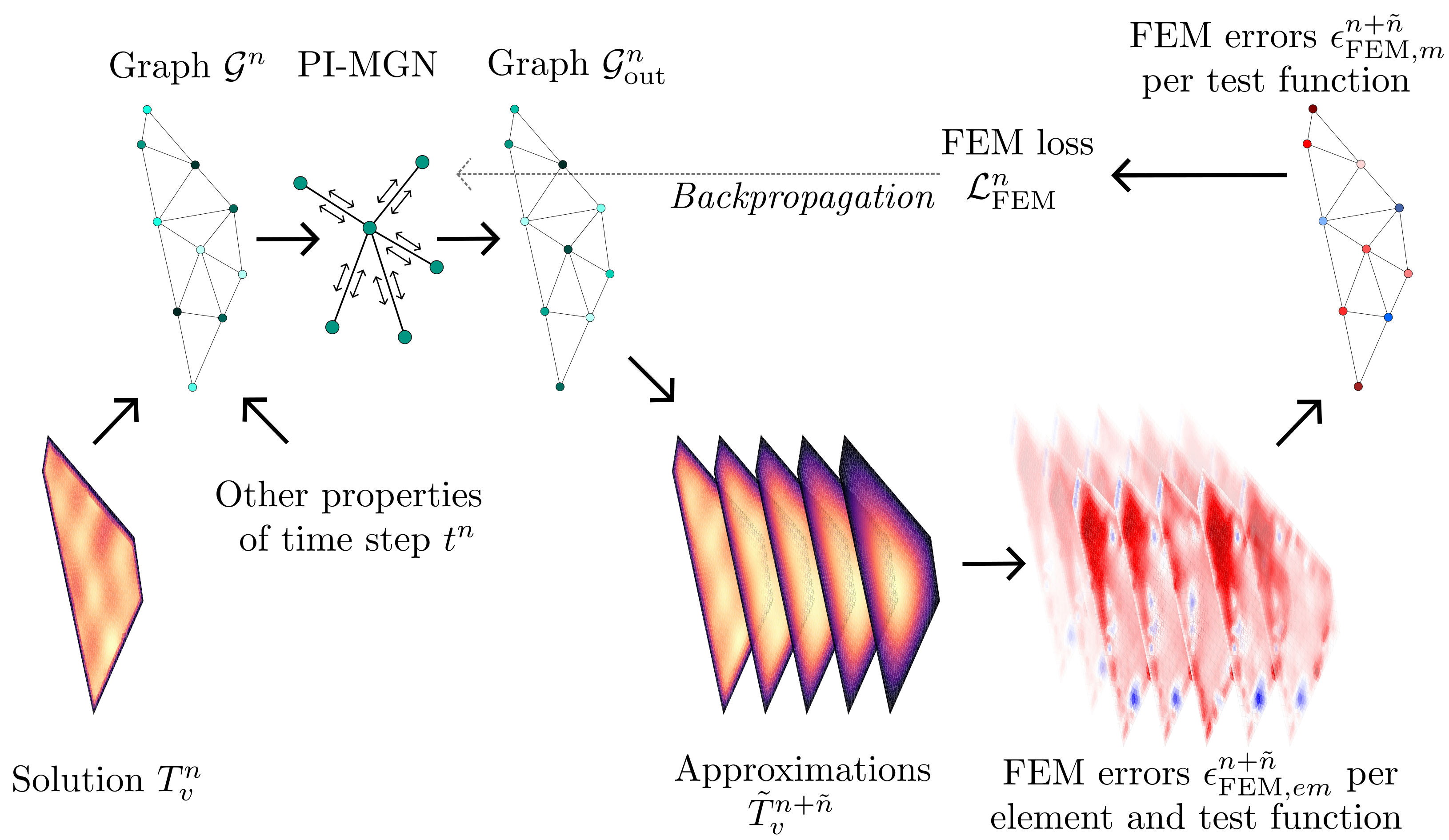
Figure 1: Given a solution $T_{v}^{n}$ and additional properties of the time step $t^{n}$, a graph $G^{n}$ is assembled and passed to the PI-MGNs, which output a graph $G^{n}_{\text{out}}$. This graph contains the approximations $\tilde{T}_{v}^{n+\tilde{n}}$ of the next time steps $t^{n+\tilde{n}}$, where $\tilde{n}=1,...,N_{\text{TB}}$. Using the FEM, an element- and test function-wise error is calculated and summed up to a test function-wise error. Finally, the loss is calculated as the MSE of all errors to update the PI-MGN using backpropagation.

One optimization loop starts with the initial condition at $t^{0}$ of a problem and assembles a graph $\mathcal{G}^{0}$ to update the PI-MGN. After this step, the time step $t^{N_{\text{TB}}}$ can be initialized to perform another optimization step. This procedure is repeated until the last time step $t^{N_{\text{T}}}$ is reached. Then, the optimization loop processes the next problem. The epoch is finished when the optimization loop has been repeated for all considered training problems $p$. The full training procedure consists of a given number of epochs.

It is important to note that the method is fully applicable to nonlinear equations without restrictions. The loss can also be calculated directly and in parallel for multiple time steps without the need for inner solving iterations. Additionally, since the FEM naturally integrates the Neumann boundary conditions into the PDEs and the Dirichlet boundary conditions are strictly enforced in this work, the initial-boundary-value problem has only to be solved for Eq. 9. This directly avoids competing training losses and the resulting training difficulties [30].

Noise injection in physics-informed training

As the output of an MGN at the time step $n$ is part of the next input graph $\mathcal{G}^{n+N_{\text{TB}}}$, next-step models struggle with error accumulation. Noise injection proves to be an effective strategy for MGN [10] to reduce this error accumulation. The basic idea is to add an artificial error to the input so that the MGN must detect and minimize the error. Here, noise injection is introduced for physics-informed training. Using Gaussian noise $\epsilon\sim\mathcal{N}(0,\mathbf{I}\sigma)$, a noisy solution difference $(T_{v}^{n}+\epsilon_{v})-(T_{u}^{n}+\epsilon_{u})$ respectively approximation $(\tilde{T}_{v}^{n}+\epsilon_{v})-(\tilde{T}_{u}^{n}+\epsilon_{u})$ is used as a substitute to the exact solution difference during training. However, the noiseless solution $T_{v}^{n-1}$ respectively approximation $\tilde{T}_{v}^{n-1}$ is still inserted into Equation 9, enabling the PI-MGN to learn to output the correct solution of Equation 9 for a noisy input. As in [10], the noise is only added during training and not at inference.

3 Experiments

3.1 Training on small meshes

The PI-MGNs are evaluated on three different experiments (cf. Fig. 2), where the models face different numerical and learning challenges:

• Firstly, a 2D linear heat diffusion task on randomly varying L-shaped domains is considered. The model learns to handle unseen meshed geometries and different process conditions in the form of random initial conditions.

• The second experiment contains a PDE with a nonlinear, time- and material-dependent heat source and considers random 2D convex polygons with random material distribution. The model has to learn the influence of random arbitrary material fields on the solution of a nonlinear PDE.

• Finally, the method is applied to various 3D meshes with mixed boundary conditions, in particular hollow cylinders that are heated over time due to a Neumann boundary condition.

A describes the three experiments in more detail.

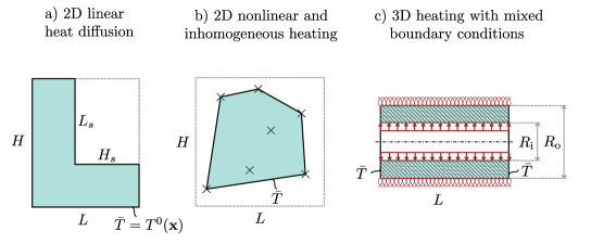
Figure 2: Schematic overview of the experiments. Figure a) shows an example of the L-shaped domain of a 2D linear heat diffusion experiment and Figure b) the initialization of an convex polygon with $7$ random points of the nonlinear experiment. Figure c) depicts a hollow cylinder of the 3D experiment with a heating boundary condition inside the cylinder (red arrows) and an adiabatic boundary condition at the outer surface (red coils).

Training

In the following, a problem $p$ contains a concrete specification of the experiments. In particular, it includes the specification of all material parameters, such as the diffusivity $\alpha$, the nonlinear source term $q(T)$ in Equation 1, a geometry $\Omega$, the initial condition $T^{0}$, the Dirichlet $\overline{T}\text{,}~{}\forall\mathbf{x}\in\Gamma$ and Neumann boundary conditions $h_{\mathcal{N}}\text{,}~{}\forall\mathbf{x}\in\partial\Omega_{\mathcal{N}}$. All experiments consider a total number of $100$ randomly generated problems. $75$ of these problems are selected randomly for training, while the other $25$ are used for validation. Training is repeated over $5$ random seeds, and each training consists of $500$ epochs with mini-batches comprised of $2$ graphs. The Adam [29] optimizer with an exponential learning rate decay from $110-3$ to $110-5$ is used. The gradient norm is clipped to $1$.

PI-MGN

All PI-MGNs consist of $12$ message passing steps and output the predicted solution of the next $20$ simulation steps. Each MLP consists of $2$ layers of $128$ neurons and uses a rectified linear unit (ReLU) activation function between layers and a layer norm [31] at the end. The input vector of node features, edge features and global features respectively is linearly encoded to a latent vector of the hidden dimension of $128$. The latent vector of size $128$ is decoded by a CNN to output a vector of length $20$, containing the solution approximation of $20$ time steps. The setup of the CNN follows previous work [13], consisting of $2$ layers with $1$ input channel, $8$ hidden channels and $1$ output channel, a kernel stride of $15$ respectively $10$ and a stride of $4$ respectively $1$.

Simulation and Evaluation

All problems are evaluated for a total amount of $100$ time steps, starting from $t^{0}=$0\text{\,}\mathrm{s}$$ and progress until $t^{N_{t}}=$1\text{\,}\mathrm{s}$$ is reached with a fixed time step $\Delta t=$0.01\text{\,}\mathrm{s}$$. For evaluation, FEM-solutions from the open-source package scikit-fem [32] serve as a ground truth reference. The FEM-solutions solve the same equations and time steps as the PI-MGNs for comparability. These FEM-solutions are in no way used for PI-MGN training. They only serve as ground truth to assess the quality of PI-MGN solutions after training. A normalized $L_{2}$ error

$$\epsilon_{L_{2},\text{norm}}=\frac{\left(\sum_{n=1}^{N_{t}}\sum_{v=1}^{N_{\varphi}}\left|\tilde{T}_{v}^{n}-T_{v}^{n}\right|^{2}\right)^{1/2}}{\left(\sum_{n=1}^{N_{t}}\sum_{v=1}^{N_{\varphi}}\left|T_{v}^{n}\right|^{2}\right)^{1/2}}$$ (10)

is used to measure the deviation of the PI-MGN prediction to the ground truth. For visualizing error distributions, a relative metric

$$\epsilon_{\text{rel}}^{n}=\frac{\tilde{T}_{v}^{n}-T_{v}^{n}}{\underset{v,n}{\max}(T_{v}^{n})-\underset{v,n}{\min}(T_{v}^{n})}$$ (11)

is applied.

Baselines

The PI-MGNs are compared to data-driven MeshGraphNets [10] and to PI-GGNs from [24], which train graph Chebyshev convolutional neural network (GCCN) with the FEM for solving forward and inverse stationary problems of a single geometry.

For the DD-MGNs baseline, the ground truth FEM data $T_{v}^{n}$ is integrated into the training process, which amounts to $75$ simulations per experiment and per repetition for training and $25$ for validation. Therefore, the loss function in Equation 9 is replaced by a data-based MSE loss

$$\mathcal{L}_{\text{data}}^{n}=\frac{1}{N_{\text{TB}}N_{\varphi,\mathcal{F}}}\sum_{\tilde{n}=1}^{N_{\text{TB}}}\sum_{v=1}^{N_{\varphi,\mathcal{F}}}\left|\tilde{T}_{v}^{n+\tilde{n}}-T_{v}^{n+\tilde{n}}\right|^{2}\text{.}$$ (12)

Analogous to the physics-informed loss $\mathcal{L}_{\text{FEM}}^{n}$, the data loss measures the deviation of all $N_{\text{TB}}$ approximations of the MGN for an input graph $\mathcal{G}^{n}$ at the time step $n$. Since the ground truth is now available during training, the noisy ground truth difference $(T_{v}^{n}+\epsilon_{v})-(T_{u}^{n}+\epsilon_{u})$ is added as an edge feature instead of the noisy approximation difference $(\tilde{T}_{v}^{n}+\epsilon_{v})-(\tilde{T}_{u}^{n}+\epsilon_{u})$, as in [10]. Apart from these two changes, everything remains the same for comparability, which includes all integrated extensions such as time bundling and global features. Hence, the DD-MGN and PI-MGN approaches differ only in their training and work identically during evaluation.

For the physics-informed baseline PI-GGN, the model is integrated into the PI-MGNs framework. Therefore, the GCCN of [24] replaces the MPN of this work and the absolute positions and the solution are added as node features as in [24], because the GCCN cannot consider edge features. The input size of the model is set to the experiment-specific numbers of node features and the output size to the time-bundling size $N_{\text{TB}}=20$. All other components of the GCCN remain the same as in [24], while all setups, such as the training setup, are consistent with the PI-MGN setup.

3.2 Generalization to large unseen meshes

In addition, the present work examines the ability of the PI-MGNs to generalize to large unseen meshes. Therefore, the pre-trained PI-MGNs and baseline models are applied on four unseen large mesh problems. The first two problems investigate the performance of the trained PI-MGNs to predict the 2D linear heat diffusion for large corrugated sheets consisting of $10$ respectively $100$ components. Subsequently, the models of the 2D nonlinear heating are applied on a large grid structure. The last problem considers the PI-MGNs of the 3D heatup with mixed boundary conditions applied on a long 3D hollow cylinder. A.4 contains a detailed description of the large mesh problems.

Ablation studies

Ablation studies investigate the effectiveness of the individual components of the PI-MGN architecture. In particular, the time bundling CNN decoder is compared to an MLP decoder and the sensitivity of the accuracy with respect to the time bundling size $N_{\text{TB}}$ is investigated. Further, the relative positional encoding is compared to an absolute positional encoding and the effectiveness of the global features and the training noise is investigated. Finally, the best-performing variants from the ablation study will be applied to the large mesh experiments to evaluate their generalization ability to generalize to large parts.

Speed comparison to the FEM

Finally, to evaluate the speed of the PI-MGN, the computation time is compared for the 2D nonlinear and inhomogeneous heating, as those are the most challenging for the FEM due to the nonlinearity.

4 Results

4.1 Training on small meshes

Qualitative comparison to the FEM

For a qualitative comparison of the accuracy and capability of the trained models, the solutions provided by PI-MGN are compared visually to the ground truth FEM on unseen part designs, material distributions, and process settings in Figures 3, 4 and 5. The results indicate that PI-MGN can produce accurate predictions that are visually similar to FEM solutions.

More precisely, Figure 3 a) shows a challenging example of the 2D linear heat diffusion experiment of Section 3.1, which contains a random initial condition with 4 hot spots on an unseen part design. It can be seen that the PI-MGN has learned to accurately predict the final solution at the last time step $t=$1\text{\,}\mathrm{s}$$. Figure 3 b) depicts the relative error $\epsilon_{\text{rel}}$.

Figure 4 shows a nonlinear heating problem from Section 3.1 with a challenging material distribution on a randomly selected seed to demonstrate that the PI-MGNs learn the influence of nonlinear material fields. Figure 4 a) shows the unseen material distribution $V_{\text{f}}$ on the unseen part. Figure 4 d) depicts the ground truth solution, showing that spots with low values of the material property result in a locally stronger heating. Figure 4 c) demonstrate that the PI-MGN precisely reproduces these solution. Figure 4 b) depicts the relative error between both simulations, showing that comparatively high deviations mostly appear close to the boundary.

Finally, the qualitative performance of the PI-MGN is compared to the FEM for an unseen and randomly selected instance of the 3D heating task with mixed boundary conditions of Section 3.1. Figure 5 a) shows the approximation of the PI-MGN, Figure 5 b) the ground truth and Figure 5 c) the relative error at the last time step $t=$1\text{\,}\mathrm{s}$$ of the simulation. A quarter of the unseen 3D hollow cylinders is cut off for visualization, providing a view of the solution inside the cylinder. As before, the PI-MGN and FEM solutions are in good agreement. Only a slight underestimation of the PI-MGN is visible.

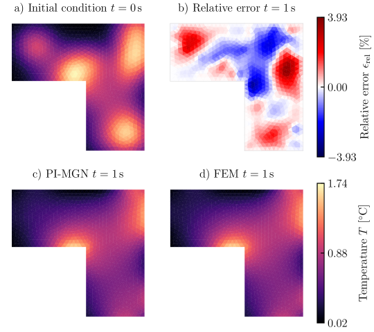
Figure 3: Comparison of the PI-MGN approximation to the FEM solution at the last time step $t=$1\text{\,}\mathrm{s}$$ for an unseen problem of the 2D linear experiment of Section 3.1. Figure 3 a) shows the randomly sampled initial condition on a new L-shaped mesh geometry. The relative error of the PI-MGN in Figure 3 b) measures the deviation of the PI-MGN approximation in Figure 3 c) from the ground truth in Figure 3 d).

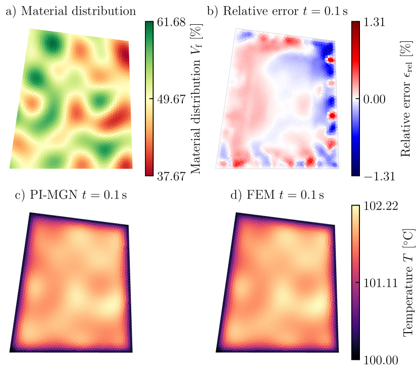
Figure 4: The PI-MGN solution is compared to the FEM for an nonlinear problem of the experiment of Section 3.1 after $t=$0.1\text{\,}\mathrm{s}$$. The geometry and material distribution (cf. Figure 4 a)) of the part was unseen during training. Figure 4 c) and Figure 4 d) show the approximation of the PI-MGN respectively the solution of the FEM. Figure 4 d) depicts the relative error between both solutions.

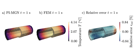
Figure 5: The 3D experiment of Section 3.1 with mixed boundary conditions. Figure 5 a) shows the solution of the PI-MGN at the last time step $t=$1\text{\,}\mathrm{s}$$ and Figure 5 b) the ground truth FEM solution. Figure 5 c) depicts the relative error of Figure 5 a) compared to Figure 5 b). A quarter of the 3D hollow cylinders is cut off for visualization in Figure 5 a), b) and c).

The results show that the PI-MGN can handle non-stationary and nonlinear PDEs in 2D and 3D, enabling visibly precise prediction for the unseen part designs, inhomogeneous material fields under new process conditions.

Comparison to baseline models

Figure 6 shows the performance of the PI-MGNs relative to the baselines DD-MGNs and PI-GGNs for all three experiments: The 2D linear heat diffusion (’2DL’), the 2D nonlinear heating (’2DNL’) and the 3D heating with mixed boundary conditions (’3DMB’). The mean $\mu_{L_{2},\text{norm}}$ and the standard deviation $\sigma_{L_{2},\text{norm}}$ of the normalized $L_{2}$ error $\epsilon_{L_{2},\text{norm}}$ over five training repetitions is displayed for each method, calculated for 25 unseen evaluation problems. The comparability of absolute values between experiments is limited as all values are normalized by their reference solution. For example, the mean temperature in the 2D nonlinear experiment is about $100\text{\,}\mathrm{\SIUnitSymbolCelsius}$, while it is $0\text{\,}\mathrm{\SIUnitSymbolCelsius}$ in the others.

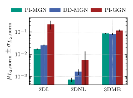
Figure 6: Comparison of the PI-MGNs to DD-MGNs and to the physics-informed baseline PI-GGN. Figure 6 shows the mean $\mu_{L_{2},\text{norm}}$ (bar) and the standard deviation $\sigma_{L_{2},\text{norm}}$ (black line onn bar) of the normalized $L_{2}$ error $\epsilon_{L_{2},\text{norm}}$, calculated for five training repetitions per model and experiment. Each bar group contains the results of the PI-MGNs, DD-MGNs and PI-GGNs for one of the three experiments of Section 3.1.

The PI-MGN outperforms the DD-MGN in two out of three experiments. The mean error $\mu_{L_{2},\text{norm}}$ of the data-driven training is almost $50\text{\,}\%$ higher for the 2D linear heatup experiment and approximately doubles for the 2D nonlinear and inhomogeneous heating. In contrast, the mean error of PI-MGNs is only slightly higher than that of DD-MGNs for the 3D heatup task. Here, the standard deviations overlap. Furthermore, the standard deviation $\sigma_{L_{2},\text{norm}}$ of the data-driven approach is larger in all three tasks, with an increase of up to $200\text{\,}\%$. For this 3D experiment, the physics does not vary as much across problems as in the other experiments, potentially explaining the similar performance across methods. However, training on similar problems may decrease generalization to out-of-distribution problems. This will be demonstrated in Section 4.2, where accuracy decreases for an adapted geometry.

The baseline PI-GGN model based on GCCN performs significantly worse for the 2D experiments, compared to the proposed PI-MGN and the DD-MGN baseline. For the 2D linear problem, the error is even more than an order of magnitude higher. In addition, the accuracy of the model is highly uncertain, which makes the training unreliable. The performance in the 3D mixed boundary task is slightly decreased, but still comparable. As for the DD-MGNs, it will be demonstrated in Section 4.2 that the trained models generalize worse to large meshes. This shows that the proposed MGN architecture plays an important role in the generalization capabilities and reliability of PI-MGNs, allowing the approach to perform well on non-stationary problems of unseen arbitrary meshes, material distributions and process conditions.

Overall, the proposed PI-MGN alleviates the expensive data creation process required for DD-MGNs while showing improved accuracy and consistency on different tasks. Further, the performance of the PI-MGN increases up to an order of magnitude, compared to the physics-informed baseline PI-GGN.

4.2 Generalization to large unseen meshes

Qualitative comparison to the FEM

The pre-trained models from Section 4.1 are applied to predict the time evolution on two large mesh experiments from Section 3.2 without any retraining or modification. The results are compared qualitatively to the FEM. Figure 7 a) shows the initial condition for a randomly selected model of the $5$ trained models. Even though the corrugated sheet mesh differs greatly from the L-shapes seen during training, the PI-MGN accurately predicts (cf. Figure 7 b)) the solution at the last time step when compared to the solution of the FEM in Figure 7 c). Figure 7 d) depicts the relative error between the PI-MGN and the FEM, showing that the PI-MGN tends to overestimates the solution. The highest error occurs at a point with high temperatures and temperature gradients, which are significantly larger than those observed during training.

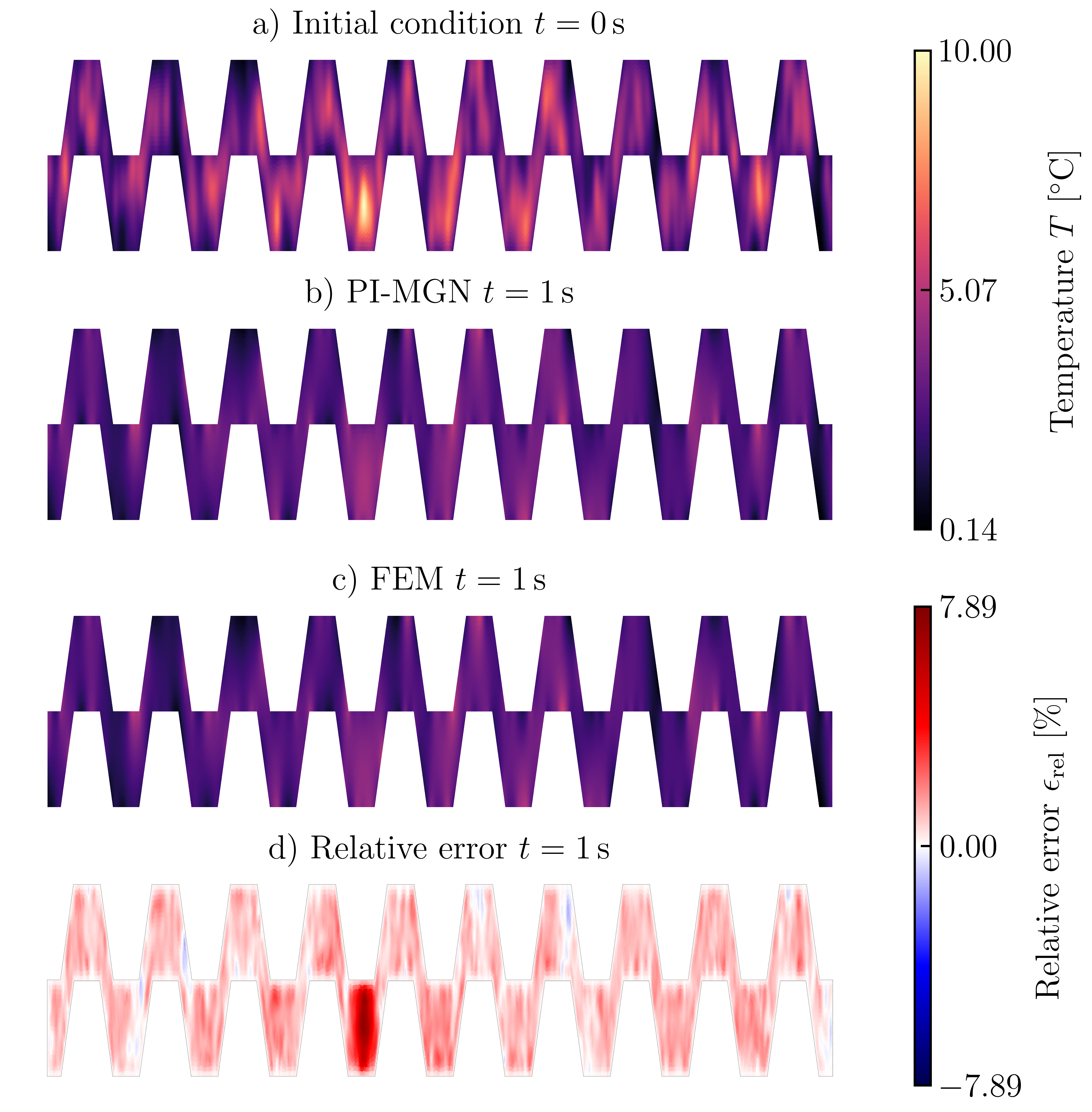
Figure 7: 2D linear heat diffusion experiment of Section 3.2 on a large mesh consisting of $10$ components. The part geometry and the random initial condition of Figure 7 a) was not part of the training. Figure 7 c) shows the solution of a PI-MGN, which was trained on the small meshes of Section 3.1. The deviation from the ground truth FEM solution (cf. Figure 7 c)) is depicted in Figure 7 d). For visualization purposes, the image is not to scale

The material distribution of the grid structure is depicted in Figure 8 a). The solution of the randomly chosen PI-MGN in Figure 8 c) is in good agreement with the FEM solution of Figure 8 d). As before, the local temperature increases depend on the surrounding material distribution and are especially prominent at the crossings of the grid structure. The PI-MGN provide accurate predictions and resolves fine local temperature changes. Interestingly, this is in contrast to classical PINNs, which have been reported to have a spectral bias toward learning low frequencies and may not be able to resolve such fine temperature changes [33, 34]. Figure 8 b) shows that the PI-MGN tends to overestimate the temperature at the bars and to underestimate it at the crossings.

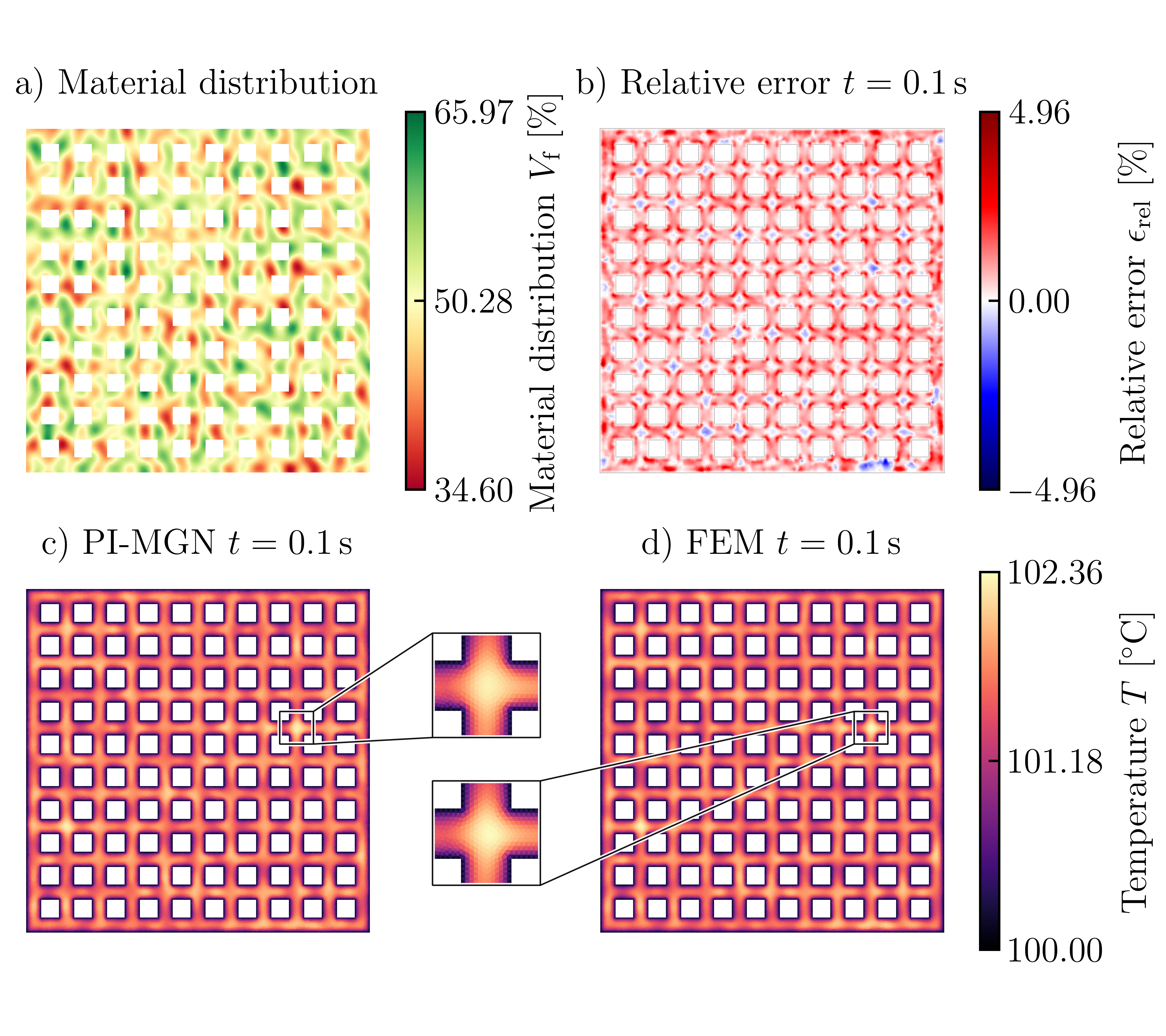
Figure 8: A trained PI-MGN predicts the solution of the nonlinear experiment of Section 3.2 on an large grid mesh. These PI-MGN is only trained on small polygon meshes. The large part contains an inhomogeneous material distribution, which is depicted in Figure 8 a). Figure 8 c) shows the approximation of the PI-MGN, Figure 8 d) the ground truth and b) the relative error the PI-MGN solution.

Comparison to baseline models

Figure 9 compares the PI-MGN, DD-MGN and PI-GGN accuracy on the four large mesh experiments: The 2D linear heat diffusion with a corrugated sheet part, which consists of $10$ repeating components (’2DL-10’) respectively $100$ repeating components (’2DL-100’), the 2D nonlinear and inhomogeneous heating of the grid structure (’2DNL-L’) and the 3D heating with mixed boundary conditions of the long hollow cylinder (’3DMB-L’). As before, the models from Section 4.1 are re-used without any further training or modification. Figure 9 shows the mean $\mu_{L_{2},\text{norm}}$ and standard deviation $\sigma_{L_{2},\text{norm}}$ of the normalized $L_{2}$ error across the $5$ repetitions.

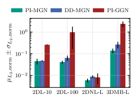
Figure 9: Performance of the PI-MGNs on the large mesh experiments of Section 3.2 compared to DD-MGNs and to PI-GGNs. The mean $\mu_{L_{2},\text{norm}}$ and the standard deviation $\sigma_{L_{2},\text{norm}}$ of the normalized $L_{2}$ error $\epsilon_{L_{2},\text{norm}}$ is calculated for five training repetitions per model and experiment. For each large mesh experiment, Figure 9 displays the mean $\mu_{L_{2},\text{norm}}$ (bar) and the standard deviation $\sigma_{L_{2},\text{norm}}$ (black line on bar) of the three models.

The DD-MGNs show comparable performance for the 2D linear heat diffusion task of the corrugated sheet mesh with 10 components. The mean error $\mu_{L_{2},\text{norm}}$ is slightly higher and the standard deviation $\sigma_{L_{2},\text{norm}}$ lower. For the other three problems, the PI-MGNs outperform the DD-MGNs. Hence, the physics-informed training of MGNs not only saves on expensive data creation but also improves generalization to larger meshes. A reason for that could be that the physics-informed training has to explore the solution during training, because no ground truth is known. The solution approaches the ground truth during training, but always fluctuates due to the model inaccuracy. Therefore, the model must predict a slightly different solution with respect to the imprecise output of the previous time step, which can help to stabilize the model rollout.

Ablation studies

The ablation studies conducted in B demonstrate the effectiveness of each component of the PI-MGN architecture in the small mesh experiments and its ability to generalize to larger, unseen meshes. For the training on small meshes, the PI-MGN shows the highest reliability in predicting accurate results across all experiments. Time bundling and global features are important components to achieve this reliability. Replacing the relative positional encoding with absolute positions as well as noise free training prove to be competitive alternatives. However, the results on the large meshes suggest that PI-MGN require relative encoding and robustness to noise to efficiently generalize beyond their training distribution.

Speed comparison to the FEM

Finally, Figure 10 compares the computation time of the PI-MGNs to the FEM for the 2D nonlinear and inhomogeneous heating. The results of the PI-MGNs are calculated on a GPU (NVIDIA^® GeForce^® RTX 2080) and on a CPU (Intel^® Xeon^® CPU E5-2680 v4 @ 2.40GHz), while the FEM results are only calculated on the CPU.

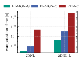
Figure 10: Speed comparison of the PI-MGNs to the FEM on the 2D nonlinear and inhomogeneous heating for the small meshes (’2DNL’) and large meshes (’2DNL-L’). Figure 10 compares the computation time of the PI-MGN on a GPU (’PI-MGN-G’) to its computation time on a CPU (’PI-MGN-C’) and to the FEM on a CPU (’FEM-C’). The GPU results are calculated on an NVIDIA^® GeForce^® RTX 2080 and the CPU results on an Intel^® Xeon^® CPU E5-2680 v4 @ 2.40GHz.

The PI-MGNs require on average only about $0.3\text{\,}\mathrm{s}$ on the GPU and $0.9\text{\,}\mathrm{s}$ on the CPU for the small meshes compared to approximately $50\text{\,}\mathrm{s}$ with the FEM on the same CPU. For the large mesh grid, the PI-MGNs output the solution in about $4\text{\,}\mathrm{s}$ on the GPU and in about $33.8\text{\,}\mathrm{s}$ on the CPU while the FEM solver requires $45\text{\,}\mathrm{m}\mathrm{i}\mathrm{n}$ on the CPU.

To sum up, the PI-MGNs trained on small meshes enable the most accurate and reliable predictions on large meshes over all considered learned models, while achieving speedups of several orders of magnitude compared to the FEM.

5 Conclusion and Outlook

This work introduces physics-informed MeshGraphNets (PI-MGNs) for fast, accurate and reliable finite element method (FEM) simulations of non-stationary problems on arbitrary mesh-geometries, material distributions and process conditions. PI-MGNs efficiently combine physics-informed neural networks (PINNs) and MeshGraphNets (MGNs) to overcome the time-intensive and cumbersome data creation process required for data-driven MeshGraphNets (DD-MGNs) while improving accuracy and generalization compared to existing PINNs. During training, the FEM equations are discretized and evaluated per mesh element, allowing to compute the physics-informed loss for multiple time steps and nonlinear problems directly and in parallel. The state of the art MGNs [10] are extended with additional methods such as time-bundling and global graph features, all of which empirically improve performance.

The PI-MGNs predict accurate solutions in good agreement with numerical FEM solvers for unseen arbitrary parts with inhomogeneous materials under changed process conditions. For a 2D heat diffusion problem, the PI-MGNs precisely predict the thermal cool down of unseen parts under random initialized temperature distributions. Further, the PI-MGNs learn to account for random material distributions in a part when predicting a nonlinear 2D heat release process. Finally, the approach accurately predicts the heating for 3D parts with mixed boundary conditions as a result of heat flow at the boundary.

The introduced physics-informed training of the MGNs is compared to a data-driven training approach and to a physics-informed neural FEM solver. Even though PI-MGNs require no simulation data during training, they perform on par with or better than the data-driven variant in terms of accuracy on all experiments. This advantage of the physics-based training is even more significant when generalizing to larger parts during evaluation. In contrast to the data-driven training, the PI-MGNs reliably predict accurate simulations on large unseen meshes when trained only on small and generic meshes. The existing physics-informed neural FEM solvers in literature use architectures and parameterizations that are shown to perform worse in all experiments for both small and large meshes, highlighting the importance of the proposed PI-MGNs. An ablation study reveals the individual importance of several components of the MGNs, such as time bundling and global features.

Overall, the PI-MGNs prove to be a reliable and accurate solver for the non-stationary and nonlinear FEM with strong generalization to unseen processes with new meshes consisting of inhomogeneous materials. In addition, the PI-MGNs are significantly faster and fully differentiable, making them a promising option for inverse design optimization. Here, the MGNs could also be extended to a Bayesian formulation to respect the model uncertainty during optimization. Finally, PI-MGNs could be applied to speed-up simulations with other challenging nonlinearities, such as contact or large deformation simulations.

6 Acknowledgement

This work has been performed in subprojects T2 and M2 of the DFG AI Research Unit 5339, funded by the Deutsche Forschungsgemeinschaft (DFG, German Research Foundation) – 459291153. This work is also part of the Heisenberg project ”Digitalization of fiber-reinforced polymer processes for resource-efficient manufacturing of lightweight components”, funded by the DFG (project no. 455807141). The authors thank the German Research Foundation for its financial support.

7 Declaration of Competing Interest

The authors declare that they have no known competing financial interests or personal relationships that could have appeared to influence the work reported in this paper.

Appendix A Experiments

A.1 Experiment 1: 2D linear heat diffusion

The first experiment (cf. Figure 2 a)) considers a heat diffusion problem on a 2D L-Shaped domain, setting the source term $q(T)=0$ in Equation 1 and the thermal diffusivity $\alpha$ to a constant value. The initial condition is described by a sum of $N_{\text{ic}}$ Gaussians

$$T^{0}(\mathbf{x})=\sum_{i=0}^{N_{\text{ic}}}a_{i}\exp\left(-\left(\frac{(x-x_{0,i})^{2}}{2\sigma_{x,i}}+\frac{(y-y_{0,i})^{2}}{2\sigma_{y,i}}\right)\right)\text{.}$$

The factors $a_{i}$ and the standard deviations $\sigma_{x,i},\sigma_{y,i}$ are randomly selected from uniform distributions. The means $x_{0,i},y_{0,i}\in\Omega\cup\partial\Omega$ are randomly selected node positions. The initial temperature on the boundary is fixed during the whole simulation, i.e., $\overline{T}=T^{0}(\mathbf{x})\text{,}~{}\forall\mathbf{x}\in\Gamma$. Therefore, the problem contains no Neumann boundary condition, i.e. $\partial\Omega_{\mathcal{N}}=\{\}$.

The 2D L-shaped domain is defined as the difference of two rectangles. The large one has length $L$ and height $H$ and the small rectangle the length $L_{\text{s}}=a_{\text{L}}L$ and the height $H_{\text{s}}=a_{\text{H}}H$, where $L$, $H$, $a_{\text{L}}$ and $a_{\text{H}}$ are selected randomly, cf. Figure 2 a). The small rectangle is randomly placed at one of the corners of the large domain and subtracted from the large rectangle to yield the final L-shaped domain. A total amount of $100$ L-shaped domains are created and remain the same for all five seeds. However, mesh selection and initial conditions are still randomized over seeds for training and validation. The exact definitions of the constants and the distributions of the randomly selected values are listed in Table 1.

Table 1: Constants and randomly defined values of Experiment 1, the 2D linear heat diffusion experiment.

Property	Symbol	Value	Unit
Initial-boundary value problem
Source term	$q$	0	$\mathrm{K}\mathrm{/}\mathrm{s}$
Thermal diffusivity	$\alpha$	$510-2$	$\mathrm{m}^{2}\mathrm{/}\mathrm{s}$
Number of Gaussians	$N_{\text{ic}}$	10	-
Summand weight	$a_{i}$	$\sim\mathcal{U}(0.5,1)$	$\mathrm{\SIUnitSymbolCelsius}$
Standard deviation $x$-direction	$\sigma_{x,i}$	$\sim\mathcal{U}(1/12,1/6)$	$\mathrm{m}^{2}$
Standard deviation $y$-direction	$\sigma_{y,i}$	$\sim\mathcal{U}(1/12,1/6)$	$\mathrm{m}^{2}$
Geometry - L-shape
Length	$L$	$\sim\mathcal{U}(0.5,1)$	$\mathrm{m}$
Height	$H$	$\sim\mathcal{U}(0.5,1)$	$\mathrm{m}$
Length factor	$a_{\text{L}}$	$\sim\mathcal{U}(1/3,2/3)$	-
Height factor	$a_{\text{H}}$	$\sim\mathcal{U}(1/3,2/3)$	-

A.2 Experiment 2: 2D nonlinear and inhomogeneous heating

This experiment (cf. Figure 2 b)) contains a nonlinear source term

$$q(T)=q(T,t,\mathbf{x})=\tilde{q}_{0}(\mathbf{x})\exp{\left(-CTt/t_{0}\right)}CT$$ (13)

in Equation 1, where $C=8/T_{0}$, $\tilde{q}_{0}(\mathbf{x})=q_{0}(1-V_{\text{f}}(\mathbf{x}))$ and $t_{0}$, $T_{0}$ and $q_{0}$ are constant. The factor $\tilde{q}_{0}$ depends on an inhomogeneous material property $V_{\text{f}}$

$$V_{\text{f}}(\mathbf{x})=V_{\text{f,0}}+\sum_{i=1}^{N_{f}}a_{i}\sin\left(k_{x,i}x+d_{x,i}\right)\sin\left(k_{y,i}y+d_{y,i}\right)\text{.}$$

These material distributions are remotely inspired by inhomogeneities which may occur in press forming processes of short fibre reinforced composites. The material field contains $N_{f}$ functions, each depending on a product of sine waves in $x$ and $y$-direction. The factor $a_{i}$, the wavenumbers $k_{x,i}$ and $k_{y,i}$ as well as function shifts $d_{x,i},d_{y,i}$ are randomly chosen from uniform distributions, while $V_{\text{f,0}}$ is a constant. Additionally, the diffusion coefficient

$$\alpha=\alpha(\textbf{x})=1/\left(V_{\text{f}}(\mathbf{x})/\alpha_{\text{f}}+(1-V_{\text{f}}(\mathbf{x}))/\alpha_{\text{m}}\right)$$ (14)

also depends on the inhomogeneous material distribution $V_{\text{f}}(\mathbf{x})$ as well as on the constants $\alpha_{\text{f}}$ and $\alpha_{\text{m}}$. The temperature at the initial condition $T^{0}$ and at the whole boundary $\overline{T}$ is set to $T^{0}=\overline{T}=T_{0}$. The considered domains are convex polygons. These are constructed by uniformly sampling $7$ points $x_{\text{P}}$ and $y_{\text{P}}$ in the 2D domain $\Omega=(0,L)\times(0,H)$, cf. Figure 2 b). Subsequently, the convex hull of the set of the seven points is chosen as the domain, yielding a convex polygon with $3$ to $7$ boundary points. Table 2 lists the values of the constants and distributions of the random quantities.

The polygons and material distributions $V_{\text{f}}(\mathbf{x})$ of the $100$ problems are randomly selected in a pre-processing step and fixed for all training seeds. The problem selection of the $75$ training and $25$ validation is randomized across the five seeds. As the heat source $q(T,t,\mathbf{x})$ depends on time and temperature, the temperature T is added as a node feature and the time is added as both, a global and a node feature. In addition, the material property, evaluated at the nodes, is added as a node feature.

To obtain a ground truth solution for this nonlinear equation from a numerical solver, the equation is linearized and solved in an inner loop for each time step for a total number of $100$ inner iteration or until the solution is converged, depending on what happens first.

Table 2: Constants and randomly defined values of Experiment 2, the 2D nonlinear and inhomogeneous experiment.

Property	Symbol	Value	Unit
Initial-boundary value problem
Reference time	$t_{0}$	$1$	$\mathrm{s}$
Reference temperature	$T_{0}$	$100$	$\mathrm{\SIUnitSymbolCelsius}$
Scaling factor	$q_{0}$	$20$	$\mathrm{K}\mathrm{/}\mathrm{s}$
Number of functions	$N_{f}$	$10$	-
Summand weight	$a_{i}$	$\sim\mathcal{U}(0,1/20)$	-
Wavenumber $x$-direction	$k_{x,i}$	$\sim\mathcal{U}(0,8\pi)$	$\mathrm{1}\mathrm{/}\mathrm{m}$
Wavenumber $y$-direction	$k_{y,i}$	$\sim\mathcal{U}(0,8\pi)$	$\mathrm{1}\mathrm{/}\mathrm{m}$
Wave shift $x$-direction	$d_{x,i}$	$\sim\mathcal{U}(0,2\pi)$	-
Wave shift $y$-direction	$d_{y,i}$	$\sim\mathcal{U}(0,2\pi)$	-
Median material property	$V_{\text{f,0}}$	$0.5$	-
Thermal diffusivity fibre	$\alpha_{\text{f}}$	$0.1$	$\mathrm{m}^{2}\mathrm{/}\mathrm{s}$
Thermal diffusivity matrix	$\alpha_{\text{m}}$	$0.01$	$\mathrm{m}^{2}\mathrm{/}\mathrm{s}$
Geometry - Convex polygon
Geometry length	$L$	$1$	$\mathrm{m}$
Geometry height	$H$	$1$	$\mathrm{m}$

A.3 Experiment 3: 3D heating with mixed boundary conditions

In the following, the PDE of A.1 is considered without a heat source $q(T)=0$ for a 3D hollow cylinder mesh with mixed boundary conditions (cf. Figure 2 c)).

The hollow cylinder has the length $L$, the outer radius $R_{\text{o}}$ and the inner radius $R_{\text{i}}=a_{\text{i}}R_{\text{o}}$, where $L$, $R_{\text{o}}$ and the fracture $a_{\text{i}}$ are randomly selected values. At the beginning, the temperature is $T^{0}=T_{0}$ across the domain. The temperature at the left and right cylinder boundary $\Gamma_{\text{l,r}}=\{\mathbf{x}=(x,y)\in\partial\Omega:x=0,L\}$ is also fixed to $\bar{T}=T_{0}$. A constant Neumann boundary condition is defined at the boundary surface at the inner side of the cylinder, i.e. at $\partial\Omega_{\text{i}}=\{\mathbf{x}=(x,y)\in\partial\Omega:y=R_{\text{i}}\}$ as $\alpha h_{\mathcal{N}}=h_{0}$. At the outer side of the cylinder $\partial\Omega_{\text{o}}=\{\mathbf{x}=(x,y)\in\partial\Omega:y=R_{\text{o}}\}$ an adiabatic Neumann boundary condition $\alpha h_{\mathcal{N}}=0$ is considered. The thermal diffusivity $\alpha$ is constant.

The initial learning rate is changed to $110-4$, but still decays to $110-5$. The $100$ meshes of the 3D hollow cylinders are the same for all five training seeds, but the part selection for the training and validation remains random for the individual seeds. The inner heat $h_{0}$ of the Neumann boundary condition is added as an additional node feature. The exact constants and the randomly selected value definitions are given in Table 3.

Table 3: Constants and randomly defined values of Experiment 3, the 3D heating experiment with mixed boundary conditions.

Property	Symbol	Value	Unit
Initial-boundary value problem
Source term	$q$	0	$\mathrm{K}\mathrm{/}\mathrm{s}$
Reference temperature	$T_{0}$	0	$\mathrm{\SIUnitSymbolCelsius}$
Thermal diffusivity	$\alpha$	$1$	$\mathrm{m}^{2}\mathrm{/}\mathrm{s}$
Inner heat constant	$h_{0}$	1	$\mathrm{m}~{}\mathrm{K}\mathrm{/}\mathrm{s}$
Geometry - Hollow cylinder
Length	$L$	$\sim\mathcal{U}(4,5)$	$\mathrm{m}$
Outer radius	$R_{\text{o}}$	$\sim\mathcal{U}(0.8,1)$	$\mathrm{m}$
Fracture radius	$a_{\text{i}}$	$\sim\mathcal{U}(0.6,0.8)$	$\mathrm{m}$

Table 4 provides an overview of the node, edge and global features used in the experiments as well as the output values of the PI-MGNs.

Table 4: Input and output features used in each experiment, including node, edge, and global input features, as well as the output features on the nodes.

Experiment	Node	Edge	Global	Outputs
2D Linear	$n_{\text{t}}$	$\mathbf{x}_{vu}$, $|\mathbf{x}_{vu}|$, $T_{vu}$	-	$T$
2D Nonlinear	$n_{\text{t}}$, $t$, $T$, $V_{\text{f}}$	$\mathbf{x}_{vu}$, $|\mathbf{x}_{vu}|$, $T_{vu}$	$t$	$T$
3D mixed BCs	$n_{\text{t}}$, $h_{0}$	$\mathbf{x}_{vu}$, $|\mathbf{x}_{vu}|$, $T_{vu}$	-	$T$

A.4 Large mesh problems of the experiments

For the first two problems, the models have to predict the 2D linear heat diffusion of A.1 for large corrugated sheets, which consist of repeating components of length $L$ and thickness $D$. The first problem considers a mesh consisting of $N_{\text{c1}}=10$ repeating components with $10\,840$ total mesh elements and the second of $N_{\text{c2}}=100$ components with $107\,592$ elements. The number of Gaussians for the initial condition is increased to $N_{\text{ic}}=1000$. As a result, the density of the Gaussians in the initial state in the two parts varies by a factor of $10$. These evaluation problems are multiple magnitudes larger larger than anything seen during training, as the training process for all methods uses meshes with $155$ to $524$ elements and $N_{\text{ic}}=10$ Gaussians.

The third problem considers the 2D nonlinear heating of A.2 for a grid structure. The grid part is a large rectangle with the length and height $L$ and contains $N_{\text{h}}=100$ rectangle holes equally distributed along the length and height direction and with a distance of $d_{\text{h}}$. The mesh of the grid contains $23\,296$ elements, while the training meshes contain between $148$ and $1122$ elements.

The last problem considers the 3D heatup with mixed boundary conditions of A.3 for a long 3D hollow cylinder, whose length $L$ is 40-50 times larger than that of the training meshes, while the outer radius $R_{\text{o}}$ and the inner radius multiplier $a_{\text{i}}$ correspond to the mean value of the training meshes. The other settings remain the same as in A.3.

The added constants and distributions of the randomly selected values for these experiments are listed in Table 5.

Table 5: Constants and randomly defined values of the large mesh experiments.

Property	Symbol	Value	Unit
Experiment 1: 2D Linear
Initial-boundary value problem
Number of Gaussians	$N_{\text{ic}}$	1000	-
Geometry - Corrugated sheet
Component length	$L$	$3$	$\mathrm{m}$
Component thickness	$D$	$0.5$	$\mathrm{m}$
Number of components part 1	$N_{\text{c1}}$	10	-
Number of components part 2	$N_{\text{c2}}$	100	-
Experiment 2: 2D Nonlinear
Geometry - Large rectangle
Length / Height	$L$	$4$	$\mathrm{m}$
Number of holes	$N_{\text{h}}$	$100$	-
Distance holes	$d_{\text{h}}$	$0.175$	$\mathrm{m}$
Experiment 3: 3D mixed BCs
Geometry - Long hollow cylinder
Length	$L$	$200$	$\mathrm{m}$
Outer radius	$R_{\text{o}}$	$0.9$	$\mathrm{m}$
Fracture radius	$a_{\text{i}}$	$0.7$	$\mathrm{m}$

Appendix B Ablation studies

The contribution and effectiveness of individual components of the proposed PI-MGN architecture is investigated in an ablation study. In each ablation, a component of the architecture is removed and, if necessary, replaced by a suitable alternative.

Training on small meshes

The first ablation uses absolute positions as node features instead of a relative positional encoding at the edges of the input graph of the PI-MGN (’abs. pos.’). Next, the training noise is left out, instead using unmodified predictions as input for the next MGN step (’w/o noise’). Then, global features are removed in Equation 5 of the PI-MGN (’w/o global’) and the CNN decoder of the model is replaced by an MLP decoder (’MLP decoder’). The last two ablations use different time bundling sizes $N_{\text{TB}}$, in particular $N_{\text{TB}}=10$ and $N_{\text{TB}}=50$ ( ’TBS-10’ respectively ’TBS-50’) instead of $N_{\text{TB}}=20$. These ablations investigate how accuracy changes when the number of model calls is doubled or approximately halved in the experiments.

Table 6 shows the results for PI-MGNs and all ablations. The table contains the mean $\mu_{L_{2},\text{norm}}$ and standard deviation $\sigma_{L_{2},\text{norm}}$ of the error $\epsilon_{L_{2},\text{norm}}$ over five training repetitions for 25 unseen problems per experiment.

Table 6: Ablation study of the PI-MGNs for five training repetitions per method and experiment, considering 25 unseen evaluation problems. The table displays $\mu_{L_{2},\text{norm}}\pm\sigma_{L_{2},\text{norm}}$, where $\mu_{L_{2},\text{norm}}$ is the mean and $\sigma_{L_{2},\text{norm}}$ the standard deviation of the normalized $L_{2}$ error $\epsilon_{L_{2},\text{norm}}$, each multiplied by $110+3$. The top-performing methods are highlighted in bold: blue for the best, green for the second-best, and yellow for the third-best.

Methods	2D Linear	2D Nonlinear	3D mixed BCs
PI-MGN	17.19 $\pm$ 1.13	0.73 $\pm$ 0.15	86.07 $\pm$ 2.97
abs. pos.	17.73 $\pm$ 0.96	0.97 $\pm$ 0.13	47.57 $\pm$ 18.37
w/o noise	16.08 $\pm$ 15.53	0.86 $\pm$ 0.16	88.53 $\pm$ 6.57
w/o global feature	16.37 $\pm$ 0.72	0.68 $\pm$ 0.05	162.71 $\pm$ 8.65
MLP decoder	173.52 $\pm$ 143.60	0.86 $\pm$ 0.15	85.13 $\pm$ 4.38
TBS-10	75.89 $\pm$ 125.50	0.77 $\pm$ 0.08	90.94 $\pm$ 9.73
TBS-50	21.80 $\pm$ 3.93	1.74 $\pm$ 0.06	88.37 $\pm$ 7.10

Only the proposed PI-MGNs architecture perform well in all experiments and consistently score within the top three models in terms of mean error $\mu_{L_{2},\text{norm}}$. The absolute position encoding shows comparable performance in two of the three experiments and even outperforms the PI-MGNs in the 3D experiment of A.3. However, the relative positional encoding is a more solid representation for generalization to geometries, which will be shown in Section 4.2. Removing the training noise leads to increased standard deviations in two of the three experiments, while the mean error remains comparable. Without global features, the prediction error slightly decreases for the 2D experiments, but almost doubles in the 3D case. The same applies for the MLP decoder ablation MLP decoder and the two time bundling size ablations TBS-10 and TBS-50. All of them perform similar to the PI-MGN in two of the experiments, but significantly worse in the third. These components of the architecture might not be necessary in all cases, but prove to be crucial for the reliability of the model. It is important to note that accuracy tends to decrease with fewer model calls (TBS-50), even though less error accumulation should increase accuracy. This phenomenon may be attributed to poorer generalization.

Generalization to large unseen meshes

Since training without noise and absolute position encoding showed the most competitive performance, these two ablations are compared to the proposed PI-MGNs architecture for generalization to large unseen meshes. Table 7 contains the results of the proposed PI-MGN architecture, the PI-MGN with absolute positional encoding (’abs. pos.’) and the noise-free variant (’w/o noise’). Therefore, the pre-trained models from the small mesh ablations are applied on the four large mesh experiments. The values of Table 7 are the mean $\mu_{L_{2},\text{norm}}$ and standard deviation $\sigma_{L_{2},\text{norm}}$ of the normalized $L_{2}$ error across the $5$ repetitions.

Table 7: Comparison of the PI-MGNs to the best performing variants of the small mesh ablations for the experiments on large meshes. The mean $\mu_{L_{2},\text{norm}}$ and the standard deviation $\sigma_{L_{2},\text{norm}}$ of the normalized $L_{2}$ error $\epsilon_{L_{2},\text{norm}}$ is calculated for five training repetitions per model and experiment. The tables displays the values in the format $\mu_{L_{2},\text{norm}}\pm\sigma_{L_{2},\text{norm}}$ multiplied by $110+3$. The best methods are highlighted in bold.

Methods	2DL-10	2DL-100	2DNL-L	3DMB-L
PI-MGN	45.42 $\pm$ 12.97	41.06 $\pm$ 6.32	5.93 $\pm$ 1.12	138.13 $\pm$ 33.55
abs. pos.	183.83 $\pm$ 82.99	285.54 $\pm$ 78.13	6.33 $\pm$ 1.43	766.06 $\pm$ 116.25
w/o noise	48.53 $\pm$ 26.34	34.00 $\pm$ 1.82	6.85 $\pm$ 0.81	240.78 $\pm$ 141.71

The PI-MGNs have the lowest error in 3 out of 4 problems. Only the noise free training slightly outperforms the PI-MGNs for the 2D linear heat diffusion problem of the corrugated sheet with 100 components, but clearly struggles to solve the long 3D hollow cylinder problem. The absolute positional encoding only performs well on the nonlinear task with the large grid structure and fails to provide accurate predictions in the other three problems. Remarkably, the noise-free training and absolute positional encoding ablations show decreased performance for the seemingly small change of the 3D problem setup, which considers only a longer hollow cylinder.

References

- [1] M. G. Larson, F. Bengzon, The Finite Element Method: Theory, Implementation, and Applications, Vol. 10 of Texts in Computational Science and Engineering, Springer, Berlin, Heidelberg, 2013. doi:10.1007/978-3-642-33287-6.
- [2] F. Moukalled, L. Mangani, M. Darwish, The Finite Volume Method in Computational Fluid Dynamics: An Advanced Introduction with OpenFOAM® and Matlab, Vol. 113 of Fluid Mechanics and Its Applications, Springer International Publishing, Cham, 2016. doi:10.1007/978-3-319-16874-6.
- [3] M. N. Özişik, H. R. B. Orlande, M. J. Colaço, R. M. Cotta, Finite Difference Methods in Heat Transfer, CRC Press, 2017.
- [4] S. P. Venkateshan, P. Swaminathan, Computational Methods in Engineering, Springer International Publishing, Cham, 2023. doi:10.1007/978-3-031-08226-9.
- [5] C. Zimmerling, C. Poppe, O. Stein, L. Kärger, Optimisation of manufacturing process parameters for variable component geometries using reinforcement learning, Materials & Design 214 (2022) 110423. doi:10.1016/j.matdes.2022.110423.
- [6] Z. Long, Y. Lu, X. Ma, B. Dong, PDE-Net: Learning PDEs from Data, in: Proceedings of the 35th International Conference on Machine Learning, PMLR, 2018, pp. 3208–3216.
- [7] J. Pfrommer, C. Zimmerling, J. Liu, L. Kärger, F. Henning, J. Beyerer, Optimisation of manufacturing process parameters using deep neural networks as surrogate models, Procedia CIRP 72 (2018) 426–431. doi:10.1016/j.procir.2018.03.046.
- [8] X. Guo, W. Li, F. Iorio, Convolutional Neural Networks for Steady Flow Approximation, in: Proceedings of the 22nd ACM SIGKDD International Conference on Knowledge Discovery and Data Mining, ACM, San Francisco California USA, 2016, pp. 481–490. doi:10.1145/2939672.2939738.
- [9] S. Bhatnagar, Y. Afshar, S. Pan, K. Duraisamy, S. Kaushik, Prediction of aerodynamic flow fields using convolutional neural networks, Computational Mechanics 64 (2) (2019) 525–545. doi:10.1007/s00466-019-01740-0.
- [10] T. Pfaff, M. Fortunato, A. Sanchez-Gonzalez, P. Battaglia, Learning Mesh-Based Simulation with Graph Networks, in: International Conference on Learning Representations, 2020.
- [11] M. Horie, N. Mitsume, Physics-Embedded Neural Networks: Graph Neural PDE Solvers with Mixed Boundary Conditions, Advances in Neural Information Processing Systems 35 (2022) 23218–23229.
- [12] Z. Li, K. Meidani, A. B. Farimani, Transformer for Partial Differential Equations’ Operator Learning, Transactions on Machine Learning Research (Dec. 2022).
- [13] J. Brandstetter, D. E. Worrall, M. Welling, Message Passing Neural PDE Solvers, in: International Conference on Learning Representations, 2021.
- [14] A. Sanchez-Gonzalez, J. Godwin, T. Pfaff, R. Ying, J. Leskovec, P. Battaglia, Learning to Simulate Complex Physics with Graph Networks, in: Proceedings of the 37th International Conference on Machine Learning, PMLR, 2020, pp. 8459–8468.
- [15] J. Sirignano, K. Spiliopoulos, DGM: A deep learning algorithm for solving partial differential equations, Journal of Computational Physics 375 (2018) 1339–1364. doi:10.1016/j.jcp.2018.08.029.
- [16] M. Raissi, P. Perdikaris, G. Karniadakis, Physics-informed neural networks: A deep learning framework for solving forward and inverse problems involving nonlinear partial differential equations, Journal of Computational Physics 378 (2019) 686–707. doi:10.1016/j.jcp.2018.10.045.
- [17] L. Sun, H. Gao, S. Pan, J.-X. Wang, Surrogate modeling for fluid flows based on physics-constrained deep learning without simulation data, Computer Methods in Applied Mechanics and Engineering 361 (2020) 112732. doi:10.1016/j.cma.2019.112732.
- [18] S. Amini Niaki, E. Haghighat, T. Campbell, A. Poursartip, R. Vaziri, Physics-informed neural network for modelling the thermochemical curing process of composite-tool systems during manufacture, Computer Methods in Applied Mechanics and Engineering 384 (2021) 113959. doi:10.1016/j.cma.2021.113959.
- [19] T. Würth, C. Krauß, C. Zimmerling, L. Kärger, Physics-informed neural networks for data-free surrogate modelling and engineering optimization – An example from composite manufacturing, Materials & Design 231 (2023) 112034. doi:10.1016/j.matdes.2023.112034.
- [20] H. Gao, L. Sun, J.-X. Wang, PhyGeoNet: Physics-informed geometry-adaptive convolutional neural networks for solving parameterized steady-state PDEs on irregular domain, Journal of Computational Physics 428 (2021) 110079. doi:10.1016/j.jcp.2020.110079.
- [21] P. Ren, C. Rao, Y. Liu, J.-X. Wang, H. Sun, PhyCRNet: Physics-informed convolutional-recurrent network for solving spatiotemporal PDEs, Computer Methods in Applied Mechanics and Engineering 389 (2022) 114399. doi:10.1016/j.cma.2021.114399.
- [22] X. Zhao, Z. Gong, Y. Zhang, W. Yao, X. Chen, Physics-informed convolutional neural networks for temperature field prediction of heat source layout without labeled data, Engineering Applications of Artificial Intelligence 117 (2023) 105516. doi:10.1016/j.engappai.2022.105516.
- [23] A. Kashefi, T. Mukerji, Physics-informed PointNet: A deep learning solver for steady-state incompressible flows and thermal fields on multiple sets of irregular geometries, Journal of Computational Physics 468 (2022) 111510. doi:10.1016/j.jcp.2022.111510.
- [24] H. Gao, M. J. Zahr, J.-X. Wang, Physics-informed graph neural Galerkin networks: A unified framework for solving PDE-governed forward and inverse problems, Computer Methods in Applied Mechanics and Engineering 390 (2022) 114502. doi:10.1016/j.cma.2021.114502.
- [25] A. Li, Y. J. Zhang, Isogeometric analysis-based physics-informed graph neural network for studying traffic jam in neurons, Computer Methods in Applied Mechanics and Engineering 403 (2023) 115757. doi:10.1016/j.cma.2022.115757.
- [26] M. Defferrard, X. Bresson, P. Vandergheynst, Convolutional Neural Networks on Graphs with Fast Localized Spectral Filtering, in: Advances in Neural Information Processing Systems, Vol. 29, Curran Associates, Inc., 2016.
- [27] P. W. Battaglia, J. B. Hamrick, V. Bapst, A. Sanchez-Gonzalez, V. Zambaldi, M. Malinowski, A. Tacchetti, D. Raposo, A. Santoro, R. Faulkner, C. Gulcehre, F. Song, A. Ballard, J. Gilmer, G. Dahl, A. Vaswani, K. Allen, C. Nash, V. Langston, C. Dyer, N. Heess, D. Wierstra, P. Kohli, M. Botvinick, O. Vinyals, Y. Li, R. Pascanu, Relational inductive biases, deep learning, and graph networks (Oct. 2018). arXiv:1806.01261, doi:10.48550/arXiv.1806.01261.
- [28] N. Freymuth, P. Dahlinger, T. Würth, S. Reisch, L. Kärger, G. Neumann, Swarm Reinforcement Learning For Adaptive Mesh Refinement (Oct. 2023). arXiv:2304.00818, doi:10.48550/arXiv.2304.00818.
- [29] D. P. Kingma, J. Ba, Adam: A method for stochastic optimization, arXiv preprint arXiv:1412.6980 (2014).
- [30] R. Bischof, M. A. Kraus, Multi-Objective Loss Balancing for Physics-Informed Deep Learning, Preprint, SSRN (2023). doi:10.2139/ssrn.4596537.
- [31] J. L. Ba, J. R. Kiros, G. E. Hinton, Layer normalization, stat 1050 (2016) 21.
- [32] T. Gustafsson, G. McBain, Scikit-fem: A Python package for finite element assembly, Journal of Open Source Software 5 (52) (2020) 2369. doi:10.21105/joss.02369.
- [33] Y. Cao, Z. Fang, Y. Wu, D.-X. Zhou, Q. Gu, Towards Understanding the Spectral Bias of Deep Learning, in: Proceedings of the Thirtieth International Joint Conference on Artificial Intelligence, International Joint Conferences on Artificial Intelligence Organization, Montreal, Canada, 2021, pp. 2205–2211. doi:10.24963/ijcai.2021/304.
- [34] U. B. Waheed, Kronecker Neural Networks Overcome Spectral Bias for PINN-Based Wavefield Computation, IEEE Geoscience and Remote Sensing Letters 19 (2022) 1–5. doi:10.1109/LGRS.2022.3209901.