Three-dimensional active nematic turbulence: chirality, flow alignment and elastic anisotropy

Abstract

Various active materials exhibit strong spatio-temporal variability of their orientational order known as active turbulence, characterised by irregular and chaotic motion of topological defects, including colloidal suspensions, biofilaments, and bacterial colonies. Here, we present a numerical study of three-dimensional (3D) active nematic turbulence, examining the influence of main material constants: (i) the flow-alignment viscosity, (ii) the magnitude and anisotropy of elastic deformation modes (elastic constants), and (iii) the chirality. Specifically, this main parameter space covers contractile or extensile, flow-aligning or flow tumbling, chiral or achiral elastically anisotropic active nematic fluids. The results are presented using time- and space-averaged fields of defect density and mean square velocity. The results also discuss defect density and mean square velocity as possible effective order parameters in chiral active nematics, distinguishing two chiral nematic states—active nematic blue phase and chiral active turbulence. This research contributes to the understanding of active turbulence, providing a numerical main phase space parameter sweep to help guide future experimental design and use of active materials.

Active nematic fluids are diverse synthetic and biological materials Shankar et al. (2022a); Sanchez et al. (2012); Wensink et al. (2012); Hardoüin et al. (2020); Wittmann et al. (2023); Peng et al. (2016); Sokolov et al. (2007); Dombrowski et al. (2004), characterized by orientational order along the director vector $\boldsymbol{n}$ and propelled by anisotropic active stress Hatwalne et al. (2004); Voituriez et al. (2005). A notable and rather ubiquitous dynamic state exhibited by active nematics is active turbulence Alert et al. (2022), characterized by continuous spatio-temporal defect proliferation and annihilation. This phenomenon is governed by the intricate interplay between defects within the director field and the structures of the velocity field Head et al. (2023). In three dimensions, the structure of active turbulence comprises a dynamic rewiring network of defect lines and loops Duclos et al. (2020); Urzay et al. (2017); Ž. Krajnik et al. (2020); Singh et al. (2023), where the diverse range of possible defect shapes and their interplay with the velocity field pose significant challenges for its understanding, control and possible applicability.

Approaches for studying 3D active turbulence include theoretical models of individual defect loops Binysh et al. (2020); Long et al. (2021); Houston and Alexander (2022), spectral analysis Urzay et al. (2017); Ž. Krajnik et al. (2020), and defect tracking and extracting the statistics of linked loops Romeo et al. (2023), defect curvature and length Digregorio et al. (2023); Binysh et al. (2020). Another possible approach is to extract the mean-field observables such as average defect density and squared velocity. The scaling of such observables with the activity was determined for single elastic constant and constant viscosity parameters Kralj et al. (2023); Digregorio et al. (2023). However, a systematic study of 3D active nematic turbulence for different elasticity, viscosity, and chirality material parameters also at different values of activities has not been performed yet. As shown also for 2D active nematics Giomi (2015); Alert et al. (2020); Thampi et al. (2014), a systematic numerical study can lead to better experimental control of active mater with different material properties and serve as a benchmark for theoretical models of activity-dependent dynamic regimes, instabilities, and coupled structures in the flow and orientation field.

In this paper, we show three-dimensional active nematic turbulence at different values of the main material parameters – i.e. (i) the flow-alignment viscosity parameter, (ii) the elastic constants of splay, twist, and bend deformation modes, and (iii) the intrinsic chirality. From numerical simulations of active dynamics, defect density and mean square velocity are extracted. The simulations are performed for contractile and extensile active materials and show distinct scalings with alignment parameter and average elastic constant, while elastic anisotropy has little effect on the mean-field averaged observables of active turbulence. For chiral active nematic turbulence, we show that increasing inverse chiral pitch $q_{0}$ increases the defect density and decreases the mean square velocity. At high values of $q_{0}$, a transition between the active nematic blue phase and chirality-affected active turbulence is observed. Distinctly, in the active nematic blue phase we observe effective jamming of the defect lattice and a strong drop in the magnitude of the flow field.

RESULTS AND DISCUSSION

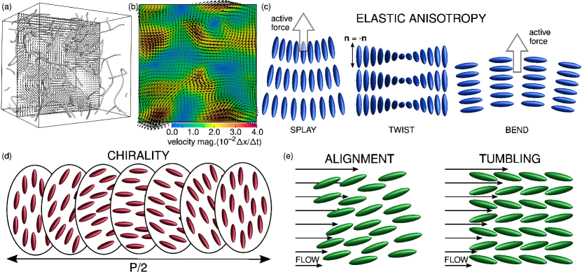
Figure 1: Active nematic turbulence in a three dimensional system. (a,b) A snapshot of an active turbulence showing (a) a disclination network (gray isosurfaces) with a director field cross-section (black rods) and (b) a cross section of the velocity field. (c–e) A schematic representation of mechanisms of (chiral) active turbulence: (c) different elastic modes of director deformations–splay, twist and bend–with the direction of the active force, (d) chiral structure of the director field with pitch length $P$, and (d) flow alignment and flow tumbling regime of the director field in shear flow.

We performed numerical simulations of 3D active nematic turbulence using the Beris-Edwards model of nematodynamics and the active stress tensor (Methods). We numerically solve the Q-tensor and the velocity field dynamics on a periodic grid using finite difference and lattice-Boltzmann numerical approaches, respectivelyCarenza et al. (2019); Zhang et al. (2016); Thampi et al. (2014); Kralj et al. (2023); Ž. Krajnik et al. (2020); Čopar et al. (2019). The main mechanisms of active turbulence that we focus on are visualised in Fig. 1.

Q-tensor field is shown in Fig. 1(a), where black rods show the director field as the main eigenvector of the Q-tensor and the gray isosurfaces show the degree of order representing the main eigenvalue. The degree of order is reduced near the core of disclination lines, which are string-like disordered structures spanning the simulation box. Figure 1(b) shows the velocity field and its magnitude for a selected snapshot of active turbulence. The nematic alignment has three main deformation modes, splay $\left(\nabla\cdot\boldsymbol{n}\right)^{2}$, twist $\left[\boldsymbol{n}\cdot\left(\nabla\times\boldsymbol{n}\right)-\frac{2\pi}{p_{0}}\right]^{2}$, and bend $\left[\boldsymbol{n}\times\left(\nabla\times\boldsymbol{n}\right)\right]^{2}$, each with its own elastic constant $K_{1}$, $K_{2}$, and $K_{3}$, respectively. Twist mode can be spontaneously favoured in chiral nematic fluids by incorporating a finite intrinsic chiral pitch length $p_{0}$ (Fig. 1(d)). Active force is computed as $-\alpha\nabla\cdot Q$ and is generated by the splay and bend deformations of the active constituents alignment Whitfield et al. (2017). The force direction in Fig. 1(c) is shown for extensile active materials ($\alpha>0$), opposite direction is expected for contractile materials ($\alpha<0$). Anisotropic viscosity of nematic fluids is in the Beris-Edwards model related to the flow-aligning parameter $\xi$, which is typically dependent on the shape of nematic building blocks and describes if they are aligning in flow gradient at a fixed angle, or constantly tumbling (Fig. 1(e)). Note that in principle, a general (passive or active) nematic fluid has 6 viscosity coefficients, 5 of which are independent de Gennes and Prost (1993). While the concepts of elastic anistropy, chirality, and flow alignment are well understood in equilibrium and driven nematic fluids, their effects on the irregular state of active turbulence is less understood, particularly in three dimensions. Here, we show how the properties of active turbulence depend on the material coupling constants determining the strength or anisotropy of elasticity, viscosity, and chirality.

Extensile, contractile, aligning, and tumbling nematics

The defect density and the average flow magnitude in active turbulence are affected by the viscosity parameters of the nematic fluid. Here, we vary the flow-aligning parameter $\xi$, effectively modelling the flow-tumbling and flow-aligning nematic fluids. At the highest value of the alignment parameter in the simulation ($\xi=1.5$), the cross-section of the director field and the velocity magnitude field show deformation at a larger scale compared to the lowest value of the aligning parameter at $\xi=0.2$ (Fig. 2 (a)). During the simulation, both the defect density (Fig. 2 (b)) and the mean square velocity (Fig. 2 (c)) fluctuate in time due to finite size effect of the simulation box. We consider the effect of the alignment parameter both for the extensile $(\alpha>0)$ and the contractile $(\alpha<0)$ active nematics. Independently from the sign of the active stress, the mean defect density is decreasing with an increase of the alignment parameter $\xi$ (Fig. 2 (d)). Differently, we observe that the mean velocity decreases with the alignment parameter for contractile active nematics and increases for extensile active nematics (Fig. 2 (e)). Different values of the flow-aligning parameter result in different Ericksen-Leslie coefficients of the anisotropic viscosity tensor (see Methods). Interestingly, no important change of active behaviour is observed directly at the transition between flow-aligning and flow-tumbling regime de Gennes and Prost (1993) at $\xi_{T}=\frac{9S_{\text{eq}}}{4+3S_{\text{eq}}}=0.86$ .

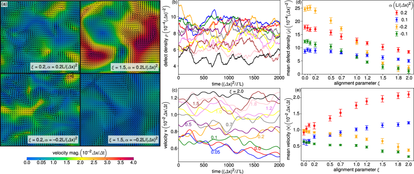
Figure 2: Dynamics of three-dimensional active nematic turbulence for extensile and contractile materials at different aligning parameters. (a) Cross-section of the velocity field magnitude (color map) and the director field (black rods) at two different activities $(\alpha=0.2\,L/(\Delta\mathrm{x})^{2}\text{ and }\alpha=-0.2\,L/(\Delta\mathrm{x})^{2})$ and two different alignment parameters $(\xi=0.2$ and $\xi=1.5)$. (b,c) Defect density and volume-averaged velocity over time in a dynamic steady state for activity $\alpha=0.1\,L/(\Delta\mathrm{x})^{2}$ and different alignment parameters. (d,e) The dependence of the mean defect density and the mean velocity on the alignment parameter $\xi$, computed from panels (b) and (c). The mean defect density decreases with the alignment parameter for extensile and contractile materials. The mean velocity shows an increasing trend with the alignment parameter for extensile materials ($\alpha>0$) and a decreasing trend for contractile materials ($\alpha>0$).

Role of elastic constants in active turbulence

Simulations at different values of the nematic elastic constants show two main results: (i) the defect density scales approximately linearly with the average elastic constant, and (ii) changing the elastic anisotropy—different elastic penalties of the splay, twist, and bend director deformation modes—has a minor effect on the active nematic defect density and average velocity magnitude.

Figure 3 shows the defect density and mean square velocity when varying the magnitude of the average elastic constant. We observe that in 3D active turbulence the mean inverse defect density increases with increasing average Frank elastic constant (Fig. 3(a)). Likewise, inverse velocity squared also increases approximately linearly with the average elastic constant. The observed behviour is in agreement with results from two-dimensional active turbulence where the defect density is inversely proportional to elastic constant magnitude Thampi et al. (2014); Giomi (2015).

Figure 4 shows the role of elastic anisotropy between the splay ($K_{1}$), twist ($K_{2}$) and bend ($K_{3}$) modes. We change the three elastic constants under the assumption of a fixed average elastic constant $\overline{K}=(K_{1}+K_{2}+K_{3})/3$ (see also Methods). Different values of the elastic constants provide relatively comparable results as seen on colormaps for the mean defect density in Fig. 4 (a) and mean velocity in Fig. 4 (b). The results in Fig. 4 (c) shows that the elastic anisotropy in the considered range has little effect on the dynamics of the active turbulence since both mean defect density and mean velocity stay roughly equal under the condition of same $\overline{K}$. With the condition of equal splay and twist modes ($K_{1}=K_{2}$, right panel in Fig. 4c), a slight increasing trend of the defect density is observed with increasing $K_{1}$ and $K_{2}$ and decreasing $K_{3}$.

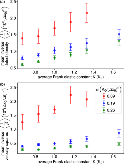
Figure 3: Defect density and mean square velocity as dependent on the average elastic constant. (a) Steady state mean inverse defect density and (b) steady state mean inverse velocity squared, both for three different activities. The average elastic constant was computed for different twist vs splay and bend elastic constants (see Methods).

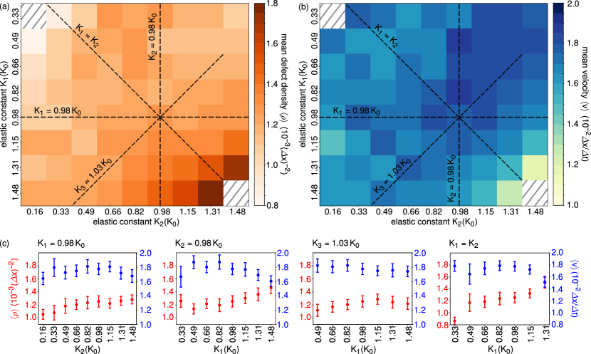
Figure 4: Effect of elastic anisotropy–different elastic constants–on the three-dimensional active turbulence for same average Frank elastic constant $\overline{\mathrm{K}}=\mathrm{K}_{0}$ and fixed activity $\alpha=0.2\,L/(\Delta\mathrm{x})^{2}$. (a) Mean defect density, (b) root mean square velocity and (c) selected cross-sections of the heat maps in (a,b), for different Frank elastic constants $K_{1}$ and $K_{2}$ (note that $K_{3}=3\overline{K}-K_{1}-K_{2}$). Small variability is observed, which is comparable to the fluctuations of the defect density and the mean velocity in time, as inherent to the chaotic active turbulent dynamics in finite volume.

Chiral active turbulence and transition to active blue phase

Material chirality in nematic systems can emerge as a result of chiral nematic building blocks, chiral dopants, or–in active systems–as a results of chiral dynamics of the active agents Fürthauer et al. (2012); Whitfield et al. (2017). In bulk 3D chiral active nematic, the intrinsic chirality increases the defect density and reduces the mean square velocity of active turbulence, notably already in the low chirality (i.e. large pitch) regime, as shown in Fig. 5. For example, for the chiral pitch equal to $p_{0}=200\,\Delta x$ (i.e. 89-times the active length $l_{a}=\sqrt{L/\alpha}$) at activity $\alpha=0.2\,L/(\Delta x)^{2}$, the defect density is increased by $48\%$ and the root mean square velocity decreased by $42\%$ compared to the dynamic steady state value for achiral active turbulence (Fig. 2(d,e)).

Upon further increasing chirality (i.e. reducing pitch) the passive chiral nematic is known to transition into 3D chiral orientational structures known as chiral blue phases I, II and III, and we observe a similar transition in active chiral nematics. Increasing chirality at fixed activity causes a steady increase of the defect density (Fig. 5(d)), up to a structure where defect lines of the active turbulence jam into a defect network, that one could identify as an effective active blue phase III (Fig. 5, first panel). Specifically, in active blue phase at pitch $p_{0}=25\,\Delta x$ and $\alpha=0.2\,L/(\Delta x)^{2}$, the defect density is 5-times larger than in achiral nematic turbulence case (Fig. 2(d)). An even stronger indication of an effective structural transition is the root mean square velocity that drops to $2\%$ compared to the achiral case at $\alpha=0.2\,L/(\Delta x)^{2}$. Such mean square velocity drop-off is uncharacteristic for active turbulence, but can be explained by no self-propulsion velocity of the double-twist cylinders and $-1/2$ disclinations that typically form the blue phase structure Metselaar et al. (2019). However, double twist cylinders (also called half-skyrmions) are predicted to be unstable at high enough activity and can split into two $+1/2$ disclinations Metselaar et al. (2019), which is in line with the transition between chiral active turbulence and active blue phase that we observe in Fig. 5.

We observe the distinct scaling of the disclination density and the mean square velocity near the transition between the active blue phase and the active turbulence. In Figure 5(b,c), we plot the inverse defect density and root mean square velocity dependence on the pitch length in proximity of the critical defect density $\rho_{c}$, critical mean velocity $v_{c}$ and critical chiral pitch $P_{c}$ of the blue phase-active turbulence transition. The slope of the graph shows that inverse defect density scales roughly as $(P_{0}-P_{c})^{0.6}$ and mean velocity as $(P_{0}-P_{c})^{0.3}$. Similar scaling is obtained for two different activities with a notable difference that at higher activity the blue phase-active turbulence transition occurs at smaller pitch lengths.

Figure 5: Chiral active turbulence and active blue phase. (a) Defect network at three different values of chiral pitch $\mathrm{P}_{0}$. (b) Mean inverse defect density dependence on the chiral pitch $\mathrm{P}_{0}$ for three different activities. The inset shows a zoomed-in area from $\mathrm{P}_{0}=25\,\Delta x$ to $\mathrm{P}_{0}=60\,\Delta x$. (c) Root mean square velocity dependence on the chiral pitch $P_{0}$. (d,e) Log-log plot of mean inverse defect density and root mean square velocity, respectively. The data in the log-log plots is plotted relative to the critical pitch length $P_{c}$ and the critical defect density. The values of $P_{c}=32\,\Delta x$ and $1/\rho_{c}=160\,\Delta x$ were chosen for the activity $\alpha=0.2\,L/(\Delta x)^{2}$, and the values of $P_{c}=34\,\Delta x$ and $1/\rho_{c}=170\,\Delta x$ for the activity $\alpha=0.15\,L/(\Delta x)^{2}$. The dashed line in (d) has a slope of $\mathrm{x}^{0.6}$ and the dashed line in (e) a slope of $\mathrm{x}^{0.3}$. (f) Zoom-in of the root mean square velocity graph in panel (c).

CONCLUSIONS

We explore dynamic reconfiguring network of disclination lines known as active turbulence using numerical simulations for selected main material parameters: chirality, flow alignement (anistropic viscosity), and elastic anistropy (different nematic elastic constants). The difference between extensile and contractile systems is observed in increasing or decreasing dependence of mean square velocity with the alignment parameter, showing the importance of the shape of active nematic building blocks Brand and Pleiner (1982). We confirm that defect density and mean square velocity are approximately inversely proportional to the magnitude of the average elastic constant, whereas the elastic anisotropy has only a small effect on the defect density and the mean square velocity of active turbulence. Though, we speculate that elastic anisotropy could affect the local structure of the defect lines ($+1/2$, $-1/2$ and twisted Binysh et al. (2020)) in the defect network. We performed simulations of an active chiral nematic and show the effective structural transition between chiral active turbulence and the active blue phase. The structures are distinct from each other and are separated by a continuous structural phase transition that we characterize by measuring the average inverse defect density and mean square velocity. Beyond the results reported here, the observed active blue phase dynamics would be (i) interesting to compare with blue phase dynamics due to thermal fluctuations Pišljar et al. (2022) and (ii) explored in the context of driving with external field, such as electric or magnetic fields Kikuchi et al. (2004) or activity gradients  Shankar et al. (2022b). An interesting aspect is also the difference between the transition to active turbulence in blue phases and in modulated cholesteric phase, for which a linear hydrodynamic instability was predicted for extensile materials Whitfield et al. (2017). While experimentally engineering 3D active blue phase materials can lead to very novel materials and phenomena, the effects of weak chirality that we show in the paper might be important also for present active nematic materials, since building blocks and processes in active matter are often chiral Fürthauer et al. (2012); Whitfield et al. (2017). Additionally, chiral symmetry breaking allows for additional active stresses Kole et al. (2021); Maitra et al. (2020); Hoffmann et al. (2020); Markovich et al. (2019).

More generally, this work is a contribution towards understanding the material-dependence of active nematic turbulence, to aid the experimental design and theoretical advances of active nematic phase Skogvoll et al. (2023); Pratley et al. (2023); Vélez-Cerón et al. (2023).

METHODS

Model equations of active nematodynamics

We simulate mesoscopic continuum description of active nematics using the adapted Beris-Edwards approach for active nematodynamics  Doostmohammadi et al. (2018); Čopar et al. (2019); Carenza et al. (2019). The nematic order is described by a traceless tensor order parameter $Q_{ij}$, with the director $\boldsymbol{n}$ as the main eigenvector, and evolves as

$$\left(\partial_{t}+v_{k}\partial_{k}\right)Q_{ij}-S_{ij}=\Gamma H_{ij},$$ (1)

where $\mathbf{v}$ is the fluid velocity and $\Gamma$ is the rotational viscosity coefficient. The generalized advection term $S_{ij}$ couples the nematic order and fluid velocity

$$S_{ij}= \left(\xi D_{ik}-\Omega_{ik}\right)\left(Q_{kj}+\frac{\delta_{kj}}{3}\right)$$

$$+\left(Q_{ik}+\frac{\delta_{ik}}{3}\right)\left(\xi D_{kj}+\Omega_{kj}\right)$$

$$-2\xi\left(Q_{ij}+\frac{\delta_{ij}}{3}\right)Q_{kl}W_{lk},$$

where $D_{ij}$ and $\Omega_{ij}$ are symmetric and antisymmetric part of the velocity gradient tensor $W_{ij}=\partial_{i}v_{j}$, and $\xi$ is the alignment parameter. The molecular field $H_{ij}$ drives system towards equilibrium of $Q_{ij}$

$$H_{ij}=-\frac{\delta F}{\delta Q_{ij}}+\frac{\delta_{ij}}{3}\mathrm{Tr}\frac{\delta F}{\delta Q_{ij}},$$

where $F$ is the Landau-de Gennes free energy

$$F =\int\left(\frac{A}{2}Q_{ij}Q_{ji}+\frac{B}{3}Q_{ij}Q_{jk}Q_{ki}+\frac{C}{4}\left(Q_{ij}Q_{ji}\right)^{2}\right.$$

$$+\frac{1}{2}L_{1}(\partial_{k}Q_{ij})(\partial_{k}Q_{ji})+\frac{1}{2}L_{2}(\partial_{i}Q_{jk})(\partial_{j}Q_{ik})$$

$$+\left.\frac{1}{2}L_{3}Q_{ij}(\partial_{i}Q_{kl})(\partial_{j}Q_{kl})\right)\mathrm{d}V.$$

Here, $A$, $B$ and $C$ are material parameters and $L_{1}$, $L_{2}$, and $L_{3}$ are elastic constants in the tensorial formulation of the elastic free energy. $L_{1}$, $L_{2}$, and $L_{3}$ can be computed from the elastic constants of the splay $K_{1}$, twist $K_{2}$, and bend $K_{3}$ deformation modes that are formulated within the director-based Frank free energy. Often, single elastic constant approximation $(L_{1}=L$, $L_{2}=L_{3}=0)$ is used, where splay, twist and bend elastic modes have equal contributions ($K_{1}=K_{2}=K_{3}=K$). In Figs. 3 and 4, we explore the role of elastic anistropy, i.e. how individual elastic modes influence the active nematic dynamics and we use non-zero $L_{1},L_{2}\text{ and }L_{3}$ elastic constants, following the relations

$$L_{1} =\frac{2}{27S^{2}}(-K_{1}+3K_{2}+K_{3}),$$

$$L_{2} =\frac{4}{9S^{2}}(K_{1}-K_{2}),$$ (2)

$$L_{3} =\frac{4}{27S^{3}}(-K_{1}+K_{3}).$$

In the formulation of the elastic constants in Eqs. 2, $K_{24}$ is equal to $\frac{K_{1}}{2}$ but is not relevant due to periodic boundary conditions. The flow field obeys the incompressibility condition and the Navier-Stokes equation,

$$\partial_{i}v_{i} =0,$$ (3)

$$\rho(\partial_{t}+v_{j}\partial_{j})v_{i} =\partial_{j}\Pi_{ij},$$ (4)

where $\rho$ is the fluid density and $\Pi_{ij}$ is the stress tensor, which consists a passive and an active term $\Pi_{ij}=\Pi_{ij}^{\text{passive}}+\Pi_{ij}^{\text{active}}$, where

$$\Pi_{ij}^{\text{passive}}= -p\delta_{ij}+2\eta D_{ij}+2\xi\left(Q_{ij}+\frac{\delta_{ij}}{3}\right)Q_{kl}H_{kl}$$ (5)

$$-\xi H_{ik}\left(Q_{kj}+\frac{\delta_{kj}}{3}\right)-\xi\left(Q_{ik}+\frac{\delta_{ik}}{3}\right)H_{kj}$$ (6)

$$+Q_{ik}H_{kj}-H_{ik}Q_{kj}-\partial_{i}Q_{kl}\frac{\delta F}{\delta\partial_{j}Q_{kl}},$$ (7)

$$\Pi_{ij}^{\text{active}} =-\alpha Q_{ij}.$$ (8)

Here, $p$ is the fluid pressure, $\eta$ is the isotropic viscosity, $\xi$ is the flow alignment parameter and $\alpha$ is the activity, which is positive in extensile materials and negative in contractile materials.

The coupled equations for the nematic order $Q_{ij}$ and fluid velocity $v_{i}$ are numerically solved using the hybrid lattice-Boltzmann approach Carenza et al. (2019); Zhang et al. (2016); Thampi et al. (2014); Kralj et al. (2023); Ž. Krajnik et al. (2020); Čopar et al. (2019), based on the finite difference method for solving the Q-tensor evolution (Eq. 1), and the D3Q19 lattice Boltzmann method for the incompressibility and the Navier-Stokes equation (Eqs. 3, 4).

Material parameters

In the paper, we consider a single elastic constant approximation for the material constants ($L_{1}\neq 0$, $L_{2}=0$, and $L_{3}=0$), except in Figs. 3 and 4. Changing the values of the elastic constants affects the nematic correlation length and in turn the resolution of the numerical mesh resolution. Accordingly, we compute the average Frank elastic constant

$$\overline{K}=\frac{1}{3}(K_{1}+K_{2}+K_{3})=\frac{9S^{2}}{2}\left(L_{1}+\frac{L_{2}}{3}\right)$$

from the mapping in Eqs. 2. To account for simulation results at different values of $\overline{K}$ in Fig. 3, we set $L_{1}=L$, vary the elastic constant $L_{2}$, and express the simulation results with a constant term $K_{0}=\frac{9S_{\text{eq}}^{2}}{2}L$. Here, $L$ represents the fixed value of the elastic constant as used in Figs. 2 and 5. In Figure 4, where we explore the role of the elastic anisotropy, we use the condition of a constant average Frank elastic constant $\overline{K}$ and choose the Frank elastic constants accordingly. From a given set of the Frank elastic constants, the tensorial elastic constants $L_{1}$, $L_{2}$, and $L_{3}$ are determined from a mapping given by Eqs. 2 evaluated at $S=S_{\text{eq}}$.

Using the alignment parameter $\xi$, rotational viscosity parameter $\Gamma$ and isotropic viscosity $\eta$ from the Beris-Edwards model of nematodynamics (Eqs. 1, 7), we can express the Ericksen-Leslie viscosity parameters de Gennes and Prost (1993); Denniston et al. (2001) that are typically formulated within the director-based approach to nematodynamics:

$$\alpha_{1} =\frac{\xi^{2}}{\Gamma}\frac{9S^{2}}{2}\left(3S^{2}-2S-1\right),$$

$$\alpha_{2} =-\frac{\xi}{\Gamma}\frac{S}{4}\left(3S+4\right)-\frac{1}{\Gamma}\frac{9S^{2}}{4},$$

$$\alpha_{3} =-\frac{\xi}{\Gamma}\frac{S}{4}\left(3S+4\right)+\frac{1}{\Gamma}\frac{9S^{2}}{4},$$

$$\alpha_{4} =\frac{\xi^{2}}{\Gamma}\left(S-\frac{2}{3}\right)^{2}+2\eta,$$

$$\alpha_{5} =-\frac{\xi^{2}}{\Gamma}\frac{S}{4}\left(3S-8\right)+\frac{\xi}{\Gamma}\frac{S}{4}\left(3S+4\right),$$

$$\alpha_{6} =-\frac{\xi^{2}}{\Gamma}\frac{S}{4}\left(3S-8\right)-\frac{\xi}{\Gamma}\frac{S}{4}\left(3S+4\right).$$

The flow-alignment parameter $\lambda$ in the director-based formulation then reads as $\lambda=\frac{\alpha_{2}+\alpha_{3}}{\alpha_{2}-\alpha_{3}}=\frac{3S+4}{9S}\xi$ and the flow-aligning to flow-tumbling transition occurs at $\lambda=1$ de Gennes and Prost (1993).

The overall results of the simulations are expressed in the units of the elastic constant $L$, rotational viscosity parameter $\Gamma$ and mesh resolution $\Delta x$. Mesh resolution is defined as $\Delta x=1.5\xi_{n}$, where $\xi_{n}$ is nematic correlation length defined as $\xi_{n}=\sqrt{L/(A+BS_{eq}+\frac{9}{2}CS_{eq}^{2})}$, where $S_{eq}=0.533$ is equilibrium degree of nematic order, $A=-0.43L/(\Delta x)^{2}$, $B=-5.3L/(\Delta x)^{2}$, $C=4.325L/(\Delta x)^{2}$ and $\eta=1.38/\Gamma$. The size of the simulation box is $201\times 201\times 201$ mesh points and periodic boundary conditions are used in all three spatial directions. $200\times 200\times 200$ simulation box is used in Fig. 2. The time step in simulations is set to $\Delta t=0.025(\Delta x)^{2}/(L\Gamma)$. To recover the simulation results in the SI units, one can use typical parameter values for active systems $L=3\,\text{pN}$, $\Delta x=2\,\upmu\text{m}$, and $\Gamma=10\,\text{(Pa s)}^{-1}$, roughly estimated from active turbulence in bacterial and microtubule systems Wolgemuth (2008); Sanchez et al. (2012) and viscoelastic properties of lyotropic nematics Zhang et al. (2018).

Data analysis

We define the defect density as the length of defect lines over a unit volume and compute it from the defect volume fraction of the regions where scalar order parameter is $S<0.4$ Kralj et al. (2023). In the next analysis step, we average either the defect density (Figs. 2 and 4) or the inverse defect density (Figs. 3 and 5) in time and calculate its standard deviation that is presented with error bars. For the velocity field, we compute the average of the velocity squared $\langle v^{2}\rangle_{V}$ over the complete simulation volume $V$ at given time. In Figs. 2, 4, and 5, we obtain the root mean square velocity as $\langle v\rangle=\sqrt{\langle v^{2}\rangle_{V}}$ and the variability (presented by error bars) from its standard deviation. In Fig. 3, the mean inverse velocity squared $\langle 1/v^{2}\rangle$ and its standard deviation are obtained from the time-dependence of the $1/\langle v^{2}\rangle_{V}$.

Author contributions

N.K. performed the numerical simulations and the analysis. M.R. and Ž.K. designed and supervised the research. All authors contributed to the writing of the manuscript.

Competing interests

The authors declare no competing interests.

References

- Shankar et al. (2022a) S. Shankar, A. Souslov, M. J. Bowick, M. C. Marchetti, and V. Vitelli, Nature Reviews Physics 4, 380 (2022a).
- Sanchez et al. (2012) T. Sanchez, D. T. N. Chen, S. J. DeCamp, M. Heymann, and Z. Dogic, Nature 491, 431 (2012), URL http://dx.doi.org/10.1038/nature11591.
- Wensink et al. (2012) H. H. Wensink, J. Dunkel, S. Heidenreich, K. Drescher, R. E. Goldstein, H. Lowen, and J. M. Yeomans, Proc. Natl. Acad. Sci. 109, 14308 (2012), URL http://dx.doi.org/10.1073/pnas.1202032109.
- Hardoüin et al. (2020) J. Hardoüin, J. Laurent, T. Lopez-Leon, J. Ignés-Mullol, and F. Sagués, Soft Matter 16, 9230 (2020), URL http://dx.doi.org/10.1039/d0sm00610f.
- Wittmann et al. (2023) R. Wittmann, G. P. Nguyen, H. Löwen, F. J. Schwarzendahl, and A. Sengupta, Communications Physics 6, 331 (2023).
- Peng et al. (2016) C. Peng, T. Turiv, Y. Guo, Q.-H. Wei, and O. D. Lavrentovich, Science 354, 882 (2016).
- Sokolov et al. (2007) A. Sokolov, I. S. Aranson, J. O. Kessler, and R. E. Goldstein, Physical review letters 98, 158102 (2007).
- Dombrowski et al. (2004) C. Dombrowski, L. Cisneros, S. Chatkaew, R. E. Goldstein, and J. O. Kessler, Physical review letters 93, 098103 (2004).
- Hatwalne et al. (2004) Y. Hatwalne, S. Ramaswamy, M. Rao, and R. Simha, Phys. Rev. Lett. 92, 118101 (2004), URL http://dx.doi.org/10.1103/PhysRevLett.92.118101.
- Voituriez et al. (2005) R. Voituriez, J. F. Joanny, and J. Prost, Europhys. Lett. 70, 404 (2005), URL http://dx.doi.org/10.1209/epl/i2004-10501-2.
- Alert et al. (2022) R. Alert, J. Casademunt, and J.-F. Joanny, Annu. Rev. Condens. Matter Phys. 13 (2022), URL http://dx.doi.org/10.1146/annurev-conmatphys-082321-035957.
- Head et al. (2023) L. C. Head, C. Dore, R. Keogh, L. Bonn, A. Doostmohammadi, K. Thijssen, T. Lopez-Leon, and T. N. Shendruk, arXiv preprint arXiv:2306.05328 (2023).
- Duclos et al. (2020) G. Duclos, R. Adkins, D. Banerjee, M. S. E. Peterson, M. Varghese, I. Kolvin, A. Baskaran, R. A. Pelcovits, T. R. Powers, A. Baskaran, et al., Science 367, 1120 (2020), URL http://dx.doi.org/10.1126/science.aaz4547.
- Urzay et al. (2017) J. Urzay, A. Doostmohammadi, and J. M. Yeomans, J. Fluid Mech. 822, 762 (2017), URL http://dx.doi.org/10.1017/jfm.2017.311.
- Ž. Krajnik et al. (2020) Ž. Krajnik, Ž. Kos, and M. Ravnik, Soft Matter 16, 9059 (2020), URL http://dx.doi.org/10.1039/c9sm02492a.
- Singh et al. (2023) A. Singh, P. H. Suhrcke, P. Incardona, and I. F. Sbalzarini, Physics of Fluids 35, 105155 (2023).
- Binysh et al. (2020) J. Binysh, Ž. Kos, S. Čopar, M. Ravnik, and G. P. Alexander, Phys. Rev. Lett. 124, 257 (2020), URL http://dx.doi.org/10.1103/PhysRevLett.124.088001.
- Long et al. (2021) C. Long, X. Tang, R. L. B. Selinger, and J. V. Selinger, Soft Matter 17, 2265 (2021), URL http://dx.doi.org/10.1039/d0sm01899f.
- Houston and Alexander (2022) A. J. Houston and G. P. Alexander, Physical Review E 105, L062601 (2022).
- Romeo et al. (2023) N. Romeo, J. Slomka, J. Dunkel, and K. J. Burns, arXiv preprint arXiv:2306.01062 (2023).
- Digregorio et al. (2023) P. Digregorio, C. Rorai, I. Pagonabarraga, and F. Toschi, arXiv preprint arXiv:2307.10103 (2023).
- Kralj et al. (2023) N. Kralj, M. Ravnik, and Ž. Kos, Physical Review Letters 130, 128101 (2023).
- Giomi (2015) L. Giomi, Physical Review X 5, 031003 (2015).
- Alert et al. (2020) R. Alert, J.-F. Joanny, and J. Casademunt, Nature Phys. 16, 682 (2020), URL http://dx.doi.org/10.1038/s41567-020-0854-4.
- Thampi et al. (2014) S. P. Thampi, R. Golestanian, and J. M. Yeomans, Philosophical Transactions of the Royal Society A: Mathematical, Physical and Engineering Sciences 372, 20130366 (2014).
- Carenza et al. (2019) L. N. Carenza, G. Gonnella, D. Marenduzzo, and G. Negro, Proc. Natl. Acad. Sci. 116, 22065 (2019), URL http://dx.doi.org/10.1073/pnas.1910909116.
- Zhang et al. (2016) R. Zhang, Y. Zhou, M. Rahimi, and J. J. de Pablo, Nat. Commun. 7, 13483 (2016), URL http://dx.doi.org/10.1038/ncomms13483.
- Čopar et al. (2019) S. Čopar, J. Aplinc, Ž. Kos, S. Žumer, and M. Ravnik, Phys. Rev. X 9, 031051 (2019), URL http://dx.doi.org/10.1103/PhysRevX.9.031051.
- Whitfield et al. (2017) C. A. Whitfield, T. C. Adhyapak, A. Tiribocchi, G. P. Alexander, D. Marenduzzo, and S. Ramaswamy, The European Physical Journal E 40, 1 (2017).
- de Gennes and Prost (1993) P. G. de Gennes and J. Prost, Physics of Liquid Crystals [PDF] (Clarendon Press, Clarendon Press, 1993), ISBN 0-19-852024-7.
- Fürthauer et al. (2012) S. Fürthauer, M. Strempel, S. W. Grill, and F. Jülicher, The European physical journal E 35, 1 (2012).
- Metselaar et al. (2019) L. Metselaar, A. Doostmohammadi, and J. M. Yeomans, The Journal of chemical physics 150 (2019).
- Brand and Pleiner (1982) H. Brand and H. Pleiner, Journal de Physique 43, 853 (1982).
- Pišljar et al. (2022) J. Pišljar, S. Ghosh, S. Turlapati, N. Rao, M. Škarabot, A. Mertelj, A. Petelin, A. Nych, M. Marinčič, A. Pusovnik, et al., Physical Review X 12, 011003 (2022).
- Kikuchi et al. (2004) H. Kikuchi, Y. Hisakado, K. Uchida, T. Nagamura, and T. Kajiyama, in Liquid Crystals VIII (SPIE, 2004), vol. 5518, pp. 182–189.
- Shankar et al. (2022b) S. Shankar, L. V. Scharrer, M. J. Bowick, and M. C. Marchetti, arXiv preprint arXiv:2212.00666 (2022b).
- Kole et al. (2021) S. Kole, G. P. Alexander, S. Ramaswamy, and A. Maitra, Physical Review Letters 126, 248001 (2021).
- Maitra et al. (2020) A. Maitra, M. Lenz, and R. Voituriez, Physical Review Letters 125, 238005 (2020).
- Hoffmann et al. (2020) L. A. Hoffmann, K. Schakenraad, R. M. Merks, and L. Giomi, Soft matter 16, 764 (2020).
- Markovich et al. (2019) T. Markovich, E. Tjhung, and M. E. Cates, New Journal of Physics 21, 112001 (2019).
- Skogvoll et al. (2023) V. Skogvoll, J. Rønning, M. Salvalaglio, and L. Angheluta, arXiv preprint arXiv:2302.03035 (2023).
- Pratley et al. (2023) V. J. Pratley, E. Caf, M. Ravnik, and G. P. Alexander, arXiv preprint arXiv:2310.19487 (2023).
- Vélez-Cerón et al. (2023) I. Vélez-Cerón, P. Guillamat, F. Sagués, and J. Ignés-Mullol, arXiv preprint arXiv:2307.11587 (2023).
- Doostmohammadi et al. (2018) A. Doostmohammadi, J. Ignés-Mullol, J. M. Yeomans, and F. Sagués, Nat. Commun. 9, 045006 (2018), URL http://dx.doi.org/10.1038/s41467-018-05666-8.
- Denniston et al. (2001) C. Denniston, E. Orlandini, and J. Yeomans, Physical Review E 63, 056702 (2001).
- Wolgemuth (2008) C. W. Wolgemuth, Biophys. J. 95, 1564 (2008), URL http://dx.doi.org/10.1529/biophysj.107.118257.
- Zhang et al. (2018) R. Zhang, N. Kumar, J. L. Ross, M. L. Gardel, and J. J. De Pablo, Proceedings of the National Academy of Sciences 115, E124 (2018).
Acknowledgements.
The authors acknowledge funding from Slovenian Research and Innovation Agency (ARIS) under contracts P1-0099, J1-50006, J1-2462, N1-0195. This result is also part of a project that has received funding from the European Research Council (ERC) under the European Union’s Horizon 2020 Research and Innovation Program (Grant Agreement No. 884928-LOGOS).Author contributions