MULTI-STAGE ALGORITHM FOR GROUP TESTING WITH PRIOR STATISTICS

Abstract

In this paper, we propose an efficient multi-stage algorithm for non-adaptive Group Testing (GT) with general correlated prior statistics. The proposed solution can be applied to any correlated statistical prior represented in trellis, e.g., finite state machines and Markov processes. We introduce a variation of List Viterbi Algorithm (LVA) to enable accurate recovery using much fewer tests than objectives, which efficiently gains from the correlated prior statistics structure. Our numerical results demonstrate that the proposed Multi-Stage GT (MSGT) algorithm can obtain the optimal Maximum A Posteriori (MAP) performance with feasible complexity in practical regimes, such as with COVID-19 and sparse signal recovery applications, and reduce in the scenarios tested the number of pooled tests by at least $25\%$ compared to existing classical low complexity GT algorithms. Moreover, we analytically characterize the complexity of the proposed MSGT algorithm that guarantees its efficiency.

I Introduction

Group testing (GT) aims to detect a small number of “defective” items within a large population by mixing samples into as few pooled tests as possible. The idea of GT was first introduced during World War II when it was necessary to discover soldiers infected with Syphilis. Dorfman proved in [1] that the required number of tests could be reduced if multiple blood samples were grouped into pools. Since it was first suggested, the problem of GT has been researched and generalized to many areas and applications, among them cyber security applications [2, 3, 4], pattern matching algorithms [5], image compression [6] and communications [7, 8]. Recently, GT has been examined again in view of COVID-19 [9, 10, 11, 12].

All these applications imply a strong connection between GT and Compressed Sensing (CS) [13] as two methods for sparse signal recovery that share common applications [14, 15, 16, 17]. The main difference between the two is that CS aims to recover a real-valued signal [13], while GT recovers a binary signal [18] or discrete-values [19, 20, 21, 12]. Thus, one can consider GT, which we study herein, as a Boolean CS [22].

The traditional research in the field of GT and its performance (i.e., the tradeoff between the number of pooled tests and recovery algorithm complexity) focused on the probabilistic model in which the items are identically distributed and independent [23, 18]. Recent research explores cases where prior information about objects correlation is available [24, 25, 26]. The motivation for this approach arises from the fact that correlated prior statistics holds the potential to achieve higher recovery rates and reduce the number of required tests. Correlated prior information exists in various domains relevant to GT. In numerous signal processing applications there is a correlation between different frequencies, time signals, or among different sensors that can be utilized to achieve more precise estimations [27, 13, 28]. In disease detection, one can leverage information about the proximity between individuals to save a significant amount of pooled tests [24]. The authors of [10, 11] proposed algorithms to exploit contact tracing information. In [29], a new probabilistic graph-based model and a suitable algorithm were proposed. Lau et al. [30] introduced a static graph-based model with correlated priors and demonstrated how the new problem can be translated into an optimization problem. All these works present solutions to the correlated objects problem in GT, nevertheless, their solutions are designed for specific models and may not be extended easily to others.

In this work, we introduce a practical non-adaptive Multi-Stage GT (MSGT) algorithm for correlated items with prior statistics. The proposed multi-stage algorithm employs a new variation of List Viterbi Algorithm (LVA) [31, 32, 33]. This variation was designed for GT to enable accurate low complexity recovery using fewer tests. In particular, in the LVA we suggest herein for the proposed MSGT, the key differences are: (1) the population sequence in GT replaces the time sequence in classical Viterbi Algorithm (VA), and (2) we use the aggregated sequence likelihood of the tested items instead of the general cost function presented in the original LVA [33]. The proposed algorithm can be applied for any statistical prior represented in a trellis [34], e.g., finite state machines and Markov processes. Using LVA, MSGT leverages those statistics to estimate the defective set efficiently, even in a regime below the Maximum Likelihood (ML) upper bound. Furthermore, we show how the algorithm’s parameters can be tuned to achieve the maximum probability of success without exceeding the limitation of the available computational capacity. Thus, as demonstrated, MSGT can work efficiently in practical regimes in which ML and MAP decoders for GT become infeasible. We derive a lower bound that considers the exact priors of the problem and provide analytical results that characterize the MSGT computational efficiency complexity. Our numerical results demonstrate that, in the regimes of interests for COVID-19 [35, 36, 37, 38] and for sparse recovery signal in signal processing [14, 15, 16, 13], the low computational complexity MSGT algorithm proposed herein can reduce in the tested scenarios the number of pooled tests by at least $25\%$, compared to existing classical ML and low complexity GT algorithms.

II Problem Formulation

Given a set of individuals $\mathcal{N}$, the objective in GT is to discover a small subset $\mathcal{K}$ of unknown defective items using the minimum number of measurements $T$. Let $N=|\mathcal{N}|$, $K=|\mathcal{K}|$ denote the total number of items and the number of defective items, respectively, where $K=\Theta(N^{\theta})$ for some $\theta\in\left[0,1\right)$. The binary vector $\mathbf{U}\in\left\{0,1\right\}^{N}$ represents the population, such that $U_{i}=1$ indicates that the $i$-th item is defective. We assume that the set of the individuals is sparse, such that $\theta\leq 1/3$, and that each item can be in one of 2 states: defective and non-defective. For each item there is some prior probability to be defective, $\left\{\mathbf{\pi}_{i}\right\}_{i=1}^{N}\in\left[0,1\right]^{N}$, and the correlation between the state of the $i$-th item and the states of the previous $\tau$ items is represented by $\mathbf{\Phi}_{i}\in\left[0,1\right]^{2^{\tau}\times 2^{\tau}}$. Here, $\tau\geq 1$ represents the memory of the underlying process considered.

For the non-adaptive GT, the testing matrix $\mathbf{X}\in\left\{0,1\right\}^{T\times N}$ is defined such that each row corresponds to a single pooled test, and each column corresponds to a single item. That is, the $i$-th pooled test is represented as a binary row vector: $X_{i}=\left[X_{i}\left(1\right),...,X_{i}\left(N\right)\right],\,i\in\left\{1,...,T\right\}$ whose elements are defined: $X_{i}\left(j\right)=1$ if the item with an index $j\in\left\{1,,...,N\right\}$ is included in the $i$-th pooled test, and otherwise $X_{i}\left(j\right)=0$. Then, the outcome of the $i$-th pooled test is given by

$$Y_{i}=\bigvee_{j\in\mathcal{K}}X_{i}\left(j\right)=\bigvee_{j=1}^{N}X_{i}\left(j\right)U_{j}$$

where $\bigvee$ is the boolean OR function as depicted in Fig. 1(a).

Given $\mathbf{X}$ and the outcome vector $Y$, the recovery success criterion in GT can be measured using various metrics [18]. The main metrics we will use herein are exact recovery and partial recovery. In terms of exact recovery, the goal is to detect the precise subset of defective items $\mathcal{K}$. Given the estimated defective set $\hat{\mathcal{K}}=\hat{\mathcal{K}}(N,K,\mathbf{X},Y)$, we define the average error probability by

$$P_{e}^{exact}\triangleq\frac{1}{\binom{N}{K}}\sum_{\mathcal{K}}P\left(\hat{\mathcal{K}}\neq\mathcal{K}\right).$$

In partial recovery, we allow a false positive (i.e., $|\hat{\mathcal{K}}\setminus\mathcal{K}|$) and false negative (i.e., $|\mathcal{K}\setminus\hat{\mathcal{K}}|$) detection rate. Thus, the partial success rate is given by:

$$P_{s}^{partial}\triangleq\frac{1}{\binom{N}{K}}\sum_{\mathcal{K}}\frac{\left|\hat{\mathcal{K}}\cap\mathcal{K}\right|}{K}.$$

To conclude, for a sparse subset of infected items of size $K$, out of a total of $N$ items, the goal in non-adaptive GT with correlated prior data items, is to design a $T\times N$ testing matrix $\mathbf{X}$ and an efficient and practical recovery algorithm that can exploit correlated priors, such that by observing $Y$ we can identify the subset of infected items with high probability and with feasible computational complexity. Thus, given the knowledge of the available computational resources, the test designer could design the testing matrix and the recovery algorithm to maximize the success probability.

III Efficient Multi-Stage Algorithm for Correlated Priors

In this section, we provide the efficient multi-stage algorithm for general correlated prior as given in Algorithm 1 and illustrated in Fig. 1. Initially, it employs low-complexity algorithms to reduce the search space (i.e., the possibly defective items) independently of prior correlations. Then, it employs a novel adaptation of the List Viterbi Algorithm (LVA) [33], designed for GT to enable accurate low-complexity recovery using fewer tests by exploiting the correlated prior information. The proposed LVA algorithm for GT can be applied for any statistical prior represented in a trellis diagram [34]. We now turn to the detailed pool-testing algorithm and computational complexity analysis for the proposed Algorithm 1. The proofs on the bounds in Theorems 1-4 and Proposition 1 given in this section are deferred to the Appendix as they cannot fit the scope of this extended abstract. In Section IV, we illustrate these bounds by simulation results (see Fig. 2).

III-A Pool-Testing Algorithm

III-A1 Testing Matrix and Pooling

The proposed multi-stage recovery algorithm is intended to work with any non-adaptive testing matrix, e.g., as given in [39]. To focus on the key methods, the testing matrix is generated randomly under a fixed optimal approximation with Bernoulli distribution of $p=\ln 2/K$ [40], using classical GT methods. The pooling and the outcome of the pooled tests are given by the process elaborated in Section II, and depicted in Fig. 1(a).

Algorithm 1 Multi-Stage Recovery Algorithm

Input: $\mathbf{X},Y,\{\mathbf{\pi}_{i},\mathbf{\Phi}_{i}\}_{i=1}^{N},K,L,\tau,\gamma$
      Output: $\hat{\mathcal{K}}$

1:Stage 1: Reduction of space search

2:$\mathcal{P}^{(DND)}\leftarrow\mathbf{DND}(\mathbf{X},Y)$

3:$\mathcal{D}^{(DD)}\leftarrow\mathbf{DD}\left(\mathbf{X},Y,\mathcal{P}^{(DND)}\right)$

4:$\mathcal{P}^{(DD)}\leftarrow\mathcal{P}^{(DND)}\setminus\mathcal{D}^{(DD)}$

5:Stage 2: Recovery exploiting prior info

6:$\{\mathbf{\pi}_{i},\mathbf{\Phi}_{i}\}_{i=1}^{N}\leftarrow\mathbf{updatePriors}\left(\{\mathbf{\pi}_{i},\mathbf{\Phi}_{i}\}_{i=1}^{N},\mathcal{P}^{(DD)},\mathcal{D}^{(DD)}\right)$

7:$\mathbf{Z}\leftarrow\mathbf{LVA}\left(L,\tau,\{\mathbf{\pi}_{i},\mathbf{\Phi}_{i}\}_{i=1}^{N}\right)$

8:$\mathbf{C}\leftarrow\{\}$

9:for $l\leftarrow 1$ to $L$ do

10:    if $K\leq\sum_{i}\left(\mathbf{Z}_{l,i}\right)\leq\gamma K$ then

11:         $\mathbf{V}^{(l)}\leftarrow\{\}$

12:         for $i$ s.t. $\mathbf{Z}_{l,i}=1$ do

13:             $\mathbf{V}^{(l)}\leftarrow\mathbf{V}^{(l)}\cup\{i\}$

14:         end for

15:         $c\leftarrow\mathbf{getAllCombinations}\left(\mathbf{V}^{(l)},K-\left|\mathcal{D}^{(DD)}\right|\right)$

16:         $\mathbf{C}\leftarrow\mathbf{C}\cup\left\{c\right\}$

17:    end if

18:end for

19:$\hat{\mathcal{K}}\leftarrow\mathbf{MAP}\left(\mathbf{X},Y,\mathbf{C},\{\mathbf{\pi}_{i},\mathbf{\Phi}_{i}\}_{i=1}^{N},\mathcal{P}^{(DD)},\mathcal{D}^{(DD)}\right)$

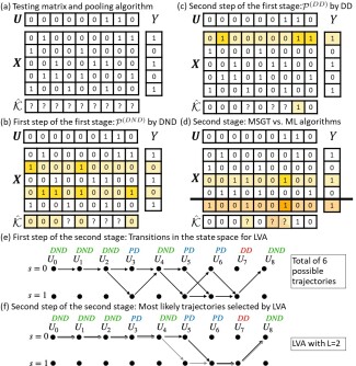
Figure 1: An example for MSGT algorithm vs. ML with $U\in\left\{0,1\right\}^{9}$ and $K=2$. (a) A random testing matrix is sampled and the test result $Y$ is calculated as given in Section III-A. In (b), the initial step of the first stage is depicted, wherein by DND algorithm, MSGT reveals $4$ DND items and $4$ possibly defective items $\mathcal{P}^{(DND)}$. Since items participating in negative tests must be non-defective, we mark all the participants in the two negative test results as non-defective. (c) demonstration of MSGT’s second step, the DD algorithm, where a single DD item is detected based on the first test result, as it is the only possibly defective item participating in this particular test. The two other positive test results do not contribute to our knowledge here because there is more than one possibly defective item participating in them. Thus, MSGT reveals $1$ DD item and $3$ possibly defective items $\mathcal{P}^{(DD)}$. Illustrated in (d) are the capabilities of ML decoder [22], for comparison with MSGT. If $T=4$, we refer only to the first 4 rows of $\mathbf{X}$ and ignore the last test result, having left with 3 possibly defective items that constitute two possibly defective sets of size $K=2$. Then, one of the two sets is chosen randomly by the ML decoder with a probability of $0.5$, leading to an error probability of $0.5$. In contrast, if $T=5$, based on the third and fifth test results, there is only one set of size $K=2$ for which the outcome $Y$ is obtained, and for this reason, $T=5$ will result in a successful decoding using ML decoder. As we further show, MSGT can successfully decode $\mathbf{U}$ in this scenario with only $T=4$. Figs. (e) and (f) shows the second stage of MSGT. (e) shows all the possible transitions in the state space that we consider in the LVA step, following the information obtained until (c). These transitions aggregate to a total of 6 trajectories (instead of 36 possible trajectories without the first stage). In (f), we assume $L=2$ in the LVA step, and the two most likely trajectories returned by LVA are displayed. It is important to note that given $K=2$, the black trajectory corresponds a valid population vector $\mathbf{U}$ with $2$ defective items, while the gray trajectory indicates an invalid population with $3$ defective items instead. Consequently, in the subsequent step, MSGT will extract 2 optional defective sets: $\left\{U_{6},U_{8}\right\}$ and $\left\{U_{7},U_{8}\right\}$, and will finally choose the most likely one using MAP estimator.

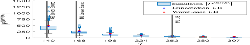
(a) Upper bound for possibly defective items after DND for $N=10000$, and $K=15$.

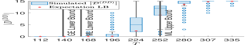
(b) Lower bound for definitely defective items after DD for $N=10000$, and $K=15$.

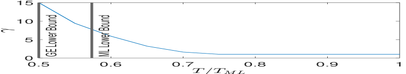
(c) Minimum $\gamma$ parameter to satisfies (2) for $N=500$, and $K=3$.

Figure 2: Numerical evaluation for theoretical results and bounds. The results in (a), (b), and (c) are over 1000 iterations. For ML Upper Bound (UB), $T_{ML}=(1+\epsilon)K\log_{2}N$, for any $\epsilon>0$ [22]. In particular, $\epsilon=0.25$ in the results presented herein.

III-A2 Recovery Process

The suggested recovery algorithm operates in two main stages. In the first stage, the algorithm efficiently identifies non-defective and definitely defective items without considering the prior correlated information. In the first step of this stage, we use the Definite Not Defectives (DND) algorithm [41, 42, 43, 23] (line 2). The DND algorithm marks items as ”definitely non-defective” if they are involved in a negative test, i.e., a test with a result of 0, as illustrated in Fig. 1(b). The output is the set of all the possibly defective items $\mathcal{P}^{(DND)}\subset\mathcal{N}$. Let $P_{e,a}^{(DND)}$ and $P_{e,u}^{(DND)}$ denote the error probability of DND in the average case and in its deviation (“worst-case”), respectively. The Theorems below give the upper bound on the expected number of possibly defective items and a “worst-case” upper bound after this step.

Theorem 1 ([12]).

Consider a group test with a Bernoulli testing matrix with $p=\ln{2}/K$, and $T$ tests as $N\rightarrow\infty$. Let $P_{e,a}^{(DND)}\triangleq N^{-\alpha\left(1-\ln{2}/K\right)/2}$ for $\alpha\triangleq T/K\log_{2}{N}$. The expected number of possibly defective items is bounded by

$$\mathbb{E}\left[\left|\mathcal{P}^{(DND)}\right|\right]\leq K+\left(N-K\right)P_{e,a}^{(DND)}.$$

Theorem 2.

Consider a group test with a Bernoulli testing matrix. For sufficiently large $T$ and any for $\gamma\geq 1$, the worst-case error probability of DND decoder is bounded by

$$P_{e,u}^{(DND)} \leq P_{e,a}^{(DND)}$$

$$+\left(1+\frac{\left(\gamma K-\left(K+\left(N-K\right)P_{e,a}^{(DND)}\right)\right)^{2}}{\left(N-K\right)P_{e,a}^{(DND)}\left(1-P_{e,a}^{(DND)}\right)}\right)^{-1}.$$

The parameter $\gamma$ controls LVA’s memory usage, thereby influencing its performance, as elaborated further on.

In the second step of the first stage, we use the Definite Defectives (DD) algorithm [23] (line 3), which goes over the test matrix and the test result, looking for positive pooled tests that include only one possibly defective item, as illustrated in Fig. 1(c). DD denotes those items as definitely defective items and outputs them as the set $\mathcal{D}^{(DD)}$. Since those items’ status becomes clear, we define a new set of possibly defective items, $\mathcal{P}^{(DD)}=\mathcal{P}^{(DND)}\setminus\mathcal{D}^{(DD)}$. The Theorem below gives the expected number of hidden defective items after this step.

Theorem 3.

Consider a group test with a Bernoulli testing matrix with $p=\ln{2}/K$, and $T$ tests as $N\rightarrow\infty$. The expected number of defective items that DD successfully detects is bounded by

$$\mathbb{E}\left[\left|\mathcal{D}^{\left(DD\right)}\right|\right]\geq K\left(1-N^{-\frac{\alpha}{2}\left(1-\ln{2}/K\right)^{N\cdot P_{e,a}^{(DND)}}}\right).$$ (1)

After these two steps, $\mathcal{P}^{(DD)}$ holds a new space search, and $\mathcal{D}^{(DD)}$ holds the already known defectives. This knowledge is acquired without utilizing any prior data, which we reserve for the second stage.

In the first step of the second stage, we translate the data we obtained in DND and DD, i.e., $\mathcal{P}^{(DD)}$ and $\mathcal{D}^{(DD)}$, to the state space in terms of transition probabilities, $\{\mathbf{\Phi}_{i}\}_{i=1}^{N}$, and initial probabilities, $\left\{\mathbf{\pi}_{i}\right\}_{i=1}^{N}$, so we can employ all the gathered information in the next steps (line 6). In the state space, the population sequence is parallel to time steps in the original LVA [33], and there are two possible states, $s\in\{0,1\}$, per $U_{i}$ item. The first indicates ”non-defective” (i.e., $s=0$) and the second indicates ”defective” (i.e., $s=1$). Fig. 1(e) demonstrates all the possible transitions in the state space.

In the second step, the suggested LVA for GT goes over the sequence of items, represented by a trellis (as depicted in Fig. 1(e)), and outputs the $L$ most likely trajectories in the state space (as depicted in Fig. 1(f)). Each trajectory is a sequence of $N$ states, representing a sequence of items, $\mathbf{U}\in\left\{0,1\right\}^{N}$, classified as either defective or non-defective. Following our design, LVA performs MAP decision (line 19) according to the given prior information. Thus, the output $\mathbf{Z}\in\{0,1\}^{L\times N}$ of this step, is a list of the $L$ most likely sequences of states (line 7), which constitute $L$ estimations for the $\mathbf{U}$. In practice, these sequences may include any number of defective items, necessitating further processing.

In the third step, we extract candidates for the defective set out of the $L$ estimated sequences in $\mathbf{Z}=[\mathbf{Z}_{1};\dots,\mathbf{Z}_{L}]$ (lines 9 to 18). Let $\mathbf{V}^{(l)}$ denote the set of items estimated as defective in sequence $\mathbf{Z}_{l},l\in\{1,\ldots,L\}$, i.e. $\mathbf{V}^{(l)}=\left\{i:\mathbf{Z}_{l,i}=1\right\}$. We ignore sequences $l$ in $\mathbf{Z}$ that contain less than $K$ defective items or more than $\gamma K$ defective items, for some $\gamma\geq 1$. That is, we consider only $\mathbf{Z}_{l}$ in which $K\leq\left|\mathbf{V}^{(l)}\right|<\gamma K$ as valid sequences, a regime considered without prior statistics in $\gamma K$-GT list decoding [44]. For each one of the valid sequences, we refer to all the $\begin{pmatrix}\left|\mathbf{V}^{(l)}\right|\\ K-\left|\mathcal{D}^{(DD)}\right|\end{pmatrix}$ combinations of size $K$ as candidates for $\hat{\mathcal{K}}$, and add them to the candidates list $\mathbf{C}$ (lines 15-16). The Proposition below provides a sufficient condition on $\gamma$, using the average error probability for optimal ML list decoder [44], s.t. MSGT achieves performance that we conjecture outperforms ML (as demonstrated in Section IV-2). This can be assumed as LVA used for this step of MSGT is an optimal MAP estimator (for sufficiently large $L$), known to outperform ML decoder [33].

Proposition 1.

Let $\eta\in\left(0,1\right)$ denote the average error probability of ML for any $T$. For $\gamma\geq 1$, MSGT can achieve an average error probability equal or less than $\eta$, if

$$T\geq\left(1-\eta\right)K\log_{2}\frac{N}{\gamma K}\left[1+f(\gamma)\right],$$ (2)

where $f(\gamma)=\frac{\eta\log_{2}{\frac{1-\eta}{\eta}}+\log_{2}{\frac{e}{1-\eta}}}{\eta\log_{2}{\frac{N-\gamma K}{K}}+\left(1-\eta\right)\log_{2}{\frac{\gamma K}{K}}}$.

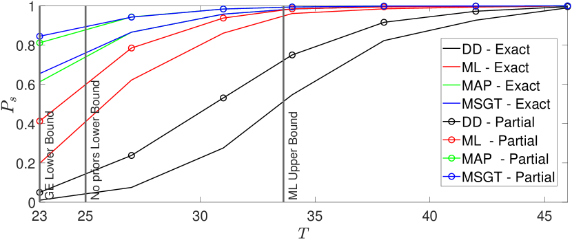
(a) $N=500$ and $K=3$.

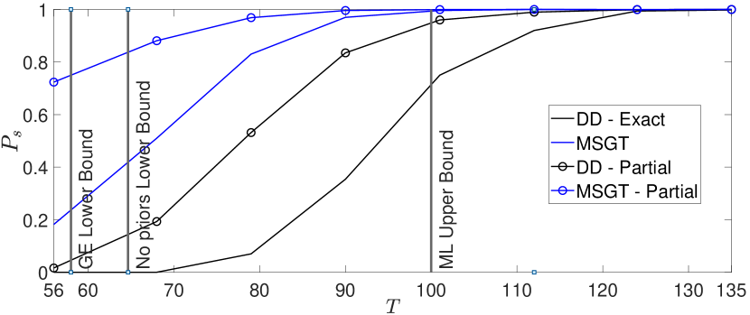
(b) $N=1024$ and $K=8$.

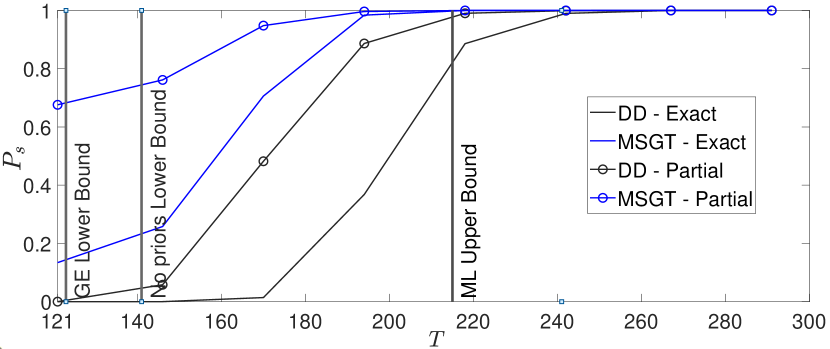
(c) $N=10000$ and $K=13$.

Figure 3: Success probability of MSGT, MAP, ML and DD over 1000 iterations. For ML Upper Bound, $T_{ML}=(1+\epsilon)K\log_{2}N$, for any $\epsilon>0$ [22]. In particular, $\epsilon=0.25$ in the results presented herein. A comparison to ML and MAP is not presented in (b) and (c), as they are not feasible for populations of those sizes due to the computational complexity burden.

At this point, we have in $\mathbf{C}$ a list of sets of size $K$, that are candidates to be our final estimation $\hat{\mathcal{K}}$, and we can calculate the probability of each one of them using $\{\mathbf{\pi}_{i},\mathbf{\Phi}_{i}\}_{i=1}^{N}$. Then, in the fourth step, the estimated defective set, $\hat{\mathcal{K}}$, is finally chosen using MAP estimator [45] out of the $\mathbf{C}$ (line 19).

If there are no valid sequences in $\mathbf{Z}$, we consider the paths with less than $K$ detections for partial recovery. We select the path in which the highest number of detections occur, and all the detections within it constitute our estimation, $\hat{\mathcal{K}}$.

Finally, one of the key features of the proposed MSGT algorithm is its low and feasible complexity in a practical regime compared to the ML and the MAP based GT. Both ML and MAP involve exhaustive searches, resulting in a complexity of $\mathcal{O}(\binom{N}{K}KN\log_{2}N)$ operations [22]. The Theorem below characterizes the computational complexity of MSGT.

Theorem 4.

Consider a group test for a population of size $N$ items out of which $K$ are defective and a Bernoulli testing matrix. The computational complexity of the MSGT algorithm is bounded by order of $\mathcal{O}\left(L\gamma^{K}KN\log_{2}N\right)$ operations.

Note that from Theorem 4 and Remark 1, it follows that the proposed MSGT algorithm performs $\mathcal{O}\left(\frac{1}{L}\left(\frac{N}{\gamma K}\right)^{K}\right)$ times fewer computational operations compared to MAP decoder.

III-A3 Discussion

To the best of our knowledge, MSGT is the first GT algorithm to effectively leverage Markovian prior statistics. Unlike numerous previous approaches, MSGT utilizes initial probabilities and transition matrices without necessitating specific adjustments for new use cases. The simple reduction of the search space in the first stage enables MSGT to handle challenging regimes with a small number of tests. The second stage, particularly the parallel LVA, contributes to its high success probability. It is important to note that, as explained in [33], achieving optimal results is ensured only with a very large $L$, inevitably leading to complexity equivalent to MAP’s. However, as we empirically demonstrate in the following section, optimal performance can be attained with reasonable complexity in practical regimes, e.g. as used in COVID-19 detection [35] ($(N,K)=(384,4)$), networking [46] ($(N,K)=(10^{5},6)$) and in GT-based quantizer [8] for 1-bit quantization [47] ($(N,K)=(1024,16)$).

Another aspect of novelty in this work is the utilization of the Viterbi Algorithm in the GT problem. In the context of Markovian priors, one can think of the population’s sequence of items as a sequence of observations stemming from a hidden Markov process within a given Markov model over $N$ time steps. In that case, the selection of a Viterbi decoder becomes a natural choice, providing an optimal and efficient decoding solution. However, the most likely sequence of items does not necessarily include $K$ defective items. Hence, we employ LVA, which produces a list of the $L$ most likely sequences, such that there exists a certain value for $L$ that guarantees the recovery of the entire defective set.

Like many previous works [22, 24, 18], MSGT assumes the knowledge of $K$. In practice, this assumption relies on the usage of an estimator for $K$ employing $\mathcal{O}\left(\log_{2}(N)\right)$ tests [48]. However, the estimation might be erroneous. It is worth noting that it is possible to modify the algorithm to handle wrong estimation of $K$, albeit at the expense of increased computational complexity. In [12], the authors suggest altering the ML estimator to consider all possible sets, without restrictions on the number of defective items, and they show that the probability of success is nearly unaffected. In MSGT, the first stage and the LVA step do not rely on knowing $K$. Thus, it is possible to similarly modify the MAP estimator to consider all possible sets from LVA to handle wrong estimation of $K$.

Future work includes analytical analysis for this case of wrong estimation of $K$, and the derivation of an upper bound for the proposed MSGT solution, which holds significant importance in comprehending the algorithm’s potential.

IV Numerical Evaluation

This section demonstrates the performance of the proposed MSGT algorithm by a numerical study. First, in Subsection IV-1, we provide a numerical evaluation to support the theoretical results and bounds given in Section III. Then, in Subsection IV-2, we contrast the performance of MSGT with the one of DD, ML, and MAP in a practical regimes of $N$ and $K$. To generate the correlated prior information between adjacent items, we use the Gilbert-Elliot (GE) model [49], which is a stationary Markov chain of order 1 with two states: one representing an error phase and the other an error-free phase. Originally designed to characterize burst noise in communication channels, this mathematical framework has become pervasive in information theory and signal processing. The GE model is characterized by initial probabilities assigned to these two states, denoted as $\mathbf{\pi}\in[0,1]^{2}$, as well as transition probabilities between them $\mathbf{\Phi}\in[0,1]^{2\times 2}$. These characteristics align well with the inputs required by the MSGT algorithm. In the practical scenarios tested (e.g., in the regime of COVID-19, when the test machine can simultaneously process a fixed small number of measurements [36, 37, 38], or in sparse recovery signal in signal-processing with fixed vector size of input samples [14, 15, 16, 13, 50, 51]), we show that the low computational complexity MSGT algorithm can reduce the number of pooled tests by at least $25\%$. For evaluation with more complex probabilistic model see Appendix -F.

IV-1 Theoretical Analysis

In Fig. 2(a) we show the concentration of $\left|\mathcal{P}^{(DND)}\right|$, as obtained from the simulation, along with the bound on its expectation and on the worst-case that were calculated in Theorems 1 and 2 respectively. Note that the worst-case scenario regarding MSGT is when LVA filters the correct set of defective items. That may happen if the number of possibly defective items exceeds the threshold $\gamma K$. Since we allow for this deviation from the average and ignore the case of exceeding this threshold, our upper bound for the worst-case does not cover all potential realizations of $\left|\mathcal{P}^{(DND)}\right|$. Similarly, Fig. 2(b) demonstrates the concentration of $\left|\mathcal{D}^{(DD)}\right|$, as acquired through simulation, and the lower bound on its expectation that was calculated in Theorem 3. Fig. 2(c) illustrates the numerically computed lower bound for $\gamma$, derived from the inequality provided in Proposition 1. For this simulation, we fix $N=500$, $K=3$, and calculate $\gamma$ value for a specific range of $T$ relative to the upper bound of ML. As explained in Section III, our conjecture asserts that any value of $\gamma$ surpassing this lower bound guarantees that MSGT performance will be at least on par with that of ML. Therefore, whenever computational resources allow, it is advisable to choose the value of $\gamma$ corresponding to the lower bound. This approach was followed in the subsequent simulations, and the practical outcomes presented in Subsection IV-2 provide empirical support for the conjecture in Proposition 1. Additional complexity evaluation is provided in Appendix -E.

The converse of the GT problem with general prior statistics was developed by Li et al. [52] and according to which any GT algorithm with a maximum error probability $P_{e}$ requires a number of tests that satisfies: $T\leq\left(1-P_{e}\right)H(\mathbf{U})$, where $H\left(\cdot\right)$ denotes entropy. Using the joint entropy identity we have: $\left(1-P_{e}\right)H(\mathbf{U})=\sum_{i=1}^{N}H\left(U_{i}\lvert U_{1},\ldots,U_{i-1}\right)$. The GE model considered in our numerical evaluations is a stationary Markov chain with $\tau=1$. Thus, $P\left(U_{i}\lvert U_{0},\ldots,U_{i-1}\right)=P\left(U_{i}\lvert U_{i-1}\right)$, for $i\in\{2,\ldots,N\}$. Substituting those priors, it follows that the converse of our problem is: $T\leq H(U_{1})+\sum_{i=2}^{N}H\left(U_{i}\lvert U_{i-1}\right)$. This bound is illustrated in the practical scenarios tested in Fig. 3.

IV-2 Algorithm Evaluation

We demonstrate the performance of MSGT using simulation. The population is sampled from GE model, and the regime is $K=\Theta\left(N^{\theta}\right)$ with $\theta\leq 1/3$. The GE parameters serve as our prior statistics, but in practice, we ignore samples where the number of defective items does not match $K$. In addition, although in the complexity analysis we considered Bernoulli encoder for simplification, here we use near-constant column weight encoder that optimizes DND’s performance [39], with $\frac{\ln{2}}{K}T$ tests sampled randomly for each item. The parameter $\gamma$ was chosen to satisfy (2) and $L=500$ was chosen empirically. Fig. 3 compares MSGT to MAP, ML and DD algorithms. We run DND and DD before ML and MAP for reasonable runtime and memory consumption. The population includes $N\in\{500,1024,10000\}$ items and $K\in\{3,8,13\}$ defective items, respectively, and the empirical success probability is the average over $1000$ experiments. It is important to note that for $N=1024,10000$ it is no longer possible to compare the performance since, unlike the efficient proposed MSGT algorithm, ML and MAP decoders for GT become infeasible (see Fig. 3(c), 3(b)). Due to space limitations, the numerical evaluation of complexity and more complex probabilistic models is deferred to the Appendix.

-A Proof of Theorem 1

According to [53, Lemma 2]:

$$\mathbb{E}\left[\left|\mathcal{P}^{\left(DND\right)}\right|\right]=K+\left(N-K\right)P_{e}^{(DND)},$$ (3)

where $P_{e}^{(DND)}=\left(1-p\left(1-p\right)^{K}\right)^{T}$ is the probability of non-defective item to be hidden by another defective item during DND.

By substituting $T=\alpha K\log_{2}{N}$, $p=\ln{2}/K$ we bound the error probability as follows:

$$P_{e}^{\left(DND\right)}=\left(1-\frac{\ln{2}}{K}\left(1-\frac{\ln{2}}{K}\right)^{K}\right)^{\alpha K\log_{2}{N}}$$

$$=\left(1-\frac{\ln{2}}{K}\left(1-\frac{\ln{2}}{K}\right)^{\left(K-1\right)}\left(1-\frac{\ln{2}}{K}\right)\right)^{\alpha K\log_{2}{N}}$$

$$\leq\left(1-\frac{\ln{2}}{K}e^{-\ln{2}}\left(1-\frac{\ln{2}}{K}\right)\right)^{\alpha K\log_{2}{N}}$$

$$=e^{-\frac{\alpha}{2}\ln{2}\left(1-\frac{\ln{2}}{K}\right)\log_{2}{N}}$$

$$=N^{-\frac{\alpha}{2}\left(1-\frac{\ln{2}}{K}\right)}$$

Finally, we denote this bound on the average error probability in DND by $P_{e,a}^{(DND)}\triangleq N^{-\frac{\alpha}{2}\left(1-\ln{2}/K\right)}$. Hence, substituting $P_{e,a}^{(DND)}$ in (3), we have:

$$\mathbb{E}\left[\left|\mathcal{P}^{(DND)}\right|\right]\leq K+\left(N-K\right)P_{e,a}^{(DND)}.$$

This completed the theorem proof.

-B Proof of Theorem 2

Let $G$ denote the number of false negative error in DND, i.e., the number of non-defective items that were not detected in DND. We upper bound the probability of error in DND, by the sum of the average probability of error $P_{e,a}^{(DND)}$ and a concentration term as follows:

$$P_{e,u}^{(DND)}\triangleq P_{e,a}^{(DND)}+P\left(G-\mathbb{E}[G]>g\right),$$

for some $g>0$.

Although LVA applies a maximum likelihood decision, it’s performance in the proposed algorithm, may be worse than a brute force MAP’s performance, if the number of occlusions in the test matrix exceeds the threshold $\gamma K$. For this reason we are interested in $g=\gamma K-\left(K+\left(N-K\right)P_{e,a}^{(DND)}\right)$.

Recall that the probability of each definitely defective item to be hidden is given by the probability of error in DND, $P_{e}^{(DND)}$, which depends only on the matrix design. Thus, in the case of Bernoulli encoder, the $N-K$ random variables which represent occlusions of non-defective items are independent. It follows that $G\sim Bin\left(N-K,P_{e}^{(DND)}\right)$, and we can apply the one-sided Chebyshev’s inequality [54] to bound the concentration term:

$$P\left(G-\mathbb{E}\left[G\right]>g\right)\leq\\ \left(1+\frac{g^{2}}{\left(N-K\right)P_{e}^{(DND)}\left(1-P_{e}^{(DND)}\right)}\right)^{-1}$$

For a sufficiently large $T$, $P_{e}^{(DND)}\rightarrow P_{e,a}^{(DND)}$, which concludes the proof.

-C Proof of Theorem 3

The detection of the $i$-th defective item ($i\in\mathcal{K}$) in the DD algorithm fails under two conditions: either it does not participate in any test, or it participates but at least one other potentially defective item is also participating. Let $A_{i}$ represent the event where at least one potentially defective item, excluding item $i$, participates in some test. Consequently, $P\left(A_{i}\right)=1-\left(1-p\right)^{\left|\mathcal{P}^{(DND)}\right|-1}$. The probability of not identifying item $i$ as definitively defective in a given test $t\in\{1,...,T\}$ is given by $1-p+pP\left(A_{i}\right)$. So the probability of not detecting a defective item in all tests is given by

$$P_{e}^{(DD)} =\left[1-p+p\left(1-\left(1-p\right)^{\left|\mathcal{P}^{(DND)}\right|-1}\right)\right]^{T}$$

$$=\left[1-p\left(1-p\right)^{\left|\mathcal{P}^{(DND)}\right|-1}\right]^{T}.$$

By substituting (3) we have:

$$\mathbb{E}\left[P_{e}^{(DD)}\right]$$

$$\leq\left(1-p\left(1-p\right)^{K+\left(N-K\right)P_{e,a}^{(DND)}-1}\right)^{T}$$

$$\leq\left(1-p\left(1-p\right)^{K+P_{e,a}^{(DND)}N-1}\right)^{T}$$

$$\underset{(a)}{=}\left(1-\frac{\ln{2}}{K}\left(1-\frac{\ln{2}}{K}\right)^{K-1}\left(1-\frac{\ln{2}}{K}\right)^{P_{e,a}^{(DND)}N}\right)^{T}$$

$$\underset{(b)}{\leq}\left(1-\frac{\ln{2}}{K}e^{-\ln{2}}\left(1-\frac{\ln{2}}{K}\right)^{P_{e,a}^{(DND)}N}\right)^{\alpha K\log_{2}{N}}$$

$$\underset{(c)}{\leq}exp\left(-\alpha e^{-\ln{2}}\ln{2}\left(1-\frac{\ln{2}}{K}\right)^{P_{e,a}^{(DND)}N}\log_{2}{N}\right)$$

$$=N^{-\frac{\alpha}{2}\left(1-\frac{\ln{2}}{K}\right)^{P_{e,a}^{(DND)}N}},$$

where in $(a)$ we substitute $p=\ln{2}/K$, in $(b)$ we substitute $T=\alpha K\log_{2}{N}$ and used the fact that $e^{-\ln 2}\leq\left(1-\ln{2}/n\right)^{n-1}$ for any integer $n>0$. $(c)$ follows since $e^{-x}\geq\left(1-x/n\right)^{n}$ for any integer $n>0$ and $x>0$.

Subsequently, the probability of success satisfies is given by

$$\mathbb{E}\left[P_{s}^{(DD)}\right]=1-\mathbb{E}\left[P_{e}^{(DD)}\right]\geq 1-N^{-\frac{1}{2}\alpha\left(1-\frac{\ln{2}}{K}\right)^{P_{e,a}^{(DND)}N}}.$$

Thus, an upper bound on the expected number of defective items that the DD algorithm successfully detects can be established as follows:

$$\mathbb{E}\left[\left|\mathcal{D}^{\left(DD\right)}\right|\right]=\mathbb{E}\left[P_{s}^{(DD)}\right]K\geq\\ \left(1-N^{-\frac{1}{2}\alpha\left(1-\frac{\ln{2}}{K}\right)^{P_{e,a}^{(DND)}N}}\right)K.$$

This completed the theorem proof.

-D List Size Optimization - Proposition 1

Since for any $\gamma\geq 1$, $\gamma K$ is the maximum list size of possible estimated defective items the LVA decoding algorithm outputs, we allocate this parameter based on the given computational resources and the desired success probability. Scarlett et al. in [44], for GT without prior statistics, proved that there exists a $\gamma K$-GT list decoding algorithm with probability of error $P_{e}\rightarrow 0$ as $N\rightarrow\infty$ for

$$T\leq\left(1-\eta\right)\left(K\log_{2}{\frac{N}{\gamma K}}\right)\left(1+f(\gamma)\right),$$ (4)

and any $0\leq\eta\leq 1$, when the estimated list contains at least $(1-\eta)K$ defective items and $f(\gamma)$ is given by

$$f(\gamma)=\frac{\eta\log_{2}{\frac{1-\eta}{\eta}}+\log_{2}{\frac{e}{1-\eta}}}{\eta\log_{2}{\frac{N-\gamma K}{K}}+\left(1-\eta\right)\log_{2}{\frac{\gamma K}{K}}}.$$

In practice, LVA is an optimal maximum a posteriori estimator [33] that we conjecture outperforms the ML estimator [22, 45] that is the optimal decoder in GT when no prior information is given. Thus, we conjecture that by replacing $\eta$ in (4) with the error probability of ML, we can establish a lower limit for $\gamma$ that guarantees MSGT’s error probability remains smaller or equal to that of ML.

-E Computational Complexity Analysis - Poof of Theorem 4

We begin by analyzing the complexity of each step of the stages in the proposed MSGT solution given in Algorithm 1, and finally, we sum everything together to characterize the total complexity.

In the first stage, the complexity of DND is $\mathcal{O}\left(KN\log_{2}{N}\right)$ as analyzed in [3, Remark 6]. Then, for each positive entry of the test result vector $Y^{T}$, the DD algorithm counts the number of possibly defective items that participate in the corresponding pooled test. That requires $K\left|\mathcal{P}^{(DND)}\right|\log_{2}{N}$ computations, and for simplification, we bound it by the DND complexity $\mathcal{O}\left(KN\log_{2}N\right)$.

In the second stage, parallel LVA requires $L$ times more computations than the VA [33]. VA calculates all the possible transition probabilities for each step in the sequence. In GT, this sequence is the order’s items sequence, where with the suggested algorithm, it is enough to consider only the $\left|\mathcal{P}^{\left(DD\right)}\right|$ items as the sequence steps. The optional states are basically either ”non-defective” or ”defective”, so there are $4$ possible transitions. Nevertheless, this algorithm can be implemented in a manner that leverages additional memory to decide the state of each item based on the states of the preceding $\tau$ items. Consequently, LVA takes $2^{2\tau}L\left|\mathcal{P}^{\left(DD\right)}\right|$ computations. For the average case, we use the expectation bounds from Theorems 1 and 3, such that:

$$\mathbb{E}\left[\left|\mathcal{P}^{\left(DD\right)}\right|\right]=\mathbb{E}\left[\left|\mathcal{P}^{\left(DND\right)}\right|\right]-\mathbb{E}\left[\left|\mathcal{D}^{\left(DD\right)}\right|\right]\\ \leq\left(N-K\right)P_{e,a}^{(DND)}+N^{-\frac{\alpha}{2}\left(1-\ln{2}/K\right)^{N\cdot P_{e,a}^{(DND)}}}K.$$

Accordingly, the number of the required computations for LVA is bounded by

$$2^{2\tau}L\left[\left(N-K\right)P_{e,a}^{(DND)}+N^{-\frac{\alpha}{2}\left(1-\ln{2}/K\right)^{N\cdot P_{e,a}^{(DND)}}}K\right].$$ (5)

For the worst-case, we assume that the DD step does not affect the possible detected items set, thus $\left|\mathcal{P}^{\left(DD\right)}\right|\leq\left|\mathcal{P}^{\left(DND\right)}\right|$. To further bound the expression, we utilize both the error probability of the worst case as given in Theorem 2, thus $\left|\mathcal{P}^{\left(DND\right)}\right|\leq K+(N-K)P_{e,u}^{(DND)}$. By substituting Theorem 2 it follows that the number of possibly defective items in the worst-case is upper bounded by

$$\begin{split}K&+\left(N-K\right)\left(P_{e,a}^{(DND)}+\right.\\ &\left.\left(1+\frac{g^{2}}{\left(N-K\right)P_{e,a}^{(DND)}\left(1-P_{e,a}^{(DND)}\right)}\right)^{-1}\right),\end{split}$$ (6)

for $g=\gamma K-\left(K+\left(N-K\right)P_{e,a}^{(DND)}\right)$. Since the two expressions multiplying $(N-K)$ in (5) and (6) are error probabilities, both of them can be roughly bounded by one, so the number of computations of LVA in the average case and worst-case become $\mathcal{O}\left(LN\right)$.

We proceed to analyze the next step in the second stage, in which we filter the LVA results. First we sum each sequence $\mathbf{Z}_{l}$ operating complexity of $\mathcal{O}\left(N\right)$. If the result is in the range $\left[K,\gamma K\right]$, we extract all the combinations of size $K^{(DD)}$. Thus, this stage is done in at most $\mathcal{O}\left(L\left(N+\binom{\gamma K}{K^{(DD)}}\right)\right)$ computations.

Finally, in the MAP step of the second stage, the algorithm goes over at most $L$ combinations of size $K^{(DD)}$ out of no more than $\gamma K$ possibly defective items in each sequence. Then, for each combination, the group test is applied. Therefore, the MAP stage requires $\binom{L\gamma K}{K}KN\log_{2}{N}$ computations. Substituting the bounds of the binomial coefficient

$$\left(\frac{\gamma K}{K}\right)^{K}\leq\binom{\gamma K}{K}\leq\left(\frac{e\gamma K}{K}\right)^{K},$$

it follows that the complexity of MAP stage is $\mathcal{O}\left(L\gamma^{K}KN\log_{2}{N}\right)$.

To conclude, the complexity of MSGT is the sum of the complexity of all the steps on both stages we went through, i.e., $\mathcal{O}\left(NK\log_{2}{N}+LN+L\binom{\gamma K}{K^{(DD)}}+L\gamma^{K}KN\log_{2}{N}\right)$. As $N$ grows, the dominant term is the complexity of the MAP step. Thus, the complexity of the MSGT algorithm is bounded by order of $\mathcal{O}\left(\gamma^{K}KN\log_{2}{N}\right)$ operations, which completes the proof.

The following Remark presents the number of operations saved by the LVA step.

Remark 1.

If we skip the LVA step, MSGT converges to the MAP estimator. Thus, the MAP’s complexity is

$$\mathcal{O}\left(\displaystyle\binom{\left|\mathcal{P}^{(DD)}\right|}{K-\left|\mathcal{D}^{(DD)}\right|}KN\log_{2}N\right),$$

when the COMA and DD are executed as prior steps, and otherwise it is $\mathcal{O}\left(\binom{N}{K}KN\log_{2}N\right)$.

Fig. 4 visualizes this idea, by comparing the number of potential combinations to be examined in the MAP step, with and without the execution of the LVA step in MSGT. It can be observed that the LVA step performs an extensive filtering process, which is what allows MSGT to remain feasible even when executing MAP is no longer possible, especially in a regime below ML upper bound.

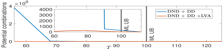
Figure 4: Average potential combinations in MAP with and without LVA for $N=1024$, and $K=8$.

-F Complex Probabilistic Models

In this section, we demonstrate MSGT’s capability to leverage more data when provided with a more complex probabilistic model. To this end, we sample the population based on a Markov process with a 3-time-step memory. We execute MSGT using these prior statistics and also execute it with limited prior statistics, assuming the process has only a 1-time-step memory. The results are shown in Fig. 5. It is evident that utilizing the prior of long memory improves the success probability by $10\%$ in this scenario. We do note again that for the practical regime tested as in [35, 46, 8, 47], i.e., $N=1024$ and $K=8$, it is no longer possible to compare the performance since, unlike the efficient proposed MSGT algorithm, ML and MAP decoders for GT become infeasible.

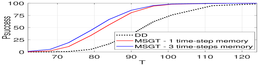
(a) Probability of success in terms of exact recovery.

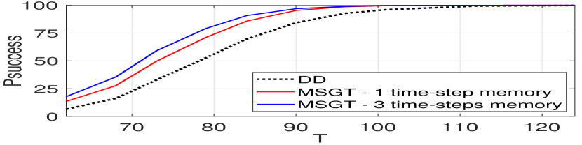
(b) Probability of success in terms of partial recovery

Figure 5: Probability of success of MSGT with exact prior statistics of 3-time-step Markov process, and with limited prior statistics assuming the Markov process has only 1-time-step memory. $N=1024,K=8$, 1000 iterations.

-G Recovery Algorithms

For the completeness of our proposed Algorithm 1, we present here all the algorithms that we use as integral components within MSGT, and provide detailed explanations for each.

-G1 Definitely Not Defective (DND)

DND algorithm [41, 42, 43, 23], which is shown in Algorithm 2 takes the testing matrix $\mathbf{X}$ and the results vector $Y$ as inputs. It systematically compares each column of the $\mathbf{X}$ with $Y^{T}$. If a specific column contains a value of $1$ while its corresponding test result is $0$, we say that this column cannot explain the test result. Since each column represents one item in the population, if $\mathbf{X}(i)$ cannot explain $Y^{T}$, then DND marks this item as definitely non-defective. The output is the list of all the items that were not categorized as definitively non defective, constituting a set we refer to as possibly defective items and denoted by $\mathcal{P}^{(DND)}$.

Algorithm 2 Definite Not Defectives (DND) [41, 42, 43, 23]

Input: $\mathbf{X},Y$
      Output: $\mathcal{P}^{(DND)}$

1:$\mathcal{P}^{(DND)}\leftarrow\left\{1,...,N\right\}$

2:for $i$ s.t. $\mathbf{Y}_{i}=0$ do

3:     for $j$ s.t. $\mathbf{X}_{i,j}=1$ do $\mathcal{P}^{(DND)}\leftarrow\mathcal{P}^{(DND)}\setminus\{j\}$

4:     end for

5:end for

6:return $\mathcal{P}^{(DND)}$

-G2 Definite Defectives (DD)

DD algorithm [23], as shown in Algorithm 3 takes as inputs $\mathcal{P}^{(DND)}$, the testing matrix $\mathbf{X}$ and the results vector $Y$. DD’s objective is to identify test results that can be explained by a single possibly defective item. In practice, DD examines the positive entries of $Y$. For each positive test, if there is only one possibly defective item participating in it, DD marks that item as definitely defective. We skip the last step of DD in [23], and in our implementation, DD returns only the set of definitely defective items, denoted by $\mathcal{D}^{(DD)}$.

Algorithm 3 Definite Defective (DD) [23]

Input: $\mathbf{X},Y,\mathcal{P}^{(DND)}$
      Output: $\mathcal{D}^{(DD)}$

1:$\mathcal{D}^{(DD)}\leftarrow\left\{\right\}$

2:for $i$ s.t. $\mathbf{Y}_{i}=1$ do

3:     for $j\in\mathcal{P}^{(DND)}$ do

4:         if $\mathbf{X}_{i,j}=1$ and $\mathbf{X}_{i,j^{\prime}}=0,$ $\forall j^{\prime}\neq j\in\mathcal{P}^{(DND)}$ then

5:              $\mathcal{D}^{(DD)}\leftarrow\mathcal{D}^{(DD)}\cup\left\{j\right\}$

6:         end if

7:     end for

8:end for

9:return $\mathcal{D}^{(DD)}$

Algorithm 4 List Viterbi Algorithm [33]

Input: $L,\tau,\left\{\mathbf{\pi}_{i}\right\}_{i=1}^{N},\{\mathbf{\Phi}_{i}\}_{i=1}^{N}$
      Output: ${\mathbf{Z}}$

1:Initialization:

2:for $s\leftarrow 1$ to $2^{\tau}$ do

3:     $\Psi(1,s,1)\leftarrow\left\{\mathbf{\pi}_{i}\right\}_{i=1}^{N}\left(s\right)$ $\triangleright$ initial probability for each
                                     state

4:     $\xi\left(n,s,l\right)\leftarrow s$ $\triangleright$ previous state of each state

5:     for $l\leftarrow 2$ to $L$ do

6:         $\Psi(1,s,l)\leftarrow 0$

7:         $\xi\left(n,s,l\right)\leftarrow s$

8:     end for

9:end for

10:Recursion:

11:for $n\leftarrow 2$ to $N$ do

12:     for $s_{2}\leftarrow 1$ to $2^{\tau}$ do

13:         for $l\leftarrow 1$ to $L$ do

14:              $\triangleright$ find the probability of the $l$-most likely
                   previous state and its rank

15:              $\Psi(n,s_{2},l)=\max^{(l)}_{{\begin{subarray}{c}s_{1}\in\{1,...,2^{\tau}\}\\ k\in\{1,..,L\}\end{subarray}}}\newline \hskip 115.00017pt\left\{\Psi(n-1,s_{1},k)\Phi_{n}\left(s_{1},s_{2}\right)\right\}$

16:              $\left({s_{1}}^{*},k^{*}\right)=\arg\max^{(l)}_{{\begin{subarray}{c}s_{1}\in\{1,...,2^{\tau}\}\\ k\in\{1,..,L\}\end{subarray}}}\newline \hskip 115.00017pt\left\{\Psi(n-1,s_{1},k)\Phi_{n}\left(s_{1},s_{2}\right)\right\}$

17:              $\xi\left(n,s_{2},l\right)\leftarrow{s_{1}}^{*}$

18:              $\chi\left(n,l\right)\leftarrow k^{*}$

19:         end for

20:     end for

21:end for

22:Backtracking:

23:for $l\leftarrow 1$ to $L$ do

24:     $\mathbf{Z}_{l,N}\leftarrow\arg\max_{s\in\{1,...,2^{\tau}\}}\left\{\Psi(N,s,l)\right\}$

25:     $l_{N}\leftarrow\chi\left(n,l\right)$

26:     for $n\leftarrow N-1$ to $1$ do

27:         $\mathbf{Z}_{l,n}\leftarrow\xi\left(n+1,\mathbf{Z}_{l_{n+1},n+1},l_{n+1}\right)$

28:         $l_{n}\leftarrow\chi\left(n+1,l_{n+1}\right)$

29:     end for

30:end for

31:return $\mathbf{Z}$

-G3 List Viterbi Algorithm (LVA)

Our variations of the LVA algorithm [33], outlined in Algorithm 4, is designed to return the $L$ most likely sequences, representing the estimation of the whole population, for a given $L\geq 1$. In the algorithm we suggest herein, the key differences are: (1) the population sequence in GT replaces the time sequence in classical LVA as given in [33], and (2) we use the aggregated sequence likelihood instead of the general cost function presented in the original paper. In particular, in the suggested algorithm, as we traverse the trellis diagram, we are iteratively maximizing the likelihood of the sequence representing the status of the population, tested with correlated and non-uniform prior statistics, denoted by $\Psi$ (see line 15).

This algorithm operates in three primary steps: first initialization of the setup, then recursion using a trellis structure to compute probabilities for all possible sequences while eliminating unlikely ones in each step, and finally, backtracking to reconstruct the most probable sequences. The algorithm inputs are the number of the most likely list $L$, the number of memory steps to consider, $\tau$, and the prior statistics $\left\{\mathbf{\pi}_{i}\right\}_{i=1}^{N},\{\mathbf{\Phi}_{i}\}_{i=1}^{N}$.

Let $\Psi\in[0,1]^{N\times 2^{\tau}\times L}$ denote the probabilities of the $L$ most likely states along the trellis. Let $\xi\in\{1,...,2^{\tau}\}^{N\times 2^{\tau}\times L}$ denote the corresponding previous state of each state along the trellis, and let $\chi\in\{1,...,L\}^{N\times 2^{\tau}\times L}$ denote the corresponding rank of the current state, among the $L$ most likely options. In the initialization stage, we fill the given initial probabilities $\left\{\mathbf{\pi}_{i}\right\}_{i=1}^{N}$ in the corresponding entries of $\Psi$, and we set each state to be its previous state (lines 3-4).

In the recursion stage, we iterate from the second item to the last, and for each item, compute all the $2^{\tau}\times 2^{\tau}$ possible transition probabilities between all the possible states he could be in and the states of its predecessor. For each item, state, and rank, we set in $\Psi$ the $L$-most likely probabilities of the overall sequences from the first item until the current item and state (line 15), and we set in $\xi$ the corresponding previous state and in $\chi$ the corresponding rank (lines 17-18). Here, $\max^{(l)}$ denotes the $l$-largest value.

In the backtracking stage, we identify the $L$-most likely sequences based on the probabilities in the entries of the $\Psi$ that correspond to the last item (line 24), and then backtrack the steps of these sequences using the information in $\xi$ (line 27). The algorithm returns a list of these sequences, denoted by $\mathbf{Z}\in\left\{1,...,2^{\tau}\right\}^{L\times N}$. If $\tau>1$, and a further processing is applied to map the states $\{1,...,2^{\tau}\}$ to the binary states $\{0,1\}$, representing ”defective” and ”non-defective”.

-G4 Maximum A Posteriori (MAP)

The MAP estimator [45], as shown in Algorithm 5, returns the set $c\in\mathbf{C}$ with the highest maximum a posteriori probability among all the sets, that is, the set $c$ that obtains the maximum $P\left(Y\lvert\mathbf{X},c\right)P\left(c\right)$. In this expression, the first probability represents the likelihood of obtaining the results $Y$ from a group test using the testing matrix $\mathbf{X}$ and the given set $c$ as the defective set. If the set $c$ and the given testing matrix $\mathbf{X}$ cannot explain for $Y$, then this probability is equal to zero. The second probability corresponds to the prior probability of the overall defective set $c$, calculated using $\left\{\mathbf{\pi}_{i}\right\}_{i=1}^{N},\left\{\mathbf{\Phi}_{i}\right\}_{i=1}^{N}$. The MAP algorithm returns the estimated defective set, denoted by $\hat{\mathcal{K}}$.

Algorithm 5 Maximum A Posteriori (MAP) [45]

Input: $\mathbf{X},Y,\mathbf{C},\left\{\mathbf{\pi}_{i}\right\}_{i=1}^{N},\left\{\mathbf{\Phi}_{i}\right\}_{i=1}^{N}$
      Output: $\hat{\mathcal{K}}$

1:return $\arg\max_{c\in\mathbf{C}}{P\left(Y\lvert\mathbf{X},c\right)P\left(c\right)}$

References

- [1] R. Dorfman, “The detection of defective members of large populations,” The Annals of Mathematical Statistics, vol. 14, no. 4, pp. 436–440, 1943.
- [2] M. T. Thai, Y. Xuan, I. Shin, and T. Znati, “On detection of malicious users using group testing techniques,” in 2008 The 28th Int. Conf. on Distributed Computing Systems. IEEE, 2008, pp. 206–213.
- [3] A. Cohen, A. Cohen, and O. Gurewitz, “Secure group testing,” IEEE Trans. on Inf. Forensics and Security, vol. 16, pp. 4003–4018, 2020.
- [4] A. Cohen, A. Cohen, S. Jaggi, and O. Gurewitz, “Secure adaptive group testing,” in 2018 IEEE Int. Sym. on Inf. Theory (ISIT). IEEE, 2018, pp. 2589–2593.
- [5] P. Indyk, “Deterministic superimposed coding with applications to pattern matching,” in Proceedings 38th Annual Symposium on Foundations of Computer Science. IEEE, 1997, pp. 127–136.
- [6] E. S. Hong and R. E. Ladner, “Group testing for image compression,” IEEE Trans. On image proc., vol. 11, no. 8, pp. 901–911, 2002.
- [7] J. Wolf, “Born again group testing: Multiaccess communications,” IEEE Trans. on Inf. Theory, vol. 31, no. 2, pp. 185–191, 1985.
- [8] A. Cohen, N. Shlezinger, Y. C. Eldar, and M. Médard, “Serial quantization for representing sparse signals,” in 2019 57th Allerton. IEEE, 2019, pp. 987–994.
- [9] P. Nikolopoulos, S. R. Srinivasavaradhan, T. Guo, C. Fragouli, and S. Diggavi, “Community-aware group testing,” IEEE Trans. on Inf. Theory, 2023.
- [10] R. Goenka, S.-J. Cao, C.-W. Wong, A. Rajwade, and D. Baron, “Contact tracing enhances the efficiency of COVID-19 group testing,” in ICASSP 2021-2021 IEEE ICASSP. IEEE, 2021, pp. 8168–8172.
- [11] S. R. Srinivasavaradhan, P. Nikolopoulos, C. Fragouli, and S. Diggavi, “Dynamic group testing to control and monitor disease progression in a population,” in 2022 IEEE Int. Sym. on Inf. Theory (ISIT). IEEE, 2022, pp. 2255–2260.
- [12] A. Cohen, N. Shlezinger, A. Solomon, Y. C. Eldar, and M. Médard, “Multi-level group testing with application to one-shot pooled COVID-19 tests,” in ICASSP 2021-2021 IEEE ICASSP. IEEE, 2021, pp. 1030–1034. Full Version. [Online]. Available: https://drive.google.com/drive/folders/1k77uIgOFXDwmNPdtd72v2IrEnOBgjgud?usp=drive_link
- [13] Y. C. Eldar and G. Kutyniok, “Theory and applications, compressed sensing,” 2012.
- [14] A. C. Gilbert, M. A. Iwen, and M. J. Strauss, “Group testing and sparse signal recovery,” in 2008 42nd Asilomar Conference on Signals, Systems and Computers. IEEE, 2008, pp. 1059–1063.
- [15] V. Y. Tan and G. K. Atia, “Strong impossibility results for sparse signal processing,” IEEE Sig. Proc, Letters, vol. 21, no. 3, pp. 260–264, 2014.
- [16] C. Aksoylar, G. K. Atia, and V. Saligrama, “Sparse signal processing with linear and nonlinear observations: A unified shannon-theoretic approach,” IEEE Trans. on Inf. Theory, vol. 63, no. 2, 2016.
- [17] A. Naderi and Y. Plan, “Sparsity-free compressed sensing with applications to generative priors,” IEEE Journal on Selected Areas in Information Theory, vol. 3, no. 3, pp. 493–501, 2022.
- [18] M. Aldridge, O. Johnson, J. Scarlett et al., “Group testing: an information theory perspective,” Foundations and Trends® in Communications and Information Theory, vol. 15, no. 3-4, pp. 196–392, 2019.
- [19] A. Cohen, A. Cohen, and O. Gurewitz, “Efficient data collection over multiple access wireless sensors network,” IEEE/ACM Transactions on Networking, vol. 28, no. 2, pp. 491–504, 2020.
- [20] A. Cohen, N. Shlezinger, S. Salamatian, Y. C. Eldar, and M. Médard, “Distributed quantization for sparse time sequences,” in 2020 IEEE ICASSP. IEEE, 2020, pp. 5580–5584.
- [21] ——, “Serial quantization for sparse time sequences,” IEEE Transactions on Signal Processing, vol. 69, pp. 3299–3314, 2021.
- [22] G. K. Atia and V. Saligrama, “Boolean compressed sensing and noisy group testing,” IEEE Trans. on Inf. Theory, vol. 58, no. 3, 2012.
- [23] M. Aldridge, L. Baldassini, and O. Johnson, “Group testing algorithms: Bounds and simulations,” IEEE Trans. on Inf. Theory, vol. 60, no. 6, pp. 3671–3687, 2014.
- [24] P. Nikolopoulos, S. R. Srinivasavaradhan, C. Fragouli, and S. N. Diggavi, “Group testing for community infections,” IEEE BITS the Information Theory Magazine, vol. 1, no. 1, pp. 57–68, 2021.
- [25] S. Ahn, W.-N. Chen, and A. Özgür, “Noisy adaptive group testing for community-oriented models,” in 2023 IEEE Int. Sym. on Inf. Theory (ISIT), 2023, pp. 1621–1626.
- [26] ——, “Adaptive group testing on networks with community structure: The stochastic block model,” IEEE Trans. on Inf. Theory, vol. 69, no. 7, pp. 4758–4776, 2023.
- [27] Z. Zhang and B. D. Rao, “Sparse signal recovery with temporally correlated source vectors using sparse bayesian learning,” IEEE Journal of Selected Topics in Signal Processing, vol. 5, no. 5, pp. 912–926, 2011.
- [28] Y. Arjoune, N. Kaabouch, H. El Ghazi, and A. Tamtaoui, “Compressive sensing: Performance comparison of sparse recovery algorithms,” in 2017 IEEE 7th Annual Computing and Communication Workshop and Conference (CCWC), 2017, pp. 1–7.
- [29] B. Arasli and S. Ulukus, “Group testing with a graph infection spread model,” Information, vol. 14, no. 1, p. 48, 2023.
- [30] I. Lau, J. Scarlett, and Y. Sun, “Model-based and graph-based priors for group testing,” arXiv preprint arXiv:2205.11838, 2022.
- [31] J. Andrew, “Viterbi. 1967. error bounds for convolutional codes and an asymptotically optimal decoding algorithm,” IEEE Trans. on Inf. Theory, vol. 13.
- [32] H.-L. Lou, “Implementing the viterbi algorithm,” IEEE Signal processing magazine, vol. 12, no. 5, pp. 42–52, 1995.
- [33] N. Seshadri and C.-E. Sundberg, “List viterbi decoding algorithms with applications,” IEEE Trans. on Comm., vol. 42, no. 234, pp. 313–323, 1994.
- [34] T. K. Moon, Error correction coding: mathematical methods and algorithms. John Wiley & Sons, 2020.
- [35] N. Shental, S. Levy, S. Skorniakov, V. Wuvshet, Y. Shemer-Avni, A. Porgador, and T. Hertz, “Efficient high throughput SARS-CoV-2 testing to detect asymptomatic carriers,” medRxiv, 2020.
- [36] C. Lucia, P.-B. Federico, and G. C. Alejandra, “An ultrasensitive, rapid, and portable coronavirus SARS-CoV-2 sequence detection method based on CRISPR-Cas12,” BioRxiv, pp. 2020–02, 2020.
- [37] I. Yelin, N. Aharony, E. S. Tamar, A. Argoetti, E. Messer, D. Berenbaum, E. Shafran, A. Kuzli, N. Gandali, O. Shkedi et al., “Evaluation of COVID-19 RT-qPCR test in multi sample pools,” Clinical Infectious Diseases, vol. 71, no. 16, pp. 2073–2078, 2020.
- [38] Ben-Ami et al., “Large-scale implementation of pooled RNA extraction and RT-PCR for SARS-CoV-2 detection,” Clinical Microbiology and Infection, vol. 26, no. 9, pp. 1248–1253, 2020.
- [39] O. Johnson, M. Aldridge, and J. Scarlett, “Performance of group testing algorithms with near-constant tests per item,” IEEE Trans. on Inf. Theory, vol. 65, no. 2, pp. 707–723, 2018.
- [40] M. Aldridge, L. Baldassini, and K. Gunderson, “Almost separable matrices,” Jour. of Comb. Opt., vol. 33, pp. 215–236, 2017.
- [41] W. Kautz and R. Singleton, “Nonrandom binary superimposed codes,” IEEE Trans. on Inf. Theory, vol. 10, no. 4, pp. 363–377, 1964.
- [42] H.-B. Chen and F. K. Hwang, “A survey on nonadaptive group testing algorithms through the angle of decoding,” Jour. of Comb. Opt., vol. 15, pp. 49–59, 2008.
- [43] C. L. Chan, P. H. Che, S. Jaggi, and V. Saligrama, “Non-adaptive probabilistic group testing with noisy measurements: Near-optimal bounds with efficient algorithms,” in 2011 49th Allerton. IEEE, 2011, pp. 1832–1839.
- [44] J. Scarlett and V. Cevher, “How little does non-exact recovery help in group testing?” in 2017 IEEE ICASSP. IEEE, 2017, pp. 6090–6094.
- [45] R. G. Gallager, Information theory and reliable communication. Springer, 1968, vol. 588.
- [46] J. Luo and D. Guo, “Neighbor discovery in wireless ad hoc networks based on group testing,” in 2008 46th Annual Allerton Conference on Communication, Control, and Computing. IEEE, 2008, pp. 791–797.
- [47] L. Jacques, K. Degraux, and C. De Vleeschouwer, “Quantized iterative hard thresholding: Bridging 1-bit and high-resolution quantized compressed sensing,” arXiv preprint arXiv:1305.1786, 2013.
- [48] P. Damaschke and A. S. Muhammad, “Competitive group testing and learning hidden vertex covers with minimum adaptivity,” Discrete Mathematics, Algorithms and Applications, vol. 2, no. 03, pp. 291–311, 2010.
- [49] E. N. Gilbert, “Capacity of a burst-noise channel,” Bell system technical journal, vol. 39, no. 5, pp. 1253–1265, 1960.
- [50] Y. Plan and R. Vershynin, “One-bit compressed sensing by linear programming,” Communications on pure and Applied Mathematics, vol. 66, no. 8, pp. 1275–1297, 2013.
- [51] Z. Li, W. Xu, X. Zhang, and J. Lin, “A survey on one-bit compressed sensing: Theory and applications,” Frontiers of Computer Science, vol. 12, pp. 217–230, 2018.
- [52] T. Li, C. L. Chan, W. Huang, T. Kaced, and S. Jaggi, “Group testing with prior statistics,” in 2014 IEEE Int. Sym. on Inf. Theory. IEEE, 2014, pp. 2346–2350.
- [53] S. Bharadwaja, M. Bansal, and C. R. Murthy, “Approximate set identification: Pac analysis for group testing,” in 2022 IEEE Int. Sym. on Inf. Theory (ISIT). IEEE, 2022, pp. 2237–2242.
- [54] J. Kingman, “An introduction to probability theory and its applications,” Journal of the Royal Statistical Society: Series A (General), vol. 135, no. 3, pp. 430–430, 1972.