Unifying Invariance and Spuriousity for Graph Out-of-Distribution via Probability of Necessity and Sufficiency

Abstract.

Graph Out-of-Distribution (OOD), requiring that models trained on biased data generalize to the unseen test data, has a massive of real-world applications. One of the most mainstream methods is to extract the invariant subgraph by aligning the original and augmented data with the help of environment augmentation. However, these solutions might lead to the loss or redundancy of semantic subgraph and further result in suboptimal generalization. To address this challenge, we propose a unified framework to exploit the Probability of Necessity and Sufficiency to extract the Invariant Substructure (PNSIS). Beyond that, this framework further leverages the spurious subgraph to boost the generalization performance in an ensemble manner to enhance the robustness on the noise data. Specificially, we first consider the data generation process for graph data. Under mild conditions, we show that the invariant subgraph can be extracted by minimizing an upper bound, which is built on the theoretical advance of probability of necessity and sufficiency. To further bridge the theory and algorithm, we devise the PNSIS model, which involves an invariant subgraph extractor for invariant graph learning as well invariant and spurious subgraph classifiers for generalization enhancement. Experimental results demonstrate that our PNSIS model outperforms the state-of-the-art techniques on graph OOD on several benchmarks, highlighting the effectiveness in real-world scenarios.

1. Introduction

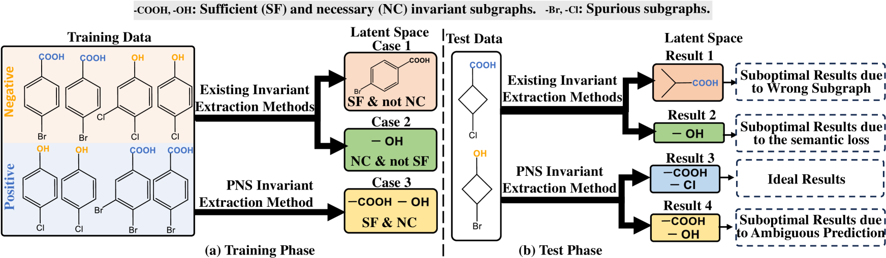
Figure 1. Illustration of graph OOD methods with invariant subgraph learning, (a) In the training phase, the existing invariant extraction methods might lead to sufficient but not necessary subgraphs (pink block) and the necessary but not sufficient subgraphs (green block) according to two extreme optimization goals. The PNS invariant extraction method can extract the correct invariant subgraph. (b) In the test phase, the conventional invariant methods, that extract sufficient but not necessary latent subgraphs, might generate wrong subgraphs and further lead to suboptimal results (pink block). The methods that extract the necessary but not sufficient subgraphs might lead to the loss of semantic information (green block). When the noise-label data exists, the model might generate ambiguous predictions even if the correct subgraphs have been extracted. (yellow block). Ideal performance can be achieved by combining necessary and sufficient invariant subgraphs as well as spurious subgraphs.

Graph representation learning with Graph Neural Networks (GNNs) have gained remarkable success in complicated problems such as social recommendation, intelligent transportation, etc. Despite their enormous success, the existing GNNs generally assume that the testing and training graph data are independently sampled from the identical distribution (I.I.D.). However, the validity of this assumption is often difficult to guarantee in real-world scenarios.

To solve the Out Of Distribution (OOD) challenge of graph data, one of the most popular methods (Li et al., 2022a, b; Zhao et al., 2020; Liu et al., 2023; Sui et al., 2022, 2022) is to extract domain-invariant features for graph data. Previous, Li et al. (Li et al., 2022a) address the OOD challenge by eliminating the statistical dependence between relevant and irrelevant graph representations; Since the spurious correlations lead to the poor generalization of GNNs, Fan et.al (Fan et al., 2023) leverage the stable learning to extract the invariant components. Recently, several researchers have considered the environment-augmentation to extract invariant representation. Liu et.al (Liu et al., 2022a) perform rationale-environment separation to address the graph-ood challenge; Chen et.al (Chen et al., 2023) further use environment augmentation to boost the extraction of invariant features of graph data; And Li (Li et al., 2023b) employ data augmentation techniques to provide identification guarantees for the invariant latent variables. In summary, these methods aim to achieve the invariant representation by balancing two goals 1) aligning the original and augmented feature space and 2) minimizing the prediction error on training data.

Although existing methods with environmental augmentation have achieved outstanding performance in graph OOD, they can hardly extract ideal invariant subgraphs due to the difficulty of the trade-off between invariant alignment and prediction accuracy. To better understand this phenomenon, we provide a toy example of molecular property classification, where the negative and positive labels are decided by special functions like $-\text{COOH}$ and $-\text{OH}$, respectively. Existing methods that balance the feature alignment restriction and the classification loss might result in two extreme cases. As shown in Case 1 of Figure 1(a), when the models put more weight on the optimization of the classification loss, the sufficient but not necessary latent subgraphs are extracted, i.e., the subgraph “Benzene Ring” is involved in the subgraph for classification in the training phase. However, the wrong invariant subgraphs are extracted in the test phase as shown in the pink block of Figure 1(b). Since the invariant subgraphs in the test phase are different from those in the training phase, the model can hardly achieve optimal performance. As shown in Case 2 of Figure 1(a), when there is an overlap between invariant subgraphs of different categories, the model might achieve the necessary but not sufficient latent subgraphs, e.g., the function group “$-$OH”, is shared by “$-$COOH” and “$-$OH”. In this case, the model may fail to distinguish between samples containing “$-$OH” and those containing “$-$COOH”, leading to ambiguous prediction. To solve this problem, the spurious subgraphs, i.e., -Br and -Cl, which are related to the semantic-relevant subgraphs, should be taken into consideration as discussed.

Based on the examples above, an intuitive solution to the graph OOD problem is to 1) extract the sufficient and necessary latent subgraphs and 2) employ the invariant and spurious subgraphs for prediction, which is shown in the blue block of Figure 1(b). Under this intuition, we propose a learning framework to exploit the Probability of Necessity and Sufficiency to extract the Invariant Substructure (PNSIS). Technologically, we first employ the theory of probability of necessity and sufficiency in causality and devise a PNS-invariant subgraph extractor to extract the necessity and sufficiency invariant subgraphs for Graph OOD. Specifically, the PNS-invariant subgraph contains a sufficient subgraph extractor and a necessary subgraph extractor, where the PNS-invariant subgraphs can be extracted by optimizing the PNS upper bound. To further leverage the spurious subgraphs, the proposed PNSIS employs an ensemble train strategy with the spurious subgraphs classifier to introduce the spurious information in the test period. The proposed PNSIS is validated on several mainstream simulated and real-world benchmarks for application evaluation. The impressive performance that outperforms state-of-the-art methods demonstrates the effectiveness of our method.

2. Related Work

2.1. Graph Out-of-Distrubtion.

In this subsection, we provide an introduction to domain generalization of graph classification (Fan et al., 2023; Yang et al., 2022; Guo et al., 2020; Liu et al., 2022a; Chen et al., 2022; Fang et al., 2022). Existing works on out-of-distribution (OOD) (Shen et al., 2021) mainly focus on the fields of computer vision (Zhang et al., 2021, 2022b) and natural language processing (Chen et al., 2021), but the OOD challenge on graph-structured data receives less attention. Considering that the existing GNNs lack out-of-distribution generalization (Li et al., 2022b; Zhao et al., 2020; Liu et al., 2023; Sui et al., 2022; Sun et al., 2022; Li et al., 2022a, 2023b), Li et. al (Li et al., 2021) proposed OOD-GNN to tackle the graph OOD (OOD) challenge by addressing the statistical dependence between relevant and irrelevant graph representations. Recognizing that spurious correlations often undermine the generalization of graph neural networks (GNN), Fan et.al propose the StableGNN (Fan et al., 2023), which extracts causal representation for GNNs with the help of stable learning. Aiming to mitigate the selection bias behind graph-structured data, Wu et. al further proposes the DIR model (Wu et al., 2022) to mine the invariant causal rationales via causal intervention. These methods essentially employ causal effect estimation to make invariant and spurious subgraphs independent. And the augmentation-based model is another type of important method. Liu et.al (Liu et al., 2022b) employ augmentation to improve the robustness and decompose the observed graph into the environment part and the rationale part. Recently, Chen et.al (Chen et al., 2022, 2023) investigate the usefulness of the augmented environment information from the theoretical perspective. And Li et. al (Li et al., 2023b) further consider a concrete scenario of graph OOD, i.e., molecular property prediction from the perspective of latent variables identification (Li et al., 2023a). Although the aforementioned methods mitigate the distribution shift of graph data to some extent, they can not extract the invariant subgraphs with Necessity and Sufficiency (Yang et al., 2023). Moreover, as (Eastwood et al., 2023) discussed, the spurious subgraphs also play a critical role when the data with noisy label (Liu and Tao, 2015; Wu et al., 2024; Bai et al., 2023). In this paper, we propose the PNSIS framework, which unifies the extraction of the invariant latent subgraph with probability of necessity and sufficiency and the exploitation of spurious subgraphs via an ensemble manner.

2.2. Probability of Necessity and Sufficiency

As the probability of causation, the Probability of Necessity and Sufficiency (PNS) can be used to measure the “if and only if” of the relationship between two events. Additionally, the Probability of Necessity (PN) and Probability of Sufficiency (PS) are used to evaluate the “sufficiency cause” and “necessity cause”, respectively. Pearl (Pearl et al., 2000) and Tian and Pearl (Tian and Pearl, 2000) formulated precise meanings for the probabilities of causation using structural causal models. The issue of the identifiability of PNS initially attracted widespread attention (Galles and Pearl, 1998; Halpern, 2000; Pearl, 2009; Cai et al., 2023; Tian and Pearl, 2000; Li and Pearl, 2019, 2022c; Mueller et al., 2021; Dawid et al., 2017; Li and Pearl, 2022b; Gleiss and Schemper, 2019; Zhang et al., 2022a; Li and Pearl, 2022a). Kuroki and Cai [24] and Tian and Pearl [56] demonstrated how to bound these quantities from data obtained in experimental and observational studies to solve this problem. These bounds lie within the range which the probability of causation must lie, however, it has been pointed out that these bounds are too wide to assess the probability of causation. To overcome this difficulty, Pearl demonstrated that identifying the probabilities of causation requires specific functional relationships between the causes and its outcomes (Pearl et al., 2000). Recently, incorporating PNS into various application scenarios has also attracted much attention and currently has many applications (Tan et al., 2022; Galhotra et al., 2021; Watson et al., 2021; Cai et al., 2022; Mueller et al., 2021; Beckers, 2021; Shingaki et al., 2021). For example, in ML explainability, CF² (Tan et al., 2022), LEWIS (Galhotra et al., 2021), LENS (Watson et al., 2021) and NSEG (Cai et al., 2022) use sufficiency or necessity to measure the contribution of input feature subsets to model’s predictions. In the causal effect estimation problem (Mueller et al., 2021; Beckers, 2021; Shingaki et al., 2021), it can be used to learn individual responses from population data (Mueller et al., 2021). In the out-of-distribution generalization problem, CaSN employs PNS to extract domain-invariant information (Yang et al., 2023). Although CaSN is effective in extracting sufficient and necessary invariant representations, it does not capture spurious features that could improve generalization prediction. Therefore, its generalization prediction performance may be suboptimal. Furthermore, the invariant representation learned by CaSN lacks interpretability, while our PNSIS provides interpretable invariant subgraphs.

3. Notations and Problem Formulation

Given the training graphs $\mathcal{G}_{train}=\{(G_{1},Y_{1}),...,$ $(G_{N},Y_{N})\}$, where $G_{n}=(\mathcal{V}_{n},\mathcal{E}_{n},\mathbf{A}_{n})$ represents the $n$-th graph data in the training set and $Y_{n}$ is the corresponding label, with the set of nodes $\mathcal{V}_{n}$, the set of edges $\mathcal{E}_{n}$ and the associated adjacency matrix $\mathbf{A}_{n}\in\mathbb{R}^{|\mathcal{V}_{n}|\times|\mathcal{V}_{n}|}$ where the element of $i$-th row and $j$-th column is 0 if the node pair ($i,j$) has no edges, otherwise it means the edge weight in pair ($i,j$). The node feature matrix of $G_{n}$ is represented as $\mathbf{X}_{n}\in\mathbb{R}^{|\mathcal{V}_{n}|\times D}$, where $i$-th row means the feature of node $i$. We use $\mathbf{B}_{i,:}$ to represent all of the $i$-th row’s elements of a matrix $\mathbf{B}$.

In this paper, we investigate the problem of OOD generalization problem on graph data. We begin with the data generation process as shown in Figure 2, which is known as Partially Informative Invariant Features (PIIF) (Arjovsky et al., 2019). Let $G$ denote an observed graph variable, which is pointed to by $G^{c}$ and $G^{s}$, which means that $G^{c}$ and $G^{s}$ control the generation of the observed graphs. Let $E$ denote the environment indices and $E\to G^{s}$ means that the spurious subgraph in each environment may be different. Remarkably, we find the label $Y$ is the mediator between $G^{c}$ and $G^{s}$, which means that $G^{c}$ and $G^{s}$ is independent given $Y$.

Based on the aforementioned generation process, the task is to learn a GNN model $h_{\varphi}(\cdot)$ with parameter $\varphi$ to accurately predict the label of the testing graphs $\mathcal{G}_{test}$, where the distribution $\Psi(\mathcal{G}_{train})\neq\Psi(\mathcal{G}_{test})$. Note that the test distribution is unknown in the OOD setting. Moreover, we assume the existence of $M$ environments $\{\mathcal{T}_{1},\mathcal{T}_{2},$ $...,\mathcal{T}_{M}\}$ in training graphs $\mathcal{G}_{train}$. For each environment $\mathcal{T}_{i}$, data are drawn from a distinct distribution, represented as $p_{\mathbf{A},\mathbf{X},Y|E_{\mathcal{T}_{i}}}$, where the variables $\mathbf{A}$, $\mathbf{X}$, $Y$ correspond to adjacency matrices, node feature matrices and labels, respectively.

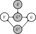
Figure 2. PIIF SCM(Arjovsky et al., 2019). Inside this graph, the noises are omitted for brevity, where the grey and white nodes denote the latent and observed variables, respectively.

4. Invariant Subgraph Learning via PNS Upper Bound Optimization

This section describes a theory for extracting sufficient and necessary invariant subgraphs based on PNS. Specifically, we first introduce the basic model used to build our invariant learning theory. This basic model is a graph generalization model that is jointly predicted by two different invariant subgraph extractors which we call sufficient subgraph extractor and necessary subgraph extractor. Secondly, we reformulate the invariant subgraph learning as a trade-off between the sufficient subgraph extractor and the necessary subgraph extractor. Thirdly, we designed a PNS upper bound that defined on any two different environments for optimization, to enable these two subgraph extractors to produce the necessary and sufficient invariant subgraph.

4.1. Reformulation of Invariant Subgraph Learning via Sufficiency and Necessity

We begin by introducing the basic model that is jointly predicted by two different invariant subgraph extractors and its procedure is broken down into the following three phases. First, feed the same input graph data ($G_{n}$, $Y_{n}$) into two invariant subgraph extractors $f(\cdot;\Theta^{sf})$ and $f(\cdot;\Theta^{nc})$ with parameters given by $\Theta^{sf}$ and $\Theta^{nc}$. $f(\cdot;\Phi^{sf})$ is designed to extract sufficient invariant subgraphs and $f(\cdot;\Phi^{nc})$ is to extract necessary invariant subgraphs, which are called sufficient subgraph extractor and necessary subgraph extractor respectively in this paper (specific details on how to design these two extractors are given in the following sections). Second, feed the output graph from $f(\cdot;\Theta^{sf})$ and $f(\cdot;\Theta^{nc})$ into two different GNNs $g(\cdot;\Phi^{sf})$ and $g(\cdot;\Phi^{nc})$ for classification with parameters given by $\Phi^{sf}$ and $\Phi^{nc}$. Third, average the outputs of the two classifiers and serve as the final prediction. In summary, we formalize the invariant subgraph learning model as follows.

(1) $$\hat{Y}_{n}=0.5\cdot g(f(\mathbf{A}_{n},\mathbf{X}_{n};\Theta^{sf});\Phi^{sf})+0.5\cdot g(f(\mathbf{A}_{n},\mathbf{X}_{n};\Theta^{nc}),\Phi^{nc}),$$

When the outputs of these two subgraph extractors tend to be the same, i.e., their outputs are both sufficient and necessary invariant subgraphs, the prediction accuracy of the model is high. The reasons are as follows. If the sufficient subgraph extractor $f(\cdot;\Theta^{sf})$ captures sufficient but unnecessary invariant subgraph, the prediction may be incorrect since the testing graph may not contain this subgraph. If the necessary subgraph extractor $f(\cdot;\Theta^{nc})$ captures the necessary but insufficient invariant subgraph, the prediction may be also incorrect since other classes of the testing graph may also contain this subgraph. In other words, when the outputs of these two extractors are highly inconsistent, the model’s prediction accuracy will be low. Therefore, the invariant subgraph learning problem is transformed into a trade-off between these two subgraph extractors. In the next section, we describe how to design and optimize this trade-off.

4.2. PNS Upper Bound for Invariant Subgraph Extraction

Probability of Necessity and Sufficiency (PNS) (Pearl, 2022) is to describe the probability that event $A$ occurs if and only if event $B$ occurs. This probability operates in two events to compute the probability that event $A$ is necessary and sufficient cause for event $B$. In this section, we describe a PNS upper bound which is defined on any two different environments for optimization to ensure that the output of the sufficient or necessary subgraph extractor is the necessary and sufficient cause (subgraph format) of the label of the given input graph. To achieve this goal, we first define the PNS risk in a single environment, and then extend its definition to any two environments through upper bound derivation.

4.2.1. PNS Risk.

Let event $A$ denote $G^{c}=f(\mathbf{A}_{n},\mathbf{X}_{n};\Theta^{sf})$ and event $B$ denote $g(f(\mathbf{A}_{n},\mathbf{X}_{n};\Theta^{sf});\Phi^{sf})=y_{n}$. Therefore the occurrence of events $A$ and $B$ means that the prediction of an invariant subgraph generated from $f(\mathbf{A}_{n},\mathbf{X}_{n};\Phi^{sf})$ is the same as the label $y_{n}$. Further, we let $\bar{A}$ denote $G^{c}=f(\mathbf{A}_{n},\mathbf{X}_{n};\Theta^{nc})$ and event $\bar{B}$ denote $g(f(\mathbf{A}_{n},\mathbf{X}_{n};\Theta^{nc});\Phi^{nc})\neq y_{n}$. Thus the occurrence of events $\bar{A}$ and $\bar{B}$ means that the prediction of an invariant subgraph generated from $f(\mathbf{A}_{n},\mathbf{X}_{n};\Phi^{nc})$ is different from the label $y_{n}$. Moreover, the definition of PNS for these events is as follows (Pearl, 2022).

Definition 4.1.

(Probability of necessity, PN)

(2) $$PN=P(\bar{B}_{\bar{A}}|A,B),$$

PN is the probability that, given that events $A$ and $B$ both occur initially, event $B$ does not occur after event $A$ is changed from occurring to not occurring.

Definition 4.2.

(Probability of sufficiency, PS)

(3) $$PS=P({B}_{A}|\bar{A},\bar{B})$$

PS is the probability that, given that events $A$ and $B$ both did not occur initially, event $B$ occurs after event $A$ is changed from not occurring to occurring.

Definition 4.3.

(Probability of necessity and sufficiency, PNS)

(4) $$PNS=PN\cdot P(A,B)+PS\cdot P(\bar{A},\bar{B})$$

PNS is the sum of PN and PS, each multiplied by the probability of its corresponding condition. PNS measures the probability that event $A$ is a necessary and sufficient cause for event $B$.

However, the exact computation of PNS is not tractable in most cases since PN and PS require counterfactual reasoning, and the counterfactual dates are usually difficult to obtain in the real world. We adopt the suggestion proposed by Yang (Yang et al., 2023) and calculate PNS risk based on the observed data in the following way. Let $P(G^{c}|\mathbf{A}_{n},\mathbf{X}_{n};\Theta_{i})$ be a multivariate Bernoulli distribution for invariant subgraph variable $G^{c}$ parameterized by the output of $f(\mathbf{A}_{n},\mathbf{X}_{n};\Theta_{i})$. PNS risk which is defined on environment $E_{\mathcal{T}_{i}}$, is defined as follows.

Definition 4.4.

(PNS risk) The following PNS risk is defined over the distribution of an environment $E_{\mathcal{T}_{i}}$.

(5) $$r^{\mathcal{T}_{i}}_{ns}(\Theta^{sf}, \Phi^{sf},\Theta^{nc},\Phi^{nc}):=\mathbb{E}_{(\mathbf{A}_{n},\mathbf{X}_{n},y_{n})\sim p_{\mathbf{A},\mathbf{X},Y|E_{\mathcal{T}_{i}}}}\big{[}$$

$$\mathbb{E}_{G_{j}^{c}\sim P(G^{c}|\mathbf{A}_{n},\mathbf{X}_{n};\Theta^{sf})}\mathbb{I}[g(G_{j}^{c};\Phi^{sf})\neq y_{n}]$$

$$+\mathbb{E}_{G_{j}^{c}\sim P(G^{c}|\mathbf{A}_{n},\mathbf{X}_{n};\Theta^{nc})}\mathbb{I}[g(G_{j}^{c};\Phi^{nc})=y_{n}]\big{]},$$

PNS risk measures the negative probability that the invariant subgraphs generated by $f(\cdot;\Theta^{sf})$ and $f(\cdot;\Theta^{nc})$ are both the sufficient and necessary cause of $y_{n}$, respectively. To generate the sufficient and necessary invariant subgraph, we extend $r^{\mathcal{T}_{i}}_{ns}(\cdot)$ in Eq. 5 from $E_{\mathcal{T}_{i}}$ to any two environments in the following section.

4.2.2. PNS Upper Bound.

In this section, we propose a graph structure distance to derive an upper bound of the PNS risk. Let $\mathbf{C}_{n}\in\mathbb{R}^{|\mathcal{V}|\times|\mathcal{V}|\times(D+2)}$ be the collection of features of $G_{n}$, where $\mathbf{C}_{n_{:,:,i}}$ ($i\leq D$) denotes the diagonal matrix with diagonal entries being the feature vector of node $i$, $\mathbf{C}_{n_{:,:,D+1}}$ and $\mathbf{C}_{n_{:,:,D+2}}$ represent the adjacency matrix and the euclidean distance matrix between each node feature respectively. Let PMP denote Power-sum Multi-symmetric Polynomials and we use the following permutation invariant function (Maron et al., 2019) which is as powerful as the $3$-WL graph isomorphism test, to encode the structure information of a graph data into a vector.

(6) $$\mathbf{h}_{n}=\sum_{(i_{1},i_{2})\in[V_{n}]^{2}}\mathbf{C}_{n_{i_{1},i_{2},:}}\big{\|}\text{PMP}(\{\kern-3.99994pt\{(\mathbf{C}_{n_{k,i_{2},:}},\mathbf{C}_{n_{i_{1},k,:}})\big{|}k\in[V_{n}]\}\kern-3.99994pt\}),$$

where $\{\kern-3.99994pt\{$ }} represents a multiset, $V_{n}$ is the number of nodes of the graph $G_{n}$, $[V_{n}]=\{1,2,...,V_{n}\}$ and $[V_{n}]^{2}$ denote the Cartesian product of $[V_{n}]$ with itself. Please see Appendix A for more details about this graph structure representation function. After this, let $p_{\mathbf{h}|E_{\mathcal{T}_{i}}}$$(i=1,...,M)$ denote the distribution of graph structure representation in Eq. 6 on different environment data, respectively.

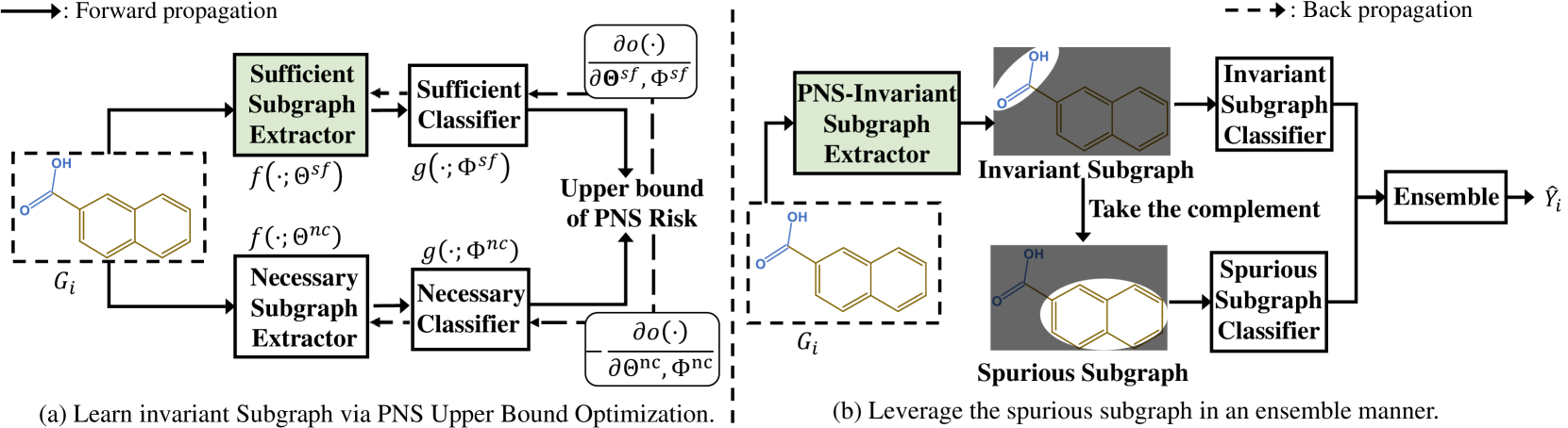
Figure 3. The illustration of the PNSIS framework. (a) The left side of the figure denotes the subgraph extractors that are used to extract the sufficient and necessary invariant subgraphs by optimizing the upper bound. (b) The right side of the figure denotes the ensemble inference phase, which includes an invariant subgraph classifier and a spurious subgraph classifier

We define the graph structure distance as follows.

Definition 4.5.

(Graph Structure Distance, GSD). The structure distance between environments $E_{\mathcal{T}_{i}}$ and $E_{\mathcal{T}_{j}}$ can be formalized as follows:

(7) $$d_{sd}^{\mathcal{T}_{i}\leftrightarrow\mathcal{T}_{j}}(\mathcal{T}_{i}, \mathcal{T}_{j})=dist(p_{\mathbf{h}|E_{\mathcal{T}_{i}}},p_{\mathbf{h}|E_{\mathcal{T}_{j}}})$$

$$+\mathbb{E}_{\mathbf{X}_{i}\sim p_{\mathbf{X}|E_{\mathcal{T}_{i}}}}\big{[}\mathbb{E}_{\mathbf{X}_{j}\sim p_{\mathbf{X}|E_{\mathcal{T}_{j}}}}[\|\mathbf{X}_{i}-\mathbf{X}_{j}\|_{2}]\big{]}$$

Note that $dist(\cdot,\cdot)$ in Eq. 7 can be any distance metric for distribution and we employ the total variation distance in this paper. Hence, our GSD is affected by structure and semantic (node features) information. Moreover, our GSD satisfies the three axioms for a general metric.

Theorem 4.6.

We make the following assumption:

• A1. For any two graphs $G_{i}$, $G_{j}$ from different environments, $G_{i}$ and $G_{j}$ can always be distinguished by the 3-WL graph isomorphism test.

Graph Structure Distance (GSD) satisfies the three axioms for a general metric, to be specific, it satisfies the following conditions:

1. $d_{sd}^{\mathcal{T}_{i}\leftrightarrow\mathcal{T}_{j}}$$\geq$$0$ and $d_{sd}^{\mathcal{T}_{i}\leftrightarrow\mathcal{T}_{j}}$$=$$0$ if and only if $p_{\mathbf{A},\mathbf{X},Y,|E_{\mathcal{T}_{i}}}$$=$$p_{\mathbf{A},\mathbf{X},Y,|E_{\mathcal{T}_{j}}}$;

2. $d_{sd}^{\mathcal{T}_{i}\leftrightarrow\mathcal{T}_{j}}\left(\mathcal{T}_{i},\mathcal{T}_{j}\right)=d_{sd}^{\mathcal{T}_{j}\leftrightarrow\mathcal{T}_{i}}\left(\mathcal{T}_{j},\mathcal{T}_{i}\right)$ (symmetric);

3. $d_{sd}^{\mathcal{T}_{i}\leftrightarrow\mathcal{T}_{j}}\leq d_{sd}^{\mathcal{T}_{i}\leftrightarrow\mathcal{T}_{k}}+d_{SD}^{\mathcal{T}_{k}\leftrightarrow\mathcal{T}_{j}}$ (triangle inequality).

The detailed proof can be found in Appendix C. Next, we provide the upper bound for PNS risk in Eq. 5 through Theorem 4.7.

Theorem 4.7.

(Generalization Bound) We make the following assumption:

• A2: For two distinct environment distributions $p_{\mathbf{A},\mathbf{X},Y,|E_{\mathcal{T}_{i}}}$ and $p_{\mathbf{A},\mathbf{X},Y,|E_{\mathcal{T}_{i}}}$, assume a positive value $K$ exists that satisfies the following inequality:

  (8) $$|p_{\mathbf{A},\mathbf{X},Y|E_{\mathcal{T}_{i}}}-p_{\mathbf{A},\mathbf{X},Y|E_{\mathcal{T}_{j}}}|$$

  $$\leq K\cdot\big{(}|p_{\mathbf{h}|E_{\mathcal{T}_{i}}}-p_{\mathbf{h}|E_{\mathcal{T}_{j}}}|+\mathbb{E}_{\mathbf{X}_{i}\sim p_{\mathbf{X}|E_{\mathcal{T}_{i}}}}\big{[}\mathbb{E}_{\mathbf{X}_{j}\sim p_{\mathbf{X}|E_{\mathcal{T}_{j}}}}[\|\mathbf{X}_{i}-\mathbf{X}_{j}\|_{2}]\big{]}\big{)}$$

  $$= K\cdot d_{sd}^{\mathcal{T}_{i}\leftrightarrow\mathcal{T}_{j}}\left(\mathcal{T}_{i},\mathcal{T}_{j}\right).$$

Based on the aforementioned definition and assumption, we propose the generalization bound for PNS risk in Eq. 5.

(9) $$r^{\mathcal{T}_{i}}_{ns}(\Theta^{sf},\Phi^{sf},\Theta^{nc},\Phi^{nc})\leq r^{\mathcal{T}_{j}}_{ns}(\Theta^{sf},\Phi^{sf},\Theta^{nc},\Phi^{nc})$$

$$+K\cdot\big{(}|p_{\mathbf{h}|E_{\mathcal{T}_{i}}}-p_{\mathbf{h}|E_{\mathcal{T}_{j}}}|+\mathbb{E}_{\mathbf{X}_{i}\sim p_{\mathbf{X}|E_{\mathcal{T}_{i}}}}\big{[}\mathbb{E}_{\mathbf{X}_{j}\sim p_{\mathbf{X}|E_{\mathcal{T}_{j}}}}[\|\mathbf{X}_{i}-\mathbf{X}_{j}\|_{2}]\big{]}\big{)}$$

$$= r^{\mathcal{T}_{j}}_{ns}(\Theta^{sf},\Phi^{sf},\Theta^{nc},\Phi^{nc})+K\cdot d_{sd}^{\mathcal{T}_{i}\leftrightarrow\mathcal{T}_{j}}\left(\mathcal{T}_{i},\mathcal{T}_{j}\right)+\lambda,$$

where $K$, $\lambda$ are constants.

The detailed proof can be found in Appendix D. Finally, combining Eqs. 5, 9, the final objective function $o(\cdot)$ is as follows:

(10) $$\min o(\Theta^{sf},\Theta^{nc},\Phi^{sf},\Phi^{nc})=\mathbb{E}_{(\mathbf{A}_{n},\mathbf{X}_{n},y_{n})\sim p_{\mathbf{A},\mathbf{X},Y|E_{\mathcal{T}_{i}}}}\big{[}$$

$$\mathbb{E}_{G_{j}^{c}\sim P(G^{c}|\mathbf{A}_{n},\mathbf{X}_{n};\Theta^{sf})}\mathbb{I}[g(G_{j}^{c};\Phi^{sf})\neq y_{n}]$$

$$+\mathbb{E}_{G_{j}^{c}\sim P(G^{c}|\mathbf{A}_{n},\mathbf{X}_{n};\Theta^{nc})}\mathbb{I}[g(G_{j}^{c};\Phi^{nc})=y_{n}]\big{]}$$

$$+K\cdot\big{(}|p_{\mathbf{h}|E_{\mathcal{T}_{i}}}-p_{\mathbf{h}|E_{\mathcal{T}_{j}}}|+\mathbb{E}_{\mathbf{X}_{i}\sim p_{\mathbf{X}|E_{\mathcal{T}_{i}}}}\big{[}\mathbb{E}_{\mathbf{X}_{j}\sim p_{\mathbf{X}|E_{\mathcal{T}_{j}}}}[\|\mathbf{X}_{i}-\mathbf{X}_{j}\|_{2}]\big{]}\big{)}.$$

When the objective function in Eq. 10 gradually converges, the output subgraphs of $f(\cdot;\Theta^{sf})$ and $f(\cdot;\Theta^{nc})$ are both necessary and sufficient invariant subgraphs. In practice, we take $f(\cdot;\Theta^{sf})$ and its classifier $g(\cdot;\Phi^{sf})$ as PNS-invariant subgraph extractor and invariant subgraph classifier, respectively. The next section provides a detailed implementation of Eq. 10 and further incorporates spurious features for prediction.

5. Invariant Subgraph Learning Model Incorporating Spurious Subgraph

Building on the theory of invariant subgraph learning via PNS, we exploit the Probability of Necessity and Sufficiency to extract the Invariant Substructure (PNSIS). Beyond that, we further leverage the spurious subgraph to boost the generalization performance in an ensemble manner. The overall framework of PNSIS is shown in Figure 3. Specifically, the procedure of our PNSIS is broken down into the following two phases. In the first phase, PNSIS adopts a stochastic gradient descent algorithm to train sufficient and necessary subgraph extractors to obtain sufficient and necessary invariant subgraphs, as shown in Figure 3 (a). In the second phase, using the trained sufficient subgraph extractor and its classifier as a PNS-invariant subgraph extractor and invariant subgraph classifier, respectively, PNSIS trains a spurious subgraph classifier and integrates the outputs of both classifiers into the final prediction, as shown in Figure 3 (b). More details on the above two phases are given in the following sections.

5.1. Model Implementation and Optimization

In this section, we first provide a concrete implementation of the underlying model in Eq. 1 used to learn sufficient and necessary invariant subgraphs. Second, using Monte Carlo methods to estimate the loss of the model w.r.t the objective function in Eq. 10, and optimize the parameters of the invariant subgraph extractors and classifiers by backpropagation.

5.1.1. Model Implementation.

Technically, we implement the invariant subgraph extractors $f(\mathbf{A}_{n},\mathbf{X}_{n};\Phi^{sf})$ and $f(\mathbf{A}_{n},\mathbf{X}_{n};\Phi^{nc})$, and the subgraph classifiers $g(\cdot;\Phi^{sf})$ and $g(\cdot;\Phi^{nc})$ in the following three steps. First, use two graph convolution networks (GCNs) $\text{GCN}(\mathbf{G};\Theta^{sf})$, $\text{GCN}(\mathbf{G};\Theta^{nc})$ to generate node embeddings $\mathbf{Z}$ and $\mathbf{Z}^{\prime}$, respectively. Second, taking the inner product of $\mathbf{Z}$ and $\mathbf{Z}^{\prime}$ as the output of $f(\cdot;\Theta^{sf})$ and $f(\cdot;\Theta^{nc})$, respectively, where each entry $(i,j)$ in the inner product represents the probability of the edge existence for the node pair $(i,j)$. Third, use another two GCNs $\text{GCN}(\cdot;\Phi^{sf})$ and $\text{GCN}(\cdot;\Phi^{sf})$ as classifiers, respectively. To summarize, the three steps can be formalized as follows.

(11) $$f(\mathbf{A}_{n},\mathbf{X}_{n};\Theta^{sf}):=\sigma(\mathbf{Z}\mathbf{Z}^{\top}),\quad\mathbf{Z}=\text{GCN}(\mathbf{A}_{n},\mathbf{X}_{n};\Theta^{sf}),$$

$$f(\mathbf{A}_{n},\mathbf{X}_{n};\Theta^{nc}):=\sigma(\mathbf{Z}^{\prime}\mathbf{Z}^{\prime\top}),\quad\mathbf{Z}^{\prime}=\text{GCN}(\mathbf{A}_{n},\mathbf{X}_{n};\Theta^{nc}),$$

$$g(f(\cdot;\Theta^{sf});\Phi^{sf}):=\sigma(\text{GCN}(f(\cdot;\Theta^{sf});\Phi^{sf})),$$

$$g(f(\cdot;\Theta^{nc});\Phi^{nc}):=\sigma(\text{GCN}(f(\cdot;\Theta^{nc});\Phi^{nc})),$$

where $\sigma(\cdot)$ is the Sigmoid function.

5.1.2. PNS Upper Bound Estimation.

The objective function in Eq. 10 is estimated as follows. Given a graph dataset $\mathcal{G}_{train}$ and randomly drawn two subsets $\mathcal{G}^{\prime}_{train}$ and $\mathcal{G}^{\prime\prime}_{train}$ from it, which can be regarded as an approximation of a certain two environments $\mathcal{T}_{i}$ and $\mathcal{T}_{j}$ in the training set. First, the last two terms of Eq. 10 can be estimated by $\mathcal{G}^{\prime}_{train}$ and $\mathcal{G}^{\prime\prime}_{train}$. Specifically,

(12) $$|p_{\mathbf{h}|E_{\mathcal{T}_{j}}}-p_{\mathbf{h}|E_{\mathcal{T}_{j}}}|\approx C\cdot\sum^{|\mathcal{G}^{\prime}_{train}|}_{i=1}\sum^{|\mathcal{G}^{\prime\prime}_{train}|}_{j=1}\|\mathbf{h}_{i}-\mathbf{h}_{j}\|_{1},$$

(13) $$\mathbb{E}_{\mathbf{X}_{i}\sim p_{\mathbf{X}|E_{\mathcal{T}_{i}}}}\big{[}\mathbb{E}_{\mathbf{X}_{j}\sim p_{\mathbf{X}|E_{\mathcal{T}_{j}}}}[\|\mathbf{X}_{i}-\mathbf{X}_{j}\|_{2}]\big{]}\approx C\cdot\sum^{|\mathcal{G}^{\prime}_{train}|}_{i=1}\sum^{|\mathcal{G}^{\prime\prime}_{train}|}_{j=1}\|\mathbf{X}_{i}-\mathbf{X}_{j}\|_{2},$$

where $C=1/(|\mathcal{G}^{\prime}_{train}|\cdot|\mathcal{G}^{\prime\prime}_{train}|)$, $\mathbf{X}_{i}$ and $\mathbf{X}_{j}$ are node feature matrices associated with $G_{i}\in\mathcal{G}^{\prime}_{train}$ and $G_{j}\in\mathcal{G}^{\prime\prime}_{train}$ respectively. Secondly, to sample $G^{c}$ from $P(G^{c}|\mathbf{A}_{n},\mathbf{X}_{n};\Theta^{sf})$ and $P(G^{c}|\mathbf{A}_{n},\mathbf{X}_{n};\Theta^{sf})$, we employ Gumbel-Softmax (Jang et al., 2016) and denote the sampling results as $\mathcal{G}_{sf}$ and $\mathcal{G}_{nc}$, respectively. The estimation of Eq. 10 is as follows.

(14) $$\frac{1}{|\mathcal{G}_{train}|}\sum^{|\mathcal{G}_{train}|}_{i=1} \bigg{(}\frac{1}{|\mathcal{G}_{sf}|}\sum^{|\mathcal{G}_{sf}|}_{j=1}\mathbb{I}[g(G_{j}^{c};\Phi^{sf})\neq y_{i}]$$

$$+\frac{1}{|\mathcal{G}_{nc}|}\sum^{|\mathcal{G}_{nc}|}_{k=1}\mathbb{I}[g(G_{k}^{c};\Phi^{nc})=y_{i}]\bigg{)},$$

where $\mathbb{I}[g(G_{j}^{c};\Phi^{sf})$$\neq$$y_{i}]$, $\mathbb{I}[g(G_{j}^{c};\Phi^{sf})$$\neq$$y_{i}]$ can be replaced by other differentiable losses, e.g., cross-entropy loss. Combining Eqs. 12-14, the estimation of PNS upper bound in Eq. 10 is obtained. Finally, PNSIS adopts the SGD algorithm to optimize the estimated PNS upper bound w.r.t. $\Phi^{sf}$, $\Phi^{nc}$, $\Theta^{sf}$ and $\Theta^{nc}$. Due to the opposite training objectives of necessity and sufficiency, this optimization process can be seen as invariant subgraph adversarial learning.

5.2. Fuse Invariant and Spuriousity for Generalization

To enhance the model generalization, we suggest not only making predictions based on their invariant subgraphs but also taking into account their spurious subgraph in the test set. We accomplish this goal in two steps. 1) Build a model to classify testing graphs based on their spurious subgraphs. 2) Ensemble predictions with trained invariant subgraph classifiers. The relevant theories of these steps have been proposed by Eastwood (Eastwood et al., 2023).

5.2.1. Spurious Subgraph Classifier Optimization

Create a pseudo-labelled dataset $\mathcal{G}_{pl}=\{(G^{c}_{n},G^{s}_{n},\hat{Y}_{n})\}^{N}_{n=1}$, where we define a spurious subgraph $G_{n}^{s}$ as the complement of invariant subgraph $G_{n}^{c}$ and $\hat{Y}_{n}$ is the prediction of invariant classifier given $G^{c}_{n}$. Train a graph network classifier $g(\mathbf{A}_{n},\mathbf{X}_{n};\Phi^{sp})$ on this dataset, which we refer to as the spurious subgraph classifier.

5.2.2. Ensemble Prediction

Given $\mathcal{G}_{pl}=$$\{(G^{c}_{n},G^{s}_{n},\hat{Y}_{n})\}^{N}_{n=1}$, trained spurious classifier $g(\cdot;\Phi^{sp})$ and invariant classifier $g(\cdot;\Phi^{sf})$, to simplify the expression, we assume that the OOD task is binary graph classification, and let $\epsilon_{0}=\sum_{\hat{Y}_{n}\in\mathcal{G}_{pl}}\hat{Y}_{n}$, $\epsilon_{1}=\frac{1}{N-\epsilon_{0}}\sum_{n=1}^{N}(1-\hat{Y}_{n})(1-g(G_{n}^{c};\Phi^{sp}))$, $\epsilon_{2}=\frac{1}{\epsilon_{0}}\sum_{n=1}^{N}\hat{Y}_{n}g(G^{c}_{n};\Phi^{sf})$, $\epsilon_{3}=\operatorname{logit}(p(Y=1))$. The ensemble results of the spurious subgraph classifier $g(\cdot;\Phi^{sp})$ and the invariant subgraph classifier $g(\cdot;\Phi^{sf})$ are computed as follows.

(15) $$\hat{Y}=\sigma(\operatorname{logit}(g(G_{n}^{c};\Phi^{sf})))+\operatorname{logit}\Big{(}\frac{g(G^{s}_{n};\Phi^{sp})+\epsilon_{0}-1}{\epsilon_{0}+\epsilon_{1}-1}\Big{)}-\epsilon_{3}.$$

Starting from the leftmost side of Eq. 15, the first three terms can be viewed as $\log p(Y|G^{c},G^{s})$, $\log p(Y|G^{c})$ and $\log p(Y|G^{s})$. Thus the key idea of ensemble prediction (Eastwood et al., 2023) is to decompose $P(Y|G^{c},G^{s})$ into separately estimatable terms. Note that this decomposition holds true if, given $Y$, $G^{c}$ and $G^{s}$ are independent of each other, and the PIIF causal diagram we used in Figure 2 satisfies this condition. See Appendix B for details.

6. Experiments

We evaluate the effectiveness of the proposed PNSIS model on both synthetic and real-world datasets by answering the following questions. Q1: Can the proposed PNSIS model outperforms current state-of-the-art methods under invariant subgraph extraction? Q2: Can the proposed PNS invariant extractor with PNS upper bound restriction well learn the invariant latent subgraphs? Q3: Can the ensemble strategy with spurious subgraphs, which leverages the spurious subgraphs, benefit the model performance?

Table 1. OOD generalization performance on the structure and mixed shifts for synthetic graphs.

	SPMOTIF-STRUC			SPMOTIF-MIXED
Model	BIAS=0.2	BIAS=0.5	BIAS=0.8	BIAS=0.2	BIAS=0.5	BIAS=0.8
ERM	0.5807(0.0225)	0.5998(0.0187)	0.5692(0.0211)	0.5808(0.0198)	0.5725(0.0234)	0.5252(0.0163)
IRM	0.5683(0.0196)	0.5847(0.0203)	0.5327(0.0165)	0.5950(0.0212)	0.5745(0.0186)	0.5488(0.0174)
VREx	0.4343(0.0192)	0.3620(0.0179)	0.3858(0.0186)	0.4453(0.0168)	0.4737(0.0175)	0.3810(0.0162)
GroupDRO	0.5695(0.0171)	0.5782(0.0186)	0.5488(0.0197)	0.5800(0.0164)	0.5782(0.0172)	0.5003(0.0189)
Coral	0.6167(0.0187)	0.6032(0.0174)	0.5288(0.0169)	0.5735(0.0182)	0.5767(0.0191)	0.5292(0.0177)
DANN	0.5767(0.0201)	0.5785(0.0189)	0.5635(0.0222)	0.5682(0.0213)	0.5793(0.0194)	0.5358(0.0178)
Mixup	0.5062(0.0176)	0.5233(0.0191)	0.4965(0.0184)	0.5148(0.0198)	0.5153(0.0167)	0.4988(0.0173)
DIR	0.6237(0.0218)	0.5972(0.0197)	0.5255(0.0176)	0.6435(0.0188)	0.6382(0.0193)	0.4295(0.0169)
GSAT	0.4673(0.0183)	0.4208(0.0215)	0.4152(0.0197)	0.3690(0.0172)	0.4223(0.0168)	0.3688(0.0191)
CIGA	0.601(0.0178)	0.5530(0.0221)	0.5663(0.0182)	0.4982(0.0214)	0.5368(0.0209)	0.5197(0.0187)
CIGAv1	0.5567(0.0195)	0.5047(0.0172)	0.5463(0.0183)	0.5585(0.0197)	0.5400(0.0173)	0.5435(0.0181)
CIGAv2	0.5698(0.0181)	0.5082(0.0164)	0.5122(0.0179)	0.5218(0.0185)	0.4930(0.0188)	0.5180(0.0194)
GALA	0.5976(0.0189)	0.5894(0.0167)	0.5861(0.0178)	0.5833(0.0196)	0.5796(0.0182)	0.5535(0.0175)
PNSIS	0.8113(0.0013)	0.7777(0.0045)	0.7633(0.0121)	0.8128(0.0662)	0.8000(0.0302)	0.7890(0.0025)
ORACLE(IID)	88.70(0.1700)			88.73(0.2500)

Table 2. The ROC-AUC results on seven molecular property classification tasks of the OGB dataset. The values presented are averaged over four replicates with different random seeds. Values in the parenthesis denote the standard errors.

Model	Molhiv	Molbace	Molbbbp	Molclintox	Moltox21	Molsider	Moltoxcast
GCN	0.7580(0.0197)	0.7689(0.0323)	0.6974(0.0153)	0.9027(0.0134)	0.7456(0.0035)	0.5843(0.0034)	0.6421(0.0069)
GAT	0.7652(0.0069)	0.8124(0.0140)	0.6864(0.0298)	0.8798(0.0011)	0.7492(0.0066)	0.5956(0.0102)	0.6466(0.0028)
GraphSAGE	0.7747(0.0115)	0.7425(0.0248)	0.6805(0.0126)	0.8877(0.0066)	0.7410(0.0035)	0.6059(0.0016)	0.6282(0.0067)
GIN	0.7852(0.0158)	0.7638(0.0387)	0.6748(0.0063)	0.9155(0.0212)	0.7440(0.0040)	0.5817(0.0124)	0.6342(0.0102)
GIN0	0.7814(0.0121)	0.7584(0.0239)	0.6611(0.0094)	0.9212(0.0255)	0.7490(0.0015)	0.5968(0.0148)	0.6289(0.0019)
SGC	0.6342(0.0016)	0.6875(0.0021)	0.6613(0.0039)	0.8536(0.0028)	0.7222(0.0005)	0.5906(0.0032)	0.6283(0.0010)
JKNet	0.7534(0.0123)	0.7425(0.0291)	0.6930(0.0075)	0.8558(0.0217)	0.7418(0.0029)	0.5818(0.0159)	0.6357(0.0055)
DIFFPOOL	0.6408(0.0497)	0.7525(0.0116)	0.6935(0.0189)	0.8241(0.0167)	0.7325(0.0084)	0.5758(0.0151)	0.6217(0.0054)
CMPNN	0.7711(0.0071)	0.7215(0.0490)	0.6403(0.0172)	0.7947(0.0461)	0.7048(0.0107)	0.5799(0.0080)	0.6394(0.0105)
DIR	0.7672(0.0084)	0.7834(0.0145)	0.6467(0.0174)	0.8129(0.0307)	0.6966(0.0286)	0.5794(0.0111)	0.6196(0.0135)
StableGNN	0.7779(0.0119)	07695(0.0327)	0.6882(0.0387)	0.8798(0.0237)	0.7312(0.0034)	0.5915(0.0117)	0.6329(0.0069)
AttentiveFP	0.7780(0.0195)	0.7767(0.0026)	0.6555(0.0128)	0.8335(0.0216)	0.7934(0.0028)	0.6919(0.0148)	0.7678(0.0037)
OOD-GNN	0.7950(0.0080)	0.8130(0.0120)	0.7010(0.0100)	0.9140(0.0130)	0.7840(0.0800)	0.6400(0.0130)	0.7870(0.0030)
GIL	0.7908(0.0054)	/	/	/	/	0.6350(0.0057)	/
GREA	0.7932(0.0092)	0.8237(0.0237)	0.6970(0.0128)	0.8789(0.0368)	0.7723(0.0119)	0.6014(0.0204)	0.6732(0.0092)
GALA	0.7788(0.0044)	0.7893(0.0037)	0.6557(0.0335)	0.8737(0.0189)	0.7360(0.0053)	0.5894(0.0051)	0.6297(0.0235)
PNSIS	0.7953(0.0119)	0.8314(0.0181)	0.7040(0.0123)	0.9323(0.0042)	0.7966(0.0023)	0.7278(0.0120)	0.7900(0.0006)

6.1. Setup

6.1.1. Dataset Description

We take the graph generalization in the graph classification task into account and consider synthetic and real-world graph datasets with different distribution shifts to evaluate the performance of PNSIS.

SPMotif datasets. For the simulation dataset, we consider the SPMotif datasets introduced in DIR (Wu et al., 2022), where artificial structural shifts and graph size shifts are nested (SPMotif-Struc). To generate different levels of domain shift, we employ the same simulation method in (Chen et al., 2022) the bias based on fully informative invariant feature (FIIF), where the motif and one of the three base graphs (Tree, Ladder, Wheel) are artificially (spuriously) correlated with a probability of various biases. Furthermore, we also construct a more challenging simulation dataset named SPMotif-Mixed like(Chen et al., 2022), where the node features are spuriously correlated with a probability of different biases by a fixed number of the corresponding labels.

Real-world datasets. To evaluate the proposed PNSIS model in real-world scenarios, we further consider the following real-world datasets. First, we consider seven datasets from the OGBG (Hu et al., 2020) benchmark, which is a collection of realistic and large-scale molecular data. Additionally, we also consider the graph out-of-distribution (GOOD) benchmark dataset (Gui et al., 2022), which is a systematic benchmark for graph out-of-distribution problems. We select four datasets with different split strategies.

All graphs in these datasets are pre-processed using RDKit (Landrum et al., 2006). During preprocessing, these data sets employ a scaffold strategy in the OGBG data set and scaffold/size splitting in the GOOD data set to split molecules based on their two-dimensional structural framework. This preprocessing procedure will inevitably introduce spurious correlations between functional groups due to the selection bias of the training set. Please refer to the Appendix E for the detailed description of the statistics of the dataset.

6.1.2. Baselines

We compare the proposed PNSIS method with two three kinds of baselines. Besides the methods devised for out-of-distribution like ERM (Vedantam et al., 2021), IRM (Arjovsky et al., 2019), VREx (Krueger et al., 2021), GroupDRO (Sagawa et al., 2019), Coral (Sun and Saenko, 2016), DANN (Lempitsky, 2016) and Mixup (Zhang et al., 2017), we also consider the conventional methods based on graph neural networks (GNNs) like GCN (Kipf and Welling, 2016), GAT (Veličković et al., 2017), GraphSage (Hamilton et al., 2017), GIN (Xu et al., 2018a), SGC (Wu et al., 2019), JKNet (Xu et al., 2018b), DIFFPOOL (Ying et al., 2018), CMPNN (Song et al., 2021), AttentiveFP (Xiong et al., 2019), and GSAT (Miao et al., 2022). Then, we further consider the methods that leverage the technique of causal inference like DIR (Wu et al., 2022), StableGNN (Fan et al., 2023), CIGA (Chen et al., 2022), OOD-GNN (Li et al., 2022a). Finally, we consider methods like GALA (Chen et al., 2023), GIL (Li et al., 2022c), and GREA (Liu et al., 2022b), which harness environment augmentation or environment inference to improve generalization. We use ADAM optimizer in all experiments and report the mean accuracy as evaluation metrics. All experiments are implemented by Pytorch on a single NVIDIA RTX A5000 24GB GPU.

Table 3. The AUC-ROC results on four prediction tasks of the GOOD dataset. The values presented are averaged over four replicates with different random seeds. Values in the parenthesis denote the standard errors.

	HIV		Motif		SST2	DrugOOD
Model	scaffold	size	basis	size	length	assay	scaffold	size
ERM	0.6955(0.0239)	0.5919(0.0229)	0.6380(0.1036)	0.5346(0.0408)	0.8052(0.0113)	0.7211(0.0123)	0.6852(0.0145)	0.6465(0.0167)
IRM	0.7017(0.0278)	0.5994(0.0159)	0.5993(11.46)	0.5368(0.0411)	0.8075(0.0117)	0.7076(0.0118)	0.6664(0.0132)	0.6688(0.0146)
VREx	0.6934(0.0354)	0.5849(0.0228)	0.6653(0.0404)	0.5447(0.0342)	0.8020(0.0139)	0.6805(0.0138)	0.6668(0.0150)	0.6768(0.0163)
GroupDRO	0.6815(0.0284)	0.5775(0.0286)	0.6196(0.0827)	0.5169(0.0222)	0.8167(0.0045)	0.7177(0.0122)	0.6897(0.0134)	0.6635(0.0146)
Coral	0.7069(0.0225)	0.5939(0.0290)	0.6623(0.0901)	0.5371(0.0275)	0.7894(0.0122)	0.7181(0.0121)	0.6966(0.0133)	0.6552(0.0145)
DANN	0.6943(0.0242)	0.6238(0.0265)	0.5154(0.0728)	0.5186(0.0244)	0.8053(0.0140)	0.7133(0.0124)	0.6592(0.0136)	0.6627(0.0148)
Mixup	0.7065(0.0186)	0.5911(0.0311)	0.6967(0.0586)	0.5131(0.0256)	0.8077(0.0103)	0.7244(0.0112)	0.6970(0.0124)	0.6648(0.0136)
DIR	0.6844(0.0251)	0.5767(0.0375)	0.3999(0.0550)	0.4483(0.0400)	0.8155(0.0106)	0.6901(0.0143)	0.6420(0.0156)	0.6154(0.0169)
GSAT	0.7007(0.0176)	0.6073(0.0239)	0.5513(0.0541)	0.6076(0.0594)	0.8149(0.0076)	0.6978(0.0137)	0.6450(0.0151)	0.6092(0.0165)
CIGAv1	0.6940(0.0239)	0.6181(0.0168)	0.6643(0.1131)	0.4914(0.0834)	0.8044(0.0124)	0.7089(0.0126)	0.6570(0.0138)	0.6382(0.0152)
CIGAv2	0.6940(0.0197)	0.5955(0.0256)	0.6715(0.0819)	0.5442(0.0311)	0.8046(0.0200)	0.6989(0.0135)	0.6695(0.0147)	0.6410(0.0160)
GALA	0.6864(0.0225)	0.5948(0.0138)	0.6041(0.015)	0.5257(0.0082)	0.7672(0.0136)	0.7101(0.0125)	0.6637(0.0137)	0.6410(0.0159)
PNSIS	0.7167(0.0079)	0.6276(0.0042)	0.7748(0.0221)	0.6326(0.0602)	0.8196(0.0020)	0.7240(0.0113)	0.6991(0.0021)	0.6701(0.0171)

6.1.3. Experiment Results on Simulation Datasets.

The experiment results on the SPMotif simulation datasets are shown in Table 1. Based on the results of the experiment, we can find that the proposed PNSIS method outperforms the other baselines with a large margin in different biases on the standard SPMotif-Struc dataset and the more challenging SPMotif-Mixed dataset. Specifically, the proposed PNISIS achieves more than $25\%$ averaged improvement on all the simulation datasets, indirectly reflecting that our method can extract the invariant subgraphs with the property of necessity and sufficiency. What is more, we also find that the performance drops with increasing biases, showing that overheavy bias can still influence generalization. Moreover, by comparing the variance of different methods, we can find that the variance of the baselines is large, this is because these methods generate the invariant subgraph by trading off two objects, which might lead to unstable results. In the meanwhile, the variance of our method is much smaller, reflecting the stability of our method.

6.1.4. Experiment Results on Real-world Datasets.

The experiment results on the OGBG and GOOD datasets are shown in Table 2 and 3. According to the experiment results, we can draw the following conclusions: 1) the proposed PNSIS outperforms all other baselines on all the datasets, which is attributed to both the PNS restriction for PNS invariant subgraphs and the ensemble training strategy with the help of the spurious subgraphs. 2) Some GNN-based methods such as GCN and GIN do not achieve the ideal performance, reflecting that these methods have limited generalization. 3) The causality-based baselines also achieve comparable performance and the methods based on environmental data-augmentation achieve the closest results, reflecting the usefulness of the environment augmentation. However, since these methods can hardly extract the necessary and sufficient invariant subgraphs, so some experiment results of these methods like Molclintox, Molsider, and Moltoxcast can hardly achieve ideal performance.

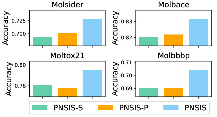
Figure 4. Ablation study on the Molsider, Molbace, Moltox21, and Molbbbp datasets in the OGBG benchmark. We explore the impact of different components in the PNSIS method.

6.2. Ablation Study

To answer Q2 and Q3 to show if the proposed PNS invariant extractor with PNS upper bound restriction and the ensemble strategy with spurious subgraphs benefit the generalization performance, we also devise the two model variants. 1) PNSIS-S: we remove the PNS upper bound restriction from the standard PNSIS. 2) PNSIS-P we remove the ensemble strategy from the standard PNSIS. Experiment results on four datasets in the OBGB benchmark are shown in Figure 4. According to the experiment results, we can find that both the PNS-upper bound restriction and the ensemble strategy play an important role in generalization performance, illustrating the effectiveness of the components in the proposed frameworks.

6.3. Visualization

We further provide visualization of the invariant latent subgraphs extracted by the proposed PNSIS, which is shown in Figure 5. According to the experimental results, we can find that our method can capture the unique atoms of the molecules, i.e. the nitrogen atom and the phosphorus atom, which play a significant role in the molecular property, making it possible to provide inspiration and explanations in the field of chemistry.

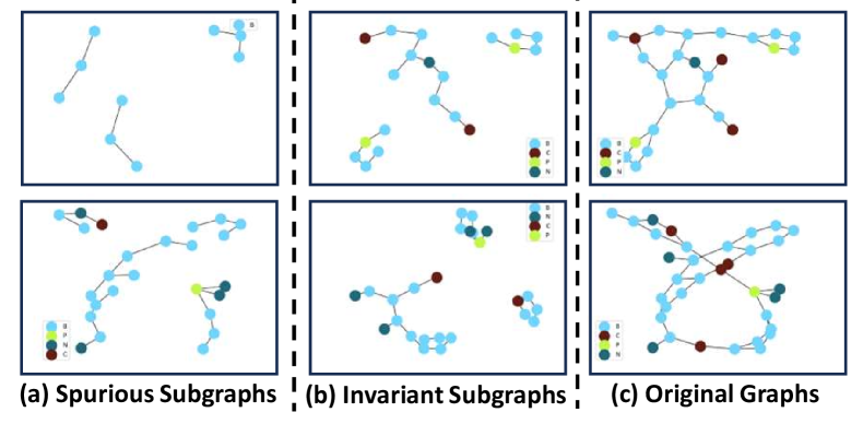
Figure 5. Visualization of molecule examples in the OGBG benchmark. Modes with different colors denote different atoms, and edges denote different chemical bonds.

7. Conclusion

This paper presents a unified framework for graph out-of-distribution, which leverages probability of necessity and sufficiency for invariant subgraph learning and involve spuriousity subgraph for ensemble inference. Based on the conventional data generation process, we prove that the necessity and sufficiency invariant subgraphs can be learned by optimizing the proposed upper bound. By unifying the invariant subgraph extractor and the ensemble inference in the test phase, the proposed PNSIS framework shows outstanding experiment results on the simulation and real-world datasets, highlighting its effectiveness. In summary, this paper takes a meaningful step for the combination of causality and graph representation learning.

Appendix A Background of Power-sum Multi-symmetric Polynomials

Given a graph $G_{n}=(\mathcal{V}_{n},\mathcal{E}_{n},\mathbf{A}_{n})$, use the following permutation-invariant function to get its graph representation $\mathbf{h}_{n}$. This function adopts Power-sum Multi-symmetric Polynomials (PMP) to encode multiset, which is as powerful as the $2$-FWL (equivalent to $3$-WL) graph isomorphism test, as follows.

(16) $$\mathbf{h}_{n}=\sum_{(i_{1},i_{2})\in[V_{n}]^{2}}\mathbf{C}_{n_{i_{1},i_{2},:}}\big{\|}\text{PMP}(\{\kern-3.99994pt\{(\mathbf{C}_{n_{k,i_{2},:}},\mathbf{C}_{n_{i_{1},k,:}})\big{|}k\in[V_{n}]\}\kern-3.99994pt\}),$$

where $\mathbf{C}_{n_{i_{1},i_{2},:}}\in\mathbb{R}^{D}$ is the feature (or color) of $k$-tuple $\bm{i}=(i_{1},i_{2})$.

(17) $$\text{PMP}(\{\kern-3.99994pt\{(\mathbf{C}_{n_{k,i_{2},:}},\mathbf{C}_{n_{i_{1},k,:}})\big{|}k\in[V_{n}]\}\kern-3.99994pt\})=\big{\|}_{j=1}^{D^{\prime}}\mathbf{z}^{j}_{(i_{1},i_{2})},$$

(18) $$\mathbf{z}^{j}_{(i_{1},i_{2})}=\sum_{k\in[V_{n}]}\tau_{1}(\mathbf{C}_{n})_{k,i_{2},j}\odot\tau_{2}(\mathbf{C}_{n})_{i_{1},k,j},$$

where $D^{\prime}=\left(\begin{smallmatrix}N+2D\\ 2D\end{smallmatrix}\right)$, $\tau_{1},\tau_{2}:\mathbb{R}^{D}\to\mathbb{R}^{D\cdot D^{\prime}}$ are two polynomial maps, $\tau_{1}(\mathbf{C}_{n})=\big{\|}_{j=1}^{D^{\prime}}\mathbf{C}_{n}^{\mathbf{a}_{j}}$, $\tau_{2}(\mathbf{C}_{n})=\big{\|}_{j=1}^{D^{\prime}}\mathbf{C}_{n}^{\mathbf{b}_{j}}$, $\mathbf{a}_{j},\mathbf{b}_{j}\in[N]^{D}$, $|\mathbf{a}_{j}|+|\mathbf{b}_{j}|\leq N$, $|\mathbf{a}_{j}|=\sum^{D}_{p=1}a_{jp}$, $[N]=\{1,2,...,N\}$.

Appendix B Formula Derivation for Ensemble Prediction

(19) $$p(Y\mid G^{c},G^{s}) \propto p(G^{c},G^{s}\mid Y)p(Y)$$

$$=p(G^{c}\mid Y)p(G^{s}\mid Y)p(Y)$$

$$\propto\frac{p(Y\mid G^{c})p(Y\mid G^{s})}{p(Y)}$$

The premise for the second line to hold is that given $Y$, then $G^{c}$, and $G^{s}$ are independent of each other.

Appendix C Proof of Theorem 4.6

Proof.

In Definition 4.5, our paper presents the Graph Structure Distance between the source and target domains as shown in Eq. 7. Furthermore, we adopt the total variation distance as the distance metric for the distribution metric. For the graph structure distributions of environments $E_{\mathcal{T}_{i}}$ and $E_{\mathcal{T}_{j}}$, the Graph Structure Distance can be expressed as follows:

(20) $$dist(p_{\mathbf{h}|E_{\mathcal{T}_{i}}},p_{\mathbf{h}|E_{\mathcal{T}_{j}}})$$

$$=TotalVariation(p_{\mathbf{h}|E_{\mathcal{T}_{i}}},p_{\mathbf{h}|E_{\mathcal{T}_{j}}})$$

$$=\frac{1}{2}\sum|p_{\mathbf{h}|E_{\mathcal{T}_{i}}}-p_{\mathbf{h}|E_{\mathcal{T}_{j}}}|$$

(1) Graph Structure Distance satisfies the first axiom: the distance metric function satisfies non-negativity.
From Eq.20, it is easy to see that $|p_{\mathbf{h}|E_{\mathcal{T}_{i}}}-p_{\mathbf{h}|E_{\mathcal{T}_{j}}}|$ is always greater than or equal to 0. And since $\|\mathbf{X}^{i}-\mathbf{X}^{j}\|_{2}$ is always greater than 0, it is proved that the graph structure distance satisfies non-negativity.

(2) Graph Structure Distance satisfies the second axiom: The distance metric function satisfies the commutative property.
From Eq. 20 it can be deduced that $dist(p_{\mathbf{h}|E_{\mathcal{T}_{i}}},p_{\mathbf{h}|E_{\mathcal{T}_{j}}})$ can be expressed as follows:

(21) $$dist(p_{\mathbf{h}|E_{\mathcal{T}_{i}}},p_{\mathbf{h}|E_{\mathcal{T}_{j}}})$$

$$=TotalVariation(p_{\mathbf{h}|E_{\mathcal{T}_{i}}},p_{\mathbf{h}|E_{\mathcal{T}_{j}}})$$

$$=\frac{1}{2}\sum|p_{\mathbf{h}|E_{\mathcal{T}_{i}}}-p_{\mathbf{h}|E_{\mathcal{T}_{j}}}|$$

$$=\frac{1}{2}\sum|p_{\mathbf{h}|E_{\mathcal{T}_{j}}}-p_{\mathbf{h}|E_{\mathcal{T}_{i}}}|$$

$$=TotalVariation(p_{\mathbf{h}|E_{\mathcal{T}_{j}}},p_{\mathbf{h}|E_{\mathcal{T}_{i}}})$$

$$=dist(p_{\mathbf{h}|E_{\mathcal{T}_{j}}},p_{\mathbf{h}|E_{\mathcal{T}_{i}}})$$

For $\mathbb{E}_{\mathbf{X}_{i}\sim p_{\mathbf{X}|E_{\mathcal{T}_{i}}}}\big{[}\mathbb{E}_{\mathbf{X}_{j}\sim p_{\mathbf{X}|E_{\mathcal{T}_{j}}}}[\|\mathbf{X}_{i}-\mathbf{X}_{j}\|_{2}]\big{]}$, we extend it as follows.

(22) $$\mathbb{E}_{\mathbf{X}_{i}\sim p_{\mathbf{X}|E_{\mathcal{T}_{i}}}}\big{[}\mathbb{E}_{\mathbf{X}_{j}\sim p_{\mathbf{X}|E_{\mathcal{T}_{j}}}}[\|\mathbf{X}_{i}-\mathbf{X}_{j}\|_{2}]\big{]}$$

$$=\int\left(\int\|\mathbf{X}_{i}-\mathbf{X}_{j}\|_{2}\,dp_{\mathbf{X}|E_{\mathcal{T}_{j}}}(\mathbf{X}_{j})\right)\,dp_{\mathbf{X}|E_{\mathcal{T}_{i}}}(\mathbf{X}_{i})$$

Next, we use Fubini’s theorem, which allows us to swap the order of integrals, provided the product function is non-negative. Here $\|\mathbf{X}_{i}-\mathbf{X}_{j}\|_{2}$ is non-negative. Therefore, Eq. 23 is supplemented as follows.

(23) $$\mathbb{E}_{\mathbf{X}_{i}\sim p_{\mathbf{X}|E_{\mathcal{T}_{i}}}}\big{[}\mathbb{E}_{\mathbf{X}_{j}\sim p_{\mathbf{X}|E_{\mathcal{T}_{j}}}}[\|\mathbf{X}_{i}-\mathbf{X}_{j}\|_{2}]\big{]}$$

$$=\int\left(\int\|\mathbf{X}_{i}-\mathbf{X}_{j}\|_{2}\,dp_{\mathbf{X}|E_{\mathcal{T}_{j}}}(\mathbf{X}_{j})\right)\,dp_{\mathbf{X}|E_{\mathcal{T}_{i}}}(\mathbf{X}_{i})$$

$$=\int\left(\int\|\mathbf{X}_{i}-\mathbf{X}_{j}\|_{2}\,dp_{\mathbf{X}|E_{\mathcal{T}_{i}}}(\mathbf{X}_{i})\right)\,dp_{\mathbf{X}|E_{\mathcal{T}_{j}}}(\mathbf{X}_{j})$$

$$=\mathbb{E}_{\mathbf{X}_{j}\sim p_{\mathbf{X}|E_{\mathcal{T}_{j}}}}\big{[}\mathbb{E}_{\mathbf{X}_{i}\sim p_{\mathbf{X}|E_{\mathcal{T}_{i}}}}[\|\mathbf{X}_{i}-\mathbf{X}_{j}\|_{2}]\big{]}$$

Therefore, it is proved that the graph structure distance satisfies the commutative property.

(3) Graph Structure Distance (GSD) satisfies the third axiom: The distance metric function satisfies the triangle inequality.

From Eq. 20 it can be deduced that $dist(p_{\mathbf{h}|E_{\mathcal{T}_{i}}},p_{\mathbf{h}|E_{\mathcal{T}_{j}}})$ can be expressed as follows, where $p_{\mathbf{h}|E_{\mathcal{T}_{k}}}$ is an assumed distribution.

(24) $$dist(p_{\mathbf{h}|E_{\mathcal{T}_{i}}},p_{\mathbf{h}|E_{\mathcal{T}_{j}}})=TotalVariation(p_{\mathbf{h}|E_{\mathcal{T}_{i}}},p_{\mathbf{h}|E_{\mathcal{T}_{j}}})$$

$$= \frac{1}{2}\sum|p_{\mathbf{h}|E_{\mathcal{T}_{i}}}-p_{\mathbf{h}|E_{\mathcal{T}_{j}}}|$$

$$= \frac{1}{2}\sum|p_{\mathbf{h}|E_{\mathcal{T}_{i}}}-p_{\mathbf{h}|E_{\mathcal{T}_{k}}}+p_{\mathbf{h}|E_{\mathcal{T}_{k}}}-p_{\mathbf{h}|E_{\mathcal{T}_{j}}}|$$

$$\leq \frac{1}{2}\sum|p_{\mathbf{h}|E_{\mathcal{T}_{i}}}-p_{\mathbf{h}|E_{\mathcal{T}_{k}}}|+\frac{1}{2}\sum|p_{\mathbf{h}|E_{\mathcal{T}_{k}}}-p_{\mathbf{h}|E_{\mathcal{T}_{j}}}|$$

$$= TotalVariation(p_{\mathbf{h}|E_{\mathcal{T}_{i}}},p_{\mathbf{h}|E_{\mathcal{T}_{k}}})+TotalVariation(p_{\mathbf{h}|E_{\mathcal{T}_{k}}},p_{\mathbf{h}|E_{\mathcal{T}_{j}}})$$

$$= dist(p_{\mathbf{h}|E_{\mathcal{T}_{i}}},p_{\mathbf{h}|E_{\mathcal{T}_{k}}})+dict(p_{\mathbf{h}|E_{\mathcal{T}_{k}}},p_{\mathbf{h}|E_{\mathcal{T}_{j}}})$$

In addition, we introduce an auxiliary variable $\mathbf{X}_{k}$ with the distribution $p_{\mathbf{h}|E_{\mathcal{T}_{k}}}$ representing the graph structure representation in domain $E_{\mathcal{T}_{k}}$, and it satisfies $p_{\mathbf{h}|E_{\mathcal{T}_{k}}}(\mathbf{X}_{k},\mathbf{X}_{i})=p_{\mathbf{h}|E_{\mathcal{T}_{k}}}(\mathbf{X}_{k})\cdot p_{\mathbf{h}|E_{\mathcal{T}_{k}}}(\mathbf{X}_{i})$. That is, we introduce a distribution $p_{\mathbf{h}|E_{\mathcal{T}_{k}}}$independent of $p_{\mathbf{h}|E_{\mathcal{T}_{j}}}$ but correlated with $p_{\mathbf{h}|E_{\mathcal{T}_{i}}}$ to construct the auxiliary variable $\mathbf{X}_{k}$. Now, we expand on the expectation part of Eq. 7.

(25) $$\mathbb{E}_{\mathbf{X}_{j}\sim p_{\mathbf{X}|E_{\mathcal{T}_{j}}}}\left[\|\mathbf{X}_{j}-\mathbf{X}_{k}\|_{2}\right]$$

$$=\mathbb{E}_{\mathbf{X}_{j},\mathbf{X}_{k}\sim p_{\mathbf{X}|E_{\mathcal{T}_{j}}}p_{\mathbf{X}|E_{\mathcal{T}_{k}}}}\left[\|\mathbf{X}^{j}-\mathbf{X}^{k}\|_{2}\right]+\mathbb{E}_{\mathbf{X}_{k},\mathbf{X}_{i}\sim p_{\mathbf{X}|E_{\mathcal{T}_{k}}}p_{\mathbf{X}|E_{\mathcal{T}_{i}}}}\left[\|\mathbf{X}_{k}-\mathbf{X}_{i}\|_{2}\right]$$

Next, we apply the basic triangle inequality to Eq. 25.

(26) $$\mathbb{E}_{\mathbf{X}_{j}\sim p_{\mathbf{X}|E_{\mathcal{T}_{j}}}}\left[\|\mathbf{X}_{j}-\mathbf{X}_{k}\|_{2}\right]$$

$$\leq\mathbb{E}_{\mathbf{X}_{j}\sim p_{\mathbf{X}|E_{\mathcal{T}_{j}}}}\left[\|\mathbf{X}_{j}-\mathbf{X}_{k}\|_{2}\right]+\mathbb{E}_{\mathbf{X}_{k}\sim p_{\mathbf{X}|E_{\mathcal{T}_{k}}}}\left[\|\mathbf{X}_{k}-\mathbf{X}_{i}\|_{2}\right]$$

Finally, we can conclude as follows.

(27) $$\mathbb{E}_{\mathbf{X}_{i}\sim p_{\mathbf{X}|E_{\mathcal{T}_{i}}}}\left[E_{\mathbf{X}_{j}\sim p_{\mathbf{X}|E_{\mathcal{T}_{j}}}}\left[\|\mathbf{X}_{j}-\mathbf{X}_{i}\|_{2}\right]\right] \leq\mathbb{E}_{\mathbf{X}_{j}\sim p_{\mathbf{X}|E_{\mathcal{T}_{j}}}}\left[\|\mathbf{X}_{j}-\mathbf{X}_{k}\|_{2}\right]$$

$$+\mathbb{E}_{\mathbf{X}_{k}\sim p_{\mathbf{X}|E_{\mathcal{T}_{k}}}}\left[\|\mathbf{X}_{j}-\mathbf{X}_{k}\|_{2}\right]$$

$$+\mathbb{E}_{\mathbf{X}_{k}\sim p_{\mathbf{X}|E_{\mathcal{T}_{k}}}}\left[\|\mathbf{X}_{k}-\mathbf{X}_{i}\|_{2}\right]$$

Therefore, it is proved that the graph structure distance satisfies the triangle inequality. ∎

Appendix D Proof of Theorem 4.7

Theorem D.1.

(Generalization Bound) We make the following assumption:

• A2: For two distinct environment distributions $p_{\mathbf{A},\mathbf{X},Y,|E_{\mathcal{T}_{i}}}$ and $p_{\mathbf{A},\mathbf{X},Y,|E_{\mathcal{T}_{i}}}$, assume a positive value $K$ exists that satisfies the following inequality:

  (28) $$|p_{\mathbf{A},\mathbf{X},Y,|E_{\mathcal{T}_{i}}}-p_{\mathbf{A},\mathbf{X},Y,|E_{\mathcal{T}_{j}}}|$$

  $$\leq K\cdot\big{(}|p_{\mathbf{h}|E_{\mathcal{T}_{i}}}-p_{\mathbf{h}|E_{\mathcal{T}_{j}}}|+\mathbb{E}_{\mathbf{X}_{i}\sim p_{\mathbf{X}|E_{\mathcal{T}_{i}}}}\big{[}\mathbb{E}_{\mathbf{X}_{j}\sim p_{\mathbf{X}|E_{\mathcal{T}_{j}}}}[\|\mathbf{X}_{i}-\mathbf{X}_{j}\|_{2}]\big{]}\big{)}$$

  $$= K\cdot d_{sd}^{\mathcal{T}_{i}\leftrightarrow\mathcal{T}_{j}}\left(\mathcal{T}_{i},\mathcal{T}_{j}\right).$$

Based on the aforementioned definition and assumption, we propose the generalization bound for PNS risk in Eq. 5.

(29) $$r^{\mathcal{T}_{i}}_{ns}(\Theta^{sf},\Phi^{sf},\Theta^{nc},\Phi^{nc})\leq r^{\mathcal{T}_{j}}_{ns}(\Theta^{sf},\Phi^{sf},\Theta^{nc},\Phi^{nc})$$

$$+K\cdot\big{(}|p_{\mathbf{h}|E_{\mathcal{T}_{i}}}-p_{\mathbf{h}|E_{\mathcal{T}_{j}}}|+\mathbb{E}_{\mathbf{X}_{i}\sim p_{\mathbf{X}|E_{\mathcal{T}_{i}}}}\big{[}\mathbb{E}_{\mathbf{X}_{j}\sim p_{\mathbf{X}|E_{\mathcal{T}_{j}}}}[\|\mathbf{X}_{i}-\mathbf{X}_{j}\|_{2}]\big{]}\big{)}$$

$$= r^{\mathcal{T}_{j}}_{ns}(\Theta^{sf},\Phi^{sf},\Theta^{nc},\Phi^{nc})+K\cdot d_{sd}^{\mathcal{T}_{i}\leftrightarrow\mathcal{T}_{j}}\left(\mathcal{T}_{i},\mathcal{T}_{j}\right)+\lambda,$$

where $K$, $\lambda$ are constants.

Proof.

Let $\eta:\mathcal{A}\times\mathcal{X}\to\{0,1\}$ be the label function. To simplify the description, we overload the symbol $r^{\mathcal{T}_{i}}_{ns}$ in Eq. 5 as a function of input $G_{n}$ and label function $\eta$, as follows.

(30) $$r^{\mathcal{T}_{i}}_{ns}(G_{n},\eta):=\mathbb{E}_{(\mathbf{A}_{n},\mathbf{X}_{n},y_{n})\sim p_{\mathbf{A},\mathbf{X},Y|E_{\mathcal{T}_{i}}}}\big{[}$$

$$\mathbb{E}_{G_{j}^{c}\sim P(G^{c}|\mathbf{A}_{n},\mathbf{X}_{n};\Theta^{sf})}\mathbb{I}[g(G_{j}^{c};\Phi^{sf})\neq\eta(\mathbf{A}_{n},\mathbf{X}_{n})]$$

$$+\mathbb{E}_{G_{j}^{c}\sim P(G^{c}|\mathbf{A}_{n},\mathbf{X}_{n};\Theta^{nc})}\mathbb{I}[g(G_{j}^{c};\Phi^{nc})=\eta(\mathbf{A}_{n},\mathbf{X}_{n})]\big{]}$$

We use the shorthand $r^{\mathcal{T}_{i}}(G_{n})=r^{\mathcal{T}_{i}}_{ns}(G_{n},\eta)$ if the label function defined on the same environment as $r^{\mathcal{T}_{i}}$.

(31) $$r^{\mathcal{T}_{i}}(G_{n})=r^{\mathcal{T}_{i}}(G_{n})+r^{\mathcal{T}_{j}}(G_{n})-r^{\mathcal{T}_{j}}(G_{n})+r^{\mathcal{T}_{j}}(G_{n},\eta^{\mathcal{T}_{i}})-r^{\mathcal{T}_{j}}(G_{n},\eta^{\mathcal{T}_{i}})$$

$$\leq r^{\mathcal{T}_{j}}(G_{n})+r^{\mathcal{T}_{j}}(G_{n},\eta^{\mathcal{T}_{i}})-r^{\mathcal{T}_{j}}(G_{n},\eta^{\mathcal{T}_{j}})+\left|r^{\mathcal{T}_{i}}(G_{n})-r^{\mathcal{T}_{j}}(G_{n},\eta^{\mathcal{T}_{i}})\right|$$

$$\leq r^{\mathcal{T}_{j}}(G_{n})+r^{\mathcal{T}_{j}}(G_{n},\eta^{\mathcal{T}_{i}})+\left|r^{\mathcal{T}_{i}}(G_{n})-r^{\mathcal{T}_{j}}(G_{n},\eta^{\mathcal{T}_{i}})\right|$$

$$\leq r^{\mathcal{T}_{j}}(G_{n})+r^{\mathcal{T}_{j}}(G_{n},\eta^{\mathcal{T}_{i}})+\int|p_{\mathbf{A},\mathbf{X}|E_{\mathcal{T}_{i}}}-p_{\mathbf{A},\mathbf{X}|E_{\mathcal{T}_{i}}}||g_{nc}(f_{nc}(G))$$

$$-\eta^{\mathcal{T}_{i}}(G)|\cdot(1-|g_{sf}(f_{sf}(G))-\eta^{\mathcal{T}_{i}}(G)|)dG$$

$$\leq r^{\mathcal{T}_{j}}(G_{n})+r^{\mathcal{T}_{j}}(G_{n},\eta^{\mathcal{T}_{i}})+\int|p_{\mathbf{A},\mathbf{X}|E_{\mathcal{T}_{i}}}-p_{\mathbf{A},\mathbf{X}}|dG$$

$$\leq r^{\mathcal{T}_{j}}(G_{n})+K\cdot\big{(}|p_{\mathbf{h}|E_{\mathcal{T}_{i}}}-p_{\mathbf{h}|E_{\mathcal{T}_{j}}}|+\mathbb{E}_{\mathbf{X}_{i}\sim p_{\mathbf{X}|E_{\mathcal{T}_{i}}}}\big{[}\mathbb{E}_{\mathbf{X}_{j}\sim p_{\mathbf{X}|E_{\mathcal{T}_{j}}}}[\|\mathbf{X}_{i}-\mathbf{X}_{j}\|_{2}]\big{]}\big{)}$$

$$+\mathbb{E}_{G\sim p_{G|E_{\mathcal{T}_{i}}}}[\eta^{\mathcal{T}_{i}}(G)-\eta^{\mathcal{T}_{j}}(G)]$$

$$= r^{\mathcal{T}_{j}}(G_{n})+K\cdot d^{\mathcal{T}_{i}\leftrightarrow\mathcal{T}_{j}}_{SD}\left(\mathcal{T}_{i},\mathcal{T}_{j}\right)+\lambda,$$

where $\lambda=\epsilon_{S_{i}}\left(\eta_{S_{i}},\eta_{S_{j}}\right)$ is a constant. ∎

Appendix E The Statistics of Datasets

The statistics of the real-world datasets are shown in Table 4.

Table 4. Information about the datasets used in experiments. The number of nodes and edges are taking average among all graphs.

Category	Name	#Graphs	Average #Nodes	Average #Edges	Task Type	Split Method	Metric
OGBG	HIV	41127	25.5	54.9	Binary Classification	scaffold	ROC-AUC
	BACE	1513	34.1	73.7	Binary Classification	scaffold	ROC-AUC
	BBBP	2039	24.1	51.9	Binary Classification	scaffold	ROC-AUC
	ClinTox	1477	26.2	55.8	Binary Classification	scaffold	ROC-AUC
	Tox21	7831	18.6	38.6	Binary Classification	scaffold	ROC-AUC
	SIDER	1427	33.6	70.7	Binary Classification	scaffold	ROC-AUC
	toxcast	8576	18.8	38.5	Binary Classification	scaffold	ROC-AUC
GOOD	hiv	32903	25.3	54.4	Binary Classification	scaffold	ROC-AUC
		32903	24.9	53.6	Binary Classification	size	ROC-AUC
	SST2	44778	10.20	18.40	Binary Classification	Length	ACC
	EC50-Assay	10464	40.89	87.18	Binary Classification	Assay	ROC-AUC
	EC50-Scoffolf	8228	35.54	75.56	Binary Classification	Scoffolf	ROC-AUC
	EC50-Size	10189	35.12	75.30	Binary Classification	Size	ROC-AUC

References

- (1)
- Arjovsky et al. (2019) Martin Arjovsky, Léon Bottou, Ishaan Gulrajani, and David Lopez-Paz. 2019. Invariant risk minimization. arXiv preprint arXiv:1907.02893 (2019).
- Bai et al. (2023) Yingbin Bai, Zhongyi Han, Erkun Yang, Jun Yu, Bo Han, Dadong Wang, and Tongliang Liu. 2023. Subclass-Dominant Label Noise: A Counterexample for the Success of Early Stopping. In Thirty-seventh Conference on Neural Information Processing Systems.
- Beckers (2021) Sander Beckers. 2021. Causal sufficiency and actual causation. Journal of Philosophical Logic 50, 6 (2021), 1341–1374.
- Cai et al. (2023) Hengrui Cai, Yixin Wang, Michael Jordan, and Rui Song. 2023. On learning necessary and sufficient causal graphs. arXiv preprint arXiv:2301.12389 (2023).
- Cai et al. (2022) Ruichu Cai, Yuxuan Zhu, Xuexin Chen, Yuan Fang, Min Wu, Jie Qiao, and Zhifeng Hao. 2022. On the Probability of Necessity and Sufficiency of Explaining Graph Neural Networks: A Lower Bound Optimization Approach. arXiv preprint arXiv:2212.07056 (2022).
- Chen et al. (2021) Jiaao Chen, Dinghan Shen, Weizhu Chen, and Diyi Yang. 2021. Hiddencut: Simple data augmentation for natural language understanding with better generalizability. In Proceedings of the 59th Annual Meeting of the Association for Computational Linguistics and the 11th International Joint Conference on Natural Language Processing (Volume 1: Long Papers). 4380–4390.
- Chen et al. (2023) Yongqiang Chen, Yatao Bian, Kaiwen Zhou, Binghui Xie, Bo Han, and James Cheng. 2023. Does Invariant Graph Learning via Environment Augmentation Learn Invariance? arXiv preprint arXiv:2310.19035 (2023).
- Chen et al. (2022) Yongqiang Chen, Yonggang Zhang, Yatao Bian, Han Yang, MA Kaili, Binghui Xie, Tongliang Liu, Bo Han, and James Cheng. 2022. Learning causally invariant representations for out-of-distribution generalization on graphs. Advances in Neural Information Processing Systems 35 (2022), 22131–22148.
- Dawid et al. (2017) A Philip Dawid, Monica Musio, and Rossella Murtas. 2017. The probability of causation. Law, Probability and Risk 16, 4 (2017), 163–179.
- Eastwood et al. (2023) Cian Eastwood, Shashank Singh, Andrei Liviu Nicolicioiu, Marin Vlastelica, Julius von Kügelgen, and Bernhard Schölkopf. 2023. Spuriosity Didn’t Kill the Classifier: Using Invariant Predictions to Harness Spurious Features. arXiv preprint arXiv:2307.09933 (2023).
- Fan et al. (2023) Shaohua Fan, Xiao Wang, Chuan Shi, Peng Cui, and Bai Wang. 2023. Generalizing graph neural networks on out-of-distribution graphs. IEEE Transactions on Pattern Analysis and Machine Intelligence (2023).
- Fang et al. (2022) Zheng Fang, Ziyun Zhang, Guojie Song, Yingxue Zhang, Dong Li, Jianye Hao, and Xi Wang. 2022. Invariant Factor Graph Neural Networks. In 2022 IEEE International Conference on Data Mining (ICDM). 933–938. https://doi.org/10.1109/ICDM54844.2022.00110
- Galhotra et al. (2021) Sainyam Galhotra, Romila Pradhan, and Babak Salimi. 2021. Explaining black-box algorithms using probabilistic contrastive counterfactuals. In Proceedings of the 2021 International Conference on Management of Data. 577–590.
- Galles and Pearl (1998) David Galles and Judea Pearl. 1998. An axiomatic characterization of causal counterfactuals. Foundations of Science 3 (1998), 151–182.
- Gleiss and Schemper (2019) Andreas Gleiss and Michael Schemper. 2019. Quantifying degrees of necessity and of sufficiency in cause-effect relationships with dichotomous and survival outcomes. Statistics in Medicine 38, 23 (2019), 4733–4748.
- Gui et al. (2022) Shurui Gui, Xiner Li, Limei Wang, and Shuiwang Ji. 2022. Good: A graph out-of-distribution benchmark. Advances in Neural Information Processing Systems 35 (2022), 2059–2073.
- Guo et al. (2020) Zhichun Guo, Wenhao Yu, Chuxu Zhang, Meng Jiang, and Nitesh V Chawla. 2020. GraSeq: graph and sequence fusion learning for molecular property prediction. In Proceedings of the 29th ACM international conference on information & knowledge management. 435–443.
- Halpern (2000) Joseph Y Halpern. 2000. Axiomatizing causal reasoning. Journal of Artificial Intelligence Research 12 (2000), 317–337.
- Hamilton et al. (2017) Will Hamilton, Zhitao Ying, and Jure Leskovec. 2017. Inductive representation learning on large graphs. Advances in neural information processing systems 30 (2017).
- Hu et al. (2020) Weihua Hu, Matthias Fey, Marinka Zitnik, Yuxiao Dong, Hongyu Ren, Bowen Liu, Michele Catasta, and Jure Leskovec. 2020. Open graph benchmark: Datasets for machine learning on graphs. Advances in neural information processing systems 33 (2020), 22118–22133.
- Jang et al. (2016) Eric Jang, Shixiang Gu, and Ben Poole. 2016. Categorical reparameterization with gumbel-softmax. arXiv preprint arXiv:1611.01144 (2016).
- Kipf and Welling (2016) Thomas N Kipf and Max Welling. 2016. Semi-supervised classification with graph convolutional networks. arXiv preprint arXiv:1609.02907 (2016).
- Krueger et al. (2021) David Krueger, Ethan Caballero, Joern-Henrik Jacobsen, Amy Zhang, Jonathan Binas, Dinghuai Zhang, Remi Le Priol, and Aaron Courville. 2021. Out-of-distribution generalization via risk extrapolation (rex). In International Conference on Machine Learning. PMLR, 5815–5826.
- Landrum et al. (2006) Greg Landrum et al. 2006. RDKit: Open-source cheminformatics. (2006).
- Lempitsky (2016) Victor Lempitsky. 2016. Domain-adversarial training of neural networks. The Journal (2016).
- Li and Pearl (2019) Ang Li and Judea Pearl. 2019. Unit selection based on counterfactual logic. In Proceedings of the Twenty-Eighth International Joint Conference on Artificial Intelligence.
- Li and Pearl (2022a) Ang Li and Judea Pearl. 2022a. Bounds on causal effects and application to high dimensional data. In Proceedings of the AAAI Conference on Artificial Intelligence, Vol. 36. 5773–5780.
- Li and Pearl (2022b) Ang Li and Judea Pearl. 2022b. Probabilities of causation with nonbinary treatment and effect. arXiv preprint arXiv:2208.09568 (2022).
- Li and Pearl (2022c) Ang Li and Judea Pearl. 2022c. Unit selection with causal diagram. In Proceedings of the AAAI conference on artificial intelligence, Vol. 36. 5765–5772.
- Li et al. (2021) Haoyang Li, Xin Wang, Ziwei Zhang, and Wenwu Zhu. 2021. Ood-gnn: Out-of-distribution generalized graph neural network. arXiv preprint arXiv:2112.03806 (2021).
- Li et al. (2022a) Haoyang Li, Xin Wang, Ziwei Zhang, and Wenwu Zhu. 2022a. Ood-gnn: Out-of-distribution generalized graph neural network. IEEE Transactions on Knowledge and Data Engineering (2022).
- Li et al. (2022c) Haoyang Li, Ziwei Zhang, Xin Wang, and Wenwu Zhu. 2022c. Learning invariant graph representations for out-of-distribution generalization. Advances in Neural Information Processing Systems 35 (2022), 11828–11841.
- Li et al. (2023a) Zijian Li, Ruichu Cai, Guangyi Chen, Boyang Sun, Zhifeng Hao, and Kun Zhang. 2023a. Subspace Identification for Multi-Source Domain Adaptation. arXiv preprint arXiv:2310.04723 (2023).
- Li et al. (2022b) Zenan Li, Qitian Wu, Fan Nie, and Junchi Yan. 2022b. Graphde: A generative framework for debiased learning and out-of-distribution detection on graphs. Advances in Neural Information Processing Systems 35 (2022), 30277–30290.
- Li et al. (2023b) Zijian Li, Zunhong Xu, Ruichu Cai, Zhenhui Yang, Yuguang Yan, Zhifeng Hao, Guangyi Chen, and Kun Zhang. 2023b. Identifying Semantic Component for Robust Molecular Property Prediction. arXiv preprint arXiv:2311.04837 (2023).
- Liu et al. (2022a) Gang Liu, Tong Zhao, Jiaxin Xu, Tengfei Luo, and Meng Jiang. 2022a. Graph rationalization with environment-based augmentations. In Proceedings of the 28th ACM SIGKDD Conference on Knowledge Discovery and Data Mining. 1069–1078.
- Liu et al. (2022b) Gang Liu, Tong Zhao, Jiaxin Xu, Tengfei Luo, and Meng Jiang. 2022b. Graph Rationalization with Environment-Based Augmentations. In Proceedings of the 28th ACM SIGKDD Conference on Knowledge Discovery and Data Mining (Washington DC, USA) (KDD ’22). Association for Computing Machinery, New York, NY, USA, 1069–1078. https://doi.org/10.1145/3534678.3539347
- Liu and Tao (2015) Tongliang Liu and Dacheng Tao. 2015. Classification with noisy labels by importance reweighting. IEEE Transactions on pattern analysis and machine intelligence 38, 3 (2015), 447–461.
- Liu et al. (2023) Yang Liu, Xiang Ao, Fuli Feng, Yunshan Ma, Kuan Li, Tat-Seng Chua, and Qing He. 2023. FLOOD: A Flexible Invariant Learning Framework for Out-of-Distribution Generalization on Graphs. In Proceedings of the 29th ACM SIGKDD Conference on Knowledge Discovery and Data Mining. 1548–1558.
- Maron et al. (2019) Haggai Maron, Heli Ben-Hamu, Hadar Serviansky, and Yaron Lipman. 2019. Provably powerful graph networks. Advances in neural information processing systems 32 (2019).
- Miao et al. (2022) Siqi Miao, Mia Liu, and Pan Li. 2022. Interpretable and generalizable graph learning via stochastic attention mechanism. In International Conference on Machine Learning. PMLR, 15524–15543.
- Mueller et al. (2021) Scott Mueller, Ang Li, and Judea Pearl. 2021. Causes of effects: Learning individual responses from population data. arXiv preprint arXiv:2104.13730 (2021).
- Pearl (2009) Judea Pearl. 2009. Causality. Cambridge university press.
- Pearl (2022) Judea Pearl. 2022. Probabilities of causation: three counterfactual interpretations and their identification. In Probabilistic and Causal Inference: The Works of Judea Pearl. 317–372.
- Pearl et al. (2000) Judea Pearl et al. 2000. Models, reasoning and inference. Cambridge, UK: CambridgeUniversityPress 19, 2 (2000), 3.
- Sagawa et al. (2019) Shiori Sagawa, Pang Wei Koh, Tatsunori B Hashimoto, and Percy Liang. 2019. Distributionally robust neural networks for group shifts: On the importance of regularization for worst-case generalization. arXiv preprint arXiv:1911.08731 (2019).
- Shen et al. (2021) Zheyan Shen, Jiashuo Liu, Yue He, Xingxuan Zhang, Renzhe Xu, Han Yu, and Peng Cui. 2021. Towards out-of-distribution generalization: A survey. arXiv preprint arXiv:2108.13624 (2021).
- Shingaki et al. (2021) Ryusei Shingaki et al. 2021. Identification and estimation of joint probabilities of potential outcomes in observational studies with covariate information. Advances in Neural Information Processing Systems 34 (2021), 26475–26486.
- Song et al. (2021) Ying Song, Shuangjia Zheng, Zhangming Niu, Zhang-Hua Fu, Yutong Lu, and Yuedong Yang. 2021. Communicative Representation Learning on Attributed Molecular Graphs. In Proceedings of the Twenty-Ninth International Joint Conference on Artificial Intelligence (Yokohama, Yokohama, Japan) (IJCAI’20). Article 392, 8 pages.
- Sui et al. (2022) Yongduo Sui, Xiang Wang, Jiancan Wu, Min Lin, Xiangnan He, and Tat-Seng Chua. 2022. Causal attention for interpretable and generalizable graph classification. In Proceedings of the 28th ACM SIGKDD Conference on Knowledge Discovery and Data Mining. 1696–1705.
- Sun and Saenko (2016) Baochen Sun and Kate Saenko. 2016. Deep coral: Correlation alignment for deep domain adaptation. In Computer Vision–ECCV 2016 Workshops: Amsterdam, The Netherlands, October 8-10 and 15-16, 2016, Proceedings, Part III 14. Springer, 443–450.
- Sun et al. (2022) Ruoxi Sun, Hanjun Dai, and Adams Wei Yu. 2022. Does GNN Pretraining Help Molecular Representation? Advances in Neural Information Processing Systems 35 (2022), 12096–12109.
- Tan et al. (2022) Juntao Tan, Shijie Geng, Zuohui Fu, Yingqiang Ge, Shuyuan Xu, Yunqi Li, and Yongfeng Zhang. 2022. Learning and evaluating graph neural network explanations based on counterfactual and factual reasoning. In Proceedings of the ACM Web Conference 2022. 1018–1027.
- Tian and Pearl (2000) Jin Tian and Judea Pearl. 2000. Probabilities of causation: Bounds and identification. Annals of Mathematics and Artificial Intelligence 28, 1-4 (2000), 287–313.
- Vedantam et al. (2021) Ramakrishna Vedantam, David Lopez-Paz, and David J Schwab. 2021. An empirical investigation of domain generalization with empirical risk minimizers. Advances in Neural Information Processing Systems 34 (2021), 28131–28143.
- Veličković et al. (2017) Petar Veličković, Guillem Cucurull, Arantxa Casanova, Adriana Romero, Pietro Lio, and Yoshua Bengio. 2017. Graph attention networks. arXiv preprint arXiv:1710.10903 (2017).
- Watson et al. (2021) David S Watson, Limor Gultchin, Ankur Taly, and Luciano Floridi. 2021. Local explanations via necessity and sufficiency: Unifying theory and practice. In Uncertainty in Artificial Intelligence. PMLR, 1382–1392.
- Wu et al. (2019) Felix Wu, Amauri Souza, Tianyi Zhang, Christopher Fifty, Tao Yu, and Kilian Weinberger. 2019. Simplifying graph convolutional networks. In International conference on machine learning. PMLR, 6861–6871.
- Wu et al. (2024) Songhua Wu, Tianyi Zhou, Yuxuan Du, Jun Yu, Bo Han, and Tongliang Liu. 2024. A Time-Consistency Curriculum for Learning from Instance-Dependent Noisy Labels. IEEE Transactions on Pattern Analysis and Machine Intelligence (2024).
- Wu et al. (2022) Ying-Xin Wu, Xiang Wang, An Zhang, Xiangnan He, and Tat-Seng Chua. 2022. Discovering invariant rationales for graph neural networks. arXiv preprint arXiv:2201.12872 (2022).
- Xiong et al. (2019) Zhaoping Xiong, Dingyan Wang, Xiaohong Liu, Feisheng Zhong, Xiaozhe Wan, Xutong Li, Zhaojun Li, Xiaomin Luo, Kaixian Chen, Hualiang Jiang, et al. 2019. Pushing the boundaries of molecular representation for drug discovery with the graph attention mechanism. Journal of medicinal chemistry 63, 16 (2019), 8749–8760.
- Xu et al. (2018a) Keyulu Xu, Weihua Hu, Jure Leskovec, and Stefanie Jegelka. 2018a. How powerful are graph neural networks? arXiv preprint arXiv:1810.00826 (2018).
- Xu et al. (2018b) Keyulu Xu, Chengtao Li, Yonglong Tian, Tomohiro Sonobe, Ken-ichi Kawarabayashi, and Stefanie Jegelka. 2018b. Representation learning on graphs with jumping knowledge networks. In International conference on machine learning. PMLR, 5453–5462.
- Yang et al. (2023) Mengyue Yang, Zhen Fang, Yonggang Zhang, Yali Du, Furui Liu, Jean-Francois Ton, and Jun Wang. 2023. Invariant Learning via Probability of Sufficient and Necessary Causes. arXiv preprint arXiv:2309.12559 (2023).
- Yang et al. (2022) Nianzu Yang, Kaipeng Zeng, Qitian Wu, Xiaosong Jia, and Junchi Yan. 2022. Learning substructure invariance for out-of-distribution molecular representations. Advances in Neural Information Processing Systems 35 (2022), 12964–12978.
- Ying et al. (2018) Zhitao Ying, Jiaxuan You, Christopher Morris, Xiang Ren, Will Hamilton, and Jure Leskovec. 2018. Hierarchical graph representation learning with differentiable pooling. Advances in neural information processing systems 31 (2018).
- Zhang et al. (2017) Hongyi Zhang, Moustapha Cisse, Yann N Dauphin, and David Lopez-Paz. 2017. mixup: Beyond empirical risk minimization. arXiv preprint arXiv:1710.09412 (2017).
- Zhang et al. (2022a) Junzhe Zhang, Jin Tian, and Elias Bareinboim. 2022a. Partial counterfactual identification from observational and experimental data. In International Conference on Machine Learning. PMLR, 26548–26558.
- Zhang et al. (2022b) Weijia Zhang, Xuanhui Zhang, Min-Ling Zhang, et al. 2022b. Multi-instance causal representation learning for instance label prediction and out-of-distribution generalization. Advances in Neural Information Processing Systems 35 (2022), 34940–34953.
- Zhang et al. (2021) Xingxuan Zhang, Peng Cui, Renzhe Xu, Linjun Zhou, Yue He, and Zheyan Shen. 2021. Deep stable learning for out-of-distribution generalization. In Proceedings of the IEEE/CVF Conference on Computer Vision and Pattern Recognition. 5372–5382.
- Zhao et al. (2020) Xujiang Zhao, Feng Chen, Shu Hu, and Jin-Hee Cho. 2020. Uncertainty aware semi-supervised learning on graph data. Advances in Neural Information Processing Systems 33 (2020), 12827–12836.