Less is More: Fewer Interpretable Region via Submodular Subset Selection

Abstract

Image attribution algorithms aim to identify important regions that are highly relevant to model decisions. Although existing attribution solutions can effectively assign importance to target elements, they still face the following challenges: 1) existing attribution methods generate inaccurate small regions thus misleading the direction of correct attribution, and 2) the model cannot produce good attribution results for samples with wrong predictions. To address the above challenges, this paper re-models the above image attribution problem as a submodular subset selection problem, aiming to enhance model interpretability using fewer regions. To address the lack of attention to local regions, we construct a novel submodular function to discover more accurate small interpretation regions. To enhance the attribution effect for all samples, we also impose four different constraints on the selection of sub-regions, i.e., confidence, effectiveness, consistency, and collaboration scores, to assess the importance of various subsets. Moreover, our theoretical analysis substantiates that the proposed function is in fact submodular. Extensive experiments show that the proposed method outperforms SOTA methods on two face datasets (Celeb-A and VGG-Face2) and one fine-grained dataset (CUB-200-2011). For correctly predicted samples, the proposed method improves the Deletion and Insertion scores with an average of 4.9% and 2.5% gain relative to HSIC-Attribution. For incorrectly predicted samples, our method achieves gains of 81.0% and 18.4% compared to the HSIC-Attribution algorithm in the average highest confidence and Insertion score respectively. The code is released at https://github.com/RuoyuChen10/SMDL-Attribution.

1 Introduction

Building transparent and explainable artificial intelligence (XAI) models is crucial for humans to reasonably and effectively exploit artificial intelligence (Dwivedi et al., 2023; Ya et al., 2024; Li et al., 2021b; Tu et al., 2023; Liang et al., 2022a; b; 2023b). Solving the interpretability and security problems of AI has become an urgent challenge in the current field of AI research (Arrieta et al., 2020; Chen et al., 2023; Zhao et al., 2023; Liang et al., 2023a; 2024; Li et al., 2023). Image attribution algorithms are typical interpretable methods, which produce saliency maps that explain which image regions are more important to model decisions. It provides a deeper understanding of the operating mechanisms of deep models, aids in identifying sources of prediction errors, and contributes to model improvement. Image attribution algorithms encompass two primary categories: white-box methods (Chattopadhay et al., 2018; Wang et al., 2020) chiefly attribute on the basis of the model’s internal characteristics or decision gradients, and black-box methods (Petsiuk et al., 2018; Novello et al., 2022), which primarily analyze the significance of input regions via external perturbations.

Although attribution algorithms have been well studied, they still face two following limitations: 1) Some attribution regions are not small and dense enough which may interfere with the optimization orientation. Most advanced attribution algorithms focus on understanding how the global image contributes to the prediction results of the deep model while ignoring the impact of local regions on the results. 2) It is difficult to effectively attribute the latent cause of the error to samples with incorrect predictions. For incorrectly predicted samples, although the attribution algorithm can assign the correct class, it does not limit the response to the incorrect class, so that the attributed region may still have a high response to the incorrect class.

To solve the above issues, we propose a novel explainable method that reformulates the attribution problem as a submodular subset selection problem. We hypothesize that local regions can achieve better interpretability, and hope to achieve higher interpretability with fewer regions. We first divide the image into multiple sub-regions and achieve attribution by selecting a fixed number of sub-regions to achieve the best interpretability. To alleviate the insufficient dense of the attribution region, we employ regional search to continuously expand the sub-region set. Furthermore, we introduce a new attribution mechanism to excavate what regions promote interpretability from four aspects, i.e., the prediction confidence of the model, the effectiveness of regional semantics, the consistency of semantics, and the collective effect of the region. Based on these useful clues, we design a submodular function to evaluate the significance of various subsets, which can limit the search for regions with wrong class responses. As shown in Fig. 1, we find that for correctly predicted samples, the proposed method can obtain higher prediction confidence with only a few regions as input than with all regions as input, and for incorrectly predicted samples, our method has the ability to find the reasons (e.g., the dark background region) that caused its prediction error.

We validate the effectiveness of our method on two face datasets, i.e., Celeb-A (Liu et al., 2015), VGG-Face2 (Cao et al., 2018), and a fine-grained dataset CUB-200-2011 (Welinder et al., 2010). For correctly predicted samples, compared with the SOTA method HSIC-Attribution (Novello et al., 2022), our method improves the Deletion scores by 8.4%, 1.0%, and 5.3%, and the Insertion scores by 1.1%, 0.2%, and 6.1%, respectively. For incorrectly predicted samples, our method excels in identifying the reasons behind the model’s decision-making errors. In particular, compared with the SOTA method HSIC-Attribution, the average highest confidence is increased by 81.0%, and the Insertion score is increased by 18.4% on the CUB-200-2011 dataset. Furthermore, our analysis at the theoretical level confirms that the proposed function is indeed submodular. Please see Appendix 5 for a list of important notations employed in this article.

Our contributions can be summarized as follows:

• We reformulate the attribution problem as a submodular subset selection problem that achieves higher interpretability with fewer dense regions.

• A novel submodular mechanism is constructed to evaluate the significance of various subsets from four different aspects, i.e., the confidence, effectiveness, consistency, and collaboration scores. It not only improves the dense of attribution regions for existing attribution algorithms but also better discovers the causes of image prediction errors.

• The proposed method has good versatility which can improve the interpretability of both on the face and fine-grained datasets. Experimental results show that it can achieve better attribution results for the correctly predicted samples and effectively discover the causes of model prediction errors for incorrectly predicted samples.

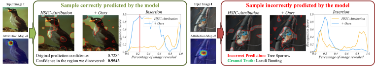
Figure 1: For correctly predicted samples, our method can find fewer regions that make the model predictions more confident. For incorrectly predicted samples, our method can find the reasons that caused the model to predict incorrectly.

2 Related Work

White-Box Attribution Method

Image attribution algorithms are designed to ascertain the importance of different input regions within an image with respect to the decision-making process of the model. White-box attribution algorithms primarily rely on computing gradients with respect to the model’s decisions. Early research focused on assessing the importance of individual input pixels in image-based model decision-making (Baehrens et al., 2010; Simonyan et al., 2014). Some methods propose gradient integration to address the vanishing gradient problem encountered in earlier approaches (Sundararajan et al., 2017; Smilkov et al., 2017). Recent popular methods often focus on feature-level activations in neural networks, such as CAM (Zhou et al., 2016), Grad-CAM (Selvaraju et al., 2020), Grad-CAM++ (Chattopadhay et al., 2018), and Score-CAM (Wang et al., 2020). However, these methods all rely on the selection of network layers in the model, which has a greater impact on the quality of interpretation (Novello et al., 2022).

Black-Box Attribution Method

Black-box attribution methods assume that the internal structure of the model is agnostic. LIME (Ribeiro et al., 2016) locally approximates the predictions of a black-box model with a linear model, by only slightly perturbing the input. RISE (Petsiuk et al., 2018) perturbs the model by inputting multiple random masks and weighting the masks to get the final saliency map. HSIC-Attribution method (Novello et al., 2022) measures the dependence between the input image and the model output through Hilbert Schmidt Independence Criterion (HSIC) based on RISE. Petsiuk et al. (2021) propose D-RISE to explain the object detection model’s decision.

Submodular Optimization

Submodular optimization (Fujishige, 2005) has been successfully studied in multiple application scenarios (Wei et al., 2014; Yang et al., 2019; Kothawade et al., 2022; Joseph et al., 2019), a small amount of work also uses its theory to do research related to model interpretability. Elenberg et al. (2017) frame the interpretability of black-box classifiers as a combinatorial maximization problem, it achieves similar results to LIME and is more efficient. Chen et al. (2018) introduce instance-wise feature selection to explain the deep model. Pervez et al. (2023) proposed a simple subset sampling alternative based on conditional Poisson sampling, which they applied to interpret both image and text recognition tasks. However, these methods only retained the selected important pixels and observed the recognition accuracy (Chen et al., 2018). In this article, we elucidate our model based on submodular subset selection theory and attain state-of-the-art results, as assessed using standard metrics for attribution algorithm evaluation. Our method also effectively highlights factors leading to incorrect model decisions.

3 Preliminaries

In this section, we first establish some definitions. Considering a finite set $V$, given a set function $\mathcal{F}:2^{V}\to\mathbb{R}$ that maps any subset $S\subseteq V$ to a real value. When $\mathcal{F}$ is a submodular function, its definition is as follows:

Definition 3.1 (Submodular function (Edmonds, 1970)).

For any set $S_{a}\subseteq S_{b}\subseteq V$. Given an element $\alpha$, where $\alpha=V\setminus S_{b}$. The set function $\mathcal{F}$ is a submodular function when it satisfies monotonically non-decreasing ($\mathcal{F}\left(S_{b}\cup\{\alpha\}\right)-\mathcal{F}\left(S_{b}\right)\geq 0$) and:

$$\mathcal{F}\left(S_{a}\cup\{\alpha\}\right)-\mathcal{F}\left(S_{a}\right)\geq\mathcal{F}\left(S_{b}\cup\{\alpha\}\right)-\mathcal{F}\left(S_{b}\right).$$ (1)

Problem formulation

We divide an image $\mathbf{I}$ into a finite number of sub-regions, denoted as $V=\left\{\mathbf{I}^{M}_{1},\mathbf{I}^{M}_{2},\cdots,\mathbf{I}^{M}_{m}\right\}$, where $M$ indicates a sub-region $\mathbf{I}^{M}$ formed by masking part of image $\mathbf{I}$. Giving a monotonically non-decreasing submodular function $\mathcal{F}:2^{V}\to\mathbb{R}$, the image recognition attribution problem can be viewed as maximizing the value $\mathcal{F}\left(S\right)$ with limited regions. Mathematically, the goal is to select a set $S$ consisting of a limited number $k$ of sub-regions in the set $V$ that maximize the submodular function $\mathcal{F}$:

$$\max_{S\subseteq V,\left|S\right|\leq k}{\mathcal{F}(S)},$$ (2)

we can transform the image attribution problem into a subset selection problem, where the submodular function $\mathcal{F}$ relates design to interpretability.

4 Proposed Method

In this section, we propose a novel method for image attribution based on submodular subset selection theory. In Sec. 4.1 we introduce how to perform sub-region division, in Sec. 4.2 we introduce our designed submodular function, and in Sec. 4.3 we introduce attribution algorithm based on greedy search. Fig. 2 shows the overall framework of our approach.

4.1 Sub-region Division

To obtain the interpretable region in an image, we partition the image $\mathbf{I}\in\mathbb{R}^{w\times h\times 3}$ into $m$ sub-regions $\mathbf{I}^{M}$, where $M$ indicates a sub-region $\mathbf{I}^{M}$ formed by masking part of image $\mathbf{I}$. Traditional methods (Noroozi & Favaro, 2016; Redmon & Farhadi, 2018) typically divide images into regular patch areas, neglecting the semantic information inherent in different regions. In contrast, our method employs a sub-region division strategy that is informed and guided by an a priori saliency map. In detail, we initially divide the image into $N\times N$ patch regions. Subsequently, an existing image attribution algorithm is applied to compute the saliency map $\mathcal{A}\in\mathbb{R}^{w\times h}$ for a corresponding class of $\mathbf{I}$. Following this, we resize $\mathcal{A}$ to a $N\times N$ dimension, where its values denote the importance of each patch. Based on the determined importance of each patch, $d$ patches are sequentially allocated to each sub-region $\mathbf{I}^{M}$, while the remaining patch regions are masked with $\mathbf{0}$, where $d=N\times N/m$. This process finally forms the element set $V=\left\{\mathbf{I}^{M}_{1},\mathbf{I}^{M}_{2},\cdots,\mathbf{I}^{M}_{m}\right\}$, satisfying the condition $\mathbf{I}=\sum_{i=1}^{m}\mathbf{I}^{M}_{i}$. The detailed calculation process is outlined in Algorithm 1.

\begin{overpic}[width=397.48499pt,tics=8]{images/Method.pdf} \put(44.1,34.7){(Eq.~{}\ref{confidence_function})} \put(44.1,30.4){(Eq.~{}\ref{r_function})} \put(44.1,26.1){(Eq.~{}\ref{consistency_function})} \put(44.1,21.8){(Eq.~{}\ref{collaboration_function})} \end{overpic}

Figure 2: The framework of the proposed method.

4.2 Submodular Function Design

Confidence Score

We adopt a model trained by evidential deep learning (EDL) to quantify the uncertainty of a sample (Sensoy et al., 2018), which is developed to overcome the limitation of softmax-based networks in the open-set environment (Bao et al., 2021). We denote the network with prediction uncertainty by $F_{u}(\cdot)$. For $K$-class classification, assume that the predicted class probability values follow a Dirichlet distribution. When given a sample $\mathbf{x}$, the network is optimized by the following loss function:

$$\mathcal{L}_{EDL}=\sum_{k_{c}=1}^{K}{\mathbf{y}_{k_{c}}\left(\log{S_{\mathrm{Dir}}}-\log{\left(\mathbf{e}_{k_{c}}+1\right)}\right)},$$ (3)

where $\mathbf{y}$ is the one-hot label of the sample $\mathbf{x}$, and $\mathbf{e}\in\mathbb{R}^{K}$ is the output and the learned evidence of the network, denoted as $\mathbf{e}=\exp\left(F_{u}\left(\mathbf{x}\right)\right)$. $S_{\mathrm{Dir}}=\sum_{k_{c}=1}^{K}{\left(\mathbf{e}_{k_{c}}+1\right)}$ is referred to as the Dirichlet strength. In the inference, the predictive uncertainty can be calculated as $u=K/S_{\mathrm{Dir}}$, where $u\in[0,1]$. Thus, the confidence score of the sample $\mathbf{x}$ predicted by the network can be expressed as:

$$s_{\mathrm{conf.}}\left(\mathbf{x}\right)=1-u=1-\frac{K}{\sum_{k_{c}=1}^{K}{\left(\mathbf{e}_{k_{c}}+1\right)}}.$$ (4)

By incorporating the $s_{\mathrm{conf.}}$, we can ensure that the selected regions align closely with the In-Distribution (InD). This score acts as a reliable metric to distinguish regions from out-of-distribution, ensuring alignment with the InD.

Effectiveness Score

We expect to maximize the response of valuable information with fewer regions since some image regions have the same semantic representation. Given an element $\alpha$, and a sub-set $S$, we measure the distance between the element $\alpha$ and all elements in the set, and calculate the smallest distance, as the effectiveness score of the judgment element $\alpha$ for the sub-set $S$:

$$s_{e}\left(\alpha\mid S\right)=\min_{s_{i}\in S}{\mathrm{dist}\left(F\left(\alpha\right),F\left(s_{i}\right)\right)},$$ (5)

where $\mathrm{dist}(\cdot,\cdot)$ denotes the equation to calculate the distance between two elements. Traditional distance measurement methods (Wang et al., 2018; Deng et al., 2019) are tailored to maximize the decision margins between classes during model training, involving operations like feature scaling and increasing angle margins. In contrast, our method focuses solely on calculating the relative distance between features, for which we utilize the general cosine distance. $F(\cdot)$ denotes a pre-trained feature extractor. To calculate the element effectiveness score of a set, we can compute the sum of the effectiveness scores for each element:

$$s_{\mathrm{eff.}}\left(S\right)=\sum_{s_{i}\in S}\min_{s_{j}\in S,s_{i}\neq s_{j}}{\mathrm{dist}\left(F\left(s_{i}\right),F\left(s_{j}\right)\right)}.$$ (6)

By incorporating the $s_{\mathrm{eff.}}$, we aim to limit the selection of regions with similar semantic representations, thereby increasing the diversity and improving the overall quality of region selection.

Consistency Score

As the scores mentioned previously may be maximized by regions that aren’t target-dependent, we aim to make the representation of the identified image region consistent with the original semantics. Given a target semantic feature, $\bm{f}_{s}$, we make the semantic features of the searched image region close to the target semantic features. We introduce the consistency score:

$$s_{\mathrm{cons.}}\left(S,\bm{f}_{s}\right)=\frac{F\left(\sum_{\mathbf{I}^{M}\in S}\mathbf{I}^{M}\right)\cdot\bm{f}_{s}}{\left\|F\left(\sum_{\mathbf{I}^{M}\in S}\mathbf{I}^{M}\right)\right\|\left\|\bm{f}_{s}\right\|},$$ (7)

where $F(\cdot)$ denotes a pre-trained feature extractor. The target semantic feature $\bm{f}_{s}$, can either adopt the features computed from the original image using the pre-trained feature extractor, expressed as $\bm{f}_{s}=F\left(\mathbf{I}\right)$, or directly implement the fully connected layer of the classifier for a specified class. By incorporating the $s_{\mathrm{cons.}}$, our method targets regions that reinforce the desired semantic response. This approach ensures a precise selection that aligns closely with our specific semantic goals.

Collaboration Score

Some individual elements may lack significant individual effects in isolation, but when placed within the context of a group or system, they exhibit an indispensable collective effect. Therefore, we introduce the collaboration score, which is defined as:

$$s_{\mathrm{colla.}}\left(S,\mathbf{I},\bm{f}_{s}\right)=1-\frac{F\left(\mathbf{I}-\sum_{\mathbf{I}^{M}\in S}\mathbf{I}^{M}\right)\cdot\bm{f}_{s}}{\left\|F\left(\mathbf{I}-\sum_{\mathbf{I}^{M}\in S}\mathbf{I}^{M}\right)\right\|\left\|\bm{f}_{s}\right\|},$$ (8)

where $F(\cdot)$ denotes a pre-trained feature extractor, $\bm{f}_{s}$ is the target semantic feature. By introducing the collaboration score, we can judge the collective effect of the element. By incorporating the $s_{\mathrm{colla.}}$, our method pinpoints regions whose exclusion markedly affects the model’s predictive confidence. This effect underscores the pivotal role of these regions, indicative of a significant collective impact. Such a metric is particularly valuable in the initial stages of the search, highlighting regions essential for sustaining the model’s accuracy and reliability.

Submodular Function

We construct our objective function for selecting elements through a combination of the above scores, $\mathcal{F}(S)$, as follows:

$$\mathcal{F}(S)=\lambda_{1}s_{\mathrm{conf.}}\left(\sum_{\mathbf{I}^{M}\in S}\mathbf{I}^{M}\right)+\lambda_{2}s_{\mathrm{eff.}}\left(S\right)+\lambda_{3}s_{\mathrm{cons.}}\left(S,\bm{f}_{s}\right)+\lambda_{4}s_{\mathrm{colla.}}\left(S,\mathbf{I},\bm{f}_{s}\right),$$ (9)

where $\lambda_{1},\lambda_{2},\lambda_{3}$, and $\lambda_{4}$ represent the weighting factors used to balance each score. To simplify parameter adjustment, all weighting coefficients are set to 1 by default.

Lemma 1.

Consider two sub-sets $S_{a}$ and $S_{b}$ in set $V$, where $S_{a}\subseteq S_{b}\subseteq V$. Given an element $\alpha$, where $\alpha\subseteq V\setminus S_{b}$. Assuming that $\alpha$ is contributing to model interpretation, then, the function $\mathcal{F}(\cdot)$ in Eq. 9 is a submodular function and satisfies Eq. 1.

Proof.

Please see Appendix B.1 for the proof. ∎

Lemma 2.

Consider a subset $S$, given an element $\alpha$, assuming that $\alpha$ is contributing to model interpretation. The function $\mathcal{F}(\cdot)$ of Eq. 9 is monotonically non-decreasing.

Proof.

Please see Appendix B.2 for the proof. ∎

4.3 Greedy Search Algorithm

Input: Image $\mathbf{I}\in\mathbb{R}^{w\times h\times 3}$, number of divided patches $N\times N$, a prior saliency map $\mathcal{A}\in\mathbb{R}^{w\times h\times 3}$ of $\mathbf{I}$, number of image division sub-regions $m$, maximum number of constituent regions $k$.

Output: A set $S\subseteq V$, where $\left|S\right|\leq k$.

$V\leftarrow\varnothing$ ;

  /* Initiate the operation of sub-region division */

1 $\mathcal{A}\leftarrow\text{resize}\left(\mathcal{A},\text{newRows}=N,\text{newCols}=N\right)$ ;

2 $d=N\times N/m$ ;

3 for $l=1$ to $m$ do

4       $\mathbf{I}^{M}_{l}=\mathbf{I}$ ;

5       for $i=1$ to $N$ do

6             for $j=1$ to $N$ do

                   $I_{r}=\text{rank}\left(\mathcal{A},i,j\right)$ ;

                    /* Index of $\mathcal{A}_{i,j}$, ordered descendingly */

7                   if $I_{r}<(d-1)\times l$ and $I_{r}>d\times l$ then

                         $\mathbf{I}^{M}_{l}\left[(I_{r}-1)\times h/N+1:I_{r}\times h/N,(I_{r}-1)\times w/N+1:I_{r}\times w/N\right]=\mathbf{0}$ ;

                          /* Mask non-relevant patch region, fill it with 0 */

8                        

9                  

10             end for

11            

12       end for

13      $V\leftarrow V\cup\{\mathbf{I}^{M}_{l}\}$ ;

14      

15 end for

$S\leftarrow\varnothing$ ;

  /* Initiate the operation of submodular subset selection */

16 for $i=1$ to $k$ do

17       $S_{d}\leftarrow V\backslash S$;

       $\alpha\leftarrow\arg{\max_{\alpha\in S_{d}}{\mathcal{F}\left(S\cup\{\alpha\}\right)}}$ ;

        /* Optimize the submodular value */

18       $S\leftarrow S\cup\{\alpha\}$

19 end for

return $S$

Algorithm 1 A greedy search based algorithm for interpretable region discovery

Given a set $V=\left\{\mathbf{I}^{M}_{1},\mathbf{I}^{M}_{2},\cdots,\mathbf{I}^{M}_{m}\right\}$, we can follow Eq. 2 to search the interpretable region by selecting $k$ elements that maximize the value of the submodular function $\mathcal{F}(\cdot)$. The above problem can be effectively addressed by implementing a greedy search algorithm. Referring to related works (Mirzasoleiman et al., 2015; Wei et al., 2015), we use Algorithm 1 to optimize the value of the submodular function. Based on Lemma 1 and Lemma 2 we have proved that the function $\mathcal{F}(\cdot)$ is a submodular function. According to the theory of Nemhauser et al. (1978), we have:

Theorem 1 ((Nemhauser et al., 1978)).

Let $S$ denotes the solution obtained by the greedy search approach, and $S^{\ast}$ denotes the optimal solution. If $\mathcal{F}(\cdot)$ is a submodular function, then the solution $S$ has the following approximation guarantee:

$$\mathcal{F}(S)\geq\left(1-\frac{1}{\mathrm{e}}\right)\mathcal{F}(S^{\ast}),$$ (10)

where $\mathrm{e}$ is the base of natural logarithm.

5 Experiments

5.1 Experimental Setup

Datasets

We evaluate the proposed method on two face datasets Celeb-A (Liu et al., 2015) and VGG-Face2 (Cao et al., 2018), and a fine-grained dataset CUB-200-2011 (Welinder et al., 2010). Celeb-A dataset includes $10,177$ IDs, we randomly select $2,000$ identities from Celeb-A’s validation set, and one test face image for each identity is used to evaluate our method; the VGG-Face2 dataset includes $8,631$ IDs, we randomly select $2,000$ identities from VGG-Face2’s validation set, and one test face image for each identity is used to evaluate our method; CUB-200-2011 dataset includes $200$ bird species, we select 3 samples for each class that is correctly predicted by the model from the CUB-200-2011 validation set for $200$ classes, a total of $600$ images are used to evaluate the image attribution effect. Additionally, 2 incorrectly predicted samples from each class are selected, totaling $400$ images, to evaluate our method for identifying the cause of model prediction errors.

Evaluation Metric

We use Deletion and Insertion AUC scores (Petsiuk et al., 2018) to evaluate the faithfulness of our method in explaining model predictions. To evaluate the ability of our method to search for causes of model prediction errors, we use the model’s highest confidence in correct class predictions over different search ranges as the evaluation metric.

Baselines

We select the following popular attribution algorithm for calculating the prior saliency map in Sec. 4.1, and also for comparison methods, including the white-box-based methods: Saliency (Simonyan et al., 2014), Grad-CAM (Selvaraju et al., 2020), Grad-CAM++ (Chattopadhay et al., 2018), Score-CAM (Wang et al., 2020), and the black-box-based methods: LIME (Ribeiro et al., 2016), Kernel Shap (Lundberg & Lee, 2017), RISE (Petsiuk et al., 2018) and HSIC-Attribution (Novello et al., 2022).

Implementation Details

Please see Appendix C for details.

5.2 Faithfulness Analysis

To highlight the superiority of our method, we evaluate its faithfulness, which gauges the consistency of the generated explanations with the deep model’s decision-making process (Li et al., 2021a). We use Deletion and Insertion AUC scores to form the evaluation metric, which measures the decrease (or increase) in class probability as important pixels (given by the saliency map) are gradually removed (or increased) from the image. Since our method is based on greedy search, we can determine the importance of the divided regions according to the order in which they are searched. We can evaluate the faithfulness of the method by comparing the Deletion or Insertion scores under different image perturbation scales (i.e. different $k$ sizes) with other attribution methods. We set the search subset size $k$ to be the same as the set size $m$, and adjust the size of the divided regions according to the order of the returned elements. The image is perturbed to calculate the value of Deletion or Insertion of our method.

Table 1 shows the results on the Celeb-A, VGG-Face2, and CUB-200-2011 validation sets. We find that no matter which attribution method’s saliency map is used as the baseline, our method can improve its Deletion and Insertion scores. The performance of our approach is also directly influenced by the sophistication of the underlying attribution algorithm, with more advanced algorithms leading to superior results. The state-of-the-art method, HSIC-Attribution (Novello et al., 2022), shows improvements when combined with our method. On the Celeb-A dataset, our method reduces its Deletion score by 8.4% and improves its Insertion score by 1.1%. Similarly, on the CUB-200-2011 dataset, our method enhances the HSIC-Attribution method by reducing its Deletion score by 5.3% and improving its Insertion score by 6.1%. On the VGG-Face2 dataset, our method enhances the HSIC-Attribution method by reducing its Deletion score by 1.0% and improving its Insertion score by 0.2%, this slight improvement may be caused by the large number of noisy images in the VGG-Face2 dataset. It is precise because we reformulate the image attribution problem into a subset selection problem that we can alleviate the insufficient fine-graininess of the attribution region, thus improving the faithfulness of existing attribution algorithms. Our method exhibits significant improvements across a spectrum of vision tasks and attribution algorithms, thereby highlighting its extensive generalizability. Please see Appendix H for visualizations of our method on these datasets.

Table 1: Deletion and Insertion AUC scores on the Celeb-A, VGG-Face2, and CUB-200-2011 validation sets.

	Celeb-A		VGGFace2		CUB-200-2011
Method	Deletion ($\downarrow$)	Insertion ($\uparrow$)	Deletion ($\downarrow$)	Insertion ($\uparrow$)	Deletion ($\downarrow$)	Insertion ($\uparrow$)
Saliency (Simonyan et al., 2014)	0.1453	0.4632	0.1907	0.5612	0.0682	0.6585
Saliency (w/ ours)	0.1254	0.5465	0.1589	0.6287	0.0675	0.6927
Grad-CAM (Selvaraju et al., 2020)	0.2865	0.3721	0.3103	0.4733	0.0810	0.7224
Grad-CAM (w/ ours)	0.1549	0.4927	0.1982	0.5867	0.0726	0.7231
LIME (Ribeiro et al., 2016)	0.1484	0.5246	0.2034	0.6185	0.1070	0.6812
LIME (w/ ours)	0.1366	0.5496	0.1653	0.6314	0.0941	0.6994
Kernel Shap (Lundberg & Lee, 2017)	0.1409	0.5246	0.2119	0.6132	0.1016	0.6763
Kernel Shap (w/ ours)	0.1352	0.5504	0.1669	0.6314	0.0951	0.6920
RISE (Petsiuk et al., 2018)	0.1444	0.5703	0.1375	0.6530	0.0665	0.7193
RISE (w/ ours)	0.1264	0.5719	0.1346	0.6548	0.0630	0.7245
HSIC-Attribution (Novello et al., 2022)	0.1151	0.5692	0.1317	0.6694	0.0647	0.6843
HSIC-Attribution (w/ ours)	0.1054	0.5752	0.1304	0.6705	0.0613	0.7262

5.3 Discover the Causes of Incorrect Predictions

In this section, we analyze the images that are misclassified in the CUB-200-2011 validation set and try to discover the causes for their misclassification. We use Grad-CAM++, Score-CAM, and HSIC-Attribution as baseline. We specify its ground truth class and use our attribution algorithm to discover regions where the model’s response improves on that class as much as possible. We evaluate the performance of each method using the highest confidence score found within different search ranges. For instance, we determine the highest category prediction confidence that the algorithm can discover by searching up to 25% of the image region (i.e., set $k=0.25m$). We also introduce the Insertion AUC score as an evaluation metric.

Table 2 shows the results for samples that were misclassified in the CUB-200-2011 validation set, we find that our method achieves significant improvements. The average highest confidence score searched by our method in any search interval is higher than the baseline. In the global search interval (0-100%), the average highest confidence level searched by our method is improved by 58.4% on Grad-CAM++, 62.6% on Score-CAM, and 81.0% on HSIC-Attribution. Its Insertion score has also been significantly improved, increasing by 52.8% on Grad-CAM++, 51.2% on Score-CAM, and 18.4% on HSIC-Attribution. In another scenario, our method does not rely on the saliency map of the attribution algorithm as a priori. Instead, it divides the image into $N\times N$ patches, where each element in the set contains only one patch. In this case, our method achieves a higher average highest confidence score, in the global search interval (0-100%), our method (divide the image into $10\times 10$ patches) is 97.8% better than Grad-CAM++, 108.6% better than Score-CAM, and 110.1% better than HSIC-Attribution. Fig. 3 shows some visualization results, we compare our method with the SOTA method HSIC-Attribution. The Insertion curve represents the relationship between the region searched by the methods and the ground truth class prediction confidence. We find that our method can search for regions with higher confidence scores predicted by the model than the HSIC-Attribution method with a small percentage of the searched image region. The highlighted region shown in the figure can be considered as the cause of the correct prediction of the model, while the dark region is the cause of the incorrect prediction of the model. This also demonstrates that our method can achieve higher interpretability with fewer fine-grained regions. For further experiments and analysis of this method across various network backbones, please refer to Appendix D.

Table 2: Evaluation of discovering the cause of incorrect predictions.

Method	Average highest confidence ($\uparrow$)				Insertion ($\uparrow$)
	(0-25%)	(0-50%)	(0-75%)	(0-100%)
Grad-CAM++ (Chattopadhay et al., 2018)	0.1988	0.2447	0.2544	0.2647	0.1094
Grad-CAM++ (w/ ours)	0.2424	0.3575	0.3934	0.4193	0.1672
Score-CAM (Wang et al., 2020)	0.1896	0.2323	0.2449	0.2510	0.1073
Score-CAM (w/ ours)	0.2491	0.3395	0.3796	0.4082	0.1622
HSIC-Attribution (Novello et al., 2022)	0.1709	0.2091	0.2250	0.2493	0.1446
HSIC-Attribution (w/ ours)	0.2430	0.3519	0.3984	0.4513	0.1772
Patch 10$\times$10	0.2020	0.4065	0.4908	0.5237	0.1519

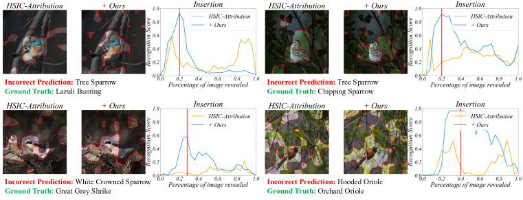
Figure 3: Visualization of the method for discovering what causes model prediction errors. The Insertion curve shows the correlation between the searched region and ground truth class prediction confidence. The highlighted region matches the searched region indicated by the red line in the curve, and the dark region is the error cause identified by the method.

5.4 Ablation Study

Components of Submodular Function

We analyze the impact of various submodular function-based score functions on the results for both the Celeb-A and CUB-200-2011 datasets, the saliency map generated by the HSIC-Attribution method is used as a prior. As shown in Table 3, we observed that using a single score function within the submodular function limits attribution faithfulness. When these score functions are combined in pairs, the faithfulness of our method will be further improved. We demonstrate that removing any of the four score functions leads to deteriorated Deletion and Insertion scores, confirming the validity of these score functions. We find that the effectiveness score is key for the Celeb-A dataset, while the collaboration score is more important for the CUB-200-2011 dataset.

Table 3: Ablation study on components of different score functions of submodular function on the Celeb-A, and CUB-200-2011 validation sets.

Submodular Function				Celeb-A		CUB-200-2011
Conf. Score	Eff. Score	Cons. Score	Colla. Score	Deletion ($\downarrow$)	Insertion ($\uparrow$)	Deletion ($\downarrow$)	Insertion ($\uparrow$)
(Equation 4)	(Equation 6)	(Equation 7)	(Equation 8)
✓	✗	✗	✗	0.3161	0.1795	0.3850	0.3455
✗	✓	✗	✗	0.1211	0.5615	0.0835	0.6383
✗	✗	✓	✗	0.2849	0.2291	0.1019	0.6905
✗	✗	✗	✓	0.1591	0.3053	0.0771	0.5409
✓	✓	✗	✗	0.1075	0.5714	0.0865	0.6624
✗	✓	✓	✗	0.1082	0.5692	0.0750	0.7111
✗	✗	✓	✓	0.1558	0.3617	0.0641	0.7181
✗	✓	✓	✓	0.1074	0.5735	0.0632	0.7169
✓	✗	✓	✓	0.1993	0.2616	0.0623	0.7227
✓	✓	✗	✓	0.1067	0.5712	0.0651	0.6753
✓	✓	✓	✗	0.1088	0.5750	0.0811	0.7090
✓	✓	✓	✓	0.1054	0.5752	0.0613	0.7262

Whether to Use a Priori Attribution Map

Our method uses existing attribution algorithms as priors when dividing the image into sub-regions. Table 4 shows the results, we directly divide the image into $N\times N$ patches without using a priori attribution map. Each element in the set only retains the pixel value of one patch area, and other areas are filled with values 0. We can observe that, whether on the Celeb-A dataset or the CUB-200-2011 dataset, the more patches are divided, the Deletion AUC score increases, and the fewer patches are divided, the Insertion AUC score increases. However, no matter how the number of patches is changed, we find that introducing a prior saliency map generated by the HSIC attribution method works best, in terms of Insertion or Deletion scores. Therefore, we believe that introducing a prior saliency map to assist in dividing image areas is effective and can improve the computational efficiency of the algorithm.

Table 4: Impact on whether to use a priori attribution map.

Method	Divided set size $m$	Celeb-A		CUB-200-2011
		Deletion ($\downarrow$)	Insertion ($\uparrow$)	Deletion ($\downarrow$)	Insertion ($\uparrow$)
Patch 7$\times$7	49	0.1493	0.5642	0.1061	0.6903
Patch 10$\times$10	100	0.1365	0.5459	0.1024	0.6159
Patch 14$\times$14	196	0.1284	0.5562	0.0853	0.5805
+HSIC-Attribution	25	0.1054	0.5752	0.0613	0.7262

6 Conclusion

In this paper, we propose a new method that reformulates the attribution problem as a submodular subset selection problem. To address the lack of attention to local regions, we construct a novel submodular function to discover more accurate fine-grained interpretation regions. Specifically, four different constraints implemented on sub-regions are formulated together to evaluate the significance of various subsets, i.e., confidence, effectiveness, consistency, and collaboration scores. The proposed method has outperformed state-of-the-art methods on two face datasets (Celeb-A and VGG-Face2) and a fine-grained dataset (CUB-200-2011). Experimental results show that the proposed method can improve the Deletion and Insertion scores for the correctly predicted samples. While for incorrectly predicted samples, our method excels in identifying the reasons behind the model’s decision-making errors.

Acknowledgments

This work was supported in part by the National Key R&D Program of China (Grant No. 2022ZD0118102), in part by the National Natural Science Foundation of China (No. 62372448, 62025604, 62306308), and part by Beijing Natural Science Foundation (No. L212004).

Appendix A Notations

The notations used throughout this article are summarized in Table 5.

Table 5: Some important notations used in this paper.

Notation	Description
$\mathbf{I}$	an input image
$\mathbf{I}^{M}$	a sub-region into which $\mathbf{I}$ is divided
$V$	a finite set of divided sub-regions
$S$	a subset of $V$
$\alpha$	an element from $V\setminus S$
$k$	the size of the $S$
$\mathcal{F}(\cdot)$	a function that maps a set to a value
$\mathcal{A}$	saliency map calculated by attribution algorithms
$N\times N$	the number of divided patches of $\mathbf{I}$
$m$	the number of sub-regions into which the image $\mathbf{I}$ is divided
$d$	the number of patches in $\mathbf{I}^{M}$
$\mathbf{x}$	an input sample
$\mathbf{y}$	the one-hot label
$u$	the predictive uncertainty ranges from 0 to 1
$F_{u}(\cdot)$	a deep evidential network for calculating the $u$ of $\mathbf{x}$
$F(\cdot)$	a traditional network encoder
$K$	the number of classes
$\mathrm{dist}(\cdot,\cdot)$	a function to calculate the distance between two feature vectors
$\bm{f}_{s}$	the target semantic feature vector

Appendix B Theory proof

B.1 Proof of Lemma 1

Proof.

Consider two sub-sets $S_{a}$ and $S_{b}$ in set $V$, where $S_{a}\subseteq S_{b}\subseteq V$. Given an element $\alpha$, where $\alpha=V\setminus S_{b}$. The necessary and sufficient conditions for the function $\mathcal{F}(\cdot)$ to satisfy the submodular property are:

$$\mathcal{F}\left(S_{a}\cup\{\alpha\}\right)-\mathcal{F}\left(S_{a}\right)\geq\mathcal{F}\left(S_{b}\cup\{\alpha\}\right)-\mathcal{F}\left(S_{b}\right).$$ (11)

For Eq. 4, assuming that the individual element $\alpha$ of the collection division is relatively small, according to the Taylor decomposition (Montavon et al., 2017), we can locally approximate $F_{u}(S_{a}+\alpha)=F_{u}(S_{a})+\nabla{F_{u}(S_{a})}\cdot\alpha$. Thus:

$$s_{\mathrm{conf.}}\left(S_{a}+\alpha\right)-s_{\mathrm{conf.}}\left(S_{a}\right) =\frac{K}{\exp\left(F_{u}\left(S_{a}\right)\right)+K}-\frac{K}{\exp\left(F_{u}\left(S_{a}+\alpha\right)\right)+K}$$ (12)

$$=\frac{K}{\exp\left(F_{u}\left(S_{a}\right)\right)+K}-\frac{K}{\exp\left(F_{u}\left(S_{a}\right)\right)\exp\left(\nabla{F_{u}(S_{a})}\cdot\alpha\right)+K},$$

since $S_{a}\cap\alpha=\varnothing$, $S_{a}$ and $\alpha$ do not overlap in the image space, and $\alpha$ is small. Therefore, we can regard $\nabla{F_{u}(S_{a})}\cdot\alpha\simeq 0$. Follow up:

$$s_{\mathrm{conf.}}\left(S_{a}+\alpha\right)-s_{\mathrm{conf.}}\left(S_{a}\right) \simeq\frac{K}{\exp\left(F_{u}\left(S_{a}\right)\right)+K}-\frac{K}{\exp\left(F_{u}\left(S_{a}\right)\right)\exp\left(\mathbf{0}\right)+K}$$ (13)

$$=0_{+},$$

and in the same way, $s_{\mathrm{conf.}}\left(S_{b}+\alpha\right)-s_{\mathrm{conf.}}\left(S_{b}\right)\simeq 0_{+}$. We have:

$$s_{\mathrm{conf.}}\left(S_{a}+\alpha\right)-s_{\mathrm{conf.}}\left(S_{a}\right)-\left(s_{\mathrm{conf.}}\left(S_{b}+\alpha\right)-s_{\mathrm{conf.}}\left(S_{b}\right)\right)\approx 0.$$ (14)

For Eq. 6, when a new element $\alpha$ is added to the set $S_{a}$, the minimum distance between elements in $S_{a}$ and other elements may be further reduced, i.e., for any element $s_{i}\in S_{a}$, we have $\min_{s_{j}\in S_{a}\cup\{\alpha\},s_{j}\neq s_{i}}{\mathrm{dist}\left(F\left(s_{i}\right),F\left(s_{j}\right)\right)}\leq\min_{s_{j}\in S_{a},s_{j}\neq s_{i}}{\mathrm{dist}\left(F\left(s_{i}\right),F\left(s_{j}\right)\right)}$. Thus:

$$s_{\mathrm{eff.}}\left(S_{a}\cup\{\alpha\}\right) =\min_{s_{i}\in S_{a}}{\mathrm{dist}\left(F\left(\alpha\right),F\left(s_{i}\right)\right)}+\sum_{s_{i}\in S_{a}}{\min_{s_{j}\in S_{a}\cup\{\alpha\},s_{j}\neq s_{i}}}{\mathrm{dist}\left(F\left(s_{i}\right),F\left(s_{j}\right)\right)}$$ (15)

$$=\min_{s_{i}\in S_{a}}{\mathrm{dist}\left(F\left(\alpha\right),F\left(s_{i}\right)\right)}+\sum_{s_{i}\in S_{a}}{\min_{s_{j}\in S_{a},s_{j}\neq s_{i}}}{\mathrm{dist}\left(F\left(s_{i}\right),F\left(s_{j}\right)\right)}-\varepsilon_{a},$$

where $\varepsilon_{a}$ is a constant, which is the sum of the minimum distance reductions of the elements in the original $S_{a}$ after $\alpha$ is added. Then, we have:

$$s_{\mathrm{eff.}}\left(S_{a}\cup\{\alpha\}\right)-s_{\mathrm{eff.}}\left(S_{a}\right)=\min_{s_{i}\in S_{a}}{\mathrm{dist}\left(F\left(\alpha\right),F\left(s_{i}\right)\right)}-\varepsilon_{a},$$ (16)

and in the same way,

$$s_{\mathrm{eff.}}\left(S_{b}\cup\{\alpha\}\right)-s_{\mathrm{eff.}}\left(S_{b}\right)=\min_{s_{i}\in S_{b}}{\mathrm{dist}\left(F\left(\alpha\right),F\left(s_{i}\right)\right)}-\varepsilon_{b},$$ (17)

since $S_{a}\subseteq S_{b}$, the minimum distance between alpha and elements in $S_{b}\setminus S_{a}$ may be smaller than the minimum distance between alpha and elements in $S_{a}$, thus,

$$\min_{s_{i}\in S_{a}}{\mathrm{dist}\left(F\left(\alpha\right),F\left(s_{i}\right)\right)}\geq\min_{s_{i}\in S_{b}}{\mathrm{dist}\left(F\left(\alpha\right),F\left(s_{i}\right)\right)},$$

since there are more elements in $S_{b}$ than in $S_{a}$, more elements in $S_{b}$ have the shortest distance from $\alpha$, that, $\varepsilon_{b}\geq\varepsilon_{a}$. Therefore, we have:

$$s_{\mathrm{eff.}}\left(S_{a}\cup\{\alpha\}\right)-s_{\mathrm{eff.}}\left(S_{a}\right)\geq s_{\mathrm{eff.}}\left(S_{b}\cup\{\alpha\}\right)-s_{\mathrm{eff.}}\left(S_{b}\right).$$ (18)

For Eq. 7, let $G\left(S_{a}\right)=F\left(S_{a}\right)\cdot\bm{f}_{s}$. Assuming that the individual element $\alpha$ of the collection division is relatively small, according to the Taylor decomposition, we can locally approximate $G\left(S_{a}+\alpha\right)=G\left(S_{a}\right)+\nabla{G\left(S_{a}\right)}\cdot\alpha$. Assuming that the searched $\alpha$ is valid, i.e., $\nabla{G\left(S_{a}\right)}>0$. Thus:

$$s_{\mathrm{cons.}}\left(S_{a}+\alpha,\bm{f}_{s}\right)-s_{\mathrm{cons.}}\left(S_{a},\bm{f}_{s}\right) =\frac{G(S_{a})+\nabla{G\left(S_{a}\right)}\cdot\alpha}{\|F(S_{a})+\nabla{F\left(S_{a}\right)}\cdot\alpha\|\|\bm{f}_{s}\|}-\frac{G(S_{a})}{\|F(S_{a})\|\|\bm{f}_{s}\|}$$ (19)

$$\simeq\frac{\nabla{G\left(S_{a}\right)}\cdot\alpha}{\|F(S_{a})\|\|\bm{f}_{s}\|},$$

since $S_{a}\cap\alpha=\varnothing$, $S_{a}$ and $\alpha$ do not overlap in the image space, and $\alpha$ is small, $\nabla{G\left(S_{a}\right)}\cdot\alpha$ is small. Then, we have:

$$s_{\mathrm{cons.}}\left(S_{a}+\alpha,\bm{f}_{s}\right)-s_{\mathrm{cons.}}\left(S_{a},\bm{f}_{s}\right)-\left(s_{\mathrm{cons.}}\left(S_{b}+\alpha,\bm{f}_{s}\right)-s_{\mathrm{cons.}}\left(S_{b},\bm{f}_{s}\right)\right)\approx 0.$$ (20)

For Eq. 8, let $G\left(\mathbf{I}-S_{a}\right)=F\left(\mathbf{I}-S_{a}\right)\cdot\bm{f}_{s}$. Assuming that the individual element $\alpha$ of the collection division is relatively small, according to the Taylor decomposition, we can locally approximate $G\left(\mathbf{I}-S_{a}-\alpha\right)=G\left(\mathbf{I}-S_{a}\right)-\nabla G\left(\mathbf{I}-S_{a}\right)\cdot\alpha$. Assuming that the searched alpha is valid, i.e., $\nabla{G\left(\mathbf{I}-S_{a}\right)}>0$. Thus:

$$s_{\mathrm{colla.}}\left(S_{a}+\alpha,\mathbf{I},\bm{f}_{s}\right)-s_{\mathrm{colla.}}\left(S_{a},\mathbf{I},\bm{f}_{s}\right) =\frac{G\left(\mathbf{I}-S_{a}\right)}{\|F\left(\mathbf{I}-S_{a}\right)\|\|\bm{f}_{s}\|}-\frac{G\left(\mathbf{I}-S_{a}\right)-\nabla G\left(\mathbf{I}-S_{a}\right)\cdot\alpha}{\|F\left(\mathbf{I}-S_{a}-\alpha\right)\|\|\bm{f}_{s}\|}$$ (21)

$$\simeq\frac{\nabla G\left(\mathbf{I}-S_{a}\right)\cdot\alpha}{\|F\left(\mathbf{I}-S_{a}\right)\|\|\bm{f}_{s}\|},$$

since $\alpha$ is small, $\nabla{G\left(\mathbf{I}-S_{a}\right)}\cdot\alpha$ is small. Then, we have:

$$s_{\mathrm{colla.}}\left(S_{a}+\alpha,\mathbf{I},\bm{f}_{s}\right)-s_{\mathrm{colla.}}\left(S_{a},\mathbf{I},\bm{f}_{s}\right)-\left(s_{\mathrm{colla.}}\left(S_{b}+\alpha,\mathbf{I},\bm{f}_{s}\right)-s_{\mathrm{colla.}}\left(S_{b},\mathbf{I},\bm{f}_{s}\right)\right)\approx 0.$$ (22)

Combining Eq. 14, 18, 20, and 22 we can get:

$$\mathcal{F}\left(S_{a}\cup\{\alpha\}\right)-\mathcal{F}\left(S_{a}\right)\geq\mathcal{F}\left(S_{b}\cup\{\alpha\}\right)-\mathcal{F}\left(S_{b}\right),$$ (23)

hence, we can prove that Eq. 9 is a submodular function. ∎

B.2 Proof of Lemma 2

Proof.

Consider a subset $S$, given an element $\alpha$, assuming that $\alpha$ is contributing to interpretation. The necessary and sufficient conditions for the function $\mathcal{F}(\cdot)$ to satisfy the property of monotonically non-decreasing is:

$$\mathcal{F}\left(S\cup\{\alpha\}\right)-\mathcal{F}\left(S\right)>0,$$ (24)

where, for Eq. 4:

$$s_{\mathrm{conf.}}\left(S+\alpha\right)-s_{\mathrm{conf.}}\left(S\right)=\frac{K}{\exp\left(F_{u}\left(S\right)\right)+K}-\frac{K}{\exp\left(F_{u}\left(S\right)\right)\exp\left(\nabla{F_{u}(S)}\cdot\alpha\right)+K},$$ (25)

since $\alpha$ is contributing to interpretation, $\nabla{F_{u}(S)}>0$, and $\exp\left(\nabla{F_{u}(S)}\cdot\alpha\right)>1$, thus:

$$s_{\mathrm{conf.}}\left(S+\alpha\right)-s_{\mathrm{conf.}}\left(S\right)>0.$$ (26)

For Eq. 6,

$$s_{\mathrm{eff.}}\left(S\cup\{\alpha\}\right)-s_{\mathrm{eff.}}\left(S\right)=\min_{s_{i}\in S}{\mathrm{dist}\left(F\left(\alpha\right),F\left(s_{i}\right)\right)}-\varepsilon,$$

since effective element $\alpha$ are selected as much as possible, the value $\varepsilon$ will be small,

$$s_{\mathrm{eff.}}\left(S\cup\{\alpha\}\right)-s_{\mathrm{eff.}}\left(S\right)\simeq\min_{s_{i}\in S}{\mathrm{dist}\left(F\left(\alpha\right),F\left(s_{i}\right)\right)}>0.$$ (27)

For Eq. 7, assuming that the searched $\alpha$ is valid,

$$s_{\mathrm{cons.}}\left(S+\alpha,\bm{f}_{s}\right)-s_{\mathrm{cons.}}\left(S,\bm{f}_{s}\right)\simeq\frac{\nabla{G\left(S\right)}\cdot\alpha}{\|F(S)\|\|\bm{f}_{s}\|}>0,$$ (28)

likewise, for Eq. 8,

$$s_{\mathrm{colla.}}\left(S+\alpha,\mathbf{I},\bm{f}_{s}\right)-s_{\mathrm{colla.}}\left(S,\mathbf{I},\bm{f}_{s}\right)\simeq\frac{\nabla G\left(\mathbf{I}-S\right)\cdot\alpha}{\|F\left(\mathbf{I}-S\right)\|\|\bm{f}_{s}\|}>0.$$ (29)

Combining Eq. 26, 27, 28, and 29 we can get:

$$\mathcal{F}\left(S\cup\{\alpha\}\right)-\mathcal{F}\left(S\right)>0,$$ (30)

hence, we can prove that Eq. 9 is monotonically non-decreasing.

∎

Appendix C Implementation Details

We primarily employed CNN-based architectures to explain our models. For the face datasets, we evaluated recognition models that were trained using the ResNet-101 (He et al., 2016) architecture and the ArcFace (Deng et al., 2019) loss function, with an input size of $112\times 112$ pixels. For the CUB-200-2011 dataset, we evaluated a recognition model trained on the ResNet-101 architecture with a cross-entropy loss function and an input size of $224\times 224$ pixels. It’s worth noting that all the uncertainty models denoted as $F_{u}(\cdot)$ in Sec. 4.2 were trained using the ResNet101 architecture. Given that the face recognition task primarily involves face verification, we use the target semantic feature $\bm{f}_{s}$ in functions $s_{\mathrm{cons.}}\left(S,\bm{f}_{s}\right)$ and $s_{\mathrm{colla.}}\left(S,\mathbf{I},\bm{f}_{s}\right)$ to adopt features computed from the original image using a pre-trained feature extractor. For the CUB-200-2011 dataset, we directly implement the fully connected layer of the classifier for a specified class. For the two face datasets, we set $N=28$ and $m=98$. For the CUB-200-2011 dataset, we set $N=10$ and $m=25$. We conduct our experiments using the Xplique  repository, which offers baseline methods and evaluation tools. To evaluate the Deletion and Insertion AUC scores, we set $k$ to be the same as the set size $m$ to evaluate the importance ranking of different sub-regions. These experiments were performed on an NVIDIA 3090 GPU.

Appendix D Different Network Backbone

We verified the effect of our method on more CNN network architectures, including VGGNet-19 (Simonyan & Zisserman, 2015), MobileNetV2 (Sandler et al., 2018), and EfficientNetV2-M (Tan & Le, 2021). We adopted the same settings as the original network, with an input size of $224\times 224$ for VGGNet-19, $224\times 224$ for MobileNetV2, and $384\times 384$ for EfficientNetV2-M. We conduct the experiment under the same setting as those employed for ResNet-101. When employing VGGNet-19, our method outperforms the SOTA method HSIC-Attribution, achieving a 70.2% increase in the average highest confidence and a 5.2% improvement in the Insertion AUC score. While utilizing MobileNetV2, our method outperforms the SOTA method HSIC-Attribution, achieving an 84.2% increase in the average highest confidence and a 17.6% improvement in the Insertion AUC score. Similarly, with EfficientNetV2-M, our method surpasses HSIC-Attribution, achieving a 23.4% increase in the average highest confidence and an 8.5% improvement in the Insertion AUC score. This indicates the versatility and effectiveness of our method across various backbones. Note that the 400 incorrectly predicted samples used by these networks in the experiment are not exactly the same, given the differences across the networks.

Table 6: Evaluation on discovering the cause of incorrect predictions for different network backbones.

		Average highest confidence ($\uparrow$)
Backbone	Method	(0-25%)	(0-50%)	(0-75%)	(0-100%)	Insertion ($\uparrow$)
	Grad-CAM++ (Chattopadhay et al., 2018)	0.1323	0.2130	0.2427	0.2925	0.1211
	Grad-CAM++ (w/ ours)	0.1595	0.2615	0.3521	0.4263	0.1304
	Score-CAM (Wang et al., 2020)	0.1349	0.2125	0.2583	0.3058	0.1057
	Score-CAM (w/ ours)	0.1649	0.2624	0.3452	0.4224	0.1186
	HSIC-Attribution (Novello et al., 2022)	0.1456	0.1743	0.1906	0.2483	0.1297
VGGNet-19 (Simonyan & Zisserman, 2015)	HSIC-Attribution (w/ ours)	0.1745	0.2716	0.3477	0.4226	0.1365
	Grad-CAM++ (Chattopadhay et al., 2018)	0.1988	0.2447	0.2544	0.2647	0.1094
	Grad-CAM++ (w/ ours)	0.2424	0.3575	0.3934	0.4193	0.1672
	Score-CAM (Wang et al., 2020)	0.1896	0.2323	0.2449	0.2510	0.1073
	Score-CAM (w/ ours)	0.2491	0.3395	0.3796	0.4082	0.1622
	HSIC-Attribution (Novello et al., 2022)	0.1709	0.2091	0.2250	0.2493	0.1446
ResNet-101 (He et al., 2016)	HSIC-Attribution (w/ ours)	0.2430	0.3519	0.3984	0.4513	0.1772
	Grad-CAM++ (Chattopadhay et al., 2018)	0.1584	0.2820	0.3223	0.3462	0.1284
	Grad-CAM++ (w/ ours)	0.1680	0.3565	0.4615	0.5076	0.1759
	Score-CAM (Wang et al., 2020)	0.1574	0.2456	0.2948	0.3141	0.1195
	Score-CAM (w/ ours)	0.1631	0.3403	0.4283	0.4893	0.1667
	HSIC-Attribution (Novello et al., 2022)	0.1648	0.2190	0.2415	0.2914	0.1635
MobileNetV2 (Sandler et al., 2018)	HSIC-Attribution (w/ ours)	0.2460	0.4142	0.4913	0.5367	0.1922
	Grad-CAM++ (Chattopadhay et al., 2018)	0.2338	0.2549	0.2598	0.2659	0.1605
	Grad-CAM++ (w/ ours)	0.2502	0.3038	0.3146	0.3214	0.1795
	Score-CAM (Wang et al., 2020)	0.2126	0.2327	0.2375	0.2403	0.1572
	Score-CAM (w/ ours)	0.2442	0.2900	0.3029	0.3115	0.1745
	HSIC-Attribution (Novello et al., 2022)	0.2418	0.2561	0.2615	0.2679	0.1611
EfficientNetV2-M (Tan & Le, 2021)	HSIC-Attribution (w/ ours)	0.2616	0.3117	0.3235	0.3306	0.1748

Appendix E Hyperparameter Sensitivity Analysis

We explored the effects of different score function weighting on the CUB-200-2011 dataset. As shown in Table 7, we find that only when increasing the weight of Eq. 7, the Insertion AUC score will be slightly improved, and other indicators have no obvious effect. If the weight is set too high, it may cause other score functions to fail, resulting in a significant decline in indicator performance. Therefore, we do not need to pay too much attention to how to weigh these score functions. The default weight is set to 1.

Table 7: Ablation study on the effects of different score functions on the CUB-200-2011 validation set.

Conf. Score	Eff. Score	Cons. Score	Colla. Score	Deletion ($\downarrow$)	Insertion ($\uparrow$)
(Equation 4)	(Equation 6)	(Equation 7)	(Equation 8)
1	1	1	1	0.0613	0.7262
20	1	1	1	0.1333	0.5979
50	1	1	1	0.2529	0.4681
100	1	1	1	0.3198	0.4059
1	20	1	1	0.0753	0.6725
1	50	1	1	0.0781	0.6614
1	100	1	1	0.0793	0.6537
1	1	20	1	0.0645	0.7276
1	1	50	1	0.0664	0.7276
1	1	100	1	0.0689	0.7221
1	1	1	20	0.0597	0.7174
1	1	1	50	0.0615	0.7001
1	1	1	100	0.0657	0.7010

Appendix F Ablation on More Details

Ablation on division sub-region number $N\times N$ and set size $m$

In this section, we explore the impact of the size of the divided sub-region number $N\times N$ and the size of the set $m$ on attribution performance. The experimental settings are set by default unless otherwise specified. We conducted experiments on the Celeb-A dataset and the CUB-200-2011 dataset. For the Celeb-A dataset, as shown in Table 8, we found that the more granular the division on the face dataset, the better the attribution results can be achieved, however, the attribution effect at the pixel level will be relatively poor. For the face dataset, a better choice is set $N=28$ and $m=98$. On the CUB-200-2011 dataset, as shown in Table 9, the attribution effect at the pixel level is still relatively poor. Since the positions of birds in the CUB-200-2011 dataset vary greatly and the background is complex, the images are not suitable for too fine-grained division. For the CUB-200-2011 dataset, a better choice is to set $N=10$ and $m=4$.

Table 8: Ablation study on division sub-region number $N\times N$ and set size $m$ on the Celeb-A validation set. The input image size is $112\times 112$, the base attribution method is HSIC-Attribution (Novello et al., 2022).

Division method	Number of divided areas for a element	Collection size	Deletion ($\downarrow$)	Insertion ($\uparrow$)
Patch 28$\times$28	8	98	0.1054	0.5752
Patch 14$\times$14	2	98	0.1158	0.5703
Patch 14$\times$14	4	49	0.1133	0.5757
Patch 10$\times$10	2	50	0.1288	0.5621
Patch 10$\times$10	4	25	0.1235	0.5645
Patch 8$\times$8	2	32	0.1276	0.5542
Pixel 112$\times$112	128	98	0.1258	0.5404
Pixel 112$\times$112	256	49	0.1148	0.5615
Pixel 112$\times$112	392	32	0.1136	0.5664

Table 9: Ablation study on division sub-region number $N\times N$ and set size $m$ on the CUB-200-2011 validation set. The input image size is $224\times 224$, and the base attribution method is HSIC-Attribution (Novello et al., 2022).

Division method	Number of divided areas for a element	Collection size	Deletion ($\downarrow$)	Insertion ($\uparrow$)
Patch 14$\times$14	2	98	0.0769	0.6343
Patch 14$\times$14	4	49	0.0652	0.6661
Patch 10$\times$10	2	50	0.0689	0.6917
Patch 10$\times$10	4	25	0.0613	0.7262
Patch 8$\times$8	2	32	0.0686	0.7079
Pixel 224$\times$224	256	49	0.0859	0.5818
Pixel 224$\times$224	392	32	0.0768	0.6398

Ablation of score function on the attribution of incorrectly predicted samples

Since the attribution of mispredicted samples requires specifying the correct category, we mainly discuss the impact of Eq. 7 and Eq. 8 on the attribution of mispredicted samples because these equations involve specifying categories. The network backbone we studied is ResNet-101, and 400 samples in the CUB-200-2011 test set that were misclassified by this network were used as research objects. As shown in Table 10, when any score function is removed, regardless of the imputation algorithm it is based on, the average highest confidence and Insertion AUC score will decrease, with Eq. 7 having the greatest impact.

Table 10: Ablation study on submodular function score components for incorrectly predicted samples in the CUB-200-2011 dataset.

Method	Cons. Score	Colla. Score	Average highest confidence ($\uparrow$)				Insertion ($\uparrow$)
	(Equation 7)	(Equation 8)	(0-25%)	(0-50%)	(0-75%)	(0-100%)
Grad-CAM++ (w/ ours)	✗	✓	0.0821	0.1547	0.1923	0.2303	0.1122
Grad-CAM++ (w/ ours)	✓	✗	0.1654	0.2888	0.3338	0.3611	0.1452
Grad-CAM++ (w/ ours)	✓	✓	0.2424	0.3575	0.3934	0.4193	0.1672
Score-CAM (w/ ours)	✗	✓	0.0742	0.1348	0.1835	0.2237	0.1072
Score-CAM (w/ ours)	✓	✗	0.1383	0.2547	0.3131	0.3402	0.1306
Score-CAM (w/ ours)	✓	✓	0.2491	0.3395	0.3796	0.4082	0.1622
HSIC-Attribution (w/ ours)	✗	✓	0.1054	0.1803	0.2177	0.2600	0.1288
HSIC-Attribution (w/ ours)	✓	✗	0.2394	0.3479	0.3940	0.4220	0.1645
HSIC-Attribution (w/ ours)	✓	✓	0.2430	0.3519	0.3984	0.4513	0.1772

Ablation of division sub-region number $N\times N$ of incorrect sample attribution

Without using a priori saliency map, we study the impact of different patch division numbers on the error sample attribution effect, where the number of patches $m=N\times N$. We explore the impact of six different division sizes on the results. As depicted in Table 11, our results indicate that dividing the image into more patches yields higher average highest confidence scores (0-100%). However, excessive division can introduce instability in the early search area (0-25%). In summary, without incorporating a priori saliency maps for division, opting for a 10x10 patch division followed by subset selection appears to be the optimal choice.

Table 11: Ablation study on the effect of sub-region division size $N\times N$ in incorrect sample attribution.

Method	Average highest confidence ($\uparrow$)				Insertion ($\uparrow$)
	(0-25%)	(0-50%)	(0-75%)	(0-100%)
HSIC-Attribution (Novello et al., 2022)	0.1709	0.2091	0.2250	0.2493	0.1446
Patch 5$\times$5	0.2597	0.3933	0.4389	0.4514	0.1708
Patch 6$\times$6	0.2372	0.4025	0.4555	0.4720	0.1538
Patch 7$\times$7	0.2430	0.4289	0.4819	0.4985	0.1621
Patch 8$\times$8	0.1903	0.4005	0.4740	0.5043	0.1584
Patch 10$\times$10	0.2020	0.4065	0.4908	0.5237	0.1519
Patch 12$\times$12	0.1667	0.3816	0.4987	0.5468	0.1247

Appendix G Effectiveness

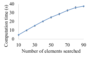
Figure 4: Processing time of our method.

In this section, we discuss the processing time effectiveness of the proposed algorithm. The size $m$ of the divided set we are testing is 98, we sequentially test the processing time required by our algorithm under different settings of the number of search elements $k$.

As shown in Fig. 4, the more elements are searched, the longer times it takes, and the relationship is almost linear. To use the proposed method efficiently, it is better to control the divided set size $m$, the size of the search set can be controlled by controlling the number of divided patches $N$, or by controlling the parameter $d$ that controls the number of patches assigned to each element.

Appendix H Visualizing Attribution of Correctly Predicted Classes

H.1 Celeb-A

The visualization results compared with the HSIC-Attribution method are shown in Fig. 5. Our method has a higher Insertion AUC curve area and searches for the highest confidence with higher attribution results than the HSIC-Attribution method.

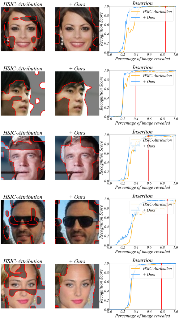
Figure 5: Visualization of the methods on the Celeb-A dataset.

H.2 CUB-200-2011

The visualization results compared with the HSIC-Attribution method are shown in Fig. 6. Our method has a higher Insertion AUC curve area and searches for the highest confidence with higher attribution results than the HSIC-Attribution method.

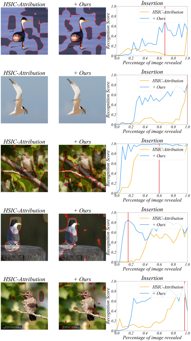
Figure 6: Visualization of the methods on the CUB-200-2011 dataset.

Appendix I Visualizing Attribution of Misclassified Prediction

Visualization of our method searches for causes of model prediction errors compared with the HSIC-Attribution method, as shown in Fig. 7. Our method has a higher Insertion AUC curve area and searches for the highest confidence with higher attribution results than the HSIC-Attribution method.

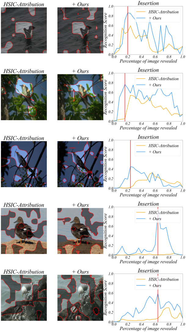
Figure 7: Visualization of the methods on CUB-200-2011 misclassified dataset.

Appendix J Limitation

The main limitation of our method is the computation time depending on the sub-region division approach. Specifically, we first divide the image into different subregions, and then we use the greed algorithm to search for the important subset regions. To accelerate the search process, we introduce the prior maps, which are computed based on the existing attribution methods. However, we observe that the performance of our attribution method is based on the scale of subregions, where the smaller regions would achieve much better accuracy as shown in the experiments. There exists a trade-off between the accuracy and the computation time. In the future, we will explore a better optimization strategy to solve this limitation.

References

- Arrieta et al. (2020) Alejandro Barredo Arrieta, Natalia Díaz-Rodríguez, Javier Del Ser, Adrien Bennetot, Siham Tabik, Alberto Barbado, Salvador García, Sergio Gil-López, Daniel Molina, Richard Benjamins, et al. Explainable Artificial Intelligence (XAI): Concepts, taxonomies, opportunities and challenges toward responsible AI. Information fusion, 58:82–115, 2020.
- Baehrens et al. (2010) David Baehrens, Timon Schroeter, Stefan Harmeling, Motoaki Kawanabe, Katja Hansen, and Klaus-Robert Müller. How to explain individual classification decisions. Journal of Machine Learning Research, 11:1803–1831, 2010.
- Bao et al. (2021) Wentao Bao, Qi Yu, and Yu Kong. Evidential deep learning for open set action recognition. In International Conference on Computer Vision (ICCV), pp. 13349–13358, 2021.
- Cao et al. (2018) Qiong Cao, Li Shen, Weidi Xie, Omkar M Parkhi, and Andrew Zisserman. VGGFace2: A dataset for recognising faces across pose and age. In IEEE International Conference on Automatic Face and Gesture Recognition (FG), pp. 67–74, 2018.
- Chattopadhay et al. (2018) Aditya Chattopadhay, Anirban Sarkar, Prantik Howlader, and Vineeth N Balasubramanian. Grad-CAM++: Generalized gradient-based visual explanations for deep convolutional networks. In Winter Conference on Applications of Computer Vision (WACV), pp. 839–847. IEEE, 2018.
- Chen et al. (2018) Jianbo Chen, Le Song, Martin Wainwright, and Michael Jordan. Learning to explain: An information-theoretic perspective on model interpretation. In International Conference on Machine Learning (ICML), pp. 883–892. PMLR, 2018.
- Chen et al. (2023) Ruoyu Chen, Jingzhi Li, Hua Zhang, Changchong Sheng, Li Liu, and Xiaochun Cao. Sim2Word: Explaining similarity with representative attribute words via counterfactual explanations. ACM Transactions on Multimedia Computing, Communications and Applications, 19(6):1–22, 2023.
- Deng et al. (2019) Jiankang Deng, Jia Guo, Niannan Xue, and Stefanos Zafeiriou. ArcFace: Additive angular margin loss for deep face recognition. In IEEE Conference on Computer Vision and Pattern Recognition (CVPR), pp. 4690–4699, 2019.
- Dwivedi et al. (2023) Rudresh Dwivedi, Devam Dave, Het Naik, Smiti Singhal, Rana Omer, Pankesh Patel, Bin Qian, Zhenyu Wen, Tejal Shah, Graham Morgan, et al. Explainable AI (XAI): Core ideas, techniques, and solutions. ACM Computing Surveys, 55(9):1–33, 2023.
- Edmonds (1970) Jack Edmonds. Submodular functions, matroids, and certain polyhedra. Combinatorial Structures and Their Applications, pp. 69–87, 1970.
- Elenberg et al. (2017) Ethan Elenberg, Alexandros G Dimakis, Moran Feldman, and Amin Karbasi. Streaming weak submodularity: Interpreting neural networks on the fly. In Annual Conference on Neural Information Processing Systems (NeurIPS), pp. 4044–4054, 2017.
- Fujishige (2005) Satoru Fujishige. Submodular functions and optimization. Elsevier, 2005.
- He et al. (2016) Kaiming He, Xiangyu Zhang, Shaoqing Ren, and Jian Sun. Deep residual learning for image recognition. In IEEE Conference on Computer Vision and Pattern Recognition (CVPR), pp. 770–778, 2016.
- Joseph et al. (2019) KJ Joseph, Krishnakant Singh, and Vineeth N Balasubramanian. Submodular batch selection for training deep neural networks. In International Joint Conference on Artificial Intelligence (IJCAI), pp. 2677–2683, 2019.
- Kothawade et al. (2022) Suraj Kothawade, Saikat Ghosh, Sumit Shekhar, Yu Xiang, and Rishabh Iyer. Talisman: targeted active learning for object detection with rare classes and slices using submodular mutual information. In European Conference on Computer Vision (ECCV), pp. 1–16. Springer, 2022.
- Li et al. (2021a) Jiahui Li, Kun Kuang, Lin Li, Long Chen, Songyang Zhang, Jian Shao, and Jun Xiao. Instance-wise or class-wise? a tale of neighbor shapley for concept-based explanation. In ACM International Conference on Multimedia (ACM MM), pp. 3664–3672, 2021a.
- Li et al. (2023) Jiapeng Li, Ping Wei, Wenjuan Han, and Lifeng Fan. IntentQA: Context-aware video intent reasoning. In International Conference on Computer Vision (ICCV), pp. 11963–11974, 2023.
- Li et al. (2021b) Jingzhi Li, Lutong Han, Ruoyu Chen, Hua Zhang, Bing Han, Lili Wang, and Xiaochun Cao. Identity-preserving face anonymization via adaptively facial attributes obfuscation. In ACM International Conference on Multimedia (ACM MM), pp. 3891–3899, 2021b.
- Liang et al. (2023a) Jiawei Liang, Siyuan Liang, Aishan Liu, Ke Ma, Jingzhi Li, and Xiaochun Cao. Exploring inconsistent knowledge distillation for object detection with data augmentation. In ACM International Conference on Multimedia (ACM MM), pp. 768–778, 2023a.
- Liang et al. (2024) Jiawei Liang, Siyuan Liang, Aishan Liu, Xiaojun Jia, Junhao Kuang, and Xiaochun Cao. Poisoned forgery face: Towards backdoor attacks on face forgery detection. arXiv preprint arXiv:2402.11473, 2024.
- Liang et al. (2022a) Siyuan Liang, Longkang Li, Yanbo Fan, Xiaojun Jia, Jingzhi Li, Baoyuan Wu, and Xiaochun Cao. A large-scale multiple-objective method for black-box attack against object detection. In European Conference on Computer Vision (ECCV), pp. 619–636, 2022a.
- Liang et al. (2022b) Siyuan Liang, Aishan Liu, Jiawei Liang, Longkang Li, Yang Bai, and Xiaochun Cao. Imitated detectors: Stealing knowledge of black-box object detectors. In ACM International Conference on Multimedia (ACM MM), pp. 4839–4847, 2022b.
- Liang et al. (2023b) Siyuan Liang, Mingli Zhu, Aishan Liu, Baoyuan Wu, Xiaochun Cao, and Ee-Chien Chang. BadCLIP: Dual-embedding guided backdoor attack on multimodal contrastive learning. arXiv preprint arXiv:2311.12075, 2023b.
- Liu et al. (2015) Ziwei Liu, Ping Luo, Xiaogang Wang, and Xiaoou Tang. Deep learning face attributes in the wild. In International Conference on Computer Vision (ICCV), pp. 3730–3738, 2015.
- Lundberg & Lee (2017) Scott M Lundberg and Su-In Lee. A unified approach to interpreting model predictions. In Annual Conference on Neural Information Processing Systems (NeurIPS), pp. 4765–4774, 2017.
- Mirzasoleiman et al. (2015) Baharan Mirzasoleiman, Ashwinkumar Badanidiyuru, Amin Karbasi, Jan Vondrák, and Andreas Krause. Lazier than lazy greedy. In AAAI Conference on Artificial Intelligence (AAAI), pp. 1812–1818, 2015.
- Montavon et al. (2017) Grégoire Montavon, Sebastian Lapuschkin, Alexander Binder, Wojciech Samek, and Klaus-Robert Müller. Explaining nonlinear classification decisions with deep taylor decomposition. Pattern recognition, 65:211–222, 2017.
- Nemhauser et al. (1978) George L Nemhauser, Laurence A Wolsey, and Marshall L Fisher. An analysis of approximations for maximizing submodular set functions—i. Mathematical programming, 14:265–294, 1978.
- Noroozi & Favaro (2016) Mehdi Noroozi and Paolo Favaro. Unsupervised learning of visual representations by solving jigsaw puzzles. In European Conference on Computer Vision (ECCV), pp. 69–84. Springer, 2016.
- Novello et al. (2022) Paul Novello, Thomas Fel, and David Vigouroux. Making sense of dependence: Efficient black-box explanations using dependence measure. In Annual Conference on Neural Information Processing Systems (NeurIPS), pp. 4344–4357, 2022.
- Pervez et al. (2023) Adeel Pervez, Phillip Lippe, and Efstratios Gavves. Scalable subset sampling with neural conditional poisson networks. In International Conference on Learning Representations (ICLR), pp. 1–21, 2023.
- Petsiuk et al. (2018) Vitali Petsiuk, Abir Das, and Kate Saenko. RISE: Randomized input sampling for explanation of black-box models. In British Machine Vision Conference (BMVC), pp. 151, 2018.
- Petsiuk et al. (2021) Vitali Petsiuk, Rajiv Jain, Varun Manjunatha, Vlad I Morariu, Ashutosh Mehra, Vicente Ordonez, and Kate Saenko. Black-box explanation of object detectors via saliency maps. In IEEE Conference on Computer Vision and Pattern Recognition (CVPR), pp. 11443–11452, 2021.
- Redmon & Farhadi (2018) Joseph Redmon and Ali Farhadi. YOLOv3: An incremental improvement. arXiv preprint arXiv:1804.02767, 2018.
- Ribeiro et al. (2016) Marco Tulio Ribeiro, Sameer Singh, and Carlos Guestrin. ”why should i trust you?” explaining the predictions of any classifier. In ACM Knowledge Discovery and Data Mining (SIGKDD), pp. 1135–1144, 2016.
- Sandler et al. (2018) Mark Sandler, Andrew Howard, Menglong Zhu, Andrey Zhmoginov, and Liang-Chieh Chen. MobileNetV2: Inverted residuals and linear bottlenecks. In IEEE Conference on Computer Vision and Pattern Recognition (CVPR), pp. 4510–4520, 2018.
- Selvaraju et al. (2020) Ramprasaath R Selvaraju, Michael Cogswell, Abhishek Das, Ramakrishna Vedantam, Devi Parikh, and Dhruv Batra. Grad-CAM: Visual explanations from deep networks via gradient-based localization. International Journal of Computer Vision, 128(2):336–359, 2020.
- Sensoy et al. (2018) Murat Sensoy, Lance Kaplan, and Melih Kandemir. Evidential deep learning to quantify classification uncertainty. In Annual Conference on Neural Information Processing Systems (NeurIPS), pp. 3183–3193, 2018.
- Simonyan et al. (2014) K Simonyan, A Vedaldi, and A Zisserman. Deep inside convolutional networks: visualising image classification models and saliency maps. In ICLR (Workshop Poster), 2014.
- Simonyan & Zisserman (2015) Karen Simonyan and Andrew Zisserman. Very deep convolutional networks for large-scale image recognition. In International Conference on Learning Representations (ICLR), 2015.
- Smilkov et al. (2017) Daniel Smilkov, Nikhil Thorat, Been Kim, Fernanda Viégas, and Martin Wattenberg. SmoothGrad: Removing noise by adding noise. arXiv preprint arXiv:1706.03825, 2017.
- Sundararajan et al. (2017) Mukund Sundararajan, Ankur Taly, and Qiqi Yan. Axiomatic attribution for deep networks. In International Conference on Machine Learning (ICML), pp. 3319–3328. PMLR, 2017.
- Tan & Le (2021) Mingxing Tan and Quoc Le. EfficientNetV2: Smaller models and faster training. In International Conference on Machine Learning (ICML), pp. 10096–10106. PMLR, 2021.
- Tu et al. (2023) Haoqin Tu, Chenhang Cui, Zijun Wang, Yiyang Zhou, Bingchen Zhao, Junlin Han, Wangchunshu Zhou, Huaxiu Yao, and Cihang Xie. How many unicorns are in this image? a safety evaluation benchmark for vision llms. arXiv preprint arXiv:2311.16101, 2023.
- Wang et al. (2018) Hao Wang, Yitong Wang, Zheng Zhou, Xing Ji, Dihong Gong, Jingchao Zhou, Zhifeng Li, and Wei Liu. CosFace: Large margin cosine loss for deep face recognition. In IEEE Conference on Computer Vision and Pattern Recognition (CVPR), pp. 5265–5274, 2018.
- Wang et al. (2020) Haofan Wang, Zifan Wang, Mengnan Du, Fan Yang, Zijian Zhang, Sirui Ding, Piotr Mardziel, and Xia Hu. Score-CAM: Score-weighted visual explanations for convolutional neural networks. In Proceedings of the IEEE/CVF conference on computer vision and pattern recognition workshops, pp. 24–25, 2020.
- Wei et al. (2014) Kai Wei, Yuzong Liu, Katrin Kirchhoff, and Jeff Bilmes. Unsupervised submodular subset selection for speech data. In IEEE International Conference on Acoustics, Speech and Signal Processing (ICASSP), pp. 4107–4111. IEEE, 2014.
- Wei et al. (2015) Kai Wei, Rishabh Iyer, and Jeff Bilmes. Submodularity in data subset selection and active learning. In International Conference on Machine Learning (ICML), pp. 1954–1963. PMLR, 2015.
- Welinder et al. (2010) P Welinder, S Branson, T Mita, C Wah, F Schroff, S Be-longie, and P Perona. Caltech-UCSD Birds 200. Technical Report CNS-TR-2010–001. Technical report, Technical Report CNS-TR-2010–001, California Institute of Technology, 2010. 1, 2010.
- Ya et al. (2024) Mengxi Ya, Yiming Li, Tao Dai, Bin Wang, Yong Jiang, and Shu-Tao Xia. Towards faithful xai evaluation via generalization-limited backdoor watermark. In International Conference on Learning Representations (ICLR), 2024.
- Yang et al. (2019) Jiancheng Yang, Qiang Zhang, Bingbing Ni, Linguo Li, Jinxian Liu, Mengdie Zhou, and Qi Tian. Modeling point clouds with self-attention and gumbel subset sampling. In IEEE Conference on Computer Vision and Pattern Recognition (CVPR), pp. 3323–3332, 2019.
- Zhao et al. (2023) Bingchen Zhao, Haoqin Tu, Chen Wei, Jieru Mei, and Cihang Xie. Tuning LayerNorm in Attention: Towards efficient multi-modal llm finetuning. arXiv preprint arXiv:2312.11420, 2023.
- Zhou et al. (2016) Bolei Zhou, Aditya Khosla, Agata Lapedriza, Aude Oliva, and Antonio Torralba. Learning deep features for discriminative localization. In IEEE Conference on Computer Vision and Pattern Recognition (CVPR), pp. 2921–2929, 2016.