Deinterleaving of Discrete Renewal Process Mixtures with Application to Electronic Support Measures

Abstract

In this paper, we propose a new deinterleaving method for mixtures of discrete renewal Markov chains. This method relies on the maximization of a penalized likelihood score. It exploits all available information about both the sequence of the different symbols and their arrival times. A theoretical analysis is carried out to prove that minimizing this score allows to recover the true partition of symbols in the large sample limit, under mild conditions on the component processes. This theoretical analysis is then validated by experiments on synthetic data. Finally, the method is applied to deinterleave pulse trains received from different emitters in a RESM (Radar Electronic Support Measurements) context and we show that the proposed method competes favorably with state-of-the-art methods on simulated warfare datasets.

Keywords: Deinterleaving, renewal process, maximum likelihood estimation, Electronic Support Measure, RADAR

1 Introduction

We consider the following problem. A sequence $z^{n}=z_{0},z_{1},\dots,z_{n-1}$ of $n$ symbols has been observed during a time window $\llbracket 0,T\rrbracket$, with $T\in\mathbb{N}$. The symbols $z_{i}$ of the sequence arrive at different integer time steps $t_{i}\in\mathbb{N}$, with $0\leq t_{0}\leq t_{1}\leq\dots\leq t_{n-1}\leq T$. $t^{n}$ is the sequence of arrival times of size $n$. Each symbol of $z^{n}$ is drawn from a finite set $\mathcal{A}$ (alphabet). The underlying generative model $P$ of this sequence is assumed to be a set of $E_{\Pi}>0$ Markov processes $G_{\Pi}(\{P^{e}\}_{e\in E(\Pi)})$, where $E(\Pi)$ is a set of emitters and $E_{\Pi}=|E(\Pi)|$ is the number of different emitters in this set. Each $P^{e}$, with $e\in E(\Pi)$, is an independent random process for emitter $e$, generating symbols in the sub-alphabet $A_{e}\subset\mathcal{A}$ with their corresponding arrival times. $\Pi=\{A_{e}\}_{e\in E(\Pi)}$ is the partition of $\mathcal{A}$ into the sub-alphabets $A_{e}$, which are assumed to be non-empty and disjoint. Given a sample $(z^{n},t^{n})$ from $P$, observed until time $T$, and without prior knowledge about the number of sub-alphabets $A_{e}$ (number of emitters), the deinterleaving problem of interest is to reconstruct the original partition $\Pi=\{A_{e}\}_{e\in E(\Pi)}$ of the alphabet.

This problem is motivated by an application in the context of electronic warfare, where an airborne ESM (Electronic Support Measure) receiver is located in an environment composed of many radars. This receiver intercepts pulse trains from multiple transmitters over a common channel. Each pulse is characterized by a frequency, which can be associated with a symbol $z_{i}$ in alphabet $\mathcal{A}$ (using a clustering method in frequency space), and a time of arrival (TOA), which can be discretized and assigned an integer value $t_{i}$. Other parameters such as pulse duration, power, or angle of arrival, may also be available, but in this work we restrict attention to the time and frequency information. In this context, the sub-alphabets $A_{e}$ correspond to the frequency channels used by the transmitters. They realize a partition of the total processed frequency band, which corresponds to the case where transmitters avoid mutual interference by controlling their access to the radio spectrum. The cases where different transmitters share common frequency channels is not addressed here. It corresponds to the case of non disjoint sub-alphabets which is out of the scope of this work. From the recorded pulse train, the aim of our problem is to determine how many radars are present in the environment and what signals are emitted by each radar.

The literature of deinterleaving RADAR signals is abundant. It was first performed in the literature by calculating histograms of received time differences [1, 2] or by estimating the phases of of the interleaved pulse trains [3]. This type of method has recently been revisited in [4], who proposed an agglomerative hierarchical clustering method combined with optimal transport distances. Such clustering methods deliver fast outcomes, but might fail in environments with complex radar patterns, potentially causing a performance degradation.

To overcome these limitations, another stream of work is based on inferring mixtures of Markov chains [5]. In these methods, a clustering algorithm is first applied to group the different pulses into different clusters, or letters, which correspond to the alphabet $\mathcal{A}$. Then, in a second step, these letters are partitioned into different sub-alphabets to identify the different emitters that could have generated the observed sequence of letters.

These methods are mainly based on two types of pulse train modeling in the literature: Interleaved Markov Process (IMP) and Mixture of Renewal Processes (MRP).

Modeling with IMP was introduced for the first time in [5]. This model does not directly take into account the arrival times of pulses, but rather considers their order of arrival. The overall interlaced sequence produced by the different transmitters and received in a single channel is modeled using a switching mechanism, whose role is to alternate the sequence of transmissions by the different emitters within the observed sequence. The inference of an IMP is generally carried out using non-parametric methods, by maximizing a global penalized likelihood score. When sub-alphabets are disjoint, i.e., each symbol can only be transmitted by a single transmitter, a deinterleaving scheme has been proposed in [6]. The authors proved the convergence of this method under mild conditions on switching and component processes, and provided that all possible partitions of letters can be evaluated. However, as the exploration of all possible partitions grows exponentially with the number of different symbols, the evaluation of all candidate partitions may be unfeasible in practice. Therefore, different search heuristics have recently been proposed to explore the partition space: an iterated local search in [7, 6], and a memetic algorithm in [8]. Meanwhile, [9] has proposed a variant of the IMP model introduced in [6] for the case of non-disjoint sub-alphabets inferred with an expectation maximization (EM) algorithm. The asymptotic consistency of this deinterleaving scheme is not proven.

These IMP models do not explicitly take into account the delay between the different signals in the deinterleaving scheme, but only their order of arrival. This feature makes them robust to disturbances that may occur during arrival time measurements, but does not take advantage of all available information. However, this information can be critical to the deinterleaving process because the times between different pulses generally follow regular, identifiable distributions.

Therefore, another category of methods has emerged in the literature based on inference of mixtures of Markov renewal processes. In these models, there is no switching mechanism, and the global generation model consists of a set of independent Markov renewal chains, or semi-Markov processes, which have been studied in detail in the discrete case, notably in [10]. Estimation of mixtures of semi-Markov chains has been carried out in [11] for continuous data or discrete data generated by a negative binomial distribution. The authors used an expectation maximization (EM) algorithm. Another method for deinterleaving a mixture of renewal processes has recently been proposed in [12]. This model is designed for continuous data and relies solely on temporal information. The proposed model assumes that the number of emitters is known in advance and that there are no labels on individual pulses.

In this paper, we aim to achieve the best of both worlds, namely to take into account all available information, such as pulse characteristics and arrival times, by modeling a mixture of renewal processes as in [11]. We also aim to propose a consistent deinterleaving scheme, as it has been done for IMP models [6], enabling the true partition to be recovered with probability tending towards one when sufficient data is provided. We would also like to take advantage of recent advances to explore the symbol partition space proposed by [8] and applied to the deinterlacing of RADAR pulse trains.

This paper is organized as follows. Section 2 presents the renewal processes mixture model. Section 3 describes the estimation of the parameters and the deinterleaving method to retrieve the partition of the symbols. Section 4 presents the experimental setting and a first experimental analysis of the consistency of the score. Section 5 reports on empirical results of the proposed method compared to the state of the art. Section 6 discusses the contribution and presents some perspectives for future work.

2 Mixture of renewal processes

The underlying generative model $P$ of the observed sequence $(z^{n},t^{n})$ is assumed to be a set of $E_{\Pi}>0$ independent Markov processes $G_{\Pi}(\{P^{e}\}_{e\in E(\Pi)})$.

2.1 Markov renewal chains

Given a sequence $z$ of symbols in the alphabet $\mathcal{A}$, for each process $P^{e}$ associated to the sub-alphabet $A_{e}$, we note $z[A_{e}]$ the sub-string of the sequence $z$ obtained by deleting all symbols not in $A_{e}$ and $t[A_{e}]$ the corresponding sequence of arrival times.

Each process $P^{e}$, with $e\in E(\Pi)$, is modeled as a Markov renewal chain $(Z^{e},T^{e})$ with:

• the chain $Z^{e}=(z^{e}_{l})_{l\in\mathbb{N}}=(z[A_{e}]_{l})_{l\in\mathbb{N}}$ with state space $A_{e}$, generating a sequence of symbols $z[A_{e}]$;

• the chain $T^{e}=(t^{e}_{l})_{l\in\mathbb{N}}$ generating the times of arrival of the symbols in $z^{e}_{l}$. We suppose that $t^{e}_{0}<t^{e}_{1}<\dots<t^{e}_{l}$, with $t^{e}_{0}=0$.

For each process $P^{e}$, we introduce also the chain $X^{e}=(x_{l}^{e})_{l\in\mathbb{N}^{*}}$, corresponding to the sojourn time in each state of the chain $Z^{e}$. For all $l\in\mathbb{N}^{*}$, $x_{l}^{e}=t^{e}_{l}-t^{e}_{l-1}>0$. By convention we set $x_{0}^{e}=0$.

For each letter $a$ in a sub-alphabet $A_{e}$, we assume that each sojourn time is drawn in a finite set $K^{a}$ of strictly positive integers. In the following, for a given emitter $e\in E(\Pi)$, we also note $K_{e}=\bigcup_{a\in A_{e}}K^{a}$ as the union of sojourn time sets of all symbols from $A_{e}$.

Each chain $(Z^{e},T^{e})$ satisfies for all $l\in\mathbb{N}$, for all $i,j\in A_{e}$, and for all $k\in K^{i}$

$$P^{e}(z^{e}_{l+1}=j,t^{e}_{l+1}-t^{e}_{l}=k|z^{e}_{0},\dots,z^{e}_{l};t^{e}_{0},\dots,t^{e}_{l})=P^{e}(z^{e}_{l+1}=j|z^{e}_{l}=i)\times P^{e}(t^{e}_{l+1}-t^{e}_{l}=k|z^{e}_{l}=i).$$ (1)

This equation means that, being in at a given state $i$ at time $t$, the next state $j$ is independent of the sojourn time in state $i$. We make this assumption in order to reduce the number of parameters to be estimated and therefore speed up the likelihood calculations, although in practice this is not always true, since some agile radar waveforms may consist of a periodically repeated synchronized time-frequency pattern. In some other cases, Equation (1) may hold at least approximately. We assume (and empirically confirm in our context) that the likelihood expression derived from Equation (1) is robust enough to produce good deinterleaving performance in practice.

Moreover, we assume that each process $P^{e}$ is time homogeneous. Therefore $P^{e}(z^{e}_{l+1}=j|z^{e}_{l}=i)$ and $P^{e}(t^{e}_{l+1}-t^{e}_{l}=k|z^{e}_{l}=i)$ are independent of $l$.

We denote by $\mathbf{P}^{e}=(p^{e}_{i,j})$ the transition matrix of $Z^{e}$, with for $i,j\in A_{e}$ $p^{e}_{i,j}=P^{e}(z^{e}_{l+1}=j|z^{e}_{l}=i),l\in\mathbb{N}$ and for $l\in\mathbb{N^{*}}$, $i\in A_{e}$, $k\in K^{i}$, we introduce the quantity $q^{e}_{i,k}=P^{e}(x_{l+1}=k|z^{e}_{l}=i)$.

Assumption $(\mathcal{P})$. For $i,j\in A_{e}$, we assume that $p^{e}_{i,j}>0$.
Assumption $(\mathcal{Q})$. For each $i\in A_{e},k\in K^{i}$, we assume that $q^{e}_{i,k}>0$.

According to this model, under assumptions $(\mathcal{P})$ and $(\mathcal{Q})$, it is possible to establish a first general uniqueness result for the underlying partition associated with the set of Markov processes that generated the observed data. The proof of Theorem 1 is given in the appendix.

Theorem 1.

Given a generative model $P=G_{\Pi}(\{P^{e}\}_{e\in E(\Pi)})$, corresponding to a partition $\Pi$ of the alphabet $\mathcal{A}$. Then, under assumptions $(\mathcal{P})$ and $(\mathcal{Q})$, if $P=G_{\Pi^{\prime}}(\{P^{e}\}_{e\in E(\Pi^{\prime})})$ for some partition $\Pi^{\prime}$, then $\Pi=\Pi^{\prime}$ must hold.

3 Deinterleaving Scheme

In this section, the estimation of the different components of the proposed discrete renewal process mixture is described and a consistent penalized maximum likelihood entropy score is derived.

3.1 Semi-Markov Chain Estimation

For each transmitter $e$, and given an observed sequence $(z^{n},t^{n})$, observed during the time window $\llbracket 0,T\rrbracket$, we define the following quantities:

• $N^{e}_{i}(T)$, the number of symbols $i$ in the observed sequence $z^{n}[A_{e}]$ until time $T$.

• $N^{e}_{i,j}(T)$, the number of transitions from $i$ to $j$, observed in the sequence $z^{n}[A_{e}]$ until time $T$.

• $N^{e}_{i,k}(T)$, the number of transitions observed from $i$ to any other letter in $z^{n}[A_{e}]$ until time $T$, with sojourn time equal to $k$.

• $N^{e}(T)$, the total number of transitions observed in the sub-sequence $z^{n}[A_{e}]$ until time $T$.

For a transmitter $e$, which generates a sequence $z^{n}[A_{e}]$ with corresponding sequence of arrival times $t^{n}[A_{e}]$ observed during the time window $\llbracket 0,T\rrbracket$, according to Equation (1), the likelihood of $(z^{n}[A_{e}],t^{n}[A_{e}])$ is given by

$$\mathcal{L}^{T}_{A_{e}}(z^{n}[A_{e}],t^{n}[A_{e}])=P^{e}(z_{0})\prod_{l=0}^{N^{e}(T)-1}P^{e}(z^{e}_{l+1}|z^{e}_{l})P^{e}(t^{e}_{l+1}-t^{e}_{l}|z^{e}_{l})\overline{H}_{z_{N^{e}(T)}}(u_{T}),$$ (2)

with $\overline{H}_{i}(.)$ the survival function of sojourn time in state $i$, defined for $k\in\mathbb{N}$ by $\overline{H}_{i}(k)=P(x_{1}>k|z_{0}=i)$ and $u_{T}=T-t_{N^{e}(T)}$.

The approached likelihood is defined as

$$\bar{\mathcal{L}}^{T}_{A_{e}}(z^{n}[A_{e}],t^{n}[A_{e}])=\prod_{l=0}^{N^{e}(T)-1}P^{e}(z^{e}_{l+1}|z^{e}_{l})P^{e}(t^{e}_{l+1}-t^{e}_{l}|z^{e}_{l}).$$ (3)

Proposition 1.

The exact log-likelihood function $\text{log}(\mathcal{L}^{T}_{A_{e}}(z^{n}[A_{e}],t^{n}[A_{e}]))$ and the approached likelihood $\text{log}(\bar{\mathcal{L}}^{T}_{A_{e}}(z^{n}[A_{e}],t^{n}[A_{e}]))$ functions are asymptotically equivalent when $T\rightarrow\infty$.

As the exact log-likelihood function and the approached log-likelihood function are asymptotically equivalent, we will focus on the maximization of the approached log-likelihood.

Given the observed sub-sequence $z^{n}[A_{e}]$ with corresponding sequence of arrival times $t^{n}[A_{e}]$ observed until time $T$, for each transmitter $e$, we define the empirical estimators of the coefficients $p^{e}_{i,j}$ of the transition matrix $\mathbf{P}^{e}$ and the empirical estimators of the coefficients $q^{e}_{i_{k}}$ of the distributions of the sojourn times, respectively by $\hat{p}^{e}_{i,j}(T):=\frac{N^{e}_{i,j}(T)}{N^{e}_{i}(T)}$ and $\hat{q}^{e}_{i,k}(T):=\frac{N^{e}_{i,k}(T)}{N^{e}_{i}(T)}$.

Proposition 2.

The estimators $\hat{p}^{e}_{i,j}(T)$ and $\hat{q}^{e}_{i,k}(T)$ maximize the approached log-likelihood function $\text{log}(\bar{\mathcal{L}}^{T}_{A_{e}}(z^{n}[A_{e}],t^{n}[A_{e}]))$.

When using the estimators $\hat{p}^{e}_{i,j}(T)$ and $\hat{q}^{e}_{i,k}(T)$, the approached maximum likelihood of the sequence $(z^{n}[A_{e}],t^{n}[A_{e}])$ is denoted $\hat{\mathcal{L}}^{T}_{A_{e}}(z^{n}[A_{e}],t^{n}[A_{e}])$.

Given an observed sequence $(z^{n}[A_{e}],t^{n}[A_{e}])$, generated by transmitter $e$ and observed until time $T$, we denote $H^{T}_{A_{e}}(z^{n}[A_{e}],t^{n}[A_{e}])=-\text{log}(\hat{\mathcal{L}}^{T}_{A_{e}}(z^{n}[A_{e}],t^{n}[A_{e}]))$, the approached maximum likelihood entropy for transmitter $e$.

We have

$$H^{T}_{A_{e}}(z^{n}[A_{e}],t^{n}[A_{e}])=H^{T}_{Z,A_{e}}(z^{n}[A_{e}],t^{n}[A_{e}])+H^{T}_{X,A_{e}}(z^{n}[A_{e}],t^{n}[A_{e}]),$$ (4)

with $H^{T}_{Z,A_{e}}(z^{n}[A_{e}],t^{n}[A_{e}])$ the entropy of the transition process for transmitter $e$,

$$H^{T}_{Z,A_{e}}(z^{n}[A_{e}],t^{n}[A_{e}])=-\sum_{i,j\in A_{e}}N^{e}_{i,j}(T)\text{log}\ \frac{N^{e}_{i,j}(T)}{N^{e}_{i}(T)},$$ (5)

and $H^{T}_{X,A_{e}}(z^{n}[A_{e}],t^{n}[A_{e}])$ the entropy of the distribution of sojourn time for transmitter $e$:

$$H^{T}_{X,A_{e}}(z^{n}[A_{e}],t^{n}[A_{e}])=-\sum_{i\in A_{e}}\sum_{k\in K_{i}}N^{e}_{i,k}(T)\ \text{log}\ \frac{N^{e}_{i,k}(T)}{N^{e}_{i}(T)}.$$ (6)

3.2 Global model estimation and deinterleaving scheme

As all transmitters are independent, the global approached likelihood of the sequence $(z^{n},t^{n})$ observed until time $T$ and related to the partition $\Pi$ of the symbols is given by

$$\mathcal{L}^{T}_{\Pi}(z^{n},t^{n})=\prod_{e\in E(\Pi)}\mathcal{L}^{T}_{A^{e}}(z^{n}[A_{e}],t^{n}[A_{e}]).$$ (7)

We use $H^{T}_{\Pi}(z^{n},t^{n})=-\text{log}\ \hat{\mathcal{L}}^{T}_{\Pi}(z^{n},t^{n})$ to denote the corresponding approached maximum likelihood entropy. Thus, we have,

$$H^{T}_{\Pi}(z^{n},t^{n})=\sum_{e\in E(\Pi)}H^{T}_{A_{e}}(z^{n}[A_{e}],t^{n}[A_{e}]),$$ (8)

with $H^{T}_{A_{e}}(z^{n}[A_{e}],t^{n}[A_{e}])$ given by Equation (4).

Given a sequence $(z^{n},t^{n})$ observed until time $T$, the proposed deinterleaving scheme corresponds to finding $\hat{\Pi}$ minimizing a penalized maximum likelihood score function of the form

$$C^{T}_{\Pi}(z^{n},t^{n})=H^{T}_{\Pi}(z^{n},t^{n})+\beta E_{\Pi}\text{log}(n),$$ (9)

with $\beta$ a non-negative (penalization) constant and $E_{\Pi}$ the number of transmitters.

Assumption $(\mathcal{K})$. Let $K_{e}=\bigcup_{z\in A_{e}}K^{z}$ be the set of all sojourn times for transmitter $e$. For all transmitter $e\in E(\Pi)$, the greatest common divisor (gcd) of the set $K_{e}$ is equal to 1.

Under this additional assumption, we show with the following theorem that the deinterleaving scheme allows to retrieve the true partition when $T$ goes toward infinity, with an exhaustive search in the space of all possible partitions of the alphabet $\mathcal{A}$. This proof is reported in the appendix.

Theorem 2.

Let $P_{\Pi}=G_{\Pi}(\{P^{e}\}_{e\in E(\Pi)})$ and let $\Pi^{{}^{\prime}}$ be a partition of $\mathcal{A}$ such that $\Pi^{{}^{\prime}}\neq\Pi$. Then, under assumptions $(\mathcal{Q})$, $(\mathcal{K})$ and $(\mathcal{P})$, for any sample $(z^{n},t^{n})$ from $P_{\Pi}$ observed until time $T$, we have

$$\frac{1}{T}(C^{T}_{\Pi^{\prime}}(z^{n},t^{n})-C^{T}_{\Pi}(z^{n},t^{n}))\geq\Delta>0\ a.s\ as\ T\rightarrow\infty.$$ (10)

This is also true for any sample $(z^{n},t^{n})$ from $P_{\Pi}$ such that $P_{\Pi^{\prime}}((z^{n},t^{n}))>0$.

The second part of the theorem is very useful as it shows that the result not only holds due to the incompatibility of partitions. Even if, for instance, no simultaneous emission of different symbols occurs in the observed sequence (which can be rather unlikely for some scattered sets of emission delays), our deinterleaving process is able to identify the true partition if the observed sequence is sufficiently long.

Note that this results is valid for all non-negative values of the penalization constant $\beta$ entering in equation (9), and in particular when $\beta=0$, as it will be experimentally confirmed in Section 4 when using synthetic data generated according to the model described in Section 2.

However, we experimentally observe in practice, as shown in Section 5, that using $\beta>0$ can improve the results when applying the deinterleaving scheme in the ESM domain, whose incoming data does not exactly match the proposed model.

3.3 Solving the Combinatorial Problem in the Space of Partitions

Given an alphabet $\mathcal{A}$ and a sample $(z^{n},t^{n})$ observed until time $T$, finding the partition $\Pi$ minimizing the score $C^{T}_{\Pi}$ requires to solve a combinatorial problem in the search space of the alphabet partitions given by

$$\Omega_{\mathcal{A}}=\{\Pi|\mathcal{A}=\bigcup_{e\in E(\Pi)}A_{e}\wedge\forall(e,e^{\prime})\in E(\Pi)^{2},e\neq e^{\prime}\implies A_{e}\cap A_{e^{\prime}}=\emptyset\}.$$ (11)

The size of this search space can be calculated exactly with the Bell number:

$$B_{|\mathcal{A}|}=\sum_{k=0}^{|\mathcal{A}|}\frac{1}{k!}\sum_{i=0}^{k}(-1)^{i}\binom{k}{i}(k-i)^{|\mathcal{A}|}.$$ (12)

For a small number of letters (less than 10), as the size of $\Omega_{\mathcal{A}}$ remains reasonable (less than 115975), we can use an exhaustive search in the space of all partitions. This can be done efficiently using the algorithm proposed in [13].

However, since this space search grows exponentially with the number of letters, an exhaustive search is in general not feasible in a reasonable amount of time.

Therefore, when the number of letters is greater than 10, we propose to use an heuristic to find the best partition $\Pi$ in the huge search space $\Omega_{\mathcal{A}}$. We adapted the recent memetic algorithm MAAP, which was already used for a deinterleaving problem in [8], seen as a particular grouping problem. The MAAP algorithm uses a population of different candidate solutions (partitions). It alternates between two phases during the search. In the first phase, a local search procedure (tabu search) is performed to improve the partitions in the population. In the second phase, crossovers are performed between partitions to generate new candidate partitions, which are further improved by tabu search. The algorithm is efficiently implemented with incremental evaluation techniques, taking advantage of the fact that the likelihood score of each sub-alphabet $A_{i}$ can be calculated independently.

4 First experimental analysis

The first experiment studies the ability of the deinterleving scheme to retrieve the true partition, when the data are generated according to the ideal framework described in Section 2, with a collection of independent renewal processes, and when it is possible to perform an exhaustive search in the space $\Omega_{\mathcal{A}}$ of the partitions. We first describe the data generating process used for these experiments. Then we present an experimental analysis of the consistency of the score.

4.1 Synthetic dataset generation

The datasets are based on synthetic sequences $(z^{n},t^{n})$ of size $n$ generated by a set of $E_{\Pi}$ renewal processes $G_{\Pi}(\{P^{e}\}_{e\in E(\Pi)})$. Given a length $n$ and an alphabet $\mathcal{A}$, a scenario, i.e a sequence $(z^{n},t^{n})$, is generated as follow:

• From an alphabet $\mathcal{A}$, a ground truth partition $\Pi_{truth}=\{A_{e}\}_{e\in E(\Pi_{truth})}$ of the alphabet $\mathcal{A}$ is randomly and uniformly drawn in the search space $\Omega_{\mathcal{A}}$. $E_{\Pi}$ is the number of transmitters associated with this partition.

• For each transmitter ${e\in E(\Pi_{truth})}$, with corresponding sub-alphabet $A_{e}$, a probabilistic transition matrix $\mathbf{P}^{e}=(p^{e}_{i,j})$ of size $|A_{e}|\times|A_{e}|$ is randomly drawn with non-zero coefficients in order to satisfy assumption $(\mathcal{P})$.

• For each symbol $a$ in $\mathcal{A}$, a number of sojourn time states is randomly drawn in $\llbracket 1,K\rrbracket$, then different sojourn times $k_{a}$ are randomly drawn in the interval $\llbracket 1,L\rrbracket$, such that assumption $(\mathcal{K})$ is verified. $K$ and $L$ are two hyper-parameters of the generator, set up to the values $E_{\Pi_{truth}}+1$ and $|\mathcal{A}|+1$ respectively. Then, for each symbol $a$ in $\mathcal{A}$, a probability $q_{a,k_{a}}$ of each sojourn time $k^{a}$, is uniformly drawn such as $\sum_{k^{a}\in K^{a}}q_{a,k_{a}}=1$, and $\forall k^{a}\in K^{a},q_{a,k_{a}}>0$, in order to meet assumption $(\mathcal{Q})$.

• An initial state symbol $z^{e}_{0}$ of each process $P^{e}$ is randomly drawn in $A_{e}$.

• For each transmitter $P^{e}$ a sequence $(z^{e}_{l},t^{e}_{l})_{l\in\mathbb{N}}$ is generated using the initial state $z^{e}_{0}$, the transition matrix $\mathbf{P}^{e}$ and the distribution of sojourn times for each symbol $a\in A_{e}$.

• The $E_{\Pi_{truth}}$ sequences $(z^{e}_{l},t^{e}_{l})$ are merged to build a sequence $(z^{n},t^{n})$ of size $n$, with increasing times of arrival $0\leq t_{0}\leq t_{1}\leq\dots\leq t_{n-1}\leq T$.

Using this synthetic dataset generator, denoted as $G(\mathcal{A},n)$, we first study different scenarios with different sizes $n$ and a low number of symbols. This allows us to experimentally verify that the ground truth partition $\Pi_{truth}$ can be retrieved with probability one, when $n$ goes toward infinity and when an exhaustive search in the space of all partitions is performed.

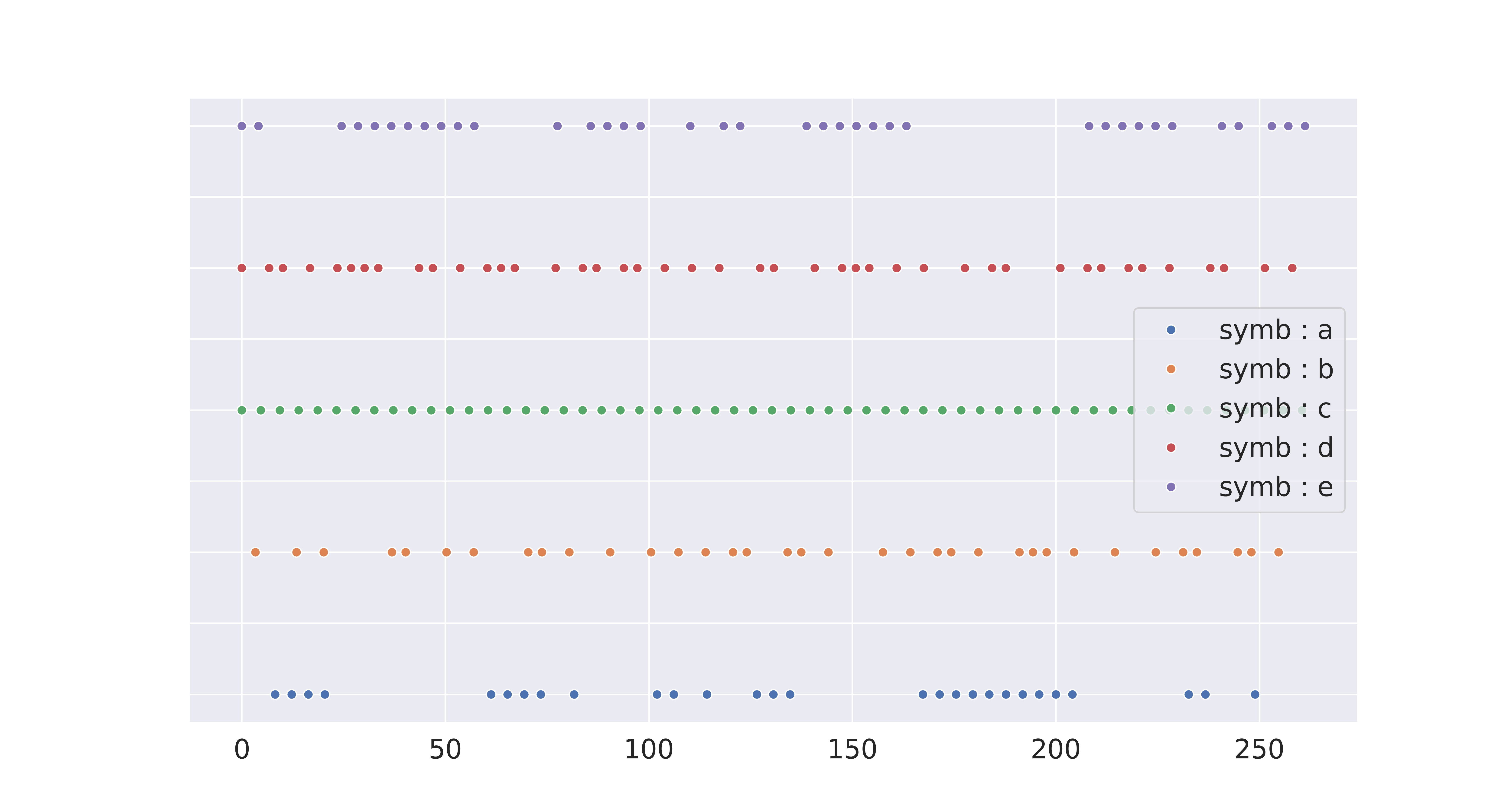
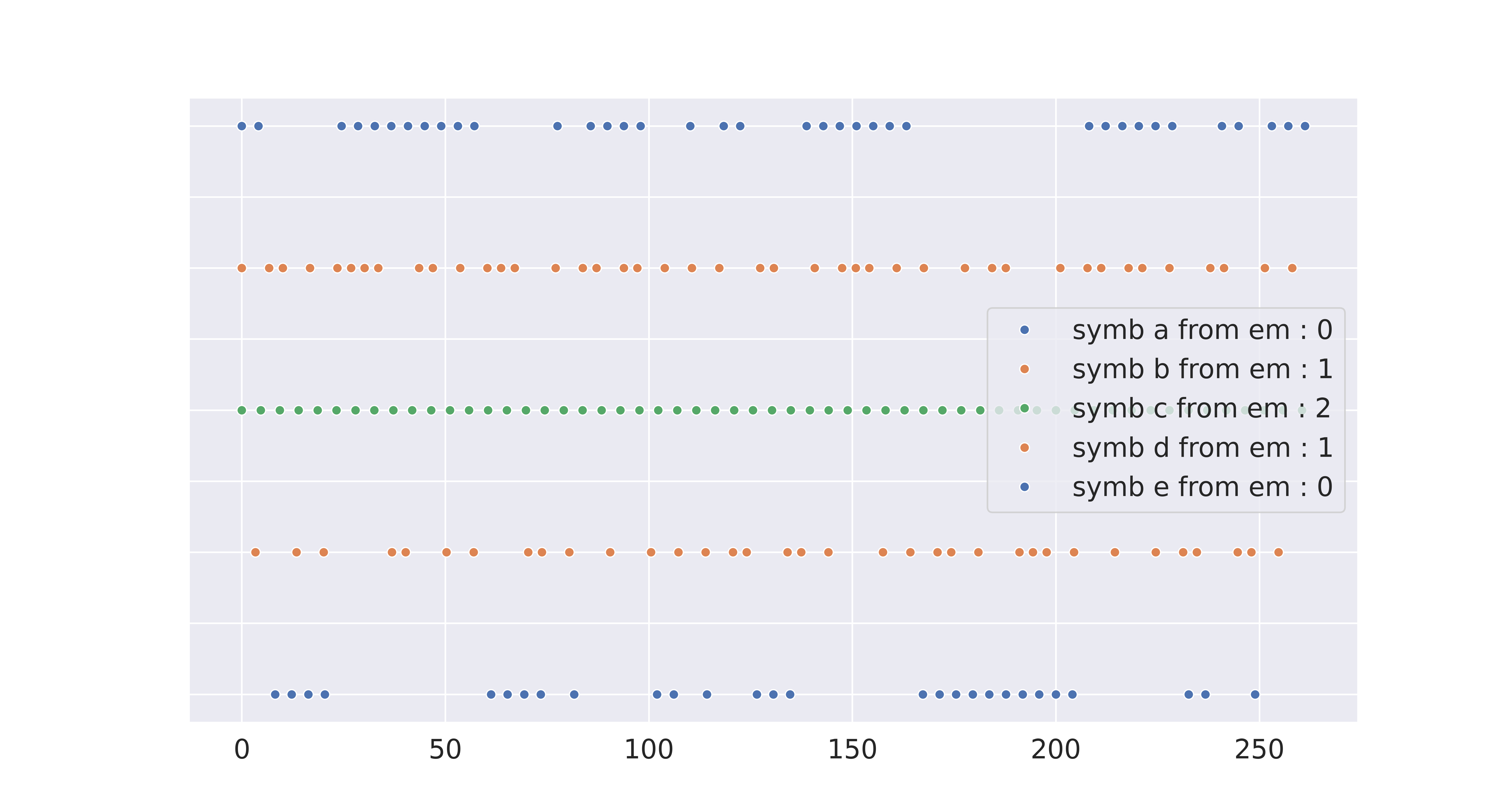
Figure 1: Display of data generated for a scenario of size 200, with 5 different symbols coming from 3 different emitters. The top graph shows the different symbols according to their arrival time. The second graph represents the ground truth, associating the corresponding symbol with each emitter.

Figure 1 illustrates an example of generated scenario with $|\mathcal{A}|=5$ and $n=200$. As displayed on the second plot, for this example, the ground truth is $\Pi_{truth}=\{a,e\}\cup\{b,d\}\cup\{c\}$, and there are 3 different transmitters indicated with blue, green and orange colors.

4.2 Empirical verification of the consistency of the score

In order to analyse the robustness of our deinterleaving scheme, we study different configurations with a number of symbols $|\mathcal{A}|\in\{3,5,7,9\}$ and a length $n$ ranging in the interval $\llbracket 0,5000\rrbracket$. For each configuration $(|\mathcal{A}|,n)$, 1000 different datasets $(\mathcal{A},\Pi_{truth},z^{n},t^{n})$ are independently generated.

For each of these datasets, an exhaustive search of the partition $\hat{\Pi}$ minimizing the score $C^{T}_{\hat{\Pi}}(z^{n},t^{n})$, given by Equation (9) and computed with $\beta=0$, is performed. At the end of this process, if $\hat{\Pi}$ is equal to $\Pi_{truth}$ (up to a permutation of the different sub-alphabets), we consider it a success, otherwise we consider it a failure.

Figure 2 shows the average success rate of this procedure computed for 1000 independent scenarios for each configuration $(|\mathcal{A}|,n)$.

These results confirm the convergence of the model even without penalization on the score (when $\beta=0$), as stated by Theorem 2. Indeed, we observe on this figure that for all scenarios with different numbers of symbols, that the success rate converges toward $100\%$ when the sequence length $n$ of the observed data $(z^{n},t^{n})$ increases.

We also observe a decrease in convergence speed with alphabet size. For alphabet sizes of $3,5,7,9$, the success rate reaches $99\%$ for sequence lengths $n$ equal to $460,875,1920,2395$ respectively. This can be explained by the greater number of parameters to be estimated as the alphabet size increases.

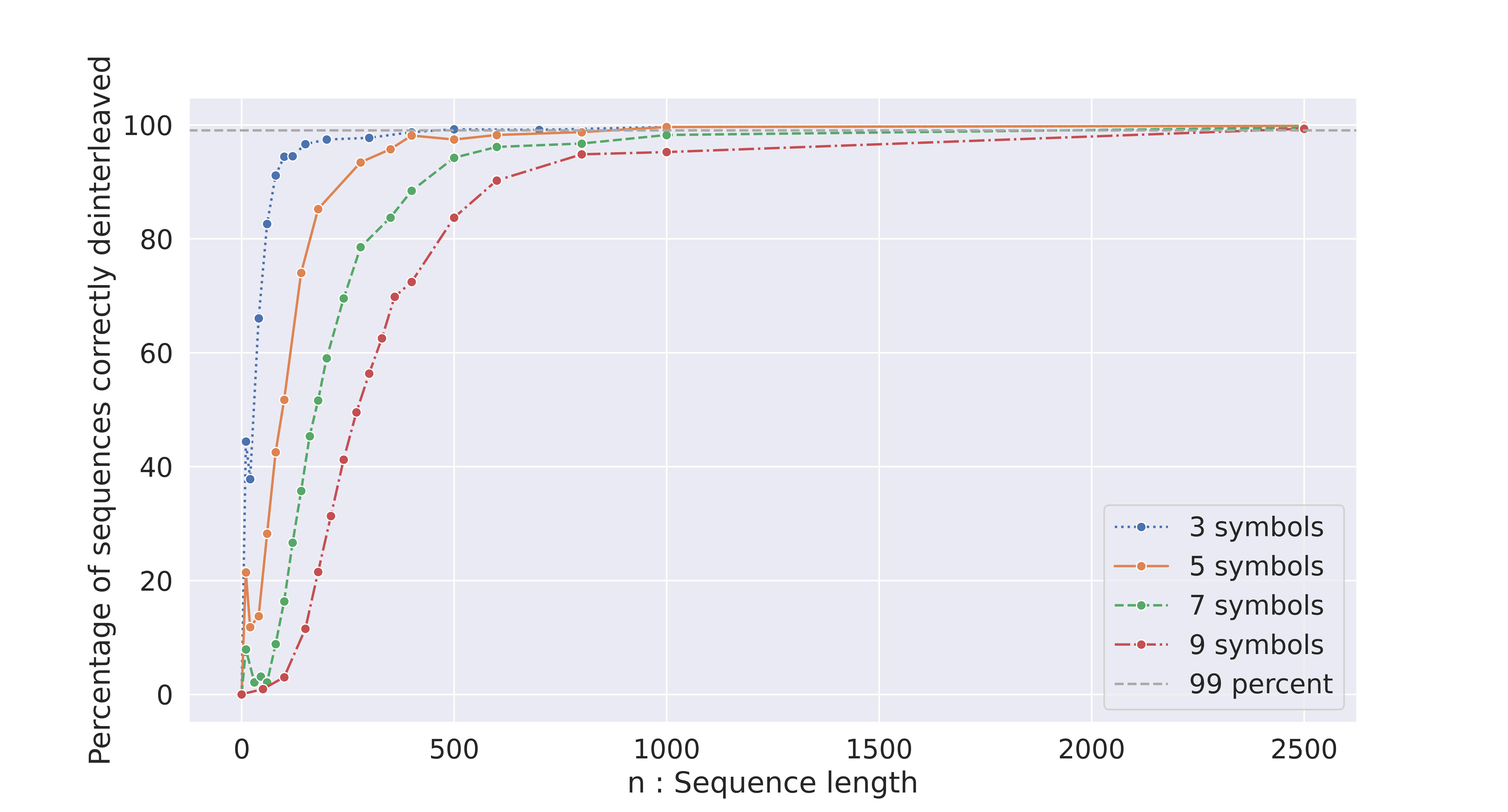
Figure 2: Average success rate of the proposed deinterleaving scheme when an exhaustive search in the partition space is performed and displayed for different numbers of symbols and different sequence sizes $n$. The horizontal line represents the $99\%$ threshold of correctly deinterlaced sequences.

5 Experimental validation on deinterleaving benchmarks

The goal of this section is to evaluate the performance of the proposed algorithm called TEDS for Temporal Estimation Deinterleaving Scheme in comparison with state-of-the-art algorithms of the literature. The TEDS algorithm corresponds to the evaluation of the score presented in Section 3.2 coupled with the memetic algorithm mentioned in Section 3.3 for the exploration of the partition space.

This section first describes the baseline algorithms, followed by their hyper-parameter settings used in the experiments.

Subsection 5.3 reports the experimental results obtained on the synthetic datasets with 5, 10, 20 and 50 symbols coming from the generator presented in the last section. Then, in subsection 5.4 we present results on datasets coming from an ESM data generator, which simulates realistic situations with mobile radar warning receivers.

5.1 State-of-the-art algorithms

For comparison with the state of the art, the following algorithms have been re-implemented in Python 3 from the authors’ original papers:

• The improved SDIF algorithm from [14]. SDIF is an algorithm first proposed in [2], which is a well-known reference in the RADAR community. It aims to identify different letter sub-sequences based on the calculation of histograms of observed sojourn times.

• OT: the deinterlacing algorithm proposed in [4]. In this algorithm, a matrix of optimal transport distance is first computed between all sub-sequences of symbols. Then, according to this distance matrix, a hierarchical clustering method is applied to group the different sequences.

• IMP: the deinterleaving scheme proposed in [6] with the exploration of the partition space developed by [7]. In this approach, the underlying generative model of the sequence is assumed to be an interleaved Markov process $P=\mathcal{I}_{\Pi}(P_{1},\dots,P_{m};P_{w})$, where $m>0$ is the unknown number of different transmitters, $P_{i}$ is an independent component random process for transmitter $i$, generating symbols in the sub-alphabet $A_{i}\subset\mathcal{A}$, $P_{w}$ is a random switch process over transmitters. The vector $\textbf{k}=(k_{1},\dots,k_{m};k_{w})$ corresponds to the different orders of the components and switch Markov processes. The authors proposed a deinterleaving scheme, given by minimizing a global cost function:

  $$(\hat{\Pi},\hat{\textbf{k}})=\underset{(\Pi,\textbf{k})}{argmin}\ C_{(\Pi,\textbf{k})}(z^{n}),$$ (13)

  with $C_{(\Pi,\textbf{k})}(z^{n})$ a global penalized maximum likelihood (ML) entropy score of the sequence $z^{n}$ (sorted by increasing times of arrival $t^{n}$) under the IMP model defined as

  $$C_{(\Pi,\textbf{k})}(z^{n})=\sum_{i=1}^{m}\hat{H}_{k_{i}}(z^{n}[A_{i}])+\hat{H}_{k_{w}}(\sigma_{\Pi}(z^{n}))+\beta\kappa\log n,$$ (14)

  with $\hat{H}_{k_{i}}(z^{n}[A_{i}])$ the ML entropy of each process $P_{i}$, $\hat{H}_{k_{w}}(\sigma_{\Pi}(z^{n}))$ the ML entropy of the switch process, $\beta$ a constant and $\kappa$ the number of free parameters in the model.

5.2 Parameter settings

In TEDS, the penalization parameter $\beta$ in Equation (9) is set to $0$ for the first set of experiments on synthetic data (Section 5.3), while it is calibrated on a train set to the value of $19$ for the ESM dataset considered in Section 5.4. For the tabu search procedure, the tabu tenure parameter $\alpha$ is set to the value of 0.6 (as in [8]). The maximal number of iterations for each tabu search is set to 50.

Table 1 summarizes the parameter setting for our algorithm and the different competitors. For each algorithm and each scenario, a maximum computation time of one hour is retained.

Table 1: Parameter settings

Parameter	Description	Value
TEDS
$nb_{iter}$	Nb iterations of local search	50
$\alpha$	Tabu tenure parameter	0.6
$\beta$	ML Penalization parameter	0 (sec 5.3), 19 (sec 5.4)
IMP [7]
$nb_{iter}$	Nb iterations local search	50
$r$	Radius of random jump	2
$\beta$	ML Penalization parameter	0.5 (sec 5.3), 0.1 (sec 5.4)
OT [4]
$s$	Threshold silhouette score	-0.1 (sec 5.3), 0.2 (sec 5.4)
SDIF
$\epsilon$	Precision for histograms	0.05
$X$	Threshold peaks histograms	0.9
$c$	Threshold PRI transform	0.5

5.3 Experiments on synthetic datasets

We first consider the synthetic datasets presented in Section 4.1 with alphabets $\mathcal{A}$ of size 5, 10, 20 and 50 and observed sequences of size $n=500,2000,5000$.

Figure 3 displays with different boxplots the distribution of the V-measure scores obtained for 100 independent scenarios by each compared method (SDIF,OT, IMP, and TEDS) for each configuration $(|\mathcal{A}|,n)$.

The V-measure score is a classical metric used to evaluate the quality of a partitioning result. It corresponds to the harmonic mean of the measures of homogeneity and completeness of the partition of symbols in comparison with the ground truth [15]. The higher the scores, the better the results.

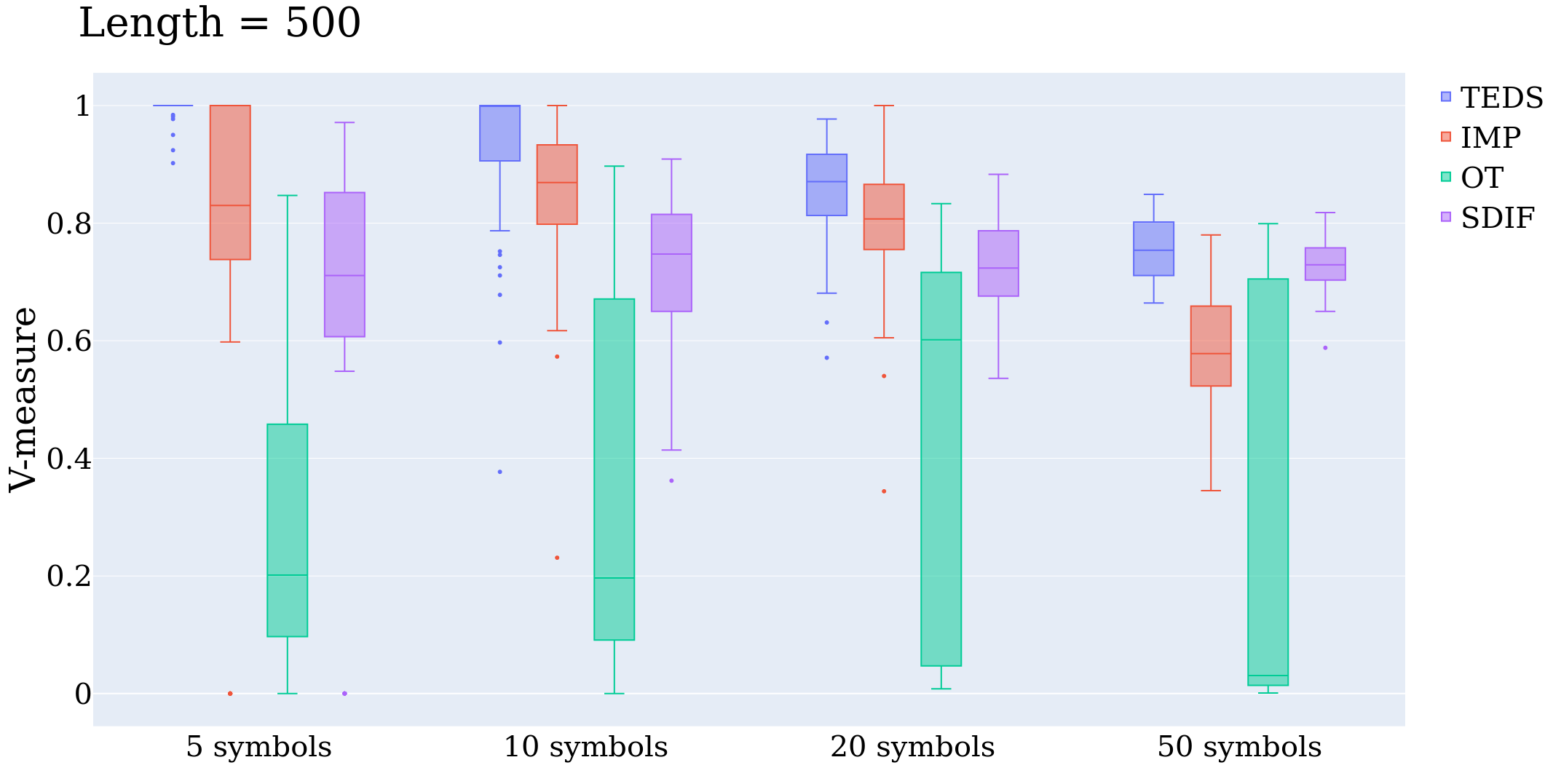
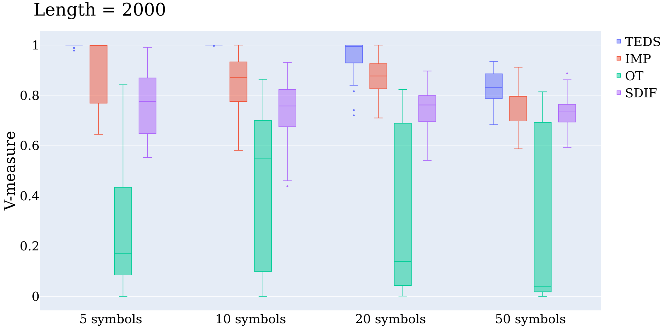
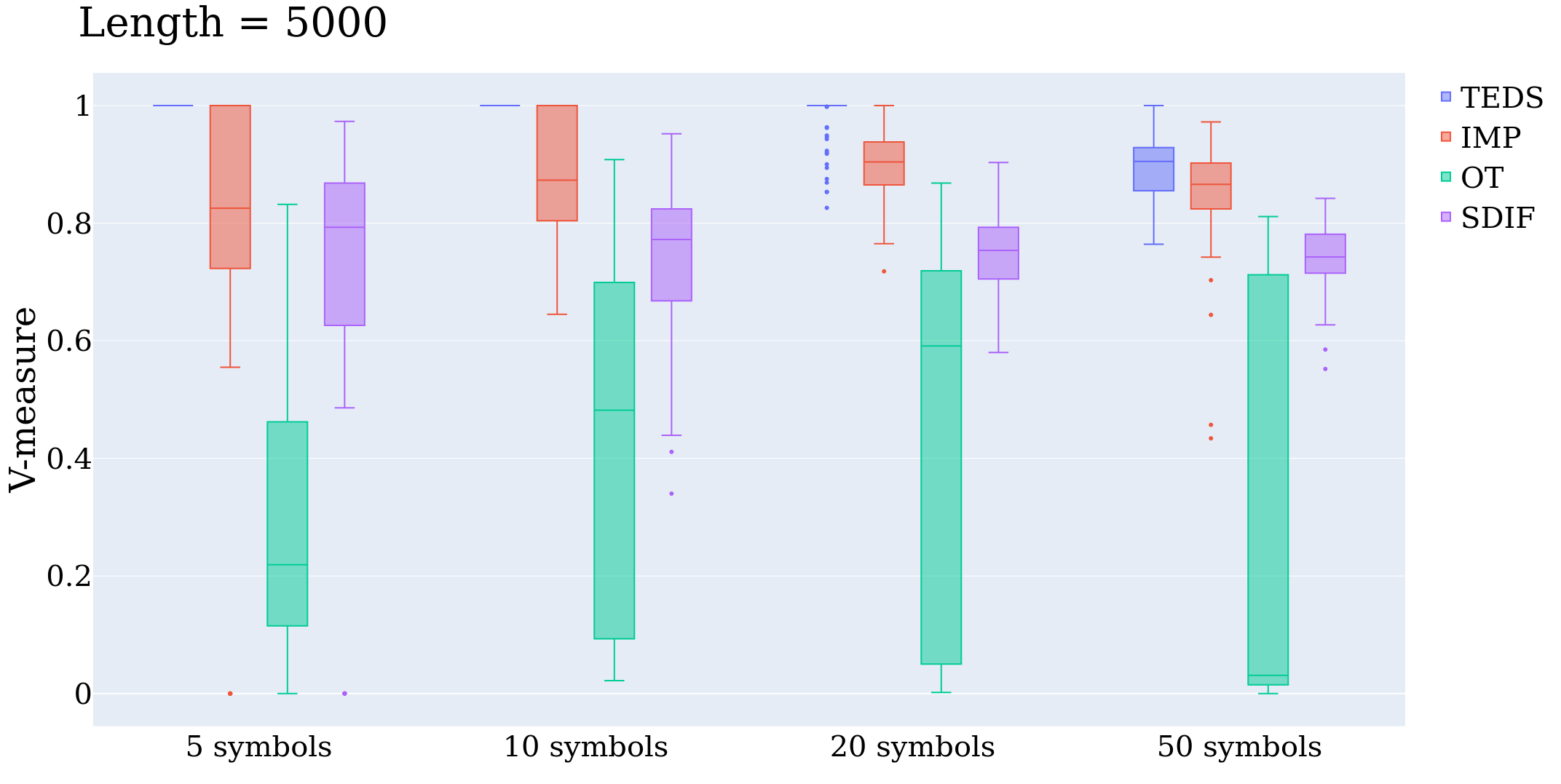
Figure 3: Comparison of the deinterleaving algorithms on synthetic data of size $n=500$, 2000 and 5000. Tests were made for 5, 10, 20 and 50 symbols. Each box represents the distribution of V-measure scores obtained by the different algorithms and computed for 100 independent scenarios.

First we observe that TEDS (in blue) always returns the ground truth partition for the scenarios with 5 and 10 symbols and sequences with 5000 data points (V-measure scores always equal to 1). For other configurations, the number of data points is not sufficient to guarantee a consistent estimation of the score associated to each partition. Unsurprisingly, the worst results are obtained for scenarios with the highest number of symbols, $|\mathcal{A}|=50$, and the lowest numbers of data points, $n=500$.

Overall, we observe that TEDS (in blue) dominates all the competitors for all configurations. The second best algorithm is IMP (in red), which also uses a deinterleaving scheme based on a Markov representation of the data. Algorithms that are not based on a Markov model return symbol partitioning far from the ground truth, as evidenced by the low V-measure scores obtained by SDIF and OT for the different scenarios.

Regarding the computation time required to find the best partition, TEDS and IMP are the algorithms that require the most computing time, because they require the computation of thousands of entropy scores during the exploration of the partition space.

Figure 4 displays the distributions of the number of partitions evaluated by second by each algorithm during the search for sequences of size $n=1000$ with a number of symbols equal to 5, 10, 20 and 50. We observed the same pattern for other size of sequences (500, 2000 an 5000). As shown on this Figure, IMP (in red) is faster when the number of different symbols is low, while TEDS (in blue) becomes faster when the number of symbols increases. When the number of symbols is low, TEDS is slower than IMP because it needs to infer more parameters due to the additional estimation of sojourn times. However, TEDS scales better with the number of symbols (correlated with the number of transmitters in these datasets). It can be explained by the fact that as the number of transmitters increases, the size of each sub-sequence associated with each transmitter decreases on average (for a fix number $n$ of symbols observed in the complete sequence). This enables faster evaluations of the incremental update of the current partition during the search, as the entropies associated with the various independent processes are quicker to evaluate. Conversely, IMP becomes slower as the number of transmitters increases, due to the time required to evaluate the parameters of the Markov switching process $P_{w}$ (cf. Equation (14)), which must be estimated on the complete sequence of observed data and whose complexity increases with the number of different transmitters.

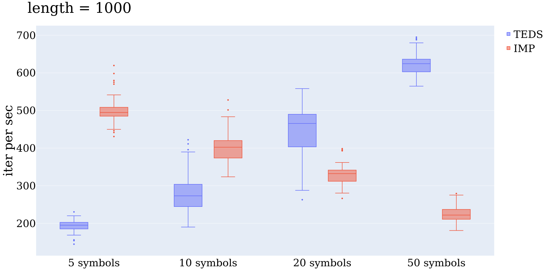
Figure 4: Distributions of the number of partitions evaluated by second by algorithms TEDS and IMP during the search for sequences of size $n=1000$ with a number of symbols equal to 5, 10, 20 and 50.

5.4 Electronic Warfare experiments

In this section we present an application on datasets coming from an Electronic Warfare data generator which simulates realistic situations with an airborne ESM (Electronic Support Measure) receiver in an environment composed of many radars whose number and positions can be selected in the simulation. One configuration corresponds to a random draw in a realistic radar library and a random draw in their relative phasing. For each configuration, a dataset $\mathcal{D}$ consisting in a sequence of intercepted pulse parameters, including their corresponding frequency (CF) and time of arrival (ToA), is generated. The ground truth partition $\Pi_{truth}$ (i.e., the association of each pulse to each transmitter) is given by the simulator but is assumed unknown. The objective is then to retrieve $\Pi_{truth}$ from the data.

5.4.1 Data description

Data are composed of $100$ scenarios generated with the ESM simulator. One scenario, illustrated in Figure 5, corresponds to a manually selected window lasting few seconds in a simulation of several minutes. The windows $\llbracket 0,T\rrbracket$ during which the pulses are observed for each scenario, were selected regarding two criteria: two different transmitters cannot transmits in the same frequency otherwise we are in a case of non disjoint alphabets, and all transmitters cannot cease to transmit in the time window in order to meet as much as possible the hypothesis $(\mathcal{P})$ and $(\mathcal{Q})$ made for the data generating process (see Section 2).

Scenario were generated with or without missing pulses and with or without noises, the missing rate can reach $60\%$ and missing pulses are randomly drawn according to a uniform law.

The length of the sequences observed in the different scenarios ranges from $90$ to $8600$, and the number of transmitters varies from 1 to 11.

5.4.2 Preprocessing step

A preprocessing of the data is first performed to obtain the alphabet $\mathcal{A}$ from the dataset $\mathcal{D}$, as it is done in [7]. It consists in clustering pulses with the DBSCAN algorithm [16] based on their frequency. Then, each cluster obtained is associated with a symbol in $\mathcal{A}$. We then obtain a sequence of frequency symbols $z^{n}$ with their corresponding arrival times $t^{n}$.

The $\epsilon$-neighborhood parameter of DBSCAN corresponds to our precision parameter and is a fixed number of the order of the frequency measured in MHz. After this pulse clustering into the different groups (symbols), we obtain a number of symbols ranging from $7$ to $53$ in the different scenarios.

Figure 5 illustrates an example of data generated with the ESM simulator. Both plots show the frequency of the pulses (y-axis) according to their time of arrival (x-axis). The top image shows the result of the preprocessing step, i.e., pulses grouped into frequency symbols. The bottom image corresponds to the ground truth with the symbols generated by four different transmitters.

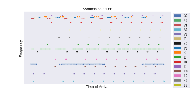
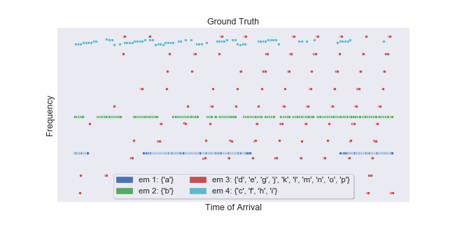
Figure 5: Graphs showing pulse frequency as a function of arrival time. Scales have been hidden on purpose. The upper plot shows the frequency symbols obtained after the pre-processing step: 16 symbols were obtained represented by letters from $a$ to $p$. The bottom plot corresponds to the partition of the letters into four groups (ground truth).

5.4.3 Hyperparameter calibration

We first performed a calibration of the main critical parameters of the different algorithms in order to maximize the average V-measure score on a train set composed of the first 50 instances. With this process, the penalization parameter $\beta$ of TEDS in the score computation (cf. Equation (9)) is set to 19. The penalization parameter $\beta$ of IMP is set to 0.1. Three parameters were optimized for SDIF, $\epsilon=0.05$, threshold $x=0.9$, and a second threshold needed for the PRI (Pulse Repetition Interval) transform, $\alpha=0.5$. For the OT optimal transport algorithm, the hierarchical cluster cut is defined as a function of a silhouette score with a threshold set at $s=0.2$. These parameters are gathered in Table 1.

5.4.4 Validation of the performances

With the calibrated parameters, we ran the compared algorithms on the 50 remaining validation instances. Figure 6 displays the distribution of V-measure scores obtained by the four algorithms for the 50 scenarios.

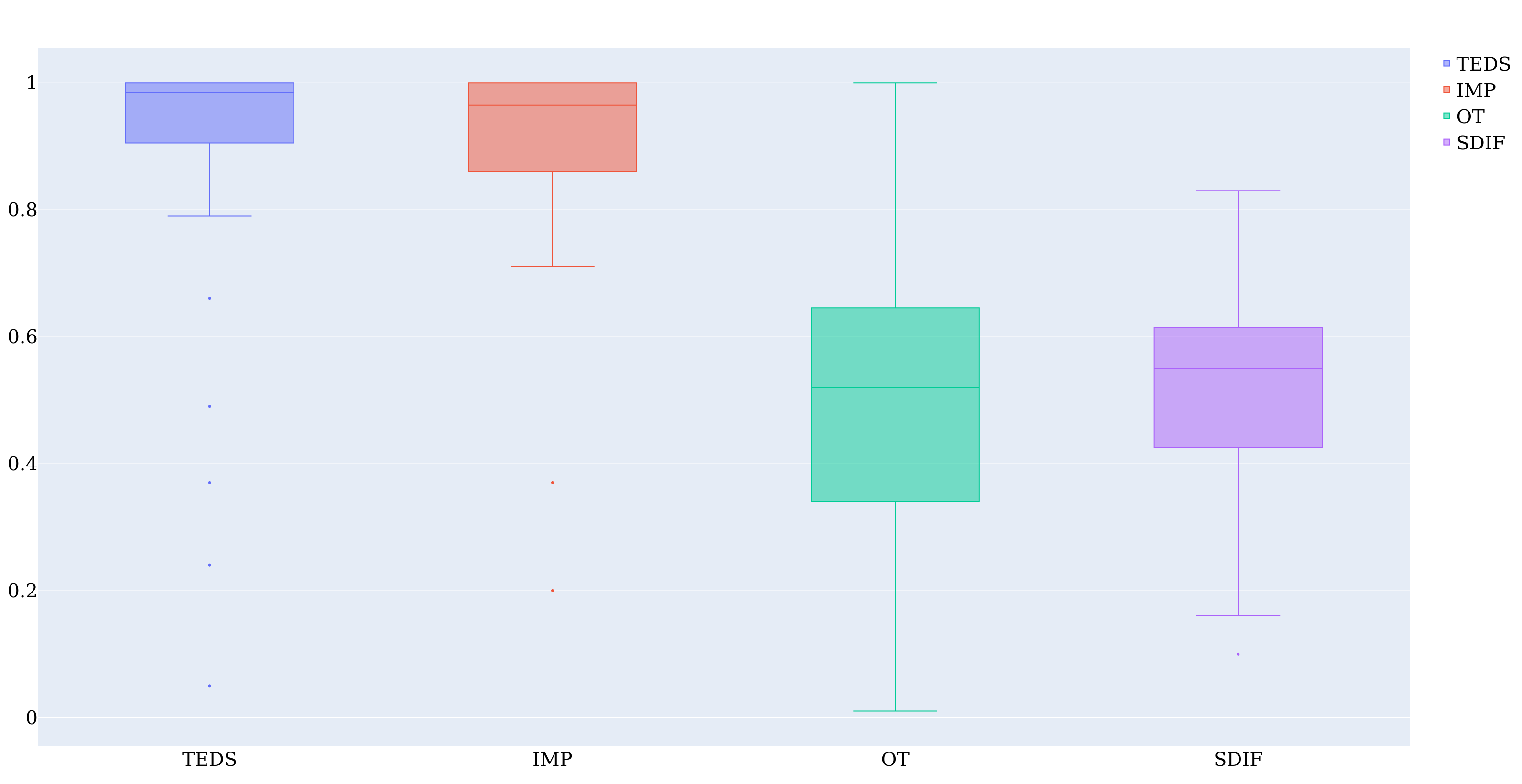
Figure 6: Comparison of deinterleaving algorithm on simulated PDWs. One box represents the distribution of V-measure of the algorithm on the 50 test scenarios.

TEDS and IMP obtains the best results in comparison with the other algorithms, with a slightly better median obtained by TEDS in comparison with IMP, even if a statistical test indicates that the difference in scores between TEDS and IMP is not significant. TEDS returned 17 perfectly deinterleaved scenarios over 50 against 16 for IMP. These two algorithms does not retrieve the ground truth for the same scenarios, which highlights to some extend the complementary nature of these two approaches for this type of data.

6 Discussion and Perspectives

The main contribution of this paper is to propose a new deinterleaving method for interleaved pulse trains, which exploits both entropy minimization of the symbol sequence and entropy minimization of their sojourn times distribution. The choices made in constructing the model (mixture of independent renewal processes, entropy evaluation and penalty term) are supported by theoretical analysis. We have shown that minimizing the proposed score allows us to recover the true partition associated with the generation of the observed sequence in the large sample limit. This theoretical result is confirmed by an experimental analysis of the score consistency. A comparison with other algorithms on synthetic data and electronic warfare data from a realistic simulator confirmed that TEDS is competitive with state-of-the-art algorithms for the deinterleaving task and scales favorably, in terms of computing time required, to the number of transmitters in the generative process.

This work opens up various perspectives for future research. First of all, we have observed that some of the assumptions made in this paper can be violated in reality. In particular, we assumed in this work that the sub-alphabets are disjoint, which is not always the case in realistic scenarios, because different transmitters may send pulse with the same frequency. Secondly, we have assumed that all radars in the environment constantly emit, but it may happen that a radar emits no symbol for an extended period of time. The model could take this into account by introducing, for example, a temporary ”off” state for each radar, during which it emits no pulses.

[Proofs of the main article]

Proof of Theorem 1

Proof.

Let $\Pi^{\prime}$ be a partition such that $P=G_{\Pi^{\prime}}(\{P^{e}\}_{e\in E(\Pi^{\prime})})$. Let us assume that $\Pi\neq\Pi^{\prime}$ and let us show that we arrive at a contradiction. As $\Pi\neq\Pi^{\prime}$, by swapping the role of $\Pi$ and $\Pi^{\prime}$ if required, we claim that there exists a sub-alphabet $A_{e_{\Pi^{\prime}}}\in\Pi^{\prime}$, such that $|A_{e_{\Pi^{\prime}}}|\geq 2$ and $A_{e_{\Pi^{\prime}}}\notin\Pi$. $A_{e_{\Pi^{\prime}}}$ contains at least two symbols $a$ and $b$, such that $a$ is in a sub-alphabet $A_{e_{\Pi}}\in\Pi$ and $b\notin A_{e_{\Pi}}$. Thus, there exists $A_{e^{\prime}_{\Pi}}\in\Pi$, such that, $b\in A_{e^{\prime}_{\Pi}}$ with $A_{e^{\prime}_{\Pi}}\neq A_{e_{\Pi}}$.

We denote by $k_{min}$ the least possible delay between two symbols $a$ that $P$ can generate (i.e., $k_{min}=\underset{k\in K^{a}}{min}(k)$). Since $P=G_{\Pi^{\prime}}(\{P^{e}\}_{e\in E(\Pi^{\prime})})$, $b$ cannot be emitted after $a$ in a time delay lower than $k_{min}$. Since $P=G_{\Pi}(\{P^{e}\}_{e\in E(\Pi)})$, $P$ can generate a sequence $z[A_{e_{\Pi}}\cup A_{e^{\prime}_{\Pi}}]=z_{t_{a}}..z_{t_{b}}..z_{t_{a^{\prime}}}$, with $z_{t_{a}}=a$, $z_{t_{b}}=b$, $z_{t_{a^{\prime}}}=a$, where $t_{a^{\prime}}-t_{a}=k_{\min}$ and $t_{a}<t_{b}\leq t_{a^{\prime}}$, under assumptions $(\mathcal{P})$ and $(\mathcal{Q})$. This is always true since $P^{e_{\Pi}}$ can generate any sub-sequence corresponding to an arbitrary number $\lambda$ of repetitions of symbol $a$, with time delay $k_{min}$ separating each occurrence. For a sufficiently high $\lambda$, $e^{\prime}_{\Pi}$ can emit symbol $b$ during the same interval, whatever $K^{e_{\Pi}}$ and $K^{e^{\prime}_{\Pi}}$.

Thus, either $t_{b}=t_{a^{\prime}}$, which is impossible for $\Pi^{\prime}$ since arrival times of symbols from a single transmitter must be strictly increasing (by definition of a renewal process as given in Section 2.1), or it contradicts the previous assertion that states that $t_{b}-t_{a}\geq k_{min}$, which concludes the proof.

∎

Proofs of Section 3

Proposition 1 The exact log-likelihood function $\text{log}(\mathcal{L}^{T}_{A_{e}}(z^{n}[A_{e}],t^{n}[A_{e}]))$ and the approached likelihood $\text{log}(\bar{\mathcal{L}}^{T}_{A_{e}}(z^{n}[A_{e}],t^{n}[A_{e}]))$ functions are asymptotically equivalent when $T\rightarrow\infty$.

Proof.

According to equation 2 and equation 3:

$$\frac{\text{log}(\mathcal{L}^{T}_{A_{e}}(z^{n}[A_{e}],t^{n}[A_{e}]))-\text{log}(\bar{\mathcal{L}}^{T}_{A_{e}}(z^{n}[A_{e}],t^{n}[A_{e}]))}{\text{log}(\bar{\mathcal{L}}^{T}_{A_{e}}(z^{n}[A_{e}],t^{n}[A_{e}]))}=\frac{\text{log}(P^{e}(z_{0}))+\text{log}(\overline{H}_{z_{N^{e}(T)}}(u_{T}))}{\text{log}(\bar{\mathcal{L}}^{T}_{A_{e}}(z^{n}[A_{e}],t^{n}[A_{e}]))}$$ (15)

We have $0<P^{e}(z_{0})\leq 1$ and $0<\overline{H}_{z_{N^{e}(T)}}(u_{T}))\leq 1$. Moreover, when $T$ goes toward infinity, $\text{log}(\bar{\mathcal{L}}^{T}_{A_{e}}((z^{n}[A_{e}],t^{n}[A_{e}])))\rightarrow\infty$, thus we obtain the result.

∎

Proposition 2 The estimators $\hat{p}^{e}_{i,j}(s^{n})$ and $\hat{q}^{e}_{i,k}(s^{n})$ maximize the approached log-likelihood function $\text{log}(\bar{\mathcal{L}}^{T}_{A_{e}}(z^{n}[A_{e}],t^{n}[A_{e}]))$.

Proof.

This proof is very similar to the proof of Proposition 4.1 in [10]. First we have

$$\forall\ i\ \in A_{e}\ \sum_{k\in K_{i}}q^{e}_{i,k}=1$$ (16)

Let $(\lambda_{i})_{i\in z^{n}[A_{e}]}$ be real coefficients. According to 3 and 16, the approached log-likelihood can be written in the form

$$\text{log}(\bar{\mathcal{L}}^{T}_{A_{e}}(z^{n}[A_{e}],t^{n}[A_{e}]))=\sum_{i,j\in A_{e}}N^{e}_{i,j}(T)\text{log}\ p^{e}_{i,j}+\sum_{i\in A_{e}}\left(\sum_{k\in K_{i}}N^{e}_{i,k}(T)\ \text{log}\ q^{e}_{i,k}+\lambda_{i}(1-\sum_{l\in K_{i}}q^{e}_{i,l})\right)$$ (17)

When deriving Equation 17 with respect to $q^{e}_{i,k}$, we observe that a maximum is obtain in $\hat{q}^{e}_{i,k}=\frac{N^{e}_{i,k}(T)}{\lambda_{i}}$.

By using Equation (16), we obtain

$$1=\sum_{k\in K_{i}}q_{i,k}=\sum_{k\in K_{i}}\frac{N^{e}_{i,k}(T)}{\lambda_{i}}=\frac{1}{\lambda_{i}}\sum_{k\in K_{i}}N^{e}_{i,k}(T)=\frac{N^{e}_{i}(T)}{\lambda_{i}}$$ (18)

Thus, the value of $q^{e}_{i,k}$ maximizing Equation 17 is $\hat{q}^{e}_{i,k}=\frac{N^{e}_{i,k}(T)}{N^{e}_{i}(T)}$. With the same method, we derive that the value of $p^{e}_{i,j}$ maximizing Equation 17 is $\hat{p}^{e}_{i,j}(T)=\frac{N^{e}_{i,j}(T)}{N^{e}_{i}(T)}$.

∎

Proof of Theorem 2

In order to prove Theorem 2, we first show that the generative model $G_{\Pi}$ defined as a set of Markov renewal chains can be represented as an ergodic finite-state-machine (FSM) source.

Using the notation proposed in [6], an FSM over an alphabet $A$ is defined by the triplet $F=(\mathcal{S},s_{0},f)$ where $\mathcal{S}$ is a finite set of states, $s_{0}\in\mathcal{S}$ is a fixed initial state and $f:\mathcal{S}*A\rightarrow{}\mathcal{S}$ is the next-state function. The definition of an FSM source is completed from an FSM with the addition of a conditional probability distribution $P_{F}(.|s)$ with each state $s$ of $\mathcal{S}$, and a probability distribution $P_{F}^{init}(.)$ on the initial state $s_{0}$. The $FSM$ source generates a sequence of states $s^{T}$ by choosing an initial state $s_{0}$ according to $P_{F}^{init}(.)$, then by choosing an action $a_{t}$ according to $P_{F}(.|s_{t-1})$, and transitions to the state $s_{t}=f(s_{t-1},a_{t})$.

.0.1 Markov renewal chain as an FSM

We first observe that a Markov renewal chain $(Z^{e},T^{e})$ can be represented as an FSM source. For a transmitter $e$ generating a sequence of symbols in $A_{e}$, we define the state space $\mathcal{S}^{e}\in A_{e}\times D^{e}$, with $D^{e}$ the set of integers corresponding to the time since a letter of $A_{e}$ has been transmitted. $D^{e}=\{0,1,\dots,\underset{a\in A_{e},k\in K^{a}}{max}k-1\}$ is a finite set of integers.

A state $s^{e}\in\mathcal{S}^{e}$ corresponds to a pair $s^{e}=(z^{e},d)$, with $z^{e}\in A_{e}$, the last symbol transmitted by the emittter $e$ since a duration of $d\in\mathbb{N}$ units of time. We introduce also the set $A^{*}_{e}=A_{e}\cup*$, with $*$ a new symbol, indicating that the previous symbol $z^{e}\in A_{e}$ lasts one unit of time longer but that there is no transition toward a new letter.

For a Markov renewal chain $(Z^{e},T^{e})$, we consider the FSM $\mathcal{F}^{e}=(\mathcal{S}^{e},z^{e}_{0},f^{e})$, with finite state space $\mathcal{S}^{e}\in A_{e}\times D^{e}$, initial state $s^{e}_{0}=(z^{e}_{0},0)\in\mathcal{S}$, and next-state function $f^{e}$ defined as follow. Given a state $s^{e}=(z^{e},d)$ and $a^{e}\in A^{*}_{e}$, we have

$$f^{e}(s^{e},a^{e})=\begin{cases}\text{$(z^{e},d+1)$}&\text{if $a^{e}=*$}\\ \text{$(a^{e},0)$}&\text{if $a^{e}\in A_{e}$}\end{cases}$$

Note that, following a process different from $P^{e}$ on states $S^{e}$ (which we consider in the following for the proof of Theorem 2), it is possible to get actions at state $s^{e}$ that should be unavailable from that state. This is the case for instances when $a^{e}=*$ while $d\geq k_{max}$, with $k_{max}>\max\limits_{a\in A_{e},k\in K^{a}}k$ an arbitrarily delay limit set for the transmitters (allowing to consider finite state sets in the following). In that cases, we consider that $f^{e}(s^{e},a^{e})=s^{e}$ to stay inside $S^{e}$.

To complete the definition of an FSM source, we define a probability $P_{\mathcal{F}^{e}}^{init}(s_{0})=P^{e}(z^{e}_{0})$ of the initial state $s_{0}=(z^{e}_{0},0)$, and for each state $s^{e}=(i,d)$ (with $i\in A_{e}$ and $d\in\mathbb{N}$) and symbol $a^{e}\in A^{*}_{e}$ the conditional distribution

$$P_{\mathcal{F}^{e}}(a^{e}|(i,d))=\begin{cases}\text{$1-h_{i}(d+1)$}&\text{if $a^{e}=*$}\\ \text{$p^{e}_{i,j}h_{i}(d+1)$}&\text{if $a^{e}=j\in A_{e}$},\end{cases}$$

with $h_{i}(t)=\frac{q^{e}_{i,t}}{\sum\limits_{k\in K^{i},k\geq t}q^{e}_{i,k}}$, the instantaneous risk of occurrence of a transition at time $t$ for the letter $i$.

By abuse of notation and for simplicity, we denote $P_{\mathcal{F}^{e}}(s^{e}_{t+1}|s^{e}_{t})=P_{\mathcal{F}^{e}}(a^{e}_{t+1}|s_{t})$ the probability of choosing an action $a_{t+1}$ given $s^{e}_{t}$, which leads to the deterministic transition to the state $s_{t+1}=f(s_{t},a_{t})$.

Proposition 3.

Under assumptions $(\mathcal{Q})$, $(\mathcal{K})$ and $(\mathcal{P})$, each FSM $\mathcal{F}^{e}=(\mathcal{S}^{e},z^{e}_{0},f^{e})$ for $e=1,\dots,E$, is ergodic.

Proof.

Let $K_{e}=\cup_{z\in A_{e}}K^{z}$, the set of all sojourn times for transmitter $e$. Let $K^{z}(d)$ be the set of sojourn times for letter $z$ greater or equal to $d$: $K^{z}(d)=\{k\in K^{z},k\geq d\}$.

First, we observe that all the states $s^{e}\in S^{e}$ of the FSM $\mathcal{F}^{e}=(\mathcal{S}^{e},z^{e}_{0},f^{e})$ built from the Markov renewal chain $(Z^{e},T^{e})$ are recurrent. Indeed, according to assumptions $(\mathcal{Q})$ and $(\mathcal{P})$, for $i,j\in A^{e}$, $l\in\mathbb{N}$ we have $P^{e}(z^{e}_{l+1}=j|z^{e}_{l}=i)>0$, and for $i\in A^{e}$, $k\in K^{i}$, $P^{e}(x_{l+1}=k|z^{e}_{l}=i)>0$. Therefore, for each state $s^{e}=(z^{e},d)\in\mathcal{S}^{e}$, there is always a positive probability to return to this same state $(z^{e},d)$ in a finite number of time steps.

Given a state $(z^{e},d)$, the number of time steps allowing to return to this same state $(z^{e},d)$ with positive probability, is $\Delta T=k^{z^{e}}_{d}+\sum_{i=1,\dots,|K_{e}|}\lambda_{i}k_{i}^{e}$, with $k^{z^{e}}_{d}\in K^{z^{e}}(d)$, $k_{i}^{e}\in K_{e}$ and the $\lambda_{i}$’s are non-negative integer coefficients. Given a state $(z^{e},d)\in\mathcal{S}^{e}$, we denote $T^{e}(z^{e},d)$ this set of transition times $\Delta T$.

Given a state $(z^{e},d)$, let us show that the greatest common divisor (gcd) of the set $T^{e}(z^{e},d)$ is equal to 1.

Let us assume that $gcd(T^{e}(z^{e},d))=m$, with $m>1$ and let us show that we arrive at a contradiction. As $gcd(T^{e}(z^{e},d))=m$,

$$\forall(\lambda_{1},\dots,\lambda_{K_{e}})\in\mathbb{N}^{|K_{e}|},\exists\mu\in\mathbb{N},k^{z^{e}}_{d}+\sum_{i=1,\dots,|K_{e}|}\lambda_{i}k_{i}^{e}=\mu m.$$ (19)

In particular, when all $\lambda_{i}$’s are equal to 0, for $k^{z^{e}}_{d}\in K^{z}(d)$, there exists $\mu_{0}\in\mathbb{N}$, such that $k^{z^{e}}_{d}=\mu_{0}m$. Thus $m$ is a divisor of $k^{z^{e}}_{d}\in K_{e}$.

Given any other sojourn time $k_{i}^{e}\in K_{e}$, such that $k_{i}^{e}\neq k^{z^{e}}_{d}$, using Equation (19), we know that there exists $\mu_{i}$, such that we have also $k^{z^{e}}_{d}+k_{i}^{e}=\mu_{i}m$, and thus we have $k_{i}^{e}=(\mu_{i}-\mu_{0})m$. Then $m$ is a divisor of $k_{i}^{e}$. Thus, $m>1$ is a divisor of all sojourn times $k_{i}^{e}\in K_{e}$, which is impossible because $gcd(K_{e})=1$, according to assumption $(\mathcal{K})$.

Therefore, given a state $(z^{e},d)\in\mathcal{S}^{e}$, we have shown that $gcd(T^{e}(z^{e},d))=1$, thus each state $s^{e}\in\mathcal{S}^{e}$ is aperiodic.

Moreover each pair of states, $s^{e}_{i},s^{e}_{j}\in\mathcal{S}^{e}$, communicate with each other, i.e., when starting from state $s^{e}_{i}$ there is always a positive probability to arrive in state $s^{e}_{j}$ in a finite number of time steps. Therefore, $\mathcal{F}^{e}$ is ergodic. ∎

We now show the likelihood equivalence of both representations (Markov renewal chain and FSM source) for a single transmitter. Let $(z^{e}_{l},t^{e}_{l})_{l=0,\dots,n^{e}-1}$ be sequence of $n^{e}$ symbols $z^{e}\in A_{e}$ with their corresponding time of arrival $t^{e}_{l}\in\mathbb{N}$, generated by $P^{e}$ and observed in the time window $\llbracket 0,T\rrbracket$. Let $s^{e,T}=(s^{e}_{t})_{t=0,\dots,T}$ be the sequence of $T+1$ pairs $s^{e}_{t}\in\mathcal{S}^{e}$, such that $\forall l=0,\dots,n^{e}-1,\forall t\in\llbracket t^{e}_{l},t^{e}_{l+1}\llbracket,s^{e}_{t}=(z^{e}_{l},t-t^{e}_{l})$.

Proposition 4.

The likelihood $L^{T}_{\mathcal{F}^{e}}(s^{e,T})$ of the sequence $s^{e,T}$ generated by the FSM $\mathcal{F}^{e}$ is equal to the likelihood $\mathcal{L}^{T}_{A_{e}}(z^{n^{e}},t^{n^{e}})$ of the sequence $(z^{n^{e}},t^{n^{e}})$ generated by the Markov renewal chain $P^{e}$ until time $T$.

Proof.

The likelihood of the sequence $s^{e}$ observed in the time window $\llbracket 0,T\rrbracket$ is

$$L^{T}_{\mathcal{F}^{e}}(s^{e,T})=P^{e}(z^{e}_{0})\prod_{l=0}^{n^{e}-1}\prod_{t=t^{e}_{l}}^{t^{e}_{l+1}-1}P_{\mathcal{F}^{e}}(s^{e}_{t+1}|s^{e}_{t})\prod_{t=t^{e}_{n^{e}}}^{T-1}P_{\mathcal{F}^{e}}(s^{e}_{t+1}|s^{e}_{t}).$$ (20)

Let us compute separately the terms $\prod_{t=t^{e}_{l}}^{t^{e}_{l+1}-1}P_{\mathcal{F}^{e}}(s^{e}_{t+1}|s^{e}_{t})$ and $\prod_{t=t^{e}_{n^{e}}}^{T-1}P_{\mathcal{F}^{e}}(s^{e}_{t+1}|s^{e}_{t})$.

For $l=0,\dots,n^{e}-1$, given a state $s^{e}_{t^{e}_{l}}=(z^{e}_{l}=i,d=0)$,

$$\prod_{t=t^{e}_{l}}^{t^{e}_{l+1}-1}P_{\mathcal{F}^{e}}(s^{e}_{t+1}|s^{e}_{t}) =[\prod_{t=0}^{t^{e}_{l+1}-t^{e}_{l}-2}1-h_{i}(t+1)]p^{e}_{i,j}h_{i}(t^{e}_{l+1}-t^{e}_{l})$$ (21)

$$=\bar{H}_{i}(t^{e}_{l+1}-t^{e}_{l}-1)p^{e}_{i,j}h_{i}(t^{e}_{l+1}-t^{e}_{l})$$ (22)

with $\overline{H}_{i}(.)$ the survival function of sojourn time in state $i$, defined for $k\in\mathbb{N}$ by

$$\overline{H}_{i}(k)=P(x^{e}_{l+1}>k|z^{e}_{l}=i)=\sum_{k^{i}_{j}\in K^{i},k^{i}_{j}>k}q^{e}_{i,k^{i}_{j}}.$$

Thus,

$$\prod_{t=t^{e}_{l}}^{t^{e}_{l+1}-1}P_{\mathcal{F}^{e}}(s^{e}_{t+1}|s^{e}_{t}) =p^{e}_{i,j}\sum_{k^{i}_{j}\in K^{i},k^{i}_{j}>t^{e}_{l+1}-t^{e}_{l}-1}q^{e}_{i,k^{i}_{j}}\frac{q^{e}_{i,t^{e}_{l+1}-t^{e}_{l}}}{\sum_{k^{i}_{j}\in K^{i},k^{i}_{j}\geq t^{e}_{l+1}-t^{e}_{l}}q^{e}_{i,k^{i}_{j}}}$$ (23)

$$=p^{e}_{i,j}q^{e}_{i,t^{e}_{l+1}-t^{e}_{l}}$$ (24)

$$=P^{e}(z^{e}_{l+1}|z^{e}_{l})\times P^{e}(t^{e}_{l+1}-t^{e}_{l}|z^{e}_{l})$$ (25)

Furthermore, given a state $s^{e}_{t^{e}_{n^{e}}}=(z^{e}_{n^{e}},d=0)$,

$$\prod_{t=t^{e}_{n^{e}}}^{T-1}P_{\mathcal{F}^{e}}(s^{e}_{t+1}|s^{e}_{t}) =\prod_{t=0}^{T-t^{e}_{n^{e}}-1}(1-h_{z^{e}_{n^{e}}}(t+1))$$ (26)

$$=\bar{H}_{z^{e}_{n^{e}}}(T-t^{e}_{n^{e}})$$ (27)

Using equations 20, 23 and 26, we obtain

$$L^{T}_{\mathcal{F}^{e}}(s^{e}) =P^{e}(z_{0})\prod_{l=0}^{{n^{e}}-1}P^{e}(z^{e}_{l+1}|z^{e}_{l})\times P^{e}(t^{e}_{l+1}-t^{e}_{l}|z^{e}_{l})\overline{H}_{z_{n^{e}}}(T-t^{e}_{n^{e}})$$ (28)

$$=\mathcal{L}^{T}_{A^{e}}(z^{n^{e}},t^{n^{e}}).$$ (29)

∎

.0.2 Collection of Markov renewal chains as a FSM

Given a partition $\Pi=\{A_{e_{\Pi}}\}_{e_{\Pi}\in E(\Pi)}$ of $\mathcal{A}$ into $E_{\Pi}$ non-empty and disjoint sub-alphabets, the global generative process $G_{\Pi}$ corresponds to a set of $E_{\Pi}$ independent Markov renewal chains associated to each individual transmitter $e_{\Pi}\in E(\Pi)$, each emitting from its own sub-alphabet $A_{e}$. This process can be represented as a global FSM $\mathcal{F}_{\Pi}=(\mathcal{S}_{\Pi},\mathcal{\textbf{s}}_{0}^{\Pi},f_{\Pi})$, with state set $\mathcal{S}_{\Pi}=\prod_{e\in E(\Pi)}\mathcal{S}^{e}$ corresponding to the cartesian product of the states of the individual FSM of each transmitter $e\in E(\Pi)$ defined in previous section. Given a state $\mathcal{\textbf{s}}\in\mathcal{S}_{\Pi}$, with $\mathcal{\textbf{s}}=\{s^{e}\}_{e\in E(\Pi)}$, and an action $\mathbf{a}\in A^{*}_{\Pi}$, with $A^{*}_{\Pi}=\prod_{e\in E(\Pi)}A^{*}_{e}$ and $\mathbf{a}=(a^{e})_{e\in E(\Pi)}$, we have $f_{\Pi}(\mathcal{\textbf{s}},\mathbf{a})=(f^{e}(s^{e},a^{e}))_{e\in E(\Pi)}$, where $f^{e}$ stands for the next state function from the corresponding individual FSM ${\cal F}^{e}$. For each state we define $P_{\mathcal{F}_{\Pi}}^{init}(\mathbf{s}_{0})=\prod_{e\in E(\Pi)}P_{\mathcal{F}^{e}}^{init}(s^{e}_{0})$ and $P_{\mathcal{F}_{\Pi}}(.|\textbf{s})=\prod_{e\in E(\Pi)}P_{\mathcal{F}^{e}}(.|s^{e})$.

Proposition 5.

Under assumptions $(\mathcal{P})$, $(\mathcal{Q})$ and $(\mathcal{K})$, the FSM $\mathcal{F}_{\Pi}=(\mathcal{S},\mathcal{\textbf{s}}_{0},f)$ is ergodic.

Proof.

Under assumptions $(\mathcal{P})$, $(\mathcal{Q})$ and $(\mathcal{K})$, according to Proposition 3 each FSM $\mathcal{F}^{e}=(\mathcal{S}^{e},z^{e}_{0},f^{e})$ for $e\in E(\Pi)$, is ergodic. Therefore, for $e\in E(\Pi)$, there exists some $n^{e}_{0}$, such that for every integer $n^{e}$, greater than $n^{e}_{0}$, and for every pair of states $i,j\in\mathcal{S}^{e}$, there exists a $i$-to-$j$ path of length $n^{e}_{0}$, as well as a $i$-to-$j$ path of length $n^{e}_{0}+1$ , as well as a $i$-to-$j$ path of length $n^{e}_{0}+2$, and so on. We denote $n_{0}=\underset{e\in E(\Pi)}{max}n^{e}_{0}$. Thus, given any two states $\mathcal{\textbf{s}}_{i}=\{s_{i}^{e}\}_{e\in E(\Pi)}$ and $\mathcal{\textbf{s}}_{j}=\{s_{i}^{e}\}_{e\in E(\Pi)}$, there always exists a path of length $n_{0}$ allowing to reach $\mathcal{\textbf{s}}_{j}$ from $\mathcal{\textbf{s}}_{i}$. Therefore $\mathcal{F}_{\Pi}$ is ergodic. ∎

Given a partition $\Pi=\{A_{e}\}_{e\in E(\Pi)}$ of $\mathcal{A}$ into $E_{\Pi}$ non-empty and disjoint sub-alphabets, let $(z^{n},t^{n})$ be sequence of $n$ symbols $z\in\mathcal{A}$ with their corresponding time of arrival $t_{l}\in\mathbb{N}$, generated by $P=G_{\Pi}$ and observed in the time window $\llbracket 0,T\rrbracket$. In this sequence, each transmitter $e\in E(\Pi)$ generates a sequence $((z^{e}_{l},t^{e}_{l}))_{l=0,\dots,n^{e}-1}$ of $n^{e}$ symbols $z^{e}\in A_{e}$ with their corresponding time of arrival $t^{e}_{l}\in\mathbb{N}$.

Let $\mathbf{s}=(\mathbf{s}_{t})_{t=0,\dots,T}$ be the sequence of $T+1$ states $\mathbf{s}_{t}=\{s^{e}_{t}\}_{e\in E(\Pi)}\in\mathcal{S}_{\Pi}$, such that $\forall e\in E(\Pi),\ \forall l=0,\dots,n^{e}-1,\forall t\in\llbracket t^{e}_{l},t^{e}_{l+1}\llbracket,s^{e}_{t}=(z^{e}_{l},t-t^{e}_{l})$.

Proposition 6.

The likelihood $L^{T}_{\mathcal{F}_{\Pi}}(\mathbf{s})$ of this sequence $\mathbf{s}$, generated by the FSM $\mathcal{F}_{\Pi}$, with probability $P_{\mathcal{F}}^{init}$ of the initial state and transition probabilities $P_{\mathcal{F}_{\Pi}}$, and observed until time $T$, is equal to the likelihood $\mathcal{L}^{T}_{\Pi}(z^{n},t^{n})$ of the sequence $(z^{n},t^{n})$ generated by $P$.

Proof.

This is immediate, as all the transmitters are independent, and using Proposition 4.

∎

Now using Theorem 1 and Propositions 1, 5, 6 we prove Theorem 2.

Proof.

For this proof we took inspiration from the proof of Lemma 10 in [6] and we use the representation of the generative model $G_{\Pi}$ as a global ergodic FSM ${\cal F}_{\Pi}$, as described above.

Let $\Pi^{{}^{\prime}}$ be a partition of $\mathcal{A}$ such that $\Pi^{{}^{\prime}}\neq\Pi$.

Let respectively $\mathcal{F}_{\Pi}=(S_{\Pi},s^{\Pi}_{0},f_{\Pi})$ and $\mathcal{F}_{\Pi^{\prime}}=(S_{\Pi^{\prime}},s^{\Pi^{\prime}}_{0},f_{\Pi^{\prime}})$ be the FSM representing $P_{\Pi}=G_{\Pi}(\{P^{e}\}_{e\in E(\Pi)})$ and $P_{\Pi^{\prime}}=G_{\Pi^{\prime}}(\{P^{e}\}_{e\in E(\Pi^{\prime})})$. Let $P_{\mathcal{F}_{\Pi}}$ and $P_{\mathcal{F}_{\Pi^{\prime}}}$ be the respective probability distribution defined on states of the respective FSM $\mathcal{F}_{\Pi}$ and $\mathcal{F}_{\Pi^{\prime}}$ to represent the processes.

Let $\mathcal{F}^{+}=(S^{+},s^{+}_{0},f^{+})$ be a common refinement of $\mathcal{F}_{\Pi}$ and $\mathcal{F}_{\Pi^{\prime}}$, such that there exist functions $g_{\Pi}:S^{+}\rightarrow S_{\Pi}$ and $g_{\Pi^{\prime}}:S^{+}\rightarrow S_{\Pi^{\prime}}$ allowing to recover states of both processes from $S^{+}$. That is, for any sequence $(z^{n},t^{n})$ observed until time $T$ and its corresponding state sequence $(s^{+}_{t})_{t=0}^{T}$, the respective state sequences $\left(s_{t}^{\Pi}\right)_{t=0}^{T}$ and $\left(s_{t}^{\Pi^{\prime}}\right)_{t=0}^{T}$ satisfy $s_{t}^{\Pi}=g_{\Pi}\left(s_{t}^{+}\right)$ and $s_{t}^{\Pi^{\prime}}=g_{\Pi^{\prime}}\left(s_{t}^{+}\right)$, for any $t=0\dots T$. According to [6], it is always possible to construct a common refinement of two FSMs, whose state set $S^{+}$ is the Cartesian product of the two respective state sets. Thus, for any state $s_{t}^{+}\in S^{+}$, we consider $s_{t}^{+}=(s_{t}^{\Pi},s_{t}^{\Pi^{\prime}})$, with $s_{t}^{\Pi}\in{\cal S}^{\Pi}$ and $s_{t}^{\Pi^{\prime}}\in{\cal S}^{\Pi^{\prime}}$.

At any time step $t$, $s_{t}^{\Pi}\in{\cal S}_{\Pi}$ (resp. $s_{t}^{\Pi^{\prime}}\in{\cal S}_{\Pi^{\prime}}$) can be recovered from $s_{t}^{+}$, by considering the function $g_{\Pi}$ (resp. $g_{\Pi^{\prime}}$) that selects the corresponding part to $\Pi$ (resp. $\Pi^{\prime}$) from $s_{t}^{+}$. In the following, we note $P_{{\cal F}}^{+}$ the adaptation of the probabilities $P_{\cal F}$ to the states of the FSM ${\cal F}^{+}$, that is: $\forall s_{i}^{+}\in{{\cal S}^{+}},\forall a\in A^{*}_{\Pi},P^{+}_{{\cal F}_{\Pi}}(a|s_{i}^{+})=P_{{\cal F}_{\Pi}}(a|g_{\Pi}(s_{i}^{+}))$. Thus, $\forall(s_{i}^{+},s_{j}^{+})\in{{\cal S}^{+}}\times{{\cal S}^{+}},P^{+}_{{\cal F}_{\Pi}}(s_{j}^{+}|s_{i}^{+})=\sum_{a\in A^{*}_{\Pi}}P_{{\cal F}_{\Pi}}(a|g_{\Pi}(s_{i}^{+}))I(f^{+}(s_{i}^{+},a)=s_{j}^{+})$, with $I(.)$ the indicator function. One notes that to make $P^{+}_{{\cal F}_{\Pi}}$ irreducible, we consider in the following a set $S^{+}$ only containing states that are reachable from the process $P_{\Pi}$. Thus, ${\cal S}^{+}$ is a finite state space, since every transmitter owns a finite maximal emission delay. Also, as $P_{\mathcal{F}_{\Pi}}$ is ergodic according to Proposition 3 under assumptions $(\mathcal{P})$, $(\mathcal{Q})$ and $(\mathcal{K})$, and $P^{+}_{{\cal F}_{\Pi}}$ is ergodic under the same assumptions.

In that setting, the asymptotic normalized Kullbak-Liebler divergence relative to $P_{\Pi}$ from $P_{\Pi^{\prime}}$ can be written as:

$$D(P_{\Pi}||P_{\Pi^{\prime}}) = D(P^{+}_{\mathcal{F}_{\Pi}}||P^{+}_{\mathcal{F}_{\Pi^{\prime}}})$$

$$= \sum_{s\in S^{+}}P^{+}_{\mathcal{F}_{\Pi}}(s)D(P^{+}_{\mathcal{F}_{\Pi}}(.|s)||P^{+}_{\mathcal{F}_{\Pi^{\prime}}}(.|s)),$$

with $D(P^{+}_{\mathcal{F}_{\Pi}}(.|s)||P^{+}_{\mathcal{F}_{\Pi^{\prime}}}(.|s))$ the Kullback-Leibler divergence of the conditional distribution $P^{+}_{\mathcal{F}_{\Pi}}(.|s)$ from $P^{+}_{\mathcal{F}_{\Pi}^{\prime}}(.|s)$.

Let $(z^{n},t^{n})$ be sequence of $n$ symbols $z\in\mathcal{A}$ with their corresponding time of arrival $t_{l}\in\mathbb{N}$, generated by $P_{\Pi}$ and observed in the time window $\llbracket 0,T\rrbracket$. In this sequence, each transmitter $e$, generates a sequence $(z^{e}_{l},t^{e}_{l})_{l=0,\dots,n^{e}-1}$ of $n^{e}$ symbols $z^{e}\in A_{e}$ with their corresponding time of arrival $t^{e}_{l}\in\mathbb{N}$. Let $\mathbf{s}^{T}=(\mathbf{s}_{t})_{t=0,\dots,T}$ be the sequence of $T+1$ vector states $\mathbf{s}_{t}\in S+$, corresponding to the generation of $(z^{n},t^{n})$ with $P^{+}_{{\cal F}_{\Pi}}$ on ${\cal F}^{+}$.

Let $\hat{P}^{+}_{\mathcal{F}_{\Pi}}(\mathbf{s}^{T})$ be the probability estimator that maximizes the log-likelihood $\log(\hat{L}^{T,+}_{\mathcal{F}_{\Pi}}(\mathbf{s}^{T}))))=\log(\hat{L}^{T}_{\mathcal{F}_{\Pi}}((g_{\Pi}(\mathbf{s}_{t}))_{t=0}^{T}))$, with corresponding maximum likelihood entropy $H^{T,+}_{\mathcal{F}_{\Pi}}(\mathbf{s}^{T})=-\log(\hat{L}^{T,+}_{\mathcal{F}_{\Pi}}(\mathbf{s}^{T}))))$. We have

$$H^{T,+}_{\mathcal{F}_{\Pi}}(\mathbf{s}^{T})=-\text{log}\ \hat{P}^{init,+}_{\mathcal{F}_{\Pi}}(\mathbf{s}^{0})-\sum_{s,s^{\prime}\in\mathbf{s}^{T}}N_{s,s^{\prime}}(T)\text{log}\ \hat{P}^{+}_{\mathcal{F}_{\Pi}}(s^{\prime}|s),$$

with $N_{s,s^{\prime}}(T)$ the number of transition from state $s\in S^{+}$ to state $s^{\prime}\in S^{+}$ observed in the sequence $\mathbf{s}^{T}$ until time $T$.

We have

$$\frac{1}{T}(H^{T,+}_{\mathcal{F}_{\Pi^{\prime}}}(\mathbf{s}^{T})-H^{T,+}_{\mathcal{F}_{\Pi}}(\mathbf{s}^{T})) =\frac{C}{T}+\sum_{s\in\mathbf{s}^{T}}N_{s}/T\sum_{s^{\prime}\in\mathbf{s}^{T}}[N_{s,s^{\prime}}/N_{s}]\log[\hat{P}^{+}_{\mathcal{F}_{\Pi}}(s^{\prime}|s)/\hat{P}^{+}_{\mathcal{F}_{\Pi^{\prime}}}(s^{\prime}|s)]$$

with $C=\text{log}\hat{P}^{init,+}_{\mathcal{F}_{\Pi}}(\mathbf{s}^{0})-\text{log}\hat{P}^{init,+}_{\mathcal{F}_{\Pi^{\prime}}}(\mathbf{s}^{0})$, a constant that does not depends on $T$.

As $\hat{P}^{+}_{\mathcal{F}_{\Pi}}(\mathbf{s}^{T})$ is the probability estimator that maximizes the likelihood of $\mathbf{s}^{T}$, we have $N_{s}/T=\hat{P}^{+}_{\mathcal{F}_{\Pi}}(s)$ and $N_{s,s^{\prime}}/N_{s}=\hat{P}_{\mathcal{F}_{\Pi}}^{+}(s^{\prime}|s)$, since $\mathbf{s}^{T}$ was generated following $P_{\Pi}$. Thus, we have

$$\frac{1}{T}(H^{T,+}_{\mathcal{F}_{\Pi^{\prime}}}(\mathbf{s}^{T})-H^{T,+}_{\mathcal{F}_{\Pi}}(\mathbf{s}^{T})) =\frac{C}{T}+\sum_{s\in\mathbf{s}^{T}}\hat{P}^{+}_{\mathcal{F}_{\Pi}}(s)\sum_{s^{\prime}\in\mathbf{s}^{T}}\hat{P}_{\mathcal{F}_{\Pi}}^{+}(s^{\prime}|s)\log[\hat{P}_{\mathcal{F}_{\Pi}}^{+}(s^{\prime}|s)/\hat{P}_{\mathcal{F}_{\Pi^{\prime}}}^{+}(s^{\prime}|s)]$$

$$=\frac{C}{T}+D(\hat{P}^{+}_{\mathcal{F}_{\Pi}}||\hat{P}^{+}_{\mathcal{F}_{\Pi^{\prime}}}).$$ (31)

Now since the sequence $\mathbf{s}^{T}$ is generated with probability $P_{\mathcal{F}_{\Pi}}$, we have $D(P^{+}_{\mathcal{F}_{\Pi}}||\hat{P}^{+}_{\mathcal{F}_{\Pi}})\rightarrow 0$ as $T\rightarrow\infty$.

Since $\Pi^{\prime}$ is, by assumption different from $\Pi$, and thus following Theorem 1 incompatible with $P_{\Pi}$, no valid assignment of parameters for ${\cal F}_{\Pi^{\prime}}$ can generate $P_{\Pi}$, and, thus, $P^{+}_{{\cal F}_{\Pi}}$ is not in the set of valid parameters $V(\Pi^{\prime})\subset V^{+}$ for ${\cal F}^{+}_{\Pi^{\prime}}$, with $V^{+}$ the whole set of valid parameters in ${\cal F}^{+}$. As discussed more deeply in [6], we can conclude that $D(P^{+}_{\mathcal{F}_{\Pi}}||\hat{P}^{+}_{\mathcal{F}_{\Pi^{\prime}}})\geq\Delta$, for any constant $\Delta>0$, since $P^{+}_{\mathcal{F}_{\Pi}}$ is ergodic, thus with stationary probabilities greater than zero for any state of ${\cal S}^{+}$, and $\hat{P}^{+}_{\mathcal{F}_{\Pi^{\prime}}}\in V(\Pi^{\prime})$.

As $H^{T,+}_{\mathcal{F}_{\Pi}}(\mathbf{s}^{T})=-\log(\hat{L}^{T,+}_{\mathcal{F}_{\Pi}}(\mathbf{s}^{T}))$ and $H^{T,+}_{\mathcal{F}_{\Pi^{\prime}}}(\mathbf{s}^{T})=-\log(\hat{L}^{T,+}_{\mathcal{F}_{\Pi^{\prime}}}(\mathbf{s}^{T}))$, by using Proposition 1 and 6, we obtain

$$H^{T,+}_{\mathcal{F}_{\Pi}}(\mathbf{s}^{T})-H^{T}_{\Pi}(z^{n},t^{n})\xrightarrow[T\rightarrow\infty]{}0$$ (32)

and

$$H^{T,+}_{\mathcal{F}_{\Pi^{\prime}}}(\mathbf{s}^{T})-H^{T}_{\Pi^{\prime}}(z^{n},t^{n})\xrightarrow[T\rightarrow\infty]{}0.$$ (33)

Now from Equation (.0.2), using (32) and (33), we obtain

$$\frac{1}{T}(H^{T}_{\Pi^{\prime}}(z^{n},t^{n})-H^{T}_{\Pi}(z^{n},t^{n}))\geq\Delta>0\ a.s\ as\ T\rightarrow\infty$$ (34)

For a partition $\Pi$, the penalized maximum likelihood score is

$$C^{T}_{\Pi}(z^{n},t^{n})=H^{T}_{\Pi}(z^{n},t^{n})+\beta E_{\Pi}\text{log}(n),$$ (35)

with $\beta$ a positive constant, $E_{\Pi}$ the number of transmitters associated to the partition $\Pi$, and $n\leq T$. Thus, the term $\frac{\beta E_{\Pi}\text{log}(n)}{T}$ goes toward 0 as $T$ goes toward infinity and from Equation (34) we obtain the expected result

$$\frac{1}{T}(C^{T}_{\Pi^{\prime}}(z^{n},t^{n})-C^{T}_{\Pi}(z^{n},t^{n}))\geq\Delta>0\ a.s\ as\ T\rightarrow\infty,$$ (36)

which concludes the first part of the proof of Theorem 2.

To prove the second part of the Theorem 2, we first start by considering the FSM ${\cal F}^{*}=(S^{*},s_{0}^{*},f^{*})$, which corresponds to the common refinement ${\cal F}^{+}$ in which we remove from $f^{+}$ any transition which are either impossible regarding $\Pi$ or $\Pi^{\prime}$, or that lead to any $s\in{\cal S}^{+}$ from which every sequence to come back in $s$ implies impossible actions regarding $\Pi$ or $\Pi^{\prime}$. Hence, ${\cal S}^{*}\subset{\cal S}^{+}$ contains only states that are reachable following possible transitions for both processes, starting from any state from ${\cal S}^{*}$. By definition $s\in{\cal S}^{*}$ which implies there exists a set of trajectories in ${\cal F}^{*}$ that allows us to go back to $s$. We note $P_{\Pi|\Pi^{\prime}}$ the conditional probability of any sequence $(z^{n},t^{n})$ from $P_{\Pi}$ given that this sequence is possible for a process $P_{\Pi^{\prime}}$ based on $\Pi^{\prime}$. This corresponds to considering $P^{*}_{{\cal F}_{\Pi}}$ as the probabilities from $P^{+}_{{\cal F}_{\Pi}}$ adapted to ${\cal F}^{*}$, where the probability mass of actions leading deterministically outside ${\cal S}^{*}$ from any state in ${\cal S}^{*}$ are evenly redistributed on other admissible actions regarding $f^{*}$.

As already mentioned above, impossible actions for $P_{\Pi^{\prime}}$ can be emitted from $P_{\Pi}$ when for instance an emission delay is lower (resp. greater) than the minimal (resp. maximal) delay for the corresponding transmitters from $\Pi^{\prime}$.

• First, regarding maximal delay, following $P_{\Pi}$ it may happen that a symbol $z$ from a transmitter $e$ of $\Pi$ was not observed since a long time $d$, because for instance other symbols from $e$ were repeated many times after its last occurrence. If that symbol is alone (or with other symbols in the same situation) in its sub-alphabet of $\Pi^{\prime}$, an impossible sequence for $P_{\Pi^{\prime}}$ can occur, if the maximal delay $k_{max}$ for a transmitter is exceeded. We argue that, starting from a state from ${\cal S}^{*}$, there always exists a finite $k_{max}$ sufficiently high to maintain aperiodicity of the state despite these blocked transitions.

• On the other hand, actions can be blocked because they correspond to the simultaneous emission of symbols that shouldn’t be observed at the same timestep, due to the fact they belong to the same sub-alphabet of $\Pi^{\prime}$. We claim that, either there does not exist any alternative from $s\in{\cal S}^{+}$, and hence $s$ does not belong to ${\cal S}^{*}$, or these symbols can be emitted from their corresponding transmitters in $E(\Pi)$ at different timesteps. When such a delayed emission occurs, the corresponding transmitter recovers its whole set of possible delays, with gcd of 1, hence ensuring aperiodicity of the state in ${\cal F}^{*}$.

Thus, we argue that, if ${\cal S}^{*}$ is non-empty (some sequences can be generated by both processes when starting from $s_{0}^{\Pi}$), $P^{*}_{{\cal F}_{\Pi}}$ is ergodic under the same assumptions as above for the ergodicity of $P_{{\cal F}_{\Pi}}$ on ${\cal S}$.

In that setting, the KL divergence relative to $P_{\Pi|\Pi^{\prime}}$ from $P_{\Pi^{\prime}}$ can be given as

$$D(P_{\Pi|\Pi^{\prime}}||P_{\Pi^{\prime}}) = D(P^{*}_{\mathcal{F}_{\Pi}}||P^{*}_{\mathcal{F}_{\Pi^{\prime}}})=D(P^{*}_{\mathcal{F}_{\Pi}}||P^{+}_{\mathcal{F}_{\Pi^{\prime}}})$$

$$= \sum_{s\in S^{+}}P^{*}_{\mathcal{F}_{\Pi}}(s)D(P^{*}_{\mathcal{F}_{\Pi}}(.|s)||P^{*}_{\mathcal{F}_{\Pi^{\prime}}}(.|s)).$$

By following the same methodology as above, we can show that

$$\frac{1}{T}(H^{T,*}_{\mathcal{F}_{\Pi^{\prime}}}(\mathbf{s}^{T})-H^{T,*}_{\mathcal{F}_{\Pi}}(\mathbf{s}^{T}))=C/T+D(\hat{P}^{*}_{\mathcal{F}_{\Pi}}||\hat{P}^{*}_{\mathcal{F}_{\Pi^{\prime}}}).$$ (38)

and thus that:

$$\frac{1}{T}(H^{T}_{\Pi^{\prime}}(z^{n},t^{n})-H^{T}_{\Pi}(z^{n},t^{n}))\geq D(P^{*}_{\mathcal{F}_{\Pi}}||\hat{P}^{+}_{\mathcal{F}_{\Pi^{\prime}}})\ a.s\ as\ T\rightarrow\infty$$ (39)

for any sequence $(z^{n},t^{n})$ generated from $P_{\Pi|\Pi^{\prime}}$. Next, we can notice that $D(P^{*}_{\mathcal{F}_{\Pi}}||\hat{P}^{+}_{\mathcal{F}_{\Pi^{\prime}}})=0$ only if $\forall s\in{\cal S}^{*}$ such that $P^{*}_{\mathcal{F}_{\Pi}}(s)>0$, $D(P^{*}_{\mathcal{F}_{\Pi}}(.|s)||\hat{P}^{*}_{\mathcal{F}_{\Pi^{\prime}}}(.|s))=0$.

With $\Pi\neq\Pi^{\prime}$, we can distinguish two possible settings.

• At least two symbols $z$ and $z^{\prime}$ belong to the same sub-alphabet ${\cal A}_{e_{\Pi}}$ in $\Pi$ and to two respective different sub-alphabets ${\cal A}_{e_{\Pi^{\prime}}}$ and ${\cal A}_{e^{\prime}_{\Pi^{\prime}}}$ in $\Pi^{\prime}$. For any $s\in{\cal S}^{*}$, such that $s_{\Pi}^{e_{\Pi}}=(z^{\prime},d^{\prime})$, with $s_{\Pi}=g_{\Pi}(s)$, and $s_{\Pi^{\prime}}^{e_{\Pi^{\prime}}}=(z,d)$, with $s_{\Pi^{\prime}}=g_{\Pi^{\prime}}(s)$ (i.e., we have $d>d^{\prime}$), $D(P^{*}_{\mathcal{F}_{\Pi}}(.|s)||\hat{P}^{*}_{\mathcal{F}_{\Pi^{\prime}}}(.|s))=0$ implies $P^{*}_{{\cal F}_{\Pi}}(a_{\Pi}^{e_{\Pi}}=z|s)=P^{*}_{{\cal F}_{\Pi^{\prime}}}(a_{\Pi^{\prime}}^{e_{\Pi^{\prime}}}=z|s)$ for any $(a_{\Pi},a_{\Pi^{\prime}})\in{\cal A}^{*}_{\Pi}\times{\cal A}^{*}_{\Pi^{\prime}}$ such that $P^{*}_{{\cal F}_{\Pi}}(a_{\Pi}|s)>0$. This cannot be true for every such state. Two different states $(s,s^{\prime})\in{{\cal S}^{*}}^{2}$ can be equal on $e_{\Pi}$ (i.e, $s_{\Pi}^{e_{\Pi}}={s^{\prime}}_{\Pi}^{e_{\Pi}}$), while having a different value for $e_{\Pi^{\prime}}$ (e.g., $s_{\Pi^{\prime}}^{e_{\Pi^{\prime}}}=(z,d)$ and ${s^{\prime}}_{\Pi^{\prime}}^{e_{\Pi^{\prime}}}=(z,d^{\prime})$, with $d\neq d^{\prime}$). From the definition of the probabilities of actions, which are based on the instantaneous risk of emission, we have: $P^{*}_{{\cal F}_{\Pi^{\prime}}}(a_{\Pi^{\prime}}^{e_{\Pi^{\prime}}}|s)\neq P^{*}_{{\cal F}_{\Pi^{\prime}}}(a_{\Pi^{\prime}}^{e_{\Pi^{\prime}}}|s^{\prime})$. At the same time, since $P^{*}_{{\cal F}_{\Pi}}(a_{\Pi}^{e_{\Pi}}|s)=P^{*}_{{\cal F}_{\Pi}}(a_{\Pi}^{e_{\Pi}}|s^{\prime})$, we can conclude that there exists some state $s\in{\cal S}^{*}$, such that $P^{*}_{{\cal F}_{\Pi}}(a_{\Pi}^{e_{\Pi}}|s)\neq P^{*}_{{\cal F}_{\Pi^{\prime}}}(a_{\Pi^{\prime}}^{e_{\Pi^{\prime}}}|s)$.

• At least two symbols $z$ and $z^{\prime}$ belong to two respective different sub-alphabets ${\cal A}_{e_{\Pi}}$ and ${\cal A}_{e^{\prime}_{\Pi}}$ in $\Pi$ and to the same sub-alphabet ${\cal A}_{e_{\Pi^{\prime}}}$ in $\Pi^{\prime}$. Same manner as above, $P^{*}_{{\cal F}_{\Pi}}(a_{\Pi}^{e_{\Pi}}=z|s)$ cannot be equal to $P^{*}_{{\cal F}_{\Pi^{\prime}}}(a_{\Pi^{\prime}}^{e_{\Pi^{\prime}}}=z|s)$ for all $s$ such that $s_{\Pi}^{e_{\Pi}}=(z,d)$, with $s_{\Pi}=g_{\Pi}(s)$, and $s_{\Pi^{\prime}}^{e_{\Pi^{\prime}}}=(z^{\prime},d^{\prime})$, with $s_{\Pi^{\prime}}=g_{\Pi^{\prime}}(s)$.

Thus, $D(P^{*}_{\mathcal{F}_{\Pi}}||\hat{P}^{+}_{\mathcal{F}_{\Pi^{\prime}}})>0$, for any estimation of probabilities in $\mathcal{F}_{\Pi^{\prime}}$, which concludes the proof.

∎

References

• [1] Chad L. Davies and P. Hollands “Automatic processing for ESM”, 1982
• [2] HK Mardia “New techniques for the deinterleaving of repetitive sequences” In IEE Proceedings F (Radar and Signal Processing) 136.4, 1989, pp. 149–154 IET
• [3] Tanya L Conroy and John B Moore “On the estimation of interleaved pulse train phases” In IEEE Transactions on Signal Processing 48.12 IEEE, 2000, pp. 3420–3425
• [4] Manon Mottier, Gilles Chardon and Frederic Pascal “Deinterleaving and Clustering unknown RADAR pulses” In 2021 IEEE Radar Conference (RadarConf21) Atlanta, GA, USA: IEEE, 2021, pp. 1–6
• [5] Tuğkan Batu, Sudipto Guha and Sampath Kannan “Inferring Mixtures of Markov Chains” In Learning Theory 3120 Berlin, Heidelberg: Springer Berlin Heidelberg, 2004, pp. 186–199
• [6] Gadiel Seroussi, Wojciech Szpankowski and Marcelo J Weinberger “Deinterleaving finite memory processes via penalized maximum likelihood” In IEEE Transactions on Information Theory 58.12 IEEE, 2012, pp. 7094–7109
• [7] Gabriel Ford, Benjamin J Foster and Stephen A Braun “Deinterleaving pulse trains via interleaved Markov process estimation” In 2020 IEEE Radar Conference (RadarConf20), 2020, pp. 1–6 IEEE
• [8] Jean Pinsolle, Olivier Goudet, Cyrille Enderli and Jin-Kao Hao “A Memetic Algorithm for Deinterleaving Pulse Trains” In Evolutionary Computation in Combinatorial Optimization, Lecture Notes in Computer Science 13987 Cham: Springer Nature Switzerland, 2023, pp. 66–81
• [9] Ariana Minot and Yue M. Lu “Separation of interleaved Markov chains” In 2014 48th Asilomar Conference on Signals, Systems and Computers Pacific Grove, CA, USA: IEEE, 2014, pp. 1757–1761
• [10] Vlad Stefan Barbu and Nikolaos Limnios “Semi-Markov chains and hidden semi-Markov models toward applications: their use in reliability and DNA analysis” Springer Science & Business Media, 2009
• [11] Hervé Cardot, Guillaume Lecuelle, Pascal Schlich and Michel Visalli “Estimating finite mixtures of semi-Markov chains: An application to the segmentation of temporal sensory data” In Journal of the Royal Statistical Society Series C: Applied Statistics 68.5 Oxford University Press, 2019, pp. 1281–1303
• [12] Jeremy Young, Anders Høst-Madsen and Eva-Marie Nosal “Deinterleaving of Mixtures of Renewal Processes” In IEEE Transactions on Signal Processing 67.4, 2019, pp. 885–898
• [13] Donald Ervin Knuth “The art of computer programming” Addison-Wesley Reading, MA, 1973
• [14] Yanchao Liu and Qunying Zhang “Improved method for deinterleaving radar signals and estimating PRI values.” In IET Radar, Sonar and Navigation 12.5, 2018, pp. 506–514
• [15] Andrew Rosenberg and Julia Hirschberg “V-Measure: A Conditional Entropy-Based External Cluster Evaluation Measure” In Joint Conference on Empirical Methods in Natural Language Processing and Computational Natural Language Learning, 2007, pp. 410–420
• [16] Martin Ester, Hans-Peter Kriegel, Jorg Sander and Xiaowei Xu “A density-based algorithm for discovering clusters in large spatial databases with noise” In Proceedings of the Second International Conference on Knowledge Discovery and Data Mining 96.34, 1996, pp. 226–231