Quantum entanglement and Bell inequality violation at colliders

Abstract

The study of entanglement in particle physics has been gathering pace in the past few years. It is a new field that is providing important results about the possibility of detecting entanglement and testing Bell inequality at colliders for final states as diverse as top-quark or $\tau$-lepton pairs, massive gauge bosons and vector mesons. In this review, after presenting definitions, tools and basic results that are necessary for understanding these developments, we summarize the main findings—as published up to the end of year 2023. These investigations have been mostly theoretical since the experiments are only now catching up, with the notable exception of the observation of entanglement in top-quark pair production at the Large Hadron Collider. We include a detailed discussion of the results for both qubit and qutrits systems, that is, final states containing spin one-half and spin one particles. Entanglement has also been proposed as a new tool to constrain new particles and fields beyond the Standard Model and we introduce the reader to this promising feature as well.

1   Introduction

An unmistakable feature of quantum mechanics is the inseparable nature of states describing physical systems that have interacted in the past. The entanglement among these states gives rise to correlations among the different parts of these systems that can be stronger than those expected in classical mechanics and are present even after the subsystems are separated and can no longer interact, thus introducing a form of nonlocality in our observations which, however, does not imply any violation of relativity.

Entanglement should not be confused with classical correlations, the latter dealing with intrinsic properties of a system, independently of their measurement. Consider the simplest situation of two spin-1/2 particles that have been prepared in a maximally entangled state, then separated by an arbitrary distance and whose spin is measured with suitable detectors in an arbitrary chosen direction. The result of the measurement is completely random for both detectors, but if one particle is found with spin up, then the second is detected with spin down, and vice versa. As a result, far away though the two daughter particles might be, they must be considered as a single physical entity. This feature represents the phenomenon of quantum nonlocality in a nutshell.

The presence of entanglement leads to the violation of an inequality—named after J. S. Bell, who was first in deriving and discussing it—among the sum of probabilities of the values of certain observables. Whereas the presence of entanglement in itself only confirms the existence of correlations that must be there because of quantum mechanics, the observation of the violation of Bell inequality implies something about the nature of the physical world—namely, its non-separability or, if you prefer, nonlocality—and it represents therefore a profound discovery.

Though the study of entangled states has been an ongoing concern in atomic and solid-state physics for many years, it is only recently that also the high-energy community has taken up in earnest the study of the subject. States in quantum field theory are identified by their mass, momentum and spin (as they are irreducible representations of the Poincarè group) and computations—in the perturbative $S$-matrix framework—are only possible in momentum space; therefore entanglement can only be observed in correlations among the particle spins (or on variables living in the internal flavor space) and it is there that it must be looked for. This looking for, revealing as it does the full quantum state of the final state in a scattering process, has been dubbed quantum state tomography.

Collider detectors, while not designed for probing entanglement, turn out to be surprisingly good in performing this task, thus ushering in the possibility of many interesting new measurements to search for the presence of entanglement as well as to test the violation of Bell inequality. Entanglement has also be shown to provide new tools in probing physics beyond the Standard Model (SM) whenever correlations among the polarizations are accessible from the events.

The extension to the realm of particle physics of the physics of entanglement is not just a reformulation at higher energies of that in atomic physics. New features come into play, most notably, the testing of quantum mechanics beyond electrodynamics with weak and strong interactions, and the presence of states with more than two degrees of freedom as those in the polarization of massive spin 1 particles. Other features pertaining to collider physics will become evident as we proceed in our discussion through the following Sections.

Many aspects and peculiarities of quantum physics are taking more and more central stage in science—from quantum computers to information theory, from theoretical developments to innovative applications. We look at the impact of these developments in the area of high-energy physics. Our aim in writing this review is not broad but rather circumscribed: firstly, we want to present all definitions, tools and basic results that are useful for the study of entanglement and Bell inequality violation at colliders; secondly, we try to summarize the main findings reported in the literature up to the end of 2023. Our hope is to provide an easily accessible collection of resources to serve as springboard for further study.

1.1   The “quantum” in quantum field theory

Quantum field theory, coming as it does from the marriage of quantum mechanics and special relativity, inherits the two main features of quantum mechanics: probabilistic predictions and amplitude interference. To these two, it adds a quantum feature of its own: radiative corrections arising from closed loops in the propagation of the particles (and their creation out of the vacuum). These quantum effects are part of every computation in quantum field theory.

Notwithstanding these features, the feel of a computation in perturbative $S$-matrix is distinctively less “quantum” than in quantum mechanics proper. There is no wave-function collapse and the variables utilized—momenta and occupation number of the asymptotic in- and out-coming states—commute. It is so because the $S$-matrix formulation of quantum field theory is part of a shift that has taken place in particle physics (see [10] for a nice historical discussion) away from the original framework, which was mostly inspired by atomic physics, and toward the typical setting we find at colliders, in which particles come in and go out and we deduce the interactions they have undergone only (at least for elastic processes) by the change in their momenta or (for inelastic scattering processes) also in the occupation numbers—with particles being created or destroyed.

The study of entanglement in particle physics goes against this trend. Entanglement is perhaps the quintessential manifestation of quantum mechanical quirkiness: observations on systems retain a form of correlation even after they have been separated and this correlation implies a nonlocal sharing of resources. There is no way to create an entangled state using local operations and classical communication. A typical example of study of entanglement in a collider setting sees the spin variables as those that are entangled in the scattering and decay processes. Spin variables have been studied until now mostly in the form of classical correlations, which, although sharing some features with entanglement, do not imply entanglement. Quantum tomography, the aim of which is to describe the density matrix of the final state in a scattering process, brings the entanglement among spin variables to center stage.

The presence of nonlocal effects always brings an ominous note to our relativistic ears. Yet there is no reason for concern, for entanglement cannot be used to transfer information between two separated observers. Any information exchange can only be carried by local communication in which relativity is not violated, as it should not since it was incorporated in quantum field theory from the very beginning. Neither is the cluster decomposition (an essential feature of quantum field theory) violated by entanglement. The decomposition has to take place between initial and final states pertaining to two subsets of the $S$-matrix which are then assumed to be far away from one another. Entanglement is present only within the two subsets as long as the relative interactions take place independently of each other.

1.2   Spin correlations at colliders

Spin variables of particles and correlations among them are accessible under the current conditions at colliders only through the study of the distribution of the momenta of the final state into which the original particle decays. These momenta are commuting variables. This fact does not prevent entanglement and Bell inequality violation from being accessible at colliders. The measurement takes place (as we shall see in Section 3) as the polarized particle decays (acting as its own polarimeter) and the momenta of the final state only carry the information into the detectors—in the same way as the momenta of the final electrons carry the information on their spin as their trajectories are separated by the magnetic field in the Stern-Gerlach experiment.

The particles created in the collision first fly through what is (for all practical purposes) a vacuum, going from the collision vertex to hitting the internal surface of the beam pipe and on inside the detector. The characteristic time for this flight is given by the radius of the beam pipe—which is of the order of 1 cm, see, for instance [11]—divided by $c$, for a relativistic particle, that is, $10^{-11}$ s. On the other hand, spin correlations are measured at the time the particle decays, that is, with a characteristic time given by their lifetimes. The particles we are interested in have lifetimes that go from $10^{-25}$ s for the top quark and the weak gauge bosons to $10^{-20}$ s for vector mesons and $10^{-13}$ s for the $\tau$ leptons.

A loss in correlation between the spins of the particles produced at colliders can only take place after they cross into the detector, where the particles would necessarily interact with the atoms of which the detector is made. This interaction never happens since the flight-time inside the beam pipe is much longer than the lifetime of all the particles we are interested in and they decay before reaching the detector proper. For this reason, we can safely assume that the spin correlations we measure are not affected, let alone decorrelated, by the presence of the detector.

The hadronization time scale, a concern only in the case of the top quark, is of the order of $10^{-23}$ s and takes place well after the spin correlations have been measured as the top quark decays.

1.3   The story so far

Helicity and polarization amplitudes at colliders are very sensitive probes into the details of the underlying physics and, for this reason, have been studied for many years and before state quantum tomography. The literature is vast. Older works are reviewed in [12]. More recent contributions introduce the techniques necessary in computing polarizations among fermions [13, 14, 15, 16, 17, 18, 19, 20, 21]), weak gauge bosons [22, 23, 24, 25, 26, 27, 28, 29, 30, 31, 32]) or both [33]. Reconstructing spin-1 polarizations has been well understood since the mid-90s (see [34, 35]) and the framework widely used in experimental analyses like those about heavy meson decays. All these works look for classical correlations and the possibility of measuring them in cross sections or dedicated observables.

Quantum state tomography falls in the same line of inquire of the references above except for the twist of using the polarization amplitudes to define no longer classical but truly quantum correlations. Polarizations are framed in the spin density matrix (as explained in Section 3) and made readily accessible to compute entanglement and Bell operators for the processes of interest.

The violation of the Bell inequality has been tested and verified with experiments measuring the polarizations of photons at low energy (that is, in the range of few eVs) in [36, 37]: two photons are prepared into a singlet state and their polarizations measured along different directions to verify their entanglement and the violation of Bell inequality. More experiments have been performed to further test the inequality [38, 39] and show that the violation takes place also for separations of few kilometers [40]. The Bell inequality has also been tested in solid-state physics [41].

No sooner these tests were reported than ‘loopholes’ were put forward — ways in which, notwithstanding the experimental results, the consequences could be evaded. The presence of these loopholes spurred the experimental community into performing new tests in which the loopholes were systematically closed with photons in [42, 43], using superconducting circuits in [44], and using atoms in [45]. The reader can find more details and references in the older [46] and the more recent [47] review articles.

In particle physics, entanglement with low-energy protons has been probed in [48] and proposed at colliders using hadronic final states in [49], $\tau$ leptons in [50] and discussed in general in [51]. Tests in the high-energy regime of particle physics have been suggested by means of Positronium [52] and Charmonium [53] decays and neutrino oscillations [54] (see also [55] and references therein). A Bell inequality is violated in neutral kaon oscillations due to direct $CP$ violation [56, 57, 58] (see also [59]). Flavor oscillations in neutral $B$-mesons have been argued to imply the violation of Bell inequality [60] (see also [61]). Entanglement among partons in scattering processes of nucleons has recently been studied (see, for instance, [62, 63]). A discussion of entanglement in particle physics also appears in [64, 65].

The interest has been revived recently after entanglement has been convincingly argued [66] (see also [67, 68]) to be present in top-quark pair production at the Large Hadron Collider (LHC) and it was shown that Bell inequality violation is experimentally accessible in the same system and in the decay of the Higgs boson into two charged gauge bosons [69]. The ATLAS Collaboration has found [70] that entanglement is present with a significance of more than $5\sigma$ in top-quark pairs produced near threshold at the LHC.

A sizable body of works has been published since. We review it in the Sections 4 and 5 by organizing it into systems that are qubits and qutrits, that is, entanglement among particles of spin 1/2 and 1. The possibility of using entanglement in probing new physics is reviewed in Section 7. Before doing that, we introduce in Sections 2 and 3 the definitions and tools necessary in the analysis.

2   Entanglement and Bell locality

2.1   Quantum states and observables

In quantum mechanics, the description of a quantum system $S$, for simplicity taken to be finite dimensional ($n$-level system), is realized by means of an ($n$-dimensional) Hilbert space $\mathcal{H}_{n}$, isomorphic to $\mathbb{C}^{n}$, where $\mathbb{C}$ is the set of complex numbers, and by the algebra $M_{n}(\mathbb{C})$ of $n\times n$ complex matrices. The elements $|\psi\rangle$ of $\mathcal{H}_{n}$, normalized to unity, represent states of $S$, while the Hermitian matrices in $M_{n}(\mathbb{C})$, $\mathcal{\hat{O}}^{\dagger}=\mathcal{\hat{O}}$, correspond to system observables, whose mean values, $\langle\mathcal{\hat{O}}\rangle\equiv\langle\psi|\mathcal{\hat{O}}|\psi\rangle$, are statistically linked to measurements of $\mathcal{\hat{O}}$.

The elements of $\mathcal{H}_{n}$ are however just a particular class of states of $S$, those called pure states. In general, the information on $S$ is incomplete and a set of probabilities $\{p_{i}\}$, with $\sum_{i}p_{i}=1$, weights the possible (normalized but not necessarily orthogonal) states of the system $|\psi_{i}\rangle$, $i=1,2,\ldots,m$. In this case, the mean value of any given system observable $\mathcal{O}$ can be expressed as the combination of the pure state mean values $\langle\psi_{i}|\mathcal{\hat{O}}|\psi_{i}\rangle$, weighted with the corresponding probability of occurrence:

$$\langle\mathcal{\hat{O}}\rangle=\sum_{i=1}^{m}p_{i}\,\langle\psi_{i}|\mathcal{\hat{O}}|\psi_{i}\rangle\ .$$ (2.1)

It is then natural to describe the statistical mixture $\{p_{i},|\psi_{i}\rangle\}$ by means of the density matrix:

$$\rho=\sum_{i=1}^{m}p_{i}\,|\psi_{i}\rangle\langle\psi_{i}|\ ,\quad{\rm with}\quad p_{i}\geq 0\ ,\quad{\rm and}\quad\sum_{i=1}^{m}p_{i}=1\ ,$$ (2.2)

where the conditions on the set $\{p_{i}\}$ are those of an ensemble of statistical weights. The average value of an observable $\mathcal{O}$ can then be most simply expressed as

$$\langle\mathcal{\hat{O}}\rangle={\rm Tr}\big{[}\rho\,\mathcal{\hat{O}}\big{]}\ ,$$ (2.3)

where the trace operation of any matrix $X\in M_{n}(\mathbb{C})$ is explicitly given by ${\rm Tr}[X]\equiv\sum_{i=1}^{n}\langle\varphi_{i}|X|\varphi_{i}\rangle$, with the collection of states $\{|\varphi_{i}\rangle\}$ being any orthonormal basis in $\mathcal{H}_{n}$.

From its definition (2.2), any density matrix $\rho$ must satisfy the following three characteristic properties:

• $\rho$ is an Hermitian operator, $\rho^{\dagger}=\rho$,

• $\rho$ is normalized, ${\rm Tr}[\rho]=1$,

• $\rho$ is a positive semi-definite matrix, i.e. $\langle\psi|\rho|\psi\rangle\geq 0$; for all $|\psi\rangle\in\mathcal{H}_{n}$,

in order to preserve the physically consistent interpretation of $\rho$.

Quantum states are thus positive, normalized operators, with the pure states $|\psi\rangle$ represented by projectors $|\psi\rangle\langle\psi|$, as the statistical mixture in (2.2) reduces in this case to a single element. As a consequence, the eigenvalues of density matrices representing pure states are $1$ (non-degenerate) and $0$ ($n-1$ times degenerate), while those, $\{\lambda_{i}\}$, $i=1,2,\ldots,n$, of a generic density matrix $\rho$ are such that: $0\leq\lambda_{i}\leq 1$, with $\sum_{i}\lambda_{i}=1$. It follows that in general: ${\rm Tr}[\rho^{2}]\leq 1$, reaching the upper bound only when $\rho$ is a pure state. Therefore, a quantum state represented by a density matrix $\rho$ is a pure state if and only if $\rho$ is a projector:

$$\rho^{2}=\rho\ ,\qquad{\rm Tr}[\rho^{2}]=1\ .$$ (2.4)

The decomposition of any density matrix $\rho$ in terms of its eigen-projectors $|\lambda_{i}\rangle\langle\lambda_{i}|$, constructed with its eigenvectors $|\lambda_{i}\rangle$, gives its spectral decomposition:

$$\rho=\sum_{i=1}^{m}\lambda_{i}\,|\lambda_{i}\rangle\langle\lambda_{i}|\ ,\quad{\rm with}\quad\sum_{i=1}^{m}\lambda_{i}=1\ ,\quad{\rm and}\quad\langle\lambda_{i}|\lambda_{j}\rangle=\delta_{ij}\ ;$$ (2.5)

the set $\{\lambda_{i}\}$ of eigenvalues of $\rho$ constitutes a probability distribution which completely defines the statistical properties of the quantum state. Although the spectral decomposition (2.5) is unique, it should be stressed that there are infinitely many ways of expressing a density matrix as a linear combination of projectors as in (2.2).

The set of all density matrices describing a quantum system $S$ forms a convex subset of $M_{n}(\mathbb{C})$, as combining different density matrices $\eta_{i}$ into a convex combination $\sum_{i}r_{i}\eta_{i}$, with weights $r_{i}\geq 0$, and $\sum_{i}r_{i}=1$, gives again a density matrix. Pure states are extremal elements of this set, that is they cannot be expressed as a convex combination of other density matrices; they can be used to decompose non-pure states, see (2.2), and indeed in this way they generate the whole set of density matrices.

Any transformation of the system $S$ can be modeled as a linear map acting on the space of density matrices, $\rho\to\mathbb{E}[\rho]$. The most general form of such transformations, as allowed by the statistical interpretation of quantum mechanics outlined above, is given by the following operator-sum representation:

$$\rho\to\mathbb{E}[\rho]=\sum_{i}V_{i}\,\rho\,V_{i}^{\dagger}\ ,$$ (2.6)

for some collection of operators $\{V_{i}\}$. Clearly, the map $\mathbb{E}$ in (2.6) preserves the hermiticity and positivity of $\rho$, and, provided $\sum_{i}V_{i}^{\dagger}V_{i}=\mathbf{1}_{n}$, with $\mathbf{1}_{n}\in M_{n}(\mathbb{C})$ the identity matrix, also its normalization; such a map is called a quantum operation, or simply a quantum channel.

In particular, the unitary dynamics, $\rho\to\mathbb{U}_{t}[\rho]$, generated by a system Hamiltonian operator $H\in M_{n}(\mathbb{C})$, is of the form (2.6), with just one operator $V_{i}$:

$$\rho\to\mathbb{U}_{t}[\rho]=e^{-itH}\,\rho\,e^{itH}\ .$$ (2.7)

The set of transformations $\{\mathbb{U}_{t}\}$ forms a one-parameter group of linear maps, $\mathbb{U}_{t}\circ\mathbb{U}_{s}=\mathbb{U}_{t+s}$, for all $t,s\in\mathbb{R}$, reflecting the reversible character of the unitary Schrödinger dynamics; as such, it preserves the spectrum and the purity of the density matrix:

$$\rho=\rho^{2}\implies\big{(}\mathbb{U}_{t}[\rho]\big{)}^{2}=\mathbb{U}_{t}[\rho]\ .$$ (2.8)

Another common transformation affecting quantum states involves measurement. Assuming the system $S$ be initially prepared in a pure state $|\psi\rangle\langle\psi|$, after measuring a non-degenerate observable $\mathcal{O}=\sum_{k}\mathcal{O}_{k}|k\rangle\langle k|$, expressed in its spectral form with $\mathcal{O}_{k}$ being its eigenvalues and $|k\rangle$ the corresponding eigenvectors, then the outcome $\mathcal{O}_{k}$ occurs with probability $w_{k}=|\langle k|\psi\rangle|^{2}$ and, if the measure indeed produces $\mathcal{O}_{k}$, then the post-measurement system state is the projector $P_{k}=|k\rangle\langle k|$. By repeating the measure operation on copies of the system $S$ equally prepared in the state $|\psi\rangle\langle\psi|$, the collection of the resulting post-measurement states is described by the statistical mixture $\{w_{k},|k\rangle\}$:

$$|\psi\rangle\langle\psi|\to\sum_{k}w_{k}P_{k}=\sum_{k}P_{k}\,\big{(}|\psi\rangle\langle\psi|\big{)}\,P_{k}\ .$$ (2.9)

This transformation can be extended by linearity to cover any initial density matrix $\rho$ for the system $S$; as a result, after the given set of measurements the system state is subjected to the transformation:

$$\rho\to\mathbb{P}[\rho]=\sum_{k}P_{k}\,\rho\,P_{k}\ .$$ (2.10)

Contrary to the unitary dynamics $\mathbb{U}_{t}$, the map $\mathbb{P}$ generally transforms pure states into mixtures, thus involving decoherence effects resulting in the suppression of any initially present phase-interference. This happens because the quantum operation $\mathbb{P}$ effectively describes $S$ as an open system, in this case as a system interacting with the apparatus used to measure the observable $\mathcal{O}$. Quite in general, dynamics generating noise and dissipation through decoherence can be modelled as those of systems in interaction with large external environments; their evolution must be of the form (2.6), the only one guaranteeing physical consistency in any situation.

2.2   Quantum correlations

One of the characteristic properties of quantum mechanics is the possibility of having correlations among constituent quantum systems, that is, correlations among their observables, that cannot be accounted for by classical physics. Initially dismissed as a pure curiosity, the presence of such quantum correlations, that is of entanglement [2, 71, 72], has rapidly become a fundamental resource in the development of disciplines like quantum information and technology, as it allows the implementation of protocols and the realization of various apparatus outperforming classical ones [73, 8].

Many experiments have shown the presence of quantum correlations in various quantum systems involving photons, atoms and more recently elementary particles. Indeed, as entanglement is most likely to emerge as the result of a direct interaction among the constituents of a quantum system, the interaction among elementary particles as seen at colliders seems a promising place to study effects of quantum correlations.

In the following we shall merely deal with bipartite composite quantum systems $S=S_{A}+S_{B}$ consisting of two finite-dimensional parties $S_{A}$ and $S_{B}$, usually identified with two distant, well-separated quantum systems. An observable $\hat{\mathcal{O}}$ of $S$ can then be expressed in a tensor product form, $\hat{\mathcal{O}}=\hat{\mathcal{O}}_{A}\otimes\hat{\mathcal{O}}_{B}$, where $\hat{\mathcal{O}}_{A}$, $\hat{\mathcal{O}}_{B}$ are observables of $S_{A}$ and $S_{B}$, respectively; notice that $\hat{\mathcal{O}}$ is the product of two local operators, $\hat{\mathcal{O}}_{A}\otimes{\bf 1}_{B}$ and ${\bf 1}_{A}\otimes\hat{\mathcal{O}}_{B}$.

A state (density matrix) $\rho$ of $S$ is called separable if and only if it can be written as a linear convex combination of tensor products of density matrices:

$$\rho=\sum_{ij}p_{ij}\,\rho^{(A)}_{i}\otimes\rho^{(B)}_{j}\ ,\quad\text{with}\quad p_{ij}>0\quad\text{and}\quad\sum_{ij}p_{ij}=1\ ,$$ (2.11)

where $\rho^{(A)}_{i}$ and $\rho^{(B)}_{j}$ are density matrices for the subsystems $S_{A}$ and $S_{B}$. States $\rho$ that cannot be written in the form of (2.11) are called entangled or non-separable, and exhibit quantum correlations.

Notice that, by expressing the density matrices $\rho^{(A)}_{i}$ and $\rho^{(B)}_{j}$ in terms of their spectral decomposition, that is in terms of their respective eigenprojectors, separable states as in (2.11) can always be written as linear convex combinations of tensor products of pure states. These states carry statistical correlations, but they are just of classical nature, reflecting the way the pure states are mixed together. Specifically, a separable state of $S$ of the form

$$\rho=\sum_{ij}\lambda_{ij}\,|\psi^{(A)}_{i}\rangle\langle\psi^{(A)}_{i}|\otimes|\psi^{(B)}_{j}\rangle\langle\psi^{(B)}_{j}|\ ,\quad{\rm with}\quad\lambda_{ij}>0\quad{\rm and}\quad\sum_{ij}\lambda_{ij}=1\ ,$$ (2.12)

describes a statistical ensemble that can always be viewed as $N_{ij}$ instances of a system with state vector $|\psi^{(A)}_{i}\rangle\otimes|\psi^{(B)}_{j}\rangle$ coming from a “source” that has “emitted” a total number $N$ of such systems, the ratio $N_{ij}/N$ approaching the weight $\lambda_{ij}$ in the large-$N$ limit. Therefore, in this case the weights $\lambda_{ij}$ just reflect the statistics of the source, viewed as a classical stochastic variable.

In addition, due to the structure of (2.11), the local character of separable states cannot be modified by local actions of the form $\hat{\mathcal{O}}_{A}\otimes\hat{\mathcal{O}}_{B}$ with $\hat{\mathcal{O}}_{A}$, $\hat{\mathcal{O}}_{B}$ admissible quantum operations for the subsystems $S_{A}$, $S_{B}$. In other words, in order to change the local character of a separable state into a nonlocal one, a nonlocal action involving both parties, for instance a direct interaction, is necessary.

Pure, separable density matrices, such that $\rho^{2}=\rho$, are projectors onto state vectors in product form, $|\psi\rangle=$ $|\psi^{(A)}\rangle\otimes|\psi^{(B)}\rangle$, $\rho=|\psi\rangle\langle\psi|$, for some vector states $|\psi^{(A)}\rangle$ of $S_{A}$ and $|\psi^{(B)}\rangle$ of $S_{B}$. Nevertheless, given a generic state vector for the system $S$,

$$|\psi\rangle=\sum_{ij}\psi_{ij}\,|i\rangle^{(A)}\otimes|j\rangle^{(B)}\ ,$$ (2.13)

with $\{|i\rangle^{(A)}\}$, $\{|i\rangle^{(B)}\}$, orthonormal bases in $S_{A}$, $S_{B}$, proving that it can or cannot be written in product form is in general a nontrivial task. Fortunately, the problem can be solved using the Schmidt decomposition [73]; in fact, for any generic state (2.13), one can always find two suitable orthonormal bases for $S_{A}$ and $S_{B}$ yielding a diagonal decomposition:

$$|\psi\rangle=\sum_{k=1}^{d}\lambda_{k}\,|k\rangle^{(A)}\otimes|k\rangle^{(B)}\ ,$$ (2.14)

with non-negative Schmidt coefficients $\lambda_{k}$ and $d$ the lowest dimension among $S_{A}$ and $S_{B}$; if at least two of these coefficients are nonvanishing, the state $|\psi\rangle$ is not in product form and thus it is entangled. As a consequence, denoting with $\rho_{A}={\rm Tr}_{B}[|\psi\rangle\langle\psi|]$, and $\rho_{B}={\rm Tr}_{A}[|\psi\rangle\langle\psi|]$, the partial traces over $S_{B}$ and $S_{A}$ degrees of freedom, respectively, a generic pure state $|\psi\rangle$ of $S$ is separable if and only if its reduced states $\rho_{A}$ and $\rho_{B}$ are pure.

Alternatively, one can focus on the von Neumann entropy, that for a generic density matrix $\rho$ is defined as [73]

$${\cal S}[\rho]=-{\rm Tr}[\rho\ln\rho]\ ;$$ (2.15)

it is the quantum analogue of the classical Shannon entropy. In terms of the reduced density matrices, one can then define the quantity

$$\mathscr{E}[\rho]\equiv-{\rm Tr}[\rho_{A}\ln\rho_{A}]=-{\rm Tr}[\rho_{B}\ln\rho_{B}]\ ;$$ (2.16)

clearly, a pure state $\rho=|\psi\rangle\langle\psi|$ is entangled if and only if its reduced density matrices have non-zero entropy. The quantity $\mathscr{E}[\rho]$, often called in the literature entropy of entanglement, is an entanglement quantifier; assuming for the two systems $S_{A}$ and $S_{B}$ have the same dimension $d$, one finds $0\leq\mathscr{E}[\rho]\leq\ln d$. The first equality holds if and only if the bipartite pure state is separable, while the upper bound is reached by a maximally entangled state,

$$|\Psi_{+}\rangle=\frac{1}{\sqrt{d}}\sum_{i=1}^{d}|i\rangle^{(A)}\otimes|i\rangle^{(B)}\ .$$ (2.17)

When the state $\rho$ of the compound system $S$ is a generic density matrix, deciding whether the state is entangled or not, or quantifying its entanglement content is in general a hard problem [74, 75] and only partial answers are available. In general, one can only rely on so-called entanglement witnesses, quantities that give sufficient conditions for the presence of entanglement in the system.

In building such witnesses, a crucial role is played by positive maps $\Lambda$, that is by linear transformations on the space of matrices, mapping positive matrices, that is, matrices with non-negative eigenvalues, into positive matrices. Let us assume for simplicity that as before two systems $S_{A}$ and $S_{B}$ have the same dimension $d$; then the following basic result holds [76]:

A state $\rho$ of the bipartite system $S$ is entangled if and only if there exists a positive map $\Lambda_{A}$ on the subsystem $S_{A}$, such that the matrix $\rho$ is not left positive by the action of the compound map $\Lambda_{A}\otimes{\bf 1}_{B}$, that is $(\Lambda_{A}\otimes{\bf 1}_{B})[\rho]\ngeq 0$.

A well known, easily implementable entanglement test based on this result involves the transposition map, for instance on the subsystem $S_{A}$: the compound operation $T_{A}\otimes{\bf 1}_{B}$, is called partial transposition; then (Peres-Horodecki criterion) [77]:

A state $\rho$ of the bipartite system $S$ is entangled if it does not remain positive under partial transposition, $(T_{A}\otimes{\bf 1}_{B})[\rho]\ngeq 0$.

It turns out that this entanglement criterion is exhaustive in lower dimensions, for a bipartite system consisting two qubits, or a qubit and a qutrit [78]. In addition, quite in general, the absolute sum of the negative eigenvalues of a partially transposed state, called negativity, can be used to quantify its entanglement content [2].

The relationship between the entropy of the system and of its parts can be used to check whether the state is entangled; if the state $\rho$ is separable, than necessarily: ${\cal S}[\rho]\geq{\cal S}[\rho_{A}]$ and ${\cal S}[\rho]\geq{\cal S}[\rho_{B}]$, where as before $\rho_{A}$ and $\rho_{B}$ are the reduced density matrices [2].

In applications, entanglement witnesses that can be easily computed are needed: a relevant example of such a witness is concurrence. Consider again the bipartite quantum system $S$, made of two $d$-dimensional subsystems $S_{A}$, $S_{B}$, described by a normalized pure state $|\psi\rangle$, or equivalently by the density matrix $|\psi\rangle\langle\psi|$. The concurrence of the system is defined by [79, 80, 81]

$$\mathscr{C}[|\psi\rangle]\equiv\sqrt{2\left(1-{\rm Tr}\big{[}(\rho_{A})^{2}\big{]}\right)}=\sqrt{2\left(1-{\rm Tr}\big{[}(\rho_{B})^{2}\big{]}\right)}\ .$$ (2.18)

As already remarked, any mixed state $\rho$ of the bipartite system can be decomposed into a set of pure states $\{|\psi_{i}\rangle\}$,

$$\rho=\sum_{i}p_{i}\,|\psi_{i}\rangle\langle\psi_{i}|\ ,\quad{\rm with}\quad p_{i}\geq 0\ ,\quad{\rm and}\quad\sum_{i}p_{i}=1\ ;$$ (2.19)

its concurrence is then defined by means of the concurrence of the pure states appearing in the decomposition through an optimization process:

$$\mathscr{C}[\rho]=\underset{\{|\psi\rangle\}}{\rm inf}\sum_{i}p_{i}\,\mathscr{C}[|\psi_{i}\rangle]\ ,$$ (2.20)

where the infimum is taken over all the possible decompositions of $\rho$ into pure states. For a pure state the concurrence (2.18) vanishes if and only if the state is separable, $|\psi\rangle=|\psi_{A}\rangle\otimes|\psi_{B}\rangle$, reaching its maximum value when $\rho$ is a projection on the pure, maximally entangled state (2.17). As the same holds for mixed states [82], the concurrence appears to be a good entanglement detector. Unfortunately, the optimization problem appearing in (2.20) makes the evaluation of the concurrence a very hard mathematical task, with a simple analytic solution only for two-level systems, $d=2$.

Indeed, in this special low-dimensional case, given a two-qubit, $4\times 4$ density matrix $\rho$ as in (2.38), its concurrence can be explicitly constructed using the auxiliary matrix

$$R=\rho\,(\sigma_{y}\otimes\sigma_{y})\,\rho^{*}\,(\sigma_{y}\otimes\sigma_{y})\,,$$ (2.21)

where $\rho^{*}$ denotes the matrix with complex conjugated entries. Although non-Hermitian, the matrix $R$ possesses non-negative eigenvalues; denoting with $r_{i}$, $i=1,2,3,4$, their square roots and assuming $r_{1}$ to be the largest, the concurrence of the state $\rho$ can be expressed as [80]

$$\mathscr{C}[\rho]=\max\big{(}0,r_{1}-r_{2}-r_{3}-r_{4}\big{)}\ .$$ (2.22)

By contrast, for $d>2$, any approximation or numerical computation of (2.20) provides only an upper bound on $\mathscr{C}[\rho]$ and thus cannot serve to reliably distinguish between entangled and separable states, or to give an estimate of a state entanglement content.

Fortunately, lower bounds on $\mathscr{C}[\rho]$ for a generic density matrix $\rho$ have been determined and, if non-vanishing, unequivocally signal the presence of entanglement. One of these bounds is easily computable, yielding [83]

$$\big{(}\mathscr{C}[\rho]\big{)}^{2}\geq\mathscr{C}_{2}[\rho]\ ,$$ (2.23)

where

$$\mathscr{C}_{2}[\rho]=2\,\text{max}\,\Big{(}0,\,\mbox{Tr}\,[\rho^{2}]-\mbox{Tr}\,[(\rho_{A})^{2}],\,\mbox{Tr}\,[\rho^{2}]-\mbox{Tr}\,[(\rho_{B})^{2}]\Big{)}\ .$$ (2.24)

A non-vanishing value of $\mathscr{C}_{2}[\rho]$ implies a concurrence larger than zero, and therefore a non-vanishing entanglement content of $\rho$. Interestingly, an upper bound for $\mathscr{C}[\rho]$ has also been obtained [84]; explicitly, one finds

$$\big{(}\mathscr{C}[\rho]\big{)}^{2}\leq 2\,\text{min}\,\Big{(}1-\mbox{Tr}\,[(\rho_{A})^{2}],\ 1-\mbox{Tr}\,[(\rho_{B})^{2}]\Big{)}\,.$$ (2.25)

The easily computable concurrence lower bound (2.24) can be used as entanglement witness in the study of quantum correlations at colliders.

Other definitions of non-classical correlations, different from entanglement, have been introduced in the literature, motivated by the fact that they can be used to enhance selected information tasks beyond their classical implementation (see [85, 86, 87] and references therein). Rather than nonlocality, these generalized quantum correlations are the manifestation of non-commutativity and non-invariance under quantum measurements. Indeed, as disturbance under quantum measurements signals quantumness, one can characterize classicality through measurement invariance [88].

Specifically, among separable states, of the form (2.11), one can distinguish the so-called classical-classical states:

$$\rho=\sum_{ij}p_{ij}\,\Pi^{(A)}_{i}\otimes\Pi^{(B)}_{j}\ ,\quad{\rm with}\quad p_{ij}>0\ ,\quad{\rm and}\quad\sum_{ij}p_{ij}=1\ ,$$ (2.26)

where $\Pi^{(\alpha)}\equiv|i\rangle^{(\alpha)}{}^{(\alpha)}\langle i|$, $\alpha=A,B$, are the projectors on the elements $\{|i\rangle^{(\alpha)}\}$ of orthonormal bases in $S_{\alpha}$. There are no non-classical correlations in these states; indeed, recalling (2.10), they are left undisturbed by any local von Neumann measure, performed locally on $S_{A}$ and $S_{B}$:

$$\rho\to\rho|_{AB}\equiv\sum_{ij}\Big{(}\Pi^{(A)}_{i}\otimes\Pi^{(B)}_{j}\Big{)}\,\rho\,\Big{(}\Pi^{(A)}_{i}\otimes\Pi^{(B)}_{j}\Big{)}=\rho\ .$$ (2.27)

In other terms, the amount of total correlations contained in $\rho$, quantified by its mutual information,

$$I(\rho)={\cal S}(\rho_{A})+{\cal S}(\rho_{B})-{\cal S}(\rho)\ ,$$ (2.28)

where ${\cal S}$ is the von Neumann entropy (2.15), coincides with the classical Shannon mutual information of the joint probability distribution $\{p_{ij}\}$: the correlations present in $\rho$ are purely classical.

Similarly, one can introduce, separable, quantum-classical states,

$$\rho=\sum_{i}p_{i}\,\rho^{(A)}_{i}\otimes\Pi^{(B)}_{j}\ ,\quad{\rm with}\quad p_{i}>0\ ,\quad{\rm and}\quad\sum_{ij}p_{i}=1\ ,$$ (2.29)

where $\rho^{(A)}_{i}$ are admissible density matrices for the subsystem $S_{A}$, while, as before, $\Pi^{(B)}_{j}$ are orthonormal projectors on $S_{B}$. These states are left undisturbed under von Neumann measures performed on the subsystem $S_{B}$:

$$\rho\to\rho|_{B}\equiv\sum_{i}\Big{(}{\bf 1}_{A}\otimes\Pi^{(B)}_{i}\Big{)}\,\rho\,\Big{(}{\bf 1}_{A}\otimes\Pi^{(B)}_{i}\Big{)}=\rho\ .$$ (2.30)

By exchanging the role of $S_{A}$ and $S_{B}$, one analogously defines classical-quantum states.

In the case of a more general state as in (2.11), in order to obtain its genuine quantum correlation content one needs to subtract from its quantum mutual information (2.28) the amount of classical correlations obtained through local von Neumann measurements. A possible measure of such classical correlations can be defined as [89, 90]

$$J^{(B)}(\rho)=\underset{\{\Pi^{(B)}\}}{\rm max}\ I\big{(}\rho|_{B}\big{)}\ ,$$ (2.31)

where the maximization is over all local von Neumann measurements on $S_{B}$, defined as in (2.30). One can similarly define $J^{(A)}(\rho)$ by exchanging the roles of $S_{A}$ and $S_{B}$, or in a symmetric way

$$J(\rho)=\underset{\{\Pi^{(A)}\otimes\Pi^{(B)}\}}{\rm max}\ I\big{(}\rho|_{AB}\big{)}\ ,$$ (2.32)

with the maximization over all local von Neumann measurements $\{\Pi^{(A)}\otimes\Pi^{(B)}\}$ as defined in (2.27). One can then define discord as a measure of the content of non-classical correlations of a bipartite state $\rho$ as the (non-negative) difference [89]:

$$Q^{(B)}(\rho)=I(\rho)-J^{(B)}(\rho)\ .$$ (2.33)

One finds that $Q^{(B)}(\rho)=\,0$ if and only if the state $\rho$ is quantum-classical as in (2.29). A symmetric version of discord can also be introduced [91]:

$$Q(\rho)=I(\rho)-J(\rho)\ ;$$ (2.34)

being the difference between the amount of total correlations and the one of classical correlations, it vanishes, $Q(\rho)=\,0$, if and only if $\rho$ is classical-classical as in (2.26). Extensions of these quantities using generalized quantum Positive Operator-Valued Measures (POVMs) instead of von Neumann ones have been discussed in [90].

In general, discord and entanglement are different measures of the content of quantum correlations in a given bipartite state; though they coincide for pure states. Classically correlated mixed states are separable, but the converse is not true: mixed separable state may possess non-zero discord. Additional properties and applications of discord and other measures of non-classical correlations can be found in [85, 86, 87] and recently discussed in [92] for pairs of top quarks.

2.3   Bell nonlocality

One of the most striking and unexpected results of modern physics is the manifestation of a fundamental indeterminacy in the natural phenomena. Thanks to the advent of quantum mechanics, the use of a statistical language became the standard, compelling tool for explaining the behavior of physical phenomena. Yet, the possibility of recovering a fully deterministic description of natural phenomena is amenable to experimental test, which rests on the presence of classes of correlations among observables underlying what is now known as Bell nonlocality [93, 94].

The simplest situation in which the dichotomy between locality and nonlocality can be appreciated is that of a bipartite physical system, one part controlled by an agent $A$ (Alice), while that other by the agent $B$ (Bob), well separated and distinct. Both agents perform measurements on their respective subsystem parts and by comparing the corresponding results draw conclusion on the presence of possible correlations. It is the structure of these correlations that allows distinguishing local from nonlocal; indeed, J. S. Bell in 1964 [95] was able to introduce a logical formulation, the Bell inequalities, allowing a disprovable test for correlations being local or nonlocal [96, 97, 98, 99]. A violation of one of these inequalities, as testified in many experiments, not only reveals something about the internal structure of quantum physics, but strikingly, tells us that correlations in spatially separated systems can exhibit a fundamental nonlocal character.

Bell locality essentially means that the measurement outputs at one party, say $A$, do not depend on the outcomes at the remaining one, at $B$; in other terms, all correlations between Alice and Bob are consequence of shared resources, which, for a quantum system, can even include its wavefunction. This form of locality can be formalized in full generality. Let us denote with the (for simplicity, continuous) variable $\lambda$ the set of unspecified common resources, shared among Alice and Bob. Further, assume that Alice can choose to measure $M_{A}$ different observables $\hat{A}_{1}$, $\hat{A}_{2}$, …$\hat{A}_{M_{A}}$, each one giving rise to $m_{A}$ different outcomes $a_{i}=1,2,\ldots,m_{A}$, $i=1,2,\ldots,M_{A}$, and similarly for Bob. Let $P_{\lambda}(A|a)$ be the probability for Alice of getting the outcome $a$ having chosen to measure the observable $\hat{A}$ and similarly be $P_{\lambda}(B|b)$ the probability for Bob of getting $b$ out of the measurement of the observable $\hat{B}$. What is important is that $P_{\lambda}(A|a)$ does not depend on the measurement chosen by Bob and similarly $P_{\lambda}(B|b)$ does not depend on the Alice choices; in other terms, the outcome $a$ for Alice and $b$ for Bob are generated locally, by sampling from the probability distribution $P_{\lambda}(A|a)$ and $P_{\lambda}(B|b)$, respectively.

Within these settings, the probability $P(A,B|a,b)$ of the joint result $(a,b)$, having measured $\hat{A}$ and $\hat{B}$, can be expressed as

$$P(A,B|a,b)=\int d\lambda\,\eta(\lambda)\ P_{\lambda}(A|a)\ P_{\lambda}(B|b)\ ,$$ (2.35)

where $\eta(\lambda)$ is the probability distribution of the shared resources. This is the formal statement of Bell locality; the corresponding statistics of outcomes is called local if it obeys (2.35), nonlocal otherwise. Checking the validity of the hypothesis (2.35) is usually done by performing a Bell test, that is, by putting under experimental scrutiny the validity of suitable Bell inequalities, direct consequence of the hypothesis (2.35).

In order to be more specific, let us study the simplest Bell test, involving two parties, Alice and Bob, each one having at disposal two possible observables to measure, ($\hat{A}_{1}$, $\hat{A}_{2}$), and ($\hat{B}_{1}$, $\hat{B}_{2}$), respectively, each giving rise to two possible outcome $(0,1)$; in the notation introduced above: $M_{A}=M_{B}=m_{A}=m_{B}=2$ [38, 39, 46]. The test results in checking the following combination of joint expectation values, involving an observable of Alice and one of Bob [38]:

$$\mathcal{I}_{2}=\langle{\hat{A}}_{1}{\hat{B}}_{1}\rangle+\langle{\hat{A}}_{1}{\hat{B}}_{2}\rangle+\langle{\hat{A}}_{2}{\hat{B}}_{1}\rangle-\langle{\hat{A}}_{2}{\hat{B}}_{2}\rangle\ .$$ (2.36)

In order to obtain the maximum value of $\mathcal{I}_{2}$ achieved using only local resources, it is sufficient [100, 94] to see what is the outcome when Alice and Bob share a pre-determined set $(a_{1},a_{2};b_{1},b_{2})$ of possible answers to the measurement queries; clearly, as these answers can be either $0$ or $1$, $\mathcal{I}_{2}$ can be at most 2, so that Bell locality implies the Clauser-Horne-Shimony-Holt (CSHS) inequality:

$$\mathcal{I}_{2}\leq 2\ .$$ (2.37)

If in an actual experiment one finds $\mathcal{I}_{2}>2$, one has to deduce that some sort of nonlocal resource had been shared between the two parties, and this is precisely what is predicted in a quantum mechanical setting.

A paradigmatic model in which the inequality (2.37) can be easily checked is a bipartite system made of two spin-1/2 particles, one belonging to Alice, the other to Bob. As it will discussed in detail in the following, this physical situation is routinely reproduced at colliders, where analysis of the spin correlations among products of high-energy collisions is performed.

A bipartite quantum system, made of two spin-1/2 particles is described in quantum mechanics in terms of the $4$-dimensional Hilbert space $\mathcal{H}_{4}=\mathcal{H}_{2}\otimes\mathcal{H}_{2}\equiv\mathbb{C}^{4}$, the tensor product of two, $2$-dimensional Hilbert spaces $\mathcal{H}_{2}\equiv\mathbb{C}^{2}$ representing a single spin-1/2 particle. As already remarked, any observable $\hat{\mathcal{O}}$ of the full system can then be expressed in a tensor product form, $\hat{\mathcal{O}}=\hat{\mathcal{O}_{1}}\otimes\hat{\mathcal{O}_{2}}$, where $\hat{\mathcal{O}_{1}}$, $\hat{\mathcal{O}_{2}}$ are each single-spin observables, for instance they could be spin projections each acting on one of the two particles, and in general in different spatial directions.

The state of the two spin-1/2 system is in general described by a density matrix $\rho$, that is an operator acting on $\mathcal{H}_{4}$, that can be represented by a non-negative, $4\times 4$ matrix of unit trace. As already mentioned, when the density matrix is a projector operator, $\rho^{2}=\rho$, than the state of the system can be represented by a state vector $|\psi\rangle\in\mathcal{H}_{4}$, such that $\rho=|\psi\rangle\langle\psi|$. Knowing $\rho$ allows one to compute the average of any two-spin observable $\hat{\mathcal{O}}$ through its trace with $\rho$, $\langle\hat{\mathcal{O}}\rangle={\rm Tr}[\rho\,\hat{\mathcal{O}}]$; these expectation values are the quantities measurable in experiments.

The quantum state of a spin-1/2 pair can then be expressed as

$$\rho=\frac{1}{4}\Big{[}{\bf 1}_{2}\otimes{\bf 1}_{2}+\sum_{i=1}^{3}B^{+}_{i}(\sigma_{i}\otimes{\bf 1}_{2})+\sum_{i=1}^{3}B^{-}_{j}({\bf 1}_{2}\otimes\sigma_{j})+\sum_{i,j=1}^{3}C_{ij}(\sigma_{i}\otimes\sigma_{j})\Big{]}\ ,$$ (2.38)

where $\sigma_{i}$ are the Pauli matrices, ${\bf 1}_{2}$ is the unit $2\times 2$ matrix; the indices $i$, $j$, running over $1$, $2$, $3$, represent any three orthogonal directions in three-dimensional space. The real coefficients

$$B^{+}_{i}={\rm Tr}[\rho\,(\sigma_{i}\otimes{\bf 1})]\quad\text{and}\quad B_{j}^{-}={\rm Tr}[\rho\,({\bf 1}\otimes\sigma_{j})]\ ,$$ (2.39)

represent the polarization of the two spins, while the real matrix

$$C_{ij}={\rm Tr}[\rho\,(\sigma_{i}\otimes\sigma_{j})]$$ (2.40)

gives their correlations. In the case of a collider setting, $B^{+}_{i}$, $B^{-}_{i}$ and $C_{ij}$ will be functions of the parameters describing the kinematics of the pair of spin-1/2 production, the total energy $\sqrt{s}$ in the center of mass reference frame and the corresponding scattering angle $\theta$. Note that while the density matrix in (2.38) is normalized, ${\rm Tr}[\rho]=1$, extra constraints on $B^{+}_{i}$, $B^{-}_{i}$ and $C_{ij}$ need to be enforced to guarantee its positivity; these extra conditions are in general non-trivial, as they originate from requiring all principal minors of $\rho$ to be non-negative.

The density matrix in Eq. (2.38) can be used to re-write the upper bound on the concurrence in Eq. (2.25) as

$$\big{(}\mathscr{C}[\rho]\big{)}^{2}\leq\text{min}\,\Big{[}1-\sum_{i}(B_{i}^{+})^{2},\;1-\sum_{j}(B_{j}^{-})^{2}\Big{]}\,.$$ (2.41)

Eq. (2.41) makes clear that the larger the polarizations, the smaller the largest possible value of the entanglement. More precisely, the entanglement in the final state starts from 1 for vanishing polarizations and goes down to zero for fully polarized final states.

Let us now express the combination of expectation values appearing in (2.36) in the language of spin, and choose as observables $\hat{A}_{1}$, $\hat{A}_{2}$ for the first spin-1/2 particle, and $\hat{B}_{1}$, $\hat{B}_{2}$ for the second one, spin projections along four different unit vectors, say $\vec{n}_{1}$, $\vec{n}_{3}$ for Alice, and $\vec{n}_{2}$, $\vec{n}_{4}$ for Bob, so that $\hat{A}_{1}=\vec{n}_{1}\cdot\vec{\sigma}$ and similarly for the remaining three observables. Only the correlation matrix $C$ is involved in the combinations in (2.36), that can be conveniently expressed as $\mathcal{I}_{2}={\rm Tr}[\rho\mathscr{B}]$, where the quantum Bell operator is given by

$$\mathscr{B}={\vec{n}}_{1}\cdot{\vec{\sigma}}\otimes({\vec{n}}_{2}-{\vec{n}}_{4})\cdot{\vec{\sigma}}+{\vec{n}}_{3}\cdot{\vec{\sigma}}\otimes({\vec{n}}_{2}+{\vec{n}}_{4})\cdot{\vec{\sigma}}\ .$$ (2.42)

The Bell inequality (2.37) then becomes

$${\vec{n}}_{1}\cdot C\cdot\big{(}{\vec{n}}_{2}-{\vec{n}}_{4}\big{)}+{\vec{n}}_{3}\cdot C\cdot\big{(}{\vec{n}}_{2}+{\vec{n}}_{4}\big{)}\leq 2\ .$$ (2.43)

Combining this condition with the analogous one obtained by reversing the direction of ${\vec{n}}_{1}$ and ${\vec{n}}_{3}$ one finally gets the following constraint:

$$\Big{|}{\vec{n}}_{1}\cdot C\cdot\big{(}{\vec{n}}_{2}-{\vec{n}}_{4}\big{)}+{\vec{n}}_{3}\cdot C\cdot\big{(}{\vec{n}}_{2}+{\vec{n}}_{4}\big{)}\Big{|}\leq 2\ .$$ (2.44)

When the spins of the two particle are perfectly anticorrelated, as it happens for a pure singlet state,

$$|\Psi\rangle=\frac{1}{\sqrt{2}}\Big{(}|\uparrow_{\vec{n}}\rangle\otimes|\downarrow_{\vec{n}}\rangle-|\downarrow_{\vec{n}}\rangle\otimes|\uparrow_{\vec{n}}\rangle\Big{)}\ ,$$ (2.45)

with $|\uparrow_{\vec{n}}\rangle$ representing the spin of a particle in the state $\uparrow_{\vec{n}}$, that is with the projection of the spin along the axis determined by the unit vector $\vec{n}$ pointing in the up direction, one finds

$$C_{ij}=-\delta_{ij}\ ,$$ (2.46)

and one can easily violate the inequality (2.37) by a suitable choice of the four unit vectors $\vec{n}_{1}$, $\vec{n}_{3}$, $\vec{n}_{2}$, $\vec{n}_{4}$. In other terms, the nonlocality of quantum mechanics violates the Bell locality test (2.37).

In order to actually put under experimental test the Bell inequality (2.44), one in principle needs to extract from the collected data the matrix $C$ and then choose suitable four independent spatial directions ${\vec{n}}_{1}$, ${\vec{n}}_{2}$, ${\vec{n}}_{3}$ and ${\vec{n}}_{4}$ that maximize $\mathcal{I}_{2}$ in (2.36). Fortunately, this maximization process can be performed in full generality for a generic spin correlation matrix [103]. Indeed, consider the matrix $C$ and its transpose $C^{T}$ and form the symmetric, positive, $3\times 3$ matrix $M=CC^{T}$; its three eigenvalues $m_{1}$, $m_{2}$, $m_{3}$ can be ordered in increasing order: $m_{1}\geq m_{2}\geq m_{3}$. Then, the following result holds:

The two-spin state $\rho$ in (2.38) violates the inequality (2.44), or equivalently (2.37), if and only if the sum of the two greatest eigenvalues of $M$ is strictly larger than 1, that is (Horodecki condition)

$$\mathfrak{m}_{12}\equiv m_{1}+m_{2}>1\,.$$ (2.47)

In other terms, given a spin correlation matrix $C$ of the state $\rho$ that satisfies (2.47), then there are choices of the four independent vectors ${\vec{n}}_{1}$, ${\vec{n}}_{2}$, ${\vec{n}}_{3}$, ${\vec{n}}_{4}$ for which the left-hand side of (2.44) is larger than 2. In the case of the singlet state (2.45) the sum of the square of two of its eigenvalue is 2, the condition (2.47) is verified and thus the Bell inequality (2.37) violated, actually at the maximal level [101].

The quantum state of a two $d$-level systems, two qudits, can be expressed in a form similar to the one (2.38) for two qubits, the generalisation being [104, 105]:

$$\rho=\frac{1}{d^{2}}\Big{[}{\bf 1}_{d}\otimes{\bf 1}_{d}+\sum_{i=1}^{d^{2}-1}\mathcal{A}_{i}^{(d)}(\tau_{i}\otimes{\bf 1})+\sum_{j=1}^{d^{2}-1}\mathcal{B}_{j}^{(d)}({\bf 1}\otimes\tau_{j})+\sum_{i,j=1}^{d^{2}-1}\mathcal{C}_{ij}^{(d)}(\tau_{i}\otimes\tau_{j})\Big{]}\ ,$$ (2.48)

where the matrices $\tau_{i}$, $i=1,2,\ldots,d^{2}-1$, are the traceless hermitian generators of the fundamental representation of the algebra $su(d)$, forming with the normalized identity matrix $\tau_{0}=\sqrt{2/d}\,{\bf 1}_{d}$ an orthonormal basis in the space of all $d\times d$ hermitian matrices. Recalling that ${\rm Tr}[\tau_{i}\,\tau_{j}]=2\,\delta_{ij}$, one now finds

$$\mathcal{A}_{i}^{(d)}=\frac{d}{2}\,{\rm Tr}[\rho\,(\tau_{i}\otimes{\bf 1}_{d})]\quad\text{and}\quad\mathcal{B}_{j}^{(d)}=\frac{d}{2}\,{\rm Tr}[\rho\,({\bf 1}_{d}\otimes\tau_{j})]\ ,$$ (2.49)

representing the single qudit polarizations, while the real matrix

$$\mathcal{C}_{ij}^{(d)}=\frac{d^{2}}{4}{\rm Tr}[\rho\,(\tau_{i}\otimes\tau_{j})]$$ (2.50)

gives their correlations.

A Bell inequality involving a pair of traceless qudits observables, each of which has two possible settings, ($\hat{A}_{1}$, $\hat{A}_{2}$), and ($\hat{B}_{1}$, $\hat{B}_{2}$), and each having eigenvalues in the interval $[-1,1]$, can be written in the form (2.36), with $M_{A}=M_{B}=2$ and $m_{A}=m_{B}=d$:

$$\mathcal{I}_{2}^{(d)}\equiv\big{\langle}{\hat{A}}_{1}\big{(}{\hat{B}}_{1}+{\hat{B}}_{2}\big{)}\big{\rangle}+\big{\langle}{\hat{A}}_{2}\big{(}{\hat{B}}_{1}-{\hat{B}}_{2}\big{)}\big{\rangle}\leq 2\ .$$ (2.51)

Let us indicate with $m$ and $\tilde{m}$ the two greater eigenvalues, corresponding to two linear independent eigenvectors of the positive hermitian matrix $(\mathcal{C}^{(d)})^{T}\ \mathcal{C}^{(d)}$. Then, for all choices of the above qudit observables, $\mathcal{I}_{2}^{(d)}$ admits the lower bound $(4/(d(d-1))\sqrt{m+\tilde{m}}$ [106]. Therefore, the Bell inequality in (2.51) is violated when

$$m+\tilde{m}>\left[\frac{d(d-1)}{2}\right]^{2}\ .$$ (2.52)

When $d=2$, one immediately recovers the condition (2.47). One can prove that all pure entangled states violate the generalized inequality (2.51) for a suitable choice of measurements [107, 94], reaching the maximal violation for states of the form (2.17). In short, all pure entangled states can be used as nonlocal resources, as they violate a Bell test.

A general separability criteria can be given in terms of the coefficients $\mathcal{A}^{(d)}$, $\mathcal{B}^{(d)}$, and $\mathcal{C}^{(d)}$, appearing in (2.48). Let us introduce the following $d^{2}\times d^{2}$ matrix written in the block form:

$$\small\tilde{\mathcal{C}}=\begin{pmatrix}xy&x\,\displaystyle{\sqrt{\frac{2}{d}}}\,{\mathcal{B}}^{(d)}\phantom{\Bigg{|}}\\ y\,\displaystyle{\sqrt{\frac{2}{d}}}\,{\mathcal{A}}^{(d)}&\displaystyle{\frac{2}{d}}\,\mathcal{C}^{(d)}\end{pmatrix}\ ,$$ (2.53)

where $x$ and $y$ are two, non-negative real numbers; then the following result holds [108]:

If the two-qudit state $\rho$ in (2.48) is separable, then necessarily the sum of the singular values $\tilde{c}_{i}$ of the matrix $\tilde{\mathcal{C}}$ are bounded by:

$$|\!|\tilde{\mathcal{C}}|\!|_{1}\leq\big{(}x^{2}+d-1\big{)}^{1/2}\,\big{(}y^{2}+d-1\big{)}^{1/2}\ ,$$ (2.54)

for all $x\geq 0$, $y\geq 0$, where $|\!|\tilde{\mathcal{C}}|\!|_{1}\equiv{\rm Tr}\sqrt{\tilde{\mathcal{C}}^{\dagger}\,\tilde{\mathcal{C}}}=\sum_{i=1}^{d^{2}}\tilde{c}_{i}$ is the trace norm of $\tilde{\mathcal{C}}$.

Whenever the sum of the singular values of $\tilde{\mathcal{C}}$ exceeds the bound (2.54), then the two qudit state $\rho$ is entangled.

Given a bipartite setting, sharing a system of two qubits, the Bell test (2.37) can be proven to be exhaustive: all other possible Bell tests are just a reformulation of the basic inequality (2.37) (see, for example, [93, 94]). Extensions to higher dimensions are however possible; in order to give one of such generalizations in the case of shared qutrits, that is, three-level systems, it is convenient to reformulate the condition (2.37) in terms of joint probabilities, by rewriting the expectation values as:

$$\langle{\hat{A}}_{i}{\hat{B}}_{j}\rangle=\sum_{m=1}^{2}\sum_{n=1}^{2}(-1)^{m+n}\ P(A_{i},B_{j}|m,n)\ ,$$ (2.55)

where as before $P(A_{i},B_{j}|m,n)$ is the joint probability of finding the outcome $m$ in measuring the observable ${\hat{A}}_{i}$ by Alice, and the outcome $n$ from the measure of ${\hat{B}}_{j}$ on Bob side. Then, the Bell test (2.37) is equivalent to

$$P(A_{1}=B_{1})+P(A_{2}\neq B_{1})+P(A_{2}=B_{2})+P(A_{1}=B_{2})\leq 3\ ,$$ (2.56)

where we have used the shorthand notation $P(A_{1}=B_{1})$ for the combination $P(A_{1},B_{1}|1,1)+P(A_{1},B_{1}|2,2)$ and similarly for the other terms.

Let us now assume that Alice and Bob share a system made of two qutrits, so that the outcome of their measurements involve three possible entries, $(0,1,2)$. Let us also denote with $P(A_{i}=B_{j}+k)$ the probability that the measurement outcome of the observables ${\hat{A}}_{i}$ and ${\hat{B}}_{j}$ differ by $k$ modulo 3 and rewrite the left-hand side of (2.56) as

$$P(A_{1}=B_{1})+P(A_{2}+1=B_{1})+P(A_{2}=B_{2})+P(A_{1}=B_{2})\ ;$$ (2.57)

clearly $P(A_{2}+1=B_{1})=P(A_{2}\neq B_{1})$ in the case of qubits.

Let us now assume that Alice and Bob share only local resources. Then consider one possible outcome of their measurements such that $A_{1}=B_{1}$, $A_{1}=B_{2}$ and $A_{2}=B_{2}$; but then locality would enforce $A_{2}=B_{1}$ and the probability $P(A_{2}+1=B_{1})$ cannot be one. Clearly, any triple of similar conditions would lead to the same conclusion: for instance, the choice $A_{1}=B_{1}$, $A_{1}=B_{2}$ and $A_{2}+1=B_{1}$ would lead to $A_{2}+1=B_{2}$ and thus $P(A_{2}=B_{2})$ cannot be one. As a result the combination of probabilities (2.57) cannot exceed 3, exactly as in the case of qubits. One can prove that under any local deterministic assumptions the maximum of (2.57) is 3 as only three probabilities out of four can be satisfied in the sum (2.57) [100, 94].

One can further restrict this result by subtracting from the combination (2.57) the conditions enforced by the four simplest deterministic choices, that is $P(A_{2}=B_{1})$ in the first case discussed above, $P(A_{2}+1=B_{2})$ in the second, and so on. In this way one ends up with the condition:

$$\mathcal{I}_{3}\equiv P(A_{1}=B_{1})+P(A_{2}+1=B_{1})+P(A_{2}=B_{2})+P(A_{1}=B_{2})$$

$$-P(A_{2}=B_{1})-P(A_{2}=B_{2}-1)-P(A_{1}=B_{1}-1)-P(B_{2}=A_{1}-1)\leq 2\ .$$ (2.58)

This is the Bell inequality introduced in [109, 110]; one can prove that, as in the case of qubits for the inequality (2.37), this inequality is optimal, in the sense that any other Bell inequality involving two shared qutrits is equivalent to (2.58).

Similarly to the case (2.36) for qubits, the combination of probabilities in $\mathcal{I}_{3}$ can be expressed in quantum mechanics as an expectation value of a suitable Bell operator $\mathscr{B}$ as

$${\cal I}_{3}={\rm Tr}\big{[}\rho\,\mathscr{B}\big{]}\ ,$$ (2.59)

where $\rho$ is the $9\times 9$ density matrix representing the state of the two qutrits. Following the current convention, we denote

$$f_{i}=\frac{1}{9}\,\mathcal{A}_{i}^{(3)}\,,\quad g_{j}=\frac{1}{9}\,\mathcal{B}_{j}^{(3)}\quad\text{and}\quad h_{ij}=\frac{1}{9}\,\mathcal{C}_{ij}^{(3)}\,.$$ (2.60)

The density operator in Eq. (2.48) can thus be written

$$\rho=\frac{1}{9}\left[\mathbb{1}\otimes\mathbb{1}\right]+\sum_{a=1}^{8}f_{a}\left[T^{a}\otimes\mathbb{1}\right]+\sum_{a=1}^{8}g_{a}\left[\mathbb{1}\otimes T^{a}\right]+\sum_{a,b=1}^{8}h_{ab}\left[T^{a}\otimes T^{b}\right]\,,$$ (2.61)

in the form of (2.48), specialised to $d=3$, where now the generators are the standard Gell-Mann matrices $T^{a}$.

The explicit form of $\mathscr{B}$ depends on the choice of the four measured operators $\hat{A}_{i}$ and $\hat{B}_{i}$. For the case of the maximally correlated qutrit state, analogous to the qubit state in (2.45), the problem of finding an optimal choice of measurements has been solved [109], and the Bell operator takes a particular simple form [111]:

$$\small\mathscr{B}=\begin{pmatrix}0&0&0&0&0&0&0&0&0\\ 0&0&0&-\dfrac{2}{\sqrt{3}}&0&0&0&0&0\\ 0&0&0&0&-\dfrac{2}{\sqrt{3}}&0&2&0&0\\ 0&-\dfrac{2}{\sqrt{3}}&0&0&0&0&0&0&0\\ 0&0&-\dfrac{2}{\sqrt{3}}&0&0&0&-\dfrac{2}{\sqrt{3}}&0&0\\ 0&0&0&0&0&0&0&-\dfrac{2}{\sqrt{3}}&0\\ 0&0&2&0&-\dfrac{2}{\sqrt{3}}&0&0&0&0\\ 0&0&0&0&0&-\dfrac{2}{\sqrt{3}}&0&0&0\\ 0&0&0&0&0&0&0&0&0\\ \end{pmatrix}\ .$$ (2.62)

The observable ${\cal I}_{3}$ defined in Eq. (2.59), which parametrizes the violations of Bell inequalities for two qutrits systems, then can be written in terms of the coefficients $h_{ab}$ as

$${\cal I}_{3}=4\Big{(}h_{44}+h_{55}\Big{)}-\frac{4\sqrt{3}}{3}\Big{[}h_{61}+h_{66}+h_{72}+h_{77}+h_{11}+h_{16}+h_{22}+h_{27}\Big{]}\,.$$ (2.63)

Within the choice of measurements leading to the Bell operator (2.62), there is still the freedom of modifying the measured observables through local unitary transformations, which effectively corresponds to local changes of basis, separately at Alice and Bob’s sites. Correspondingly, the Bell operator undergoes the change:

$$\mathscr{B}\to(U\otimes V)^{{\dagger}}\cdot\mathscr{B}\cdot(U\otimes V)\ ,$$ (2.64)

where $U$ and $V$ are independent $3\times 3$ unitary matrices. One can use this additional freedom in order to maximize the value of ${\cal I}_{3}$ for any given qutrit state $\rho$.

Concerning two qutrits entanglement, it is also useful to collect the explicit form of $\mathscr{C}_{2}$ in (2.24), giving a lowest bound on concurrence in terms of the coefficients appearing in the decomposition (2.61):

$$\mathscr{C}_{2} = 2\max\Big{[}-\frac{2}{9}-12\sum_{a}f_{a}^{2}+6\sum_{a}g_{a}^{2}+4\sum_{ab}h_{ab}^{2}\,;\Big{.}$$ (2.65)

$$\hskip 56.9055pt\Big{.}-\frac{2}{9}-12\sum_{a}g_{a}^{2}+6\sum_{a}f_{a}^{2}+4\sum_{ab}h_{ab}^{2},\;0\Big{]}\,.$$

Moreover, the same inverse proportionality between entanglement and polarizations in the final state, as given in Eq. (2.41), holds for quatrits, the necessary changes having been made.

The Bell test in (2.58) can be extended to the case in which Alice and Bob share two $d$-dimensional systems, with $d>3$; also, Bell tests involving more than two parties have also been proposed (see, for example, [93, 94]). A classification of these generalized Bell inequalities is quite intricate [112, 113, 114].

2.4   Quantum correlations and relativity

As particles at colliders are created at relativistic velocities, one may wonder what is the fate of quantum correlations, and entanglement in particular, under the action of a Lorentz transformation. One should keep in mind that these transformations are implemented on the Hilbert space of particle states by means of unitary operators that always act separately on each particle created in a high-energy collision. As local quantum operations cannot change the amount of quantum correlation of a state, its entanglement remains unchanged by the action of any Lorentz transformation.

Nevertheless, when the change of reference frame is implemented by a transformation involving different degrees of freedom, for instance momentum and spin, then the entanglement encoded in the purely spin part of the multi-party state might change [115, 116, 117]. Indeed, it is known that the von Neumann entropy of the reduced spin state is not in general relativistic invariant [118]. Yet, violations of Bell inequalities is assured in any reference frame by a careful choice of the directions along which particle spin is measured [119, 120]. In this respect, observables as (2.47) that optimize this choice are indeed of most valuable practical utility.

In addition, it should be stressed that the violation of Bell inequalities is pervasive in relativistic quantum field theory: if we take a bipartite system, each party living in space-like separated space-time regions, there always exists a state for which the inequality (2.44) is maximally violated [121, 122, 123, 124, 125].

3   The toolbox

3.1   A Cartesian basis for bipartite systems at colliders

When discussing the production of pairs of entangled particles, a natural coordinate system is that formed by a right-handed orthonormal basis $\{{\bf\hat{n}},{\bf\hat{r}},{\bf\hat{k}}\}$, introduced in [19] and defined in the particle-pair center of mass (CM) frame as follows.

Let ${\bf\hat{p}}$ be the unit vector along the direction of one of the incoming beams in the CM frame and ${\bf\hat{k}}$ the direction of the momentum of one of the produced particles in the same frame. Then the remaining unit vectors of the basis can be defined as

$${\bf\hat{n}}=\frac{1}{\sin{\Theta}}\left({\bf\hat{p}}\times{\bf\hat{k}}\right)\,,\qquad{\bf\hat{r}}=\frac{1}{\sin{\Theta}}\left({\bf\hat{p}}-\cos{\Theta}{\bf\hat{k}}\right)\,,$$ (3.1)

with $\Theta$ being the scattering angle satisfying ${\bf\hat{p}}\cdot{\bf\hat{k}}=\cos{\Theta}$. This basis is then used to decompose the spin components of a particle in the corresponding rest frame (reached via a boost along the $\pm{\bf\hat{k}}$ direction, which leaves the basis vectors unchanged) as illustrated for the case of two particles $V_{1}$ and $V_{2}$ in Figure 3.1; it is customary to take the spin quantization axis along ${\bf\hat{k}}$.

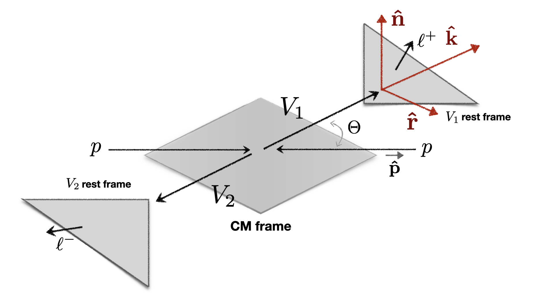
Figure 3.1: Unit vectors and momenta in the CM system [19], here specified for the weak gauge bosons production $p\,p\to V_{1}V_{2}$.

3.2   Polarization density matrices

3.2.1   Qubit polarization matrices: Spin-half fermions

The density matrix describing the polarization state $\lambda$ of a spin-half fermion $\psi_{\lambda}$ can be computed straightforwardly from the amplitude of the underlying production process

$$\mathcal{M}(\lambda)=\quantity[\bar{u}_{\lambda}\mathcal{A}],$$ (3.2)

with polarization $\lambda\in\{-\frac{1}{2},\frac{1}{2}\}$ along a given quantization direction. In the above formula we have indicated with $\mathcal{A}$ the term in the amplitude that multiplies the spinor $\bar{u}_{\lambda}$ of the produced fermion and we used square brackets to track the contractions of spinor indices.

The outgoing particle is then described by a state

$$\ket{\psi}=\sum_{\lambda}\mathcal{M}(\lambda)\ket{u_{\lambda}}$$ (3.3)

where $\ket{u_{\lambda}}$ is the Hilbert space representation of the spinor. The spinor-space density matrix is then obtained as

$$\tilde{\rho}_{\psi}=\frac{\outerproduct{\psi}{\psi}}{\innerproduct{\psi}{\psi}}=\frac{\sum_{\lambda\lambda^{\prime}}\quantity[\bar{u}_{\lambda}\mathcal{A}]\quantity[\bar{u}_{\lambda^{\prime}}\mathcal{A}]^{\dagger}\,\outerproduct{u_{\lambda}}{\bar{u}_{\lambda^{\prime}}}}{{\sum_{\lambda\lambda^{\prime}}\quantity[\bar{u}_{\lambda}\mathcal{A}]\quantity[\bar{u}_{\lambda^{\prime}}\mathcal{A}]^{\dagger}\,\innerproduct{\bar{u}_{\lambda^{\prime}}}{u_{\lambda}}}}.$$ (3.4)

By using the orthogonality relation $\innerproduct{\bar{u}_{\lambda^{\prime}}}{u_{\lambda}}\equiv\quantity[\bar{u}_{\lambda^{\prime}}u_{\lambda}]=2m\delta_{\lambda^{\prime}\lambda}$ the denominator can be rewritten as

$$\tilde{\rho}_{\psi}=\frac{\sum_{\lambda\lambda^{\prime}}\quantity[\bar{u}_{\lambda}\mathcal{A}]\quantity[\bar{u}_{\lambda^{\prime}}\mathcal{A}]^{\dagger}\,\outerproduct{u_{\lambda}}{\bar{u}_{\lambda^{\prime}}}}{2m{\sum_{\lambda}\quantity[\bar{u}_{\lambda}\mathcal{A}]\quantity[\bar{u}_{\lambda}\mathcal{A}]^{\dagger}}}=\frac{\sum_{\lambda\lambda^{\prime}}\quantity[\mathcal{A}\bar{u}_{\lambda^{\prime}}]^{\dagger}\quantity[\mathcal{A}\bar{u}_{\lambda}]\,\outerproduct{u_{\lambda}}{\bar{u}_{\lambda^{\prime}}}}{2m\,\absolutevalue{\mathcal{M}}^{2}}\,,$$ (3.5)

where $m$ is the mass of the fermion and $\absolutevalue{\mathcal{M}}^{2}$ is the squared amplitude for the production process summed over the spin.

To obtain the polarization density matrix we use the projection operators [126, 35]

$$\frac{\outerproduct{u_{\lambda}}{\bar{u}_{\lambda^{\prime}}}}{2m}=\frac{\Pi^{u}_{\lambda\lambda^{\prime}}}{2m}=\frac{1}{4m}\quantity(\not{p}+m)\quantity(\delta_{\lambda\lambda^{\prime}}+\gamma_{5}\sum_{i}\not{n}_{i}\sigma^{i}_{\lambda\lambda^{\prime}})$$ (3.6)

and

$$\frac{\outerproduct{v_{\lambda}}{\bar{v}_{\lambda^{\prime}}}}{2m}=\frac{\Pi^{v}_{\lambda\lambda^{\prime}}}{2m}=\frac{1}{4m}\quantity(\not{p}-m)\quantity(\delta_{\lambda\lambda^{\prime}}+\gamma_{5}\sum_{i}\not{n}_{i}\sigma^{i}_{\lambda\lambda^{\prime}})\,,$$ (3.7)

where $\sigma_{i}$ are the Pauli matrices and $\{n_{i}^{\mu}\}$ is a triad of space-like four-vectors, each satisfying $n_{i}^{\mu}p_{\mu}=0$, obtained by boosting the canonical basis of the spin four-vector $n$ to the frame where the fermion has four-momentum $p$. By means of the projector operators we then obtain

$$\rho_{\lambda\lambda^{\prime}}=\quantity[\frac{\Pi^{u}_{\lambda\lambda^{\prime}}}{2m}\tilde{\rho}_{\psi}]=\frac{\quantity[\mathcal{A}\mathcal{A}^{\dagger}\Pi^{u}_{\lambda\lambda^{\prime}}]}{\absolutevalue{\mathcal{M}}^{2}}\equiv\frac{1}{2}\left(\mathbb{1}+\sum_{i=1}^{3}s^{i}\sigma_{i}\right)_{\lambda\lambda^{\prime}}\,,$$ (3.9)

where $s^{i}$ are the components of the fermion polarization vector that generally depend on the kinematic variables of the underlying production process. The generalization to processes yielding more than one spin-half fermion in the final state is straightforward and the resulting density matrices can be decomposed on the basis of the tensor products of Pauli and unit matrices. For the case of two fermions, this yields the bipartite density matrix Eq. (2.38), the parameters of which are given in terms of expectation values in Eq. (2.39) and Eq. (2.40).

3.2.2   Qubit polarization matrices: Photons

The production of massless spin-1 particles (photons) is the other instance of a system whose polarizations are qubits. Let us consider the amplitude for the production of a photon with helicity $\lambda\in\{+1,-1\}$ and momentum $k$

$$\mathcal{M}(\lambda,k)=\mathcal{A}_{\mu}\varepsilon^{\mu*}_{\lambda}(k)$$ (3.10)

where $\mathcal{A}_{\mu}$ denotes the coefficient multiplying the (conjugated) polarization vector $\varepsilon^{\mu}_{\lambda}$ of the produced photon. In the following we will remove the momentum dependence in $\mathcal{M}$.

The polarization four-vectors $\varepsilon_{\lambda}^{\mu}$, $\lambda\in\{1,2\}$ obey the conditions $\varepsilon_{\lambda}\cdot\varepsilon_{\lambda^{\prime}}=-\delta_{\lambda\,\lambda^{\prime}}$, $\varepsilon_{\lambda}\cdot k=0$, where the contractions of Lorentz indices is left implied, and provide a basis for the linear polarizations. The polarization state $\ket{V^{\mu}}$ of the photon $V$ is consequently determined as

$$\ket{V^{\nu}}=\sum_{\lambda}\mathcal{M}(\lambda)\ket{\varepsilon^{\nu}_{\lambda}}\,,$$ (3.11)

where $\ket{\varepsilon^{\nu}_{\lambda}}$ is a representation of the polarization vector $\varepsilon^{\mu}_{\lambda}$ in the Hilbert space. The covariant density matrix describing the state is then obtained as

$$\tilde{\rho}^{\mu\nu}=-\frac{\outerproduct{V^{\mu}}{V^{\nu}}}{\innerproduct{V^{\mu}}{V_{\mu}}}$$ (3.12)

after the normalization of the state vector and having inserted a factor of $(-1)$ to account for the signature $(1,\,-1,\,-1,\,-1)$ of the Minkowski metric. The polarization density matrix $\rho_{\lambda\lambda^{\prime}}$ is then obtained by contracting the density matrix in Eq. (3.12) with the projector $\mathcal{P}^{\mu\nu}_{\lambda\lambda^{\prime}}(k)=\varepsilon^{\mu*}_{\lambda}(k)\,\varepsilon^{\nu}_{\lambda^{\prime}}(k)\,$ as

$$\rho_{\lambda\lambda^{\prime}}=\mathcal{P}^{\mu\nu}_{\lambda\lambda^{\prime}}\,\tilde{\rho}_{\mu\nu}.$$ (3.13)

From the orthonormality relation $\varepsilon_{\lambda}\cdot\varepsilon_{\lambda^{\prime}}=-\delta_{\lambda\,\lambda^{\prime}}$ and Eqs. (3.10)-(3.13) it follows that

$$\rho_{\lambda\lambda^{\prime}}=\frac{\mathcal{M}(\lambda)\mathcal{M}^{\dagger}(\lambda^{\prime})}{\sum_{\lambda^{\prime\prime}}\mathcal{M}^{\dagger}(\lambda^{\prime\prime})\mathcal{M}(\lambda^{\prime\prime})}=\frac{\mathcal{A}_{\mu}\mathcal{A}^{\dagger}_{\nu}\mathcal{P}^{\mu\nu}_{\lambda\lambda^{\prime}}}{\absolutevalue{\mathcal{M}}^{2}}.$$ (3.14)

The covariant density matrix in Eq. (3.12) can be decomposed in terms of the Stokes parameters $\xi^{i}$ [127] as:

$$\tilde{\rho}_{\mu\nu} =\frac{1}{2}\sum_{\lambda\lambda^{\prime}}\varepsilon^{\lambda}_{\mu}\Big{(}\mathbb{1}+\sum_{i=1}^{3}\xi^{i}\sigma_{i}\Big{)}_{\lambda\lambda^{\prime}}\varepsilon^{\lambda^{\prime}}_{\nu}$$

$$=\frac{1}{2}\Big{(}\varepsilon_{\mu}^{(1)}\varepsilon_{\nu}^{(1)}+\varepsilon_{\mu}^{(2)}\varepsilon_{\nu}^{(2)}\Big{)}+\frac{\xi_{1}}{2}\Big{(}\varepsilon_{\mu}^{(1)}\varepsilon_{\nu}^{(2)}+\varepsilon_{\mu}^{(2)}\varepsilon_{\nu}^{(1)}\Big{)}$$

$$\quad-\frac{i\xi_{2}}{2}\Big{(}\varepsilon_{\mu}^{(1)}\varepsilon_{\nu}^{(2)}-\varepsilon_{\mu}^{(2)}\varepsilon_{\nu}^{(1)}\Big{)}+\frac{\xi_{3}}{2}\Big{(}\varepsilon_{\mu}^{(1)}\varepsilon_{\nu}^{(1)}-\varepsilon_{\mu}^{(2)}\varepsilon_{\nu}^{(2)}\Big{)}\,.$$ (3.15)

In matrix form, the density matrix on the helicity basis in Eq. (3.14) is given by

$$\rho_{\lambda\lambda^{\prime}}=\frac{1}{2}\Big{(}\mathbb{1}+\sum_{i=1}^{3}\xi^{i}\sigma_{i}\Big{)}_{\lambda\lambda^{\prime}}$$ (3.16)

and the Stokes coefficients $\xi^{i}$ can be obtained by taking the traces, namely $\xi^{i}={\rm Tr}[\rho\sigma_{i}]$.

In the case of a two-photon system, the corresponding density matrix will depend on the Stokes parameters $\vec{\xi}^{(a)}$ and $\vec{\xi}^{(b)}$ of the photons $a$ and $b$. The generalization is straightforward and the resulting density matrix can be decomposed on the basis of the tensor products of Pauli and unit matrices as in Eq. (2.38).

3.2.3   X states

A great deal of simplification occurs if the matrix $C$, written on the basis of (3.1),

$$C=\begin{pmatrix}C_{nn}&C_{nr}&C_{nk}\\ C_{rn}&C_{rr}&C_{rk}\\ C_{kn}&C_{kr}&C_{kk}\end{pmatrix}\,,$$ (3.17)

only has a pair of non-vanishing off-diagonal terms, for instance $C_{kr}=C_{rk}$. The eigenvalues of $\mathfrak{m}_{12}$ are given in this case by

$$C_{nn}^{2},\quad\frac{1}{4}\Big{[}C_{kk}+C_{rr}+\sqrt{(C_{kk}^{2}-C_{rr})^{2}+4C_{kr}^{2}}\Big{]}^{2},\quad\frac{1}{4}\Big{[}C_{kk}+C_{rr}-\sqrt{(C_{kk}^{2}-C_{rr})^{2}+4C_{kr}^{2}}\Big{]}^{2}\,.$$ (3.18)

The result in Eq. (3.18) is an example of the simplification that occurs for a class of states, dubbed X states [128] because their density matrix takes the form

$$\rho_{X}=\begin{pmatrix}a&0&0&w\\ 0&b&z&0\\ 0&z^{*}&c&0\\ w^{*}&0&0&d\end{pmatrix}\,.$$ (3.19)

All matrices $C$ with only one non-vanishing coefficient off diagonal give rise to a density matrix that falls into this class.

The eigenvalues of the matrix $R$ in Eq. (2.21) in the case of $\rho_{X}$ can be readily written and the concurrence $\mathscr{C}[\rho]$ computed by means of a particularly simple formula; when $B_{i}^{\pm}=0$ and the only off-diagonal non-vanshing element of $C$ is $C_{rk}=C_{kr}$, one has

$$\mathscr{C}[\rho]=\frac{1}{2}\max\Big{[}0,\,|C_{rr}+C_{nn}|-(1+C_{kk})\,,\,\sqrt{(C_{rr}-C_{nn})^{2}+4C_{rk}^{2}}-|1-C_{kk}|\Big{]}\,.$$ (3.20)

3.2.4   Qutrit polarisation matrices

Massive spin-1 particles provide an instance of a system whose polarizations implement qutrits. Let us consider the amplitude for the production of a massive gauge boson with helicity $\lambda\in\{+1,0,-1\}$ and momentum $p$

$$\mathcal{M}(\lambda,p)=\mathcal{A}_{\mu}\varepsilon^{\mu*}_{\lambda}(p)$$ (3.21)

where $\mathcal{A}_{\mu}$ denotes the coefficient multiplying the (conjugated) polarization vector $\varepsilon^{\mu}_{\lambda}$ of the produced boson. The polarization state $\ket{V^{\mu}}$ of the boson $V$ is consequently determined as

$$\ket{V^{\nu}}=\sum_{\lambda}\mathcal{M}(\lambda)\ket{\varepsilon^{\nu}_{\lambda}}\,,$$ (3.22)

where $\ket{\varepsilon^{\nu}_{\lambda}}$ is a representation of the polarization vector in the Hilbert space. The covariant density matrix describing the state is then obtained as

$$\tilde{\rho}^{\mu\nu}=-\frac{\outerproduct{V^{\mu}}{V^{\nu}}}{\innerproduct{V^{\mu}}{V_{\mu}}}$$ (3.23)

after the normalization of the state vector and having inserted a factor of $(-1)$ to account for the signature $(1,\,-1,\,-1,\,-1)$ of the Minkowski metric $g_{\mu\nu}$. The polarization density matrix is then obtained through the projector $\mathcal{P}^{\mu\nu}_{\lambda\lambda^{\prime}}(p)=\varepsilon^{\mu*}_{\lambda}(p)\,\varepsilon^{\nu}_{\lambda^{\prime}}(p)\,$:

$$\rho_{\lambda\lambda^{\prime}}=\mathcal{P}^{\mu\nu}_{\lambda\lambda^{\prime}}\,\tilde{\rho}_{\mu\nu}.$$ (3.24)

From the orthonormality relation $g_{\mu\nu}\,\varepsilon^{\mu}_{\lambda}(p)\,\varepsilon^{\nu}_{\lambda^{\prime}}(p)=-\delta_{\lambda\lambda^{\prime}}$ and Eqs. (3.21)-(3.24) it follows that

$$\rho_{\lambda\lambda^{\prime}}=\frac{\mathcal{M}(\lambda)\mathcal{M}^{\dagger}(\lambda^{\prime})}{\sum_{\lambda^{\prime\prime}}\mathcal{M}^{\dagger}(\lambda^{\prime\prime})\mathcal{M}(\lambda^{\prime\prime})}=\frac{\mathcal{A}_{\mu}\mathcal{A}^{\dagger}_{\nu}\mathcal{P}^{\mu\nu}_{\lambda\lambda^{\prime}}}{\absolutevalue{\mathcal{M}}^{2}}.$$ (3.25)

In order to obtain an expression for the projector $\mathcal{P}$, consider the explicit form of the wave vector of a massive gauge boson with helicity $\lambda$

$$\varepsilon^{\mu}_{\lambda}(p)=-\frac{1}{\sqrt{2}}|\lambda|\left(\lambda\,n_{1}^{\mu}+i\,n_{2}^{\mu}\right)+\Big{(}1-|\lambda|\Big{)}n_{3}^{\mu},$$ (3.26)

where the four-vectors $n_{i}=n_{i}(p)$, $i\in\{1,2,3\}$, form a right-handed triad and are obtained by boosting the linear polarization vectors defined in the frame where the boson is at rest to a frame where it has momentum $p$. With the above expression one finds [129, 130, 131]

$$\mathcal{P}^{\mu\nu}_{\lambda\lambda^{\prime}}(p)=\frac{1}{3}\left(-g^{\mu\nu}+\frac{p^{\mu}p^{\nu}}{m_{V}^{2}}\right)\delta_{\lambda\lambda^{\prime}}-\frac{i}{2m_{V}}\epsilon^{\mu\nu\alpha\beta}p_{\alpha}n_{i\,\beta}\left(S_{i}\right)_{\lambda\lambda^{\prime}}-\frac{1}{2}n_{i}^{\mu}n_{j}^{\nu}\left(S_{ij}\right)_{\lambda\lambda^{\prime}},$$ (3.27)

where $m_{V}$ is the invariant mass of the vector boson $V$, $\epsilon^{\mu\nu\alpha\beta}$ the permutation symbol ($\epsilon^{0123}=1$) and $S_{i}$, $i\in\{1,2,3\}$, are the $SU(2)$ generators in the spin-1 representation—the eigenvectors of $S_{3}$, corresponding to the eigenvalues $\lambda\in\{+1,0,-1\}$, define the helicity basis. The spin matrix combinations appearing in the last term are given by

$$S_{ij}=S_{i}S_{j}+S_{j}S_{i}-\frac{4}{3}\mathbb{1}\,\delta_{ij},$$ (3.28)

with $i,j\in\{1,2,3\}$ and $\mathbb{1}$ being the $3\times 3$ unit matrix.

Eqs. (3.25) and (3.27) make it possible to compute the polarization density matrix for an ensemble of $V$ bosons produced in repeated reactions described by the amplitude $\mathcal{M}$. The formalism can be straightforwardly extended to processes yielding a bipartite qutrit state formed by two massive gauge bosons, $V_{1}$ and $V_{2}$. In this case we have

$$\rho=\frac{{\mathcal{A}}_{\mu\nu}{\mathcal{A}}^{\dagger}_{\mu^{\prime}\nu^{\prime}}}{\absolutevalue{\mathcal{M}}^{2}}\left(\mathcal{P}^{\mu\mu^{\prime}}(k_{1})\otimes\mathcal{P}^{\nu\nu^{\prime}}(k_{2})\right),$$ (3.29)

where $k_{1}$ and $k_{2}$ denote the momenta of the vector bosons in a given frame. The eight components of $f_{a}$ and $g_{a}$, as well as the 64 elements of $h_{ab}$, can be obtained by projecting the density matrix (2.61) on the desired subspace basis using the orthogonality relations, yielding

$$f_{a}=\frac{1}{6}\,\mbox{Tr}\,\left[\rho\left(T^{a}\otimes\mathbb{1}\right)\right]\,,~{}~{}g_{a}=\frac{1}{6}\,\mbox{Tr}\,\left[\rho\left(\mathbb{1}\otimes T^{a}\right)\right]\,,~{}~{}h_{ab}=\frac{1}{4}\,\mbox{Tr}\,\left[\rho\left(T^{a}\otimes T^{b}\right)\right]\,.$$ (3.30)

All the terms computed via Eq. (3.30) are Lorentz scalars.

3.3   Reconstructing density matrices from events

The preceding Section described how to calculate the probability of the directions of the emitted decay products based on the spin density matrix of the parent particle. The role of the experimentalist is to invert this process, and to determine the spin density matrix from the observable angular distributions. This inverse problem is possible provided that (i) the decays depend sufficiently on $\rho$ that the process is invertible in principle and (ii) that the daughter particle distribution functions (PDFs) can be determined in the rest-frame of the parent particles.

The simplest case of the two-body decay of a scalar state is uninteresting in this regard; the spin density matrix is the one-dimensional identity $\mathbb{1}_{1}$, and the angular distributions are isotropic.

3.3.1   Qubits

For the simplest non-trivial case, the decay of a spin-half particle, such as a top quark or antiquark, the density matrix Eq. (3.9) can be represented by the polarization vector $\vec{B}\equiv\langle\vec{s}\rangle$, where the average is taken over the distributions of the kinematic parameters that determine $\vec{s}$. The role of the projectors in Eq. (3.9) is to produce an angular dependence that the probability density function for the decay product lie into the infinitesimal solid angle close to $\vec{n}$:

$$p(\vec{n};\rho)=\frac{1}{4\pi}(1+\kappa\,{\vec{B}}\cdot\vec{n}).$$ (3.31)

The decay depends only on $\vec{B}$ and on the so-called ‘spin-analysing power’ $\kappa:-1\leq\kappa\leq 1$ of the daughter particle in the decay. Near-maximum values of $|\kappa|\approx 1.0$ are obtained for charged leptons emitted in top-quark decays [132].

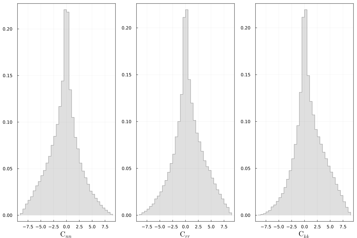
Figure 3.2: Example of distribution of the three diagonal elements of the matrix $C_{ij}$ The average (see Eq. (3.33)) and standard deviation of these histograms give the mean value and uncertainty of the corresponding coefficient. The events are taken from an (unpublished) simulation of the process $e^{+}e^{-}\to\tau^{+}\tau^{-}$ by two of the authors.

The process of measuring $\rho$ from data in this case is equivalent to determining the polarisation $\vec{B}$ from the angular distribution. This can be achieved by measurement of the angular distributions, except the (not infrequent) special case when $\kappa=0$ when the decay is isotropic and hence the process non-invertible. For $\kappa\neq 0$ the polarisation components are given by projecting out the polarisation components of Eq. (3.31) which can be achieved from the averages of the angular distributions of the polarimetric vector $\vec{n}$

$$B^{\pm}_{i}=\frac{3}{\kappa_{\pm}}\frac{1}{\sigma}\int\mbox{d}\Omega^{\pm}\frac{\mbox{d}\sigma}{\mbox{d}\Omega^{\pm}}(\vec{n}^{\pm}\cdot\hat{e}_{i}),$$ (3.32)

where $\{\hat{e}_{i}\}$, $i=1,2,3$, is an orthonormal basis—usually $\{{\bf\hat{n}},{\bf\hat{r}},{\bf\hat{k}}\}$. The correlation parameters $C_{ij}$ can also be determined by taking the average

$$C_{ij}=\frac{9}{\kappa_{+}\kappa_{-}}\frac{1}{\sigma}\int\mbox{d}\Omega^{+}\mbox{d}\Omega^{-}\frac{\mbox{d}\sigma}{\mbox{d}\Omega^{+}\mbox{d}\Omega^{-}}\,(\vec{n}^{+}\cdot\hat{e}_{i})(\vec{n}^{-}\cdot\hat{e}_{j})$$ (3.33)

weighted again by the differential cross section.

For the case of measuring the spin of $t\bar{t}$ systems from the resultant lepton angular distributions in their parents’ respective rest frames, the spin analysing powers in Eq. (3.33) are $\kappa_{+}=+1.0$ and $=\kappa_{-}=-1.0$ for the positive and negative leptons respectively. An example of these distributions obtained from Monte Carlo simulations can be found in Figure 3.2.

3.3.2   Qutrits

The spin 1 gauge bosons also act as their own polarimeters. For instance, in the decay $W^{+}\to\ell^{+}\nu_{\ell}$ the lepton $\ell^{+}$ is produced in the positive helicity state while the neutrino $\nu_{\ell}$ in the negative helicity state. The polarization of the $W^{+}$ is therefore measured to be $+1$ in the direction of the lepton $\ell^{+}$. The opposite holds for the decay $W^{-}\to\ell^{-}\bar{\nu}_{\ell}$ and the polarization of the $W^{-}$ is therefore measured to be $-1$ in the direction of the lepton $\ell^{-}$. In both the cases, the momenta of the final leptons (as in Fig. 3.1) provide a measurement of the gauge boson polarizations. The same is true for final jets from $d$ and $s$ quarks. These momenta are the only information that we need to extract from the numerical simulation or the actual data.

How do we go about reconstructing the correlation coefficients $h_{ab}$, $f_{a}$ and $g_{a}$ of the density matrix starting from the momenta of the final leptons? This problem has been recently discussed in [133], which we mostly follow in the remainder of this section.

The cross section we are interested in can be written as [134]

$$\frac{1}{\sigma}\frac{\mbox{d}\sigma}{\mbox{d}\Omega^{+}\,\mbox{d}\Omega^{-}}=\left(\frac{3}{4\pi}\right)^{2}\mbox{Tr}\,\Big{[}\rho_{V_{1}V_{2}}\left(\Pi_{+}\otimes\Pi_{-}\right)\Big{]}\,,$$ (3.34)

in which the angular volumes $\mbox{d}\Omega^{\pm}=\sin\theta^{\pm}\mbox{d}\theta^{\pm}\,\mbox{d}\phi^{\pm}$ are written in terms of the spherical coordinates (with independent polar axes) for the momenta of the final charged leptons in the respective rest frames of the decaying particles. The dependence on the invariant mass $m_{VV}$ and scattering angle $\Theta$ in Eq. (3.34) is implied. The density matrix $\rho_{V_{1}V_{2}}$ in Eq. (3.34) is that for the production of two gauge bosons given in Eq. (2.61).

The density matrices $\Pi_{\pm}$ describe the polarization of the decaying gauge bosons. The final leptons are taken to be massless—for their masses are negligible with respect to that of the gauge boson. They are projectors in the case of the $W$-bosons because of their chiral coupling to leptons. These matrices can be computed by rotating to an arbitrary polar axis the spin $\pm 1$ states of the weak gauge bosons taken in the $z$ direction and are given, in the Gell-Mann basis, as

$$\Pi_{\pm}=\frac{1}{3}\,\mathbb{1}+\frac{1}{2}\sum_{i=a}^{8}\mathfrak{q}^{a}_{\pm}\,T^{a}\,,$$ (3.35)

where the Wigner functions $\mathfrak{q}^{a}_{\pm}$ can be written in terms of the respective spherical coordinates, as reported in Eq. (B.5) of Appendix B.2, for the decay of $W$-bosons.

We can define another set of functions

$$\mathfrak{p}_{\pm}^{n}=\sum_{m}(\mathfrak{m}^{-1}_{\pm})_{m}^{n}\,\mathfrak{q}_{\pm}^{m}$$ (3.36)

orthogonal to those in Eq. (B.5):

$$\left(\dfrac{3}{4\,\pi}\right)\int\mathfrak{p}_{\pm}^{n}\,\mathfrak{q}_{\pm}^{m}\,\mbox{d}\Omega^{\pm}=2\,\delta^{nm}\,.$$ (3.37)

In Eq. (3.36), $\mathfrak{m}^{-1}$ is the inverse of the matrix

$$(\mathfrak{m}_{\pm})^{nm}=\left(\dfrac{3}{8\,\pi}\right)\int\mathfrak{q}_{\pm}^{n}\,\mathfrak{q}_{\pm}^{m}\,\mbox{d}\Omega^{\pm}\,,$$ (3.38)

which is assumed to exist. The explicit form of the functions $\mathfrak{p}_{\pm}^{n}$ are given in Appendix B.2 Eq. (B.6).

The functions in Eq. (3.36) can be used to extract the correlation coefficients $h_{ab}$ from the bi-differential cross section in Eq. (3.34) through the projection

$$h_{ab} = \frac{1}{4\,\sigma}\int\int\frac{\mbox{d}\sigma}{\mbox{d}\Omega^{+}\,\mbox{d}\Omega^{-}}\,\mathfrak{p}_{+}^{a}\,\mathfrak{p}_{-}^{b}\,\mbox{d}\Omega^{+}\mbox{d}\Omega^{-}\,.$$ (3.39)

The correlation coefficients $f_{a}$ and $g_{a}$ can be obtained in similar fashion by projecting the single differential cross sections:

$$f_{a} = \frac{1}{2\,\sigma}\int\frac{\mbox{d}\sigma}{\mbox{d}\Omega^{+}}\,\mathfrak{p}_{+}^{a}\,\mbox{d}\Omega^{+}\,,$$

$$g_{a} = \frac{1}{2\,\sigma}\int\frac{\mbox{d}\sigma}{\mbox{d}\Omega^{-}}\,\mathfrak{p}_{-}^{a}\,\mbox{d}\Omega^{-}\,.$$ (3.40)

The density matrices $\Pi_{\pm}$ are not projectors in the case of the $Z$-bosons because the coupling between $Z$-bosons and leptons in the Lagrangian,

$$-i\frac{g}{\cos\theta_{W}}\Big{[}g_{L}(1-\gamma^{5})\gamma_{\mu}+g_{R}(1+\gamma^{5})\gamma_{\mu}\Big{]}\,Z^{\mu}\ ,$$ (3.41)

contains both right- and left-handed components, whose strengths are controlled by the coefficients $g_{L}=-1/2+\sin^{2}\theta_{W}$ and $g_{R}=\sin^{2}\theta_{W}$. In this case, one must introduce a generalized form of the functions in Eq. (B.5) which is defined as the following linear combinations

$$\tilde{\mathfrak{q}}^{n}=\dfrac{1}{g_{R}^{2}+g_{L}^{2}}\Big{[}g_{R}^{2}\,\mathfrak{q}^{n}_{+}+g_{L}^{2}\,\mathfrak{q}_{-}^{n}\Big{]}\,,$$ (3.42)

and define from these the corresponding orthogonal functions $\tilde{\mathfrak{p}}^{n}$ to be used in Eq. (3.30). They are the same for both the $\pm$ coordinate sets and given by

$$\tilde{\mathfrak{p}}^{n}=\sum_{m}\mathfrak{a}^{n}_{m}\mathfrak{p}_{+}^{m}\,,$$ (3.43)

where the matrix $\mathfrak{a}^{n}_{m}$ is given in Eq. (B.7) in Appendix B.2. The Eqs. (3.39)–(3.40) can be used after replacing the functions $\mathfrak{p}_{\pm}^{m}$ with $\tilde{\mathfrak{p}}^{n}$. For the $ZZ$ case, since the final state is that of a pair of indistinguishable bosons one should also include a symmetry factor of 1/2 for the $f_{a}$ and $g_{a}$ coefficients and 1/4 for the $h_{ab}$ [133].

Eqs. (3.39)–(3.40) provide the means to reconstruct the correlation functions of the density matrix from the distribution of the lepton momenta and thus allow to infer the expectation values of the observables ${\cal I}_{3}$ and $\mathscr{C}_{2}$ from the data. In a numerical simulation, or working with actual events, one extracts from each single event the coefficient of the combinations of trigonometric functions indicated in Eq. (B.6) in B.2; that coefficient is the corresponding entry of the correlation matrix in Eqs. (3.39)–(3.40). Running this procedure over all events gives an average value and its standard deviation.

An example showing the corresponding parameters, after this averaging for the process $H\rightarrow WW^{(*)}\rightarrow\ell^{+}\nu\ell^{-}\bar{\nu}$, assuming that the parental rest frames can be determined is shown in Figure 3.3.

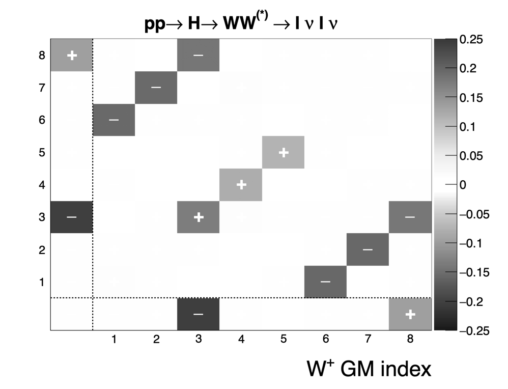
Figure 3.3: Reconstructed Gell-Mann parameters obtained from quantum state tomography of pairs of simulated $W^{\pm}$ bosons obtained from $H\rightarrow WW^{(*)}\rightarrow\ell^{+}\nu\ell^{-}\bar{\nu}$, (the bottom row of each plot contains the $B^{+}$ parameters for a $W^{+}$ boson, the leftmost column the $B^{-}$ parameters for the $W^{-}$ boson and the rows and columns 1-8 the $C_{ij}$ parameters. Bins are marked with “$+$” or “$-$” to indicate the sign of the reconstructed coefficient. The (0,0) element has no meaning. Adapted from [133] (CC BY 4.0).

3.3.3   Tensor representation for qutrits

The Gell-Mann representation of the density matrix Eq. (2.61) is only one possible parameterization. An alternative representation of the density matrix is in terms of tensor operator components, which for a single system can be written [135, 35, 134, 136, 137]

$$\rho=\frac{1}{2s+1}\sum_{L,M}(2L+1)(t_{M}^{L})^{*}T_{M}^{L}\,,$$ (3.44)

where $T^{L}_{M}$ are the matrices that represent the irreducible spherical tensor operators. We note that for the case of a qubit representation of the density matrix the Tensor representation and the Gell-Mann representation are identical, since both are provided by the standard Bloch vector, that is a parameterization based on the Pauli matrices.

For the general tensor representation, the orthogonality relationship

$$\mbox{Tr}\,{\left(T_{M^{\prime}}^{L^{\prime}}T_{M}^{L{\dagger}}\right)}=\frac{2s+1}{2L+1}\delta_{LL^{\prime}}\delta_{MM^{\prime}}$$ (3.45)

allows determination of the coefficients

$$t^{L}_{M}=\mbox{Tr}\,{\left(\rho T_{M}^{L}\right)}$$ (3.46)

from the observables. The procedure for extracting the coefficients from angular distributions in this framework is described in [137], which also includes discussion of the Wigner $\mathfrak{q}$ and $\mathfrak{p}$ functions for the irreducible tensors. The density matrices for bipartite systems can similarly be parameterized in terms of tensor products of tensor operators for the respective particles

$$\rho=\frac{1}{9}\Bigg{\{}\mathbb{1}\otimes\mathbb{1}+A^{1}_{LM}\left[T^{L}_{M}\otimes\mathbb{1}\right]+A^{2}_{LM}\left[\mathbb{1}\otimes T^{L}_{M}\right]+C_{L_{1}M_{1}L_{2}M_{2}}\left[T^{L_{1}}_{M_{1}}\otimes T^{L_{2}}_{M_{2}}\right]\Bigg{\}}\,.$$ (3.47)

The resultant angular distributions for $W^{\pm}$ boson decays, in terms of related parameters are given in [136]. The equivalent distributions for the $Z$ boson are provided in [138].

The analyses outlined in this Section can be experimentally challenging because both the CM frame of the collision and the rest frame of the parents must be determined in order to compute the various correlation coefficients with reasonable uncertainties. We discuss more details of the experimental aspects of these analyses in Section 4 for qubits and Section 5 for qutrits.

4   Qubits: top quarks, $\tau$ leptons and photons

Systems of two qubits, such as those arising from the polarizations of pairs of fermions (or photons), are routinely produced at the LHC and at SuperKEKB. We consider the production of top-quark pair $t\bar{t}$, $\tau$-lepton pair $\tau\bar{\tau}$ via the Drell-Yan mechanism and in the resonant Higgs boson decay $h\to\tau\bar{\tau}$ at the LHC, and in the $e^{+}e^{-}\to\tau\bar{\tau}$ at the Belle II experiment at SuperKEKB. We also include the di-photon system via the resonant Higgs decay process $h\to\gamma\gamma$, assuming (and it is a big assumption) that polarizations of the high-energy photons could be determined. For each of the considered processes, we provide the analytical predictions for the corresponding Bell inequality violation and quantum entanglement observables. Side by side with the analytical computation, it is crucial to have access to Monte Carlo simulations of the same processes in order to have an estimate of the uncertainty and therefore of the significance that can be reached for the values of the observables. The predictions, obtained by the reconstruction of the polarization density matrix by means of simulations of events, are provided, in dedicated sub-sections, for each of the considered processes.

4.1   Top-quark pair production at the LHC

At the parton level, the production of top-quark pair $t\bar{t}$ at the LHC receives two distinct contributions, namely from quark anti-quark ($q\bar{q}\to t\bar{t}$) and gluon-gluon annihilation ($gg\to t\bar{t}$) respectively. Corresponding Feynman diagrams in the SM are shown in Fig. 4.1. The analysis of the kinematics and polarizations is described for $q\bar{q}\to f\bar{f}$, where $f$ stands for a generic fermion in Appendix A.1. The same considerations on the kinematics and polarizations of the final states hold for the top-quark production via gluon-gluon fusion.

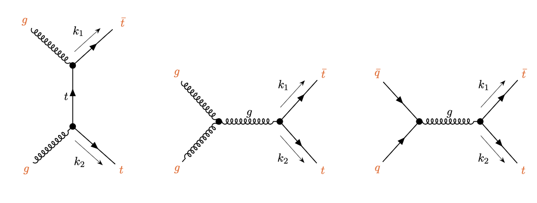
Figure 4.1: Feynman diagrams (at partonic tree-level) for top-antitop ($t\bar{t}$) production, for gluon ($gg$) and quark-pair ($q\bar{q}$) initial states.

The unpolarized differential cross section for the process

$$p+p\to t+\bar{t}\,.$$ (4.1)

is given in the basis Eq. (3.1) by [19, 66, 67]

$$\frac{\mbox{d}\sigma}{\mbox{d}\Omega\,\mbox{d}m_{t\bar{t}}}=\frac{\alpha_{s}^{2}\beta_{t}}{64\pi^{2}m_{t\bar{t}}^{2}}\Big{\{}L^{gg}(\tau)\,\tilde{A}^{gg}[m_{t\bar{t}},\,\Theta]+L^{qq}(\tau)\,\tilde{A}^{qq}[m_{t\bar{t}},\,\Theta]\Big{\}}\,,$$ (4.2)

where the combination of the two channels at partonic tree-level (see Fig. 4.1) $g+g\to t+\bar{t}$ and $q+\bar{q}\to t+\bar{t}$ in Eq. (4.2) is weighted by the respective parton luminosity functions $L^{gg,qq}(\tau)$

$$L^{gg}(\tau)=\frac{2\tau}{\sqrt{s}}\int_{\tau}^{1/\tau}\frac{\mbox{d}z}{z}q_{g}(\tau z)q_{g}\left(\frac{\tau}{z}\right)\quad\text{and}\quad L^{qq}(\tau)=\sum_{q=u,d,s}\frac{4\tau}{\sqrt{s}}\int_{\tau}^{1/\tau}\frac{\mbox{d}z}{z}q_{q}(\tau z)q_{\bar{q}}\left(\frac{\tau}{z}\right)\,,$$ (4.3)

where the functions $q_{j}(x)$ are the PDFs, $\alpha_{s}=g^{2}/4\pi$ and $\tau=m_{t\bar{t}}/\sqrt{s}$, with $m_{t\bar{t}}$ the invariant mass of the $t\bar{t}$ system. The explicit expressions for $\tilde{A}^{gg}$ and $\tilde{A}^{qq}$ are given in Appendix A.2. Their numerical values can be taken from, for instance, those provided by a recent sets (PDF4LHC21 [139]) for $\sqrt{s}=13$ TeV and factorization scale $q_{0}=m_{t\bar{t}}$.

The correlation coefficients $C_{ij}$ in the polarization density matrix for the $t\bar{t}$ pair production is given as [19, 66, 67]

$$C_{ij}[m_{t\bar{t}},\,\Theta]=\frac{L^{gg}(\tau)\,\tilde{C}_{ij}^{gg}[m_{t\bar{t}},\,\Theta]+L^{qq}(\tau)\,\tilde{C}_{ij}^{qq}[m_{t\bar{t}},\,\Theta]}{L^{gg}(\tau)\,\tilde{A}^{gg}[m_{t\bar{t}},\,\Theta]+L^{qq}(\tau)\,\tilde{A}^{qq}[m_{t\bar{t}},\,\Theta]}\,.\,$$ (4.4)

Notice that in the SM the polarization coefficients for the quark-pair $B_{i}^{qq}=0$ identically vanish.

The explicit expression for the coefficient $\tilde{C}_{ij}^{gg}$ and $\tilde{C}_{ij}^{qq}$ in Eq. (4.4) for the SM are collected in Appendix A.2. They are related to the corresponding correlation coefficients $C^{qq,gg}_{ij}$ for partonic processes by $\tilde{C}_{ij}^{gg}=C_{ij}^{gg}A^{gg}$ and $\tilde{C}_{ij}^{qq}=C_{ij}^{qq}A^{qq}$.

4.1.1   Entanglement in $t\bar{t}$ production

Top-quark pair production is the first process that has been considered in the current run of analyses. In [66] the expected entries of the density matrix were taken from [21] (in which they were computed for estimating classical correlations) and the concurrence computed.

The dependence of the entries of the polarization density matrix in Eq. (4.4) on the kinematic variables $\Theta$, the scattering angle, and $\beta_{t}=\sqrt{1-4m_{t}^{2}/m_{t\bar{t}}^{2}}$, is in general rather involved but it simplifies at $\Theta=\pi/2$ for which the top-quark pair is transversally produced and the entanglement is maximal. To understand the behaviour in this limit, one can choose the three vectors $\{{\bf\hat{n}},\,{\bf\hat{r}},\,{\bf\hat{k}}\}$ to point in the $\{\hat{x},\hat{y},\hat{z}\}$ directions and denote by $|0\rangle$ and $|1\rangle$ the eigenvectors of the Pauli matrix $\sigma_{z}$ with eigenvalues $-1$ and $+1$, respectively; similarly, let $|\small{-}\rangle$ and $|\small{+}\rangle$ be the analogous eigenvectors of $\sigma_{x}$ and $|\text{\small L}\rangle$ and $|\text{\small R}\rangle$ those of $\sigma_{y}$.

A set of quark pair spin density matrices that are relevant to this case are the projectors on pure, maximally entangled Bell states,

$$\rho^{(\pm)}=|\psi^{(\pm)}\rangle\langle\psi^{(\pm)}|\ ,\qquad|\psi^{(\pm)}\rangle=\frac{1}{\sqrt{2}}\big{(}|01\rangle\pm|10\rangle\big{)}\ ,$$ (4.5)

together with the mixed, unentangled states,

$$\rho^{(1)}_{\rm mix}=\frac{1}{2}\Big{(}|{\small++}\rangle\langle{\small++}|+|\small{--}\rangle\langle{\small--}|\Big{)}\ ,$$ (4.6)

$$\rho^{(2)}_{\rm mix}=\frac{1}{2}\Big{(}|\text{\small LR}\rangle\langle\text{\small LR}|+|\text{\small RL}\rangle\langle\text{\small RL}|\Big{)}\ ,$$ (4.7)

$$\rho^{(3)}_{\rm mix}=\frac{1}{2}\Big{(}|01\rangle\langle 01|+|10\rangle\langle 10|\Big{)}\ .$$ (4.8)

Let us treat separately the quark-antiquark $q\bar{q}$ and gluon-gluon $gg$ production channels. For the $q\bar{q}$ production channel, using the explicit expression collected in Appendix A.2 for the correlation coefficients $C_{ij}$, one obtains that the $t\bar{t}$ spin density matrix can be expressed as the following convex combination [140] :

$$\rho_{t\bar{t}}^{(q\bar{q})}=\lambda\rho^{(+)}+(1-\lambda)\rho^{(1)}_{\rm mix}\ ,\quad\text{with}\quad\lambda=\frac{\beta_{t}^{2}}{2-\beta_{t}^{2}}\in[0,1]\ ,$$ (4.9)

so that at high transverse momentum, for $\beta_{t}\rightarrow 1$, the spins of the $t\bar{t}$ pair tend to be generated in a maximally entangled state; this quantum correlation is however progressively diluted for $\beta_{t}<1$, vanishing at threshold, $\beta_{t}=0$, as the two spin state becomes a totally mixed, separable state.

The situation is different for the $gg$ production channel, as both at threshold and at high momentum the $t\bar{t}$ spins result maximally entangled, with $\rho_{t\bar{t}}^{(gg)}=\rho^{(+)}$ for $\beta_{t}\rightarrow 1$ and $\rho_{t\bar{t}}^{(gg)}=\rho^{(-)}$ when $\beta_{t}=\,0$. For intermediate values of $\beta_{t}$, the situation becomes more involved, and the two-spin density matrix can be expressed as the following convex combination:

$$\rho_{t\bar{t}}^{(gg)}=a\rho^{(+)}+b\rho^{(-)}+c\rho^{(1)}_{\rm mix}+d\rho^{(2)}_{\rm mix}\ ,$$ (4.10)

with non-negative coefficients [140]

$$a=\frac{\beta_{t}^{4}}{1+2\beta_{t}^{2}-2\beta_{t}^{4}}\ ,\quad b=\frac{(1-\beta_{t}^{2})^{2}}{1+2\beta_{t}^{2}-2\beta_{t}^{4}}\ ,\quad c=d=\frac{2\beta_{t}^{2}\big{(}1-\beta_{t}^{2}\big{)}}{1+2\beta_{t}^{2}-2\beta_{t}^{4}}\ ,\quad$$ (4.11)

so that $a+b+c+d=1$, while entanglement is less than maximal.

Including both the $q\bar{q}$- and $gg$-contributions leads to more mixing and therefore in general to additional loss of quantum correlations.

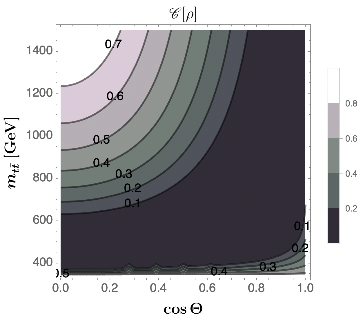
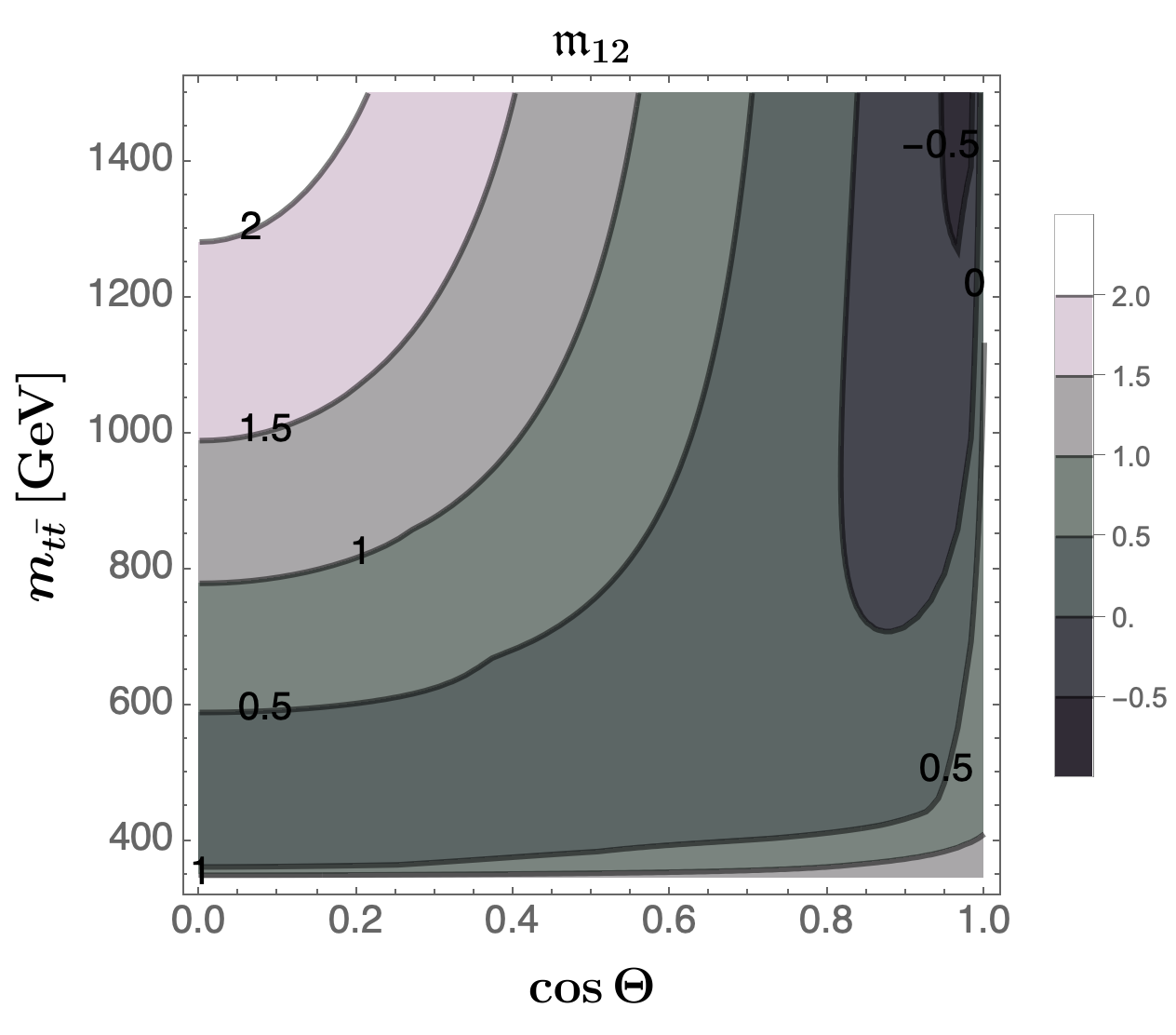
Figure 4.2: The observables $\mathscr{C}[\rho]$ (contour plot on the left) and $\mathfrak{m}_{12}$ (contour plot on the right) for $t\bar{t}$ production as functions of the kinematic variables $\Theta$ and $m_{t\bar{t}}$ across the entire available space (they are symmetric for $\cos\Theta<0$). Figures revised from [140] (CC BY 4.0).

All these features are manifest in the plot on the left-side in Fig. 4.2. There are two regions where entanglement is significant: in a sliver near threshold and for boosted tops for scattering angles close to $\pi/2$.

The strong dependence of the entanglement on the kinematic variables was first shown in [66]. That paper calculated the quantity

$$D=\frac{1}{3}\,\mbox{Tr}\,C_{ij}$$ (4.12)

and showed that close to threshold it is expected to be smaller than $-1/3$. This is a sufficient condition for entanglement, as $D$ is directly connected to concurrence by the relation $\mathscr{C}[\rho]=\max[-1-3D,\,0]/2$ [66].

The ATLAS Collaboration, applying the method proposed in [66], has recently [70] analyzed the $pp$ data and extracted the value of $D$ from the differential cross section

$$\frac{1}{\sigma}\frac{\mbox{d}\sigma}{\mbox{d}\cos\phi}=\frac{1}{2}\Big{(}1-D\cos\phi\Big{)}\,,$$ (4.13)

where $\phi$ is the angle between the respective leptons as computed in the rest frame of the decaying top and anti-top.

The analysis selected fully leptonic top pair events with one electron and one muon of opposite signs, and measured $D$ at the particle level in the near-threshold region $340\,{\rm GeV}<m_{t\bar{t}}<380$ GeV. After calibrating for detector acceptance and efficiency they measured [70]

$$D=-0.547\pm 0.002\;[{\rm stat.}]\pm 0.021\;[{\rm syst.}]\,.$$ (4.14)

This value is smaller than $-1/3$ with a significance of more than $5\sigma$, thus provides the first experimental observation of the presence of entanglement between the spins of the top quarks.

The observed entanglement is larger than that predicted by the simulations, suggesting that the simulations might require improved modelling of near-threshold effects in $t\bar{t}$ production.

4.1.2   Bell inequalities

The violation of the Bell inequality, coming from the entanglement of the top-quark pair, can be measured [67] by means of the Horodecki condition (2.47)

$$\mathfrak{m}_{12}\equiv m_{1}+m_{2}>1$$ (4.15)

as defined in Section 2.3. The values of the observable $\mathfrak{m}_{12}$ across the entire kinematic space available are shown on the right-hand side of Fig. 4.2.

Fig. 4.2 shows how the quantum entanglement as well as Bell inequality violation, encoded in the observable $\mathfrak{m}_{12}[C]$, increases as we consider larger scattering angles and $m_{t\bar{t}}$ masses. As expected from the qualitative discussion in the previous Section, the kinematic window where the observable $\mathfrak{m}_{12}$ is larger is for $m_{t\bar{t}}>900$ GeV and $\cos\Theta/\pi<0.2$. The mean value of $\mathfrak{m}_{12}$ in this bin is found to be 1.44 [140].

4.1.3   Monte Carlo simulations of events

A number of MC simulations have been performed of quantum observables in top-quark pair production. They consider fully- as well as semi-leptonic decays, and all agree with the analytic results. In addition, they provide an estimate of the uncertainty in both the amount of entanglement and of violation of Bell inequality. All works predict entanglement to be measurable at the LHC while they differ about the possibility of having a significant violation of Bell inequality. This process is now under scrutiny by the experimental Collaborations.

In [67], the process

$$p+p\to t+\bar{t}\to\ell^{\pm}\ell^{\mp}+\text{jets}+E^{\rm miss}_{\rm T}$$ (4.16)

is simulated by means of MadGraph5_aMC@NLO [141] at leading order at parton level and then hadronised and showered using Phytia8 [142]; the detector reconstruction is simulated within the Delphes [143] framework using the ATLAS detector card.

The operators related to entanglement and Bell inequality violation are computed from the simulated events by looking at the angular correlations of the pairs of charged leptons, as represented by the product of the cosines $\cos\theta^{i}_{+}$ and $\cos\theta^{j}_{-}$ as in Eq. (3.32). The matrix $C_{ij}$ is reconstructed from these by going to the rest frame of the top quark (which requires the reconstruction of the neutrino momenta).

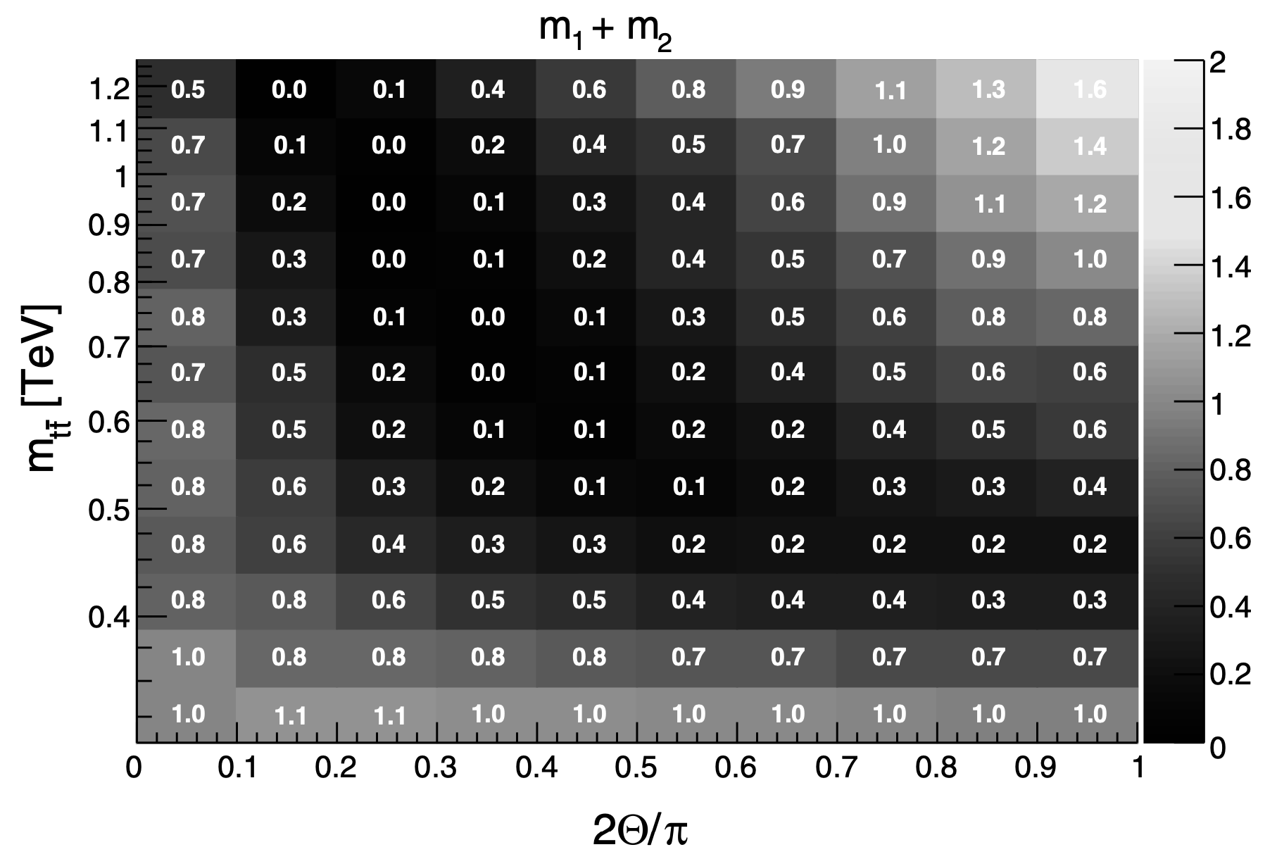
Figure 4.3: Simulation of the values of $\mathfrak{m}_{12}$ (here indicated as $m_{1}+m_{2}$) for the top-quark pair production at the LHC in bins, as a function of the invariant mass and the scattering angle. Values greater than 1 indicate violation of Bell inequality. Figure revisited from [67] (CC BY 4.0)

In [67], the authors concentrate on the region of high invariant mass and large scattering angles and estimate the value of $\mathfrak{m}_{12}$, after correcting for the bias. They predict that the violation can have a significance of $3\sigma$ for the combined Run 1 plus Run 2 at the LHC (with 300 fb^-1 of luminosity) and $4\sigma$ at the high-luminosity (Hi-Lumi) LHC (with 3 ab^-1 of luminosity). A smaller significance is found in [144] for the same kinematic region: below $1\sigma$ at Run 1 plus Run 2 and only 1.8$\sigma$ at the Hi-Lumi LHC. The difference seems to come from a different treatment of the uncertainties in going from the parton level (where the two analyses agree) to the unfolded events. The neutrino weighting technique [145] is used in [67] while RooUnfold framework [146] in [144].

How to enhance the violation of Bell inequality was discussed in [147] for the threshold region and more generally in [148].

In [149] and [150] the simulation is extended to include the semi-leptonic decays:

$$p+p\to t+\bar{t}\to\ell\nu+2b+2j\,.$$ (4.17)

The semi-leptonic channel contains more events, and fewer undetected particles, and could therefore provide a result with less uncertainty than the fully leptonic one. The same software packages, as described above, are used in the numerical simulations. The result is that tagging through the semi-leptonic channel brings more events even though the efficiency is reduced. An increase of a factor 1.6 in significance is expected between the fully leptonic and the semi-leptonic channels.

The combinations, derived from the CSHC inequality in Eq. (2.37),

$$|C_{rr}-C_{nn}|-\sqrt{2}>0\quad\text{or}\quad|C_{kk}+C_{rr}|>0$$ (4.18)

are used to mark the violation of the Bell inequality. Both works find a significance of $4\sigma$ at Hi-Lumi (with 3 ab^-1 of luminosity) for the violation of the Bell inequality in the region of large invariant mass and scattering angle.

One would expect the experimental Collaborations eventually to use both the semi- and leptonic channels in the analysis of the actual data.

4.2   $\tau$-lepton pair production at the LHC and SuperKEKB

The study of entanglement in $\tau$-lepton pairs was first proposed for $e^{+}e^{-}$ collisions at LEP [50]. It was extended in [140] for the production at the LHC and in [151] for that at SuperKEKB.

The procedure for computing the polarization density matrix for this process at the LHC follows the same steps as for the top quarks analyzed in Section 4.1, except for the main production mechanism. The dominant process in this case is the Drell-Yan production in which the quarks go into the $s$-channel either via a photon or a $Z$-boson which, in turn, decay into the $\tau$-lepton pair. The corresponding tree-level relevant Feynman diagrams for the $\tau$-pair production are shown in Fig.4.4.

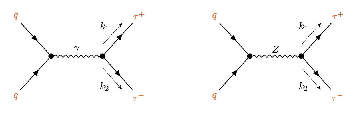
Figure 4.4: Feynman diagrams for $\tau^{-}\tau^{+}$ production via Drell-Yan mechanism at hadron collider.

In addition to the Drell-Yan mechanism production, in this case we also have the process in which the $\tau$ leptons originate from the resonant Higgs boson decay channel. We discuss the possible role of quantum entanglement in both of the processes, leaving the second mechanism to Section 4.3, which is devoted to the qubits systems arising from the Higgs boson decay.

The production process of $\tau$-lepton pairs via Drell-Yan mechanism in the SM receives contributions from the diagrams mediated by the $s$-channel photon, the $Z$-boson and their interference. These contributions provide an ideal laboratory for studying quantum entanglement among the qubits pairs of $\tau$-lepton pairs. Due to the fact that the fewer the contributions, the larger the entanglement (as mixing among quantum states suppresses quantum correlations), we expect this to be larger at low-energies (where the photon diagram dominates) or around the $Z$-boson pole (where the $Z$-boson diagram dominates). At low energies, the cross section is dominated by the photon term which produces entangled $\tau$-lepton pairs, while at high-energies all terms contribute and entanglement is suppressed. Around the $Z$-boson pole the cross section is dominated by the corresponding term with maximal entanglement.

The entries of the correlation matrix $C_{ij}$ from the process

$$p+p\to\tau^{-}+\tau^{+}\,.$$ (4.19)

are collected in Appendix A.3.

The two channels (with different initial quarks) are combined by weighting the respective contributions through the parton luminosity functions $L^{qq}(\tau)$ defined in Eq. (4.3). The corresponding unpolarized cross section is given by [140]

$$\frac{\mbox{d}\sigma}{\mbox{d}\Omega\,\mbox{d}m_{\tau\bar{\tau}}}=\frac{\alpha^{2}\beta_{\tau}}{64\pi^{2}m_{\tau\bar{\tau}}^{2}}\Big{\{}L^{uu}(\tau)\,\tilde{A}^{uu}[m_{\tau\bar{\tau}},\,\Theta]+\big{[}L^{dd}(\tau)+L^{ss}(\tau)\big{]}\,\tilde{A}^{dd}[m_{\tau\bar{\tau}},\,\Theta]\Big{\}}$$ (4.20)

where $\tau=m_{\tau^{-}\tau^{+}}/\sqrt{s}$ and $\alpha=e^{2}/4\pi$. For the numerical values of $L^{qq}(\tau)$, we can use those provided by PDF4LHC21 [139] for $\sqrt{s}=13$ TeV, as for the top pair before, but with factorization scale $q_{0}=m_{\tau\bar{\tau}}$. The explicit expressions for $\tilde{A}^{uu,dd}(m_{\tau\bar{\tau}})$ are given in Appendix A.3.

The full correlation matrix $C_{ij}$ is obtained by putting together all relevant contributions from the various $q\bar{q}$-production channels, weighted by suitable luminosity functions and with appropriate normalization. This effect leads to further mixing and in general to additional loss of entanglement.

For the correlation coefficients $C_{ij}$ we have [140]

$$C_{ij}[m_{t\bar{t}},\,\Theta]=\frac{L^{uu}(\tau)\,\tilde{C}_{ij}^{uu}[m_{\tau\bar{\tau}},\,\Theta]+\big{[}L^{dd}(\tau)+L^{ss}(\tau)\big{]}\,\tilde{C}_{ij}^{dd}[m_{\tau\bar{\tau}},\,\Theta]}{L^{uu}(\tau)\,\tilde{A}^{uu}[m_{\tau\bar{\tau}},\,\Theta]+\big{[}L^{dd}(\tau)+L^{ss}(\tau)\big{]}\,\tilde{A}^{dd}[m_{\tau\bar{\tau}},\,\Theta]}\,,$$ (4.21)

where the down-quark luminosity functions can be grouped together because they multiply the same correlation functions.

A much simpler formula holds at lepton colliders for the process

$$e^{+}+e^{-}\to\tau^{-}+\tau^{+}\,.$$ (4.22)

because there are no PDF luminosity functions, only one diagram and the CM energy is fixed at $\sqrt{s}=10$ GeV at SuperKEKB. This process was studied at SuperKEK in [151] to show how promising this setting can be for a study of Bell inequality violation. The expected concurrence is given in this case by a closed formula [151]:

$$\mathscr{C}[\rho]=\frac{\left(s-4\,m_{\tau}^{2}\right)\sin^{2}\Theta}{4\,m_{\tau}^{2}\sin^{2}\Theta+s\left(\cos^{2}\Theta+1\right)}\,.$$ (4.23)

4.2.1   Entanglement in $\tau\bar{\tau}$ production

The two spin-1/2 state of the $\tau$ pairs can be expressed by a density matrix having a general form as in Eq. (2.38), whose entries depend on the kinematic variable $\beta_{\tau}=\sqrt{1-4m_{\tau}^{2}/m_{\tau\bar{\tau}}^{2}}$, with $m_{\tau\bar{\tau}}$ the $\tau$-pair invariant mass, and on the scattering angle $\Theta$ in the $\tau\bar{\tau}$ CM frame.

Following the same notation and reference frame adopted for the top-pair production in Section 4.1, and focusing on the configuration of transversally produced lepton pairs ($\Theta=\pi/2$), we can distinguish three kinematic regions according to the following energy ranges: the low-energy one, at $m_{\tau\bar{\tau}}\ll m_{Z}$, where photon exchange dominates, the intermediate one at $m_{\tau\bar{\tau}}\simeq m_{Z}$, which is dominated by the $Z$ exchange, and finally the high-energy one, $m_{\tau\bar{\tau}}\gg m_{Z}$.

In the low-energy regime ($m_{\tau\bar{\tau}}\ll m_{Z}$), by using the results provided in the Appendix A.3 for the polarization and correlation coefficients of the density matrix in the $\tau$-pair case, we can see that the $\tau$-pair spin state can be represented by the convex combination as in (4.9) for the top-pair [140],

$$\rho_{\tau\bar{\tau}}=\lambda\rho^{(+)}+(1-\lambda)\,\rho^{(1)}_{\rm mix}\quad\text{with}\quad\lambda=\frac{\beta_{\tau}^{2}}{2-\beta_{\tau}^{2}}\in[0,1]\,;$$ (4.24)

at threshold, $\beta_{\tau}\simeq 0$, the quantum state is a totally mixed one, with no quantum correlations, while as $\beta_{\tau}\rightarrow 1$, the spins of the $\tau$-lepton pair tend to be generated in a maximally entangled state.

In the intermediate energy region, where the $Z$-channel starts to become relevant, this entanglement begins to loose coherence due to the increasing contribution of the interference term between the photon and $Z$ diagrams. Nevertheless, a revival of entanglement reappears as the $m_{\tau\bar{\tau}}$ approaches the resonant $Z$-channel region. In this region, using the notation and conventions introduced in the Appendix A.3, the two-spin density matrix can be described by the following convex combination, for all quark production channels :

$$\rho_{\tau\bar{\tau}}=\lambda\tilde{\rho}^{(+)}+(1-\lambda)\tilde{\rho}^{(2)}_{\rm mix}\ ,\qquad\lambda=\frac{(g_{A}^{\tau})^{2}-(g_{V}^{\tau})^{2}}{(g_{A}^{\tau})^{2}+(g_{V}^{\tau})^{2}}\ ,$$ (4.25)

where,

$$\tilde{\rho}^{(2)}_{\rm mix}=\frac{1}{2}\Big{(}|\text{\small RR}\rangle\langle\text{\small RR}|+|\text{\small LL}\rangle\langle\text{\small LL}|\Big{)}\ .\\$$ (4.26)

while

$$\tilde{\rho}^{(+)}=|\tilde{\psi}^{(+)}\rangle\langle\tilde{\psi}^{(+)}|\ ,\qquad|\tilde{\psi}^{(+)}\rangle=\frac{1}{\sqrt{2}}\Big{(}|\small{+-}\rangle+|\small{-+}\rangle\Big{)}\ ,$$ (4.27)

is a projector on a Bell state as in (4.5), expressed in terms of the eigenvectors of $\sigma_{x}$. Then, we could see that when $\lambda\to 1$, the density matrix $\rho_{\tau\bar{\tau}}$ in Eq. (4.25) turns out to be very close to the maximally entangled state $\tilde{\rho}^{(+)}$.

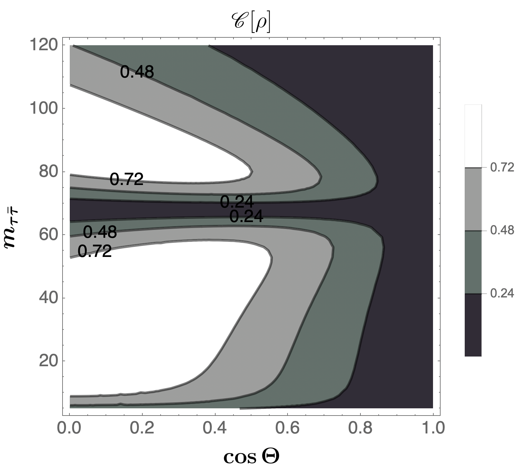
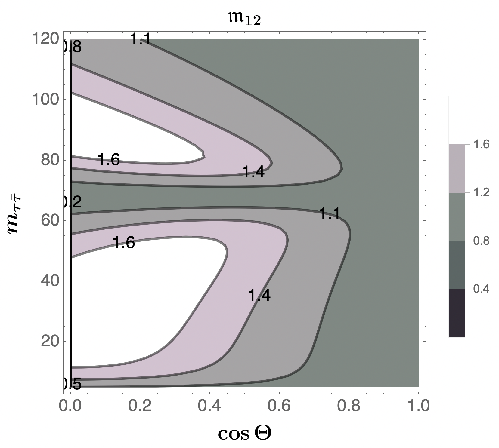
Figure 4.5: Concurrence and $\mathfrak{m}_{12}$ for the $\tau\bar{\tau}$ pair production at the LHC, as a function of the kinematic variables $\Theta$ and $m_{\tau\bar{\tau}}$ across the entire available space. Figures revisited from [140] (CC BY 4.0).

Finally, in the high energy regime ($m_{\tau\bar{\tau}}\gg m_{Z}$) both photon and $Z$ channel contribute, and, due to their mixing, a rapid depletion of entanglement is induced. In particular, for each $q\bar{q}$ production channel, the $\tau$-pair spin correlations can be described in terms of the following density matrix [140] :

$$\rho_{\tau\bar{\tau}}=\lambda^{q}\rho^{(+)}+(1-\lambda^{q})\tilde{\rho}^{(2)}_{\rm mix}\ ,\qquad\lambda^{q}=\frac{1-R_{-}^{q}}{1+R_{+}^{q}}\ ,$$ (4.28)

where $\rho^{(+)}$ is as in (4.5), while

$$R^{q}_{\pm}=\frac{\chi^{2}(m_{\tau\bar{\tau}}^{2})\big{[}(g_{A}^{q})+(g_{V}^{q})\big{]}\big{[}(g_{A}^{\tau})\pm(g_{V}^{\tau})\big{]}}{(Q^{q})^{2}(Q^{\tau})^{2}+2\,{\rm Re}\chi(m_{\tau\bar{\tau}}^{2})\,Q^{q}Q^{\tau}\,g_{V}^{q}g_{V}^{\tau}}\ .$$ (4.29)

Namely, in the case of the $u$ quark production channel, we have $\lambda^{u}\simeq 0.7$, so that some entanglement is preserved. On the other hand, for the $d$ quark production channel, since $\lambda^{d}\simeq 0.1$, the entanglement is essentially lost.

For completeness, it should be noticed that each $\tau$ lepton is produced in a partially polarized state, as some of the single-spin polarization coefficient $B_{i}^{\pm}$ in the spin density matrix are non-vanishing (see Appendix A.3). This is particularly relevant for the quark $d$ production channel, where the magnitude of these single particle terms is of the same order of the entries of the correlation matrix $C_{ij}$, while for the $u$ production channel they are about one order of magnitude smaller. This implies that the full density matrix describing the $\tau$-pair spin state $\rho_{\tau\bar{\tau}}$ is really in this case a mixture of (4.28) with additional states further reducing in general its entanglement content.

4.2.2   Bell inequalities

The same method presented in Section 4.1.2 for the top-quark pairs can be followed here. The values of the observable $\mathfrak{m}_{12}$, are shown in Fig. 4.5 across the entire kinematic space [140] for the hadron collider. These results confirms the qualitative analysis of entanglement in Section 4.2.1: Entanglement is close to maximal (that is, $\mathfrak{m}_{12}$ close to 2) for large scattering angles whenever the invariant mass of the $\tau$-lepton pairs selects one of the two possible channels with either the photon or the $Z$-boson exchange dominating.

The authors of [140] take the kinematic window where the $\tau$-lepton pair invariant mass is in the range $20{\rm GeV}<m_{\tau\bar{\tau}}<45{\rm GeV}$ and $|\cos\Theta|<0.2$ as the most favorable to test the Bell inequalities and there estimate the mean value of $\mathfrak{m}_{12}$ to be 1.88.

For the process at SuperKEKB, a simple analytic formula can be computed [151]:

$$\mathfrak{m}_{12}{}=1+\left(\frac{\left(s-4\,m_{\tau}^{2}\right)\sin^{2}\Theta}{4\,m_{\tau}^{2}\sin^{2}\Theta+s\left(\cos^{2}\Theta+1\right)}\right)^{2}\,,$$ (4.30)

The maximum value for both $\mathscr{C}[\rho]$ and $\mathfrak{m}_{12}{}$ are reached for scattering angles close to $\pi/2$, as shown in Fig. 4.6.

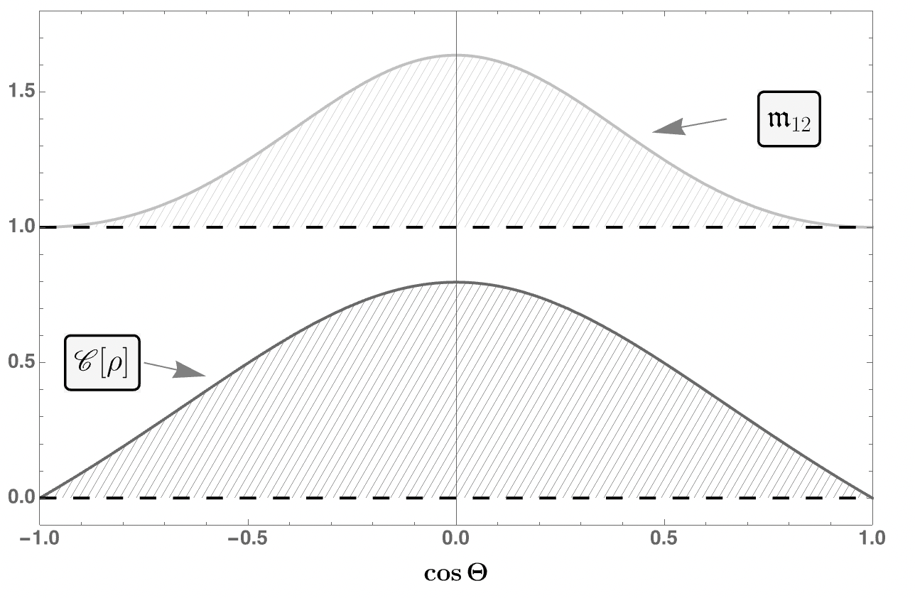
Figure 4.6: Concurrence and $\mathfrak{m}_{12}$ for $\tau\bar{\tau}$ pair production at SuperKEK. Figure revisited from [151] (CC BY 4.0).

4.2.3   Monte Carlo simulations of events

The production of $\tau\bar{\tau}$ pairs at SuperKEK appears very promising for the study of entanglement and Bell inequality violation because of the large number of events that are, in addition, very clean.

The polarization of the $\tau$-leptons can be extracted from the distribution in momenta of the final charged hadrons in the three decay channels: $\tau^{-}\to\pi^{-}\nu_{\tau}$, $\tau^{-}\to\pi^{-}\pi^{0}\nu_{\tau}$, and $\tau^{-}\to\pi^{-}\pi^{+}\pi^{-}\nu_{\tau}$. The combination of these decay channels covers about $21\%$ of $\tau$ pair decays.

In [151], a sample of $200$ million $e^{+}e^{-}\to\tau^{+}\tau^{-}$ Monte Carlo events was generated with the program MadGraph5_aMC@NLO [141], using leading-order matrix elements. The program PYTHIA [142] was used for the modeling of parton showers, hadronization processes, and $\tau$ decays. All the $\tau$ decay channels discussed above are included in the simulation. The events are analyzed on Monte Carlo truth level and after taking realistic experimental resolutions into account.

Both entanglement and Bell inequality violation are predicted to be observables with a significance well in excess of $5\sigma$.

4.3   Higgs boson decays in $\tau$-lepton pairs and two photons

The decay of the Higgs boson into a pair of fermions or two photons (see, Fig. 4.7), provides a physical process very similar to those utilized in atomic physics for studying entanglement. Because the final states originate from the decay a scalar particle, a pure state should be created. In this Section we discuss first the qubits system provided by the Higgs boson decay into $\tau$-lepton pair, then the decay into two photons. In this last case, we assume it will be possible in the future to determine the polarization of the photon.

Figure 4.7: Feynman diagrams for the Higgs boson $h$ decay into two $\tau$-leptons (left) and into two photons (right).

4.3.1   Entanglement and Bell inequalities in $h\to\tau\bar{\tau}$

The SM interaction Lagrangian for the decay of the Higgs boson into a pair of $\tau$ leptons is given by

$${\cal L}_{\text{\tiny SM}}=\frac{m_{\tau}}{v}\bar{\tau}\tau\,h\,,$$ (4.31)

where $v$ is the vacuum expectation value of the Higgs field $h$. On the basis of this interaction term, the elements of the matrix $C_{ij}$ entering the tau lepton-pair spin density matrix can be easily computed and is given by [140]

$$C=\begin{pmatrix}1&0&0\\ 0&1&0\\ 0&0&-1\end{pmatrix}\,,$$ (4.32)

where the $C$ matrix above is defined on the $\{\hat{n},\hat{r},\hat{k}\}$ spin basis as in Eq. (3.17). The entanglement ${\cal C}[\rho]$ is maximal and equal to 1. The sum of the square of the two largest eigenvalues gives $\mathfrak{m}_{12}=2$, so that the Bell inequality (2.36) is predicted to be maximally violated.

4.3.2   Monte Carlo simulations of events

The decay of the Higgs boson into $\tau$-lepton pairs has been analyzed in [152] and [153]. Both studies investigate $HZ$ associated production at future $e^{+}e^{-}$ colliders; the process would be difficult to reconstruct experimentally in the resonant production of the Higgs boson in the $s$-channel production in hadron colliders.

The Monte Carlo simulations are performed by means of MadGraph5_aMC@NLO [141], using leading-order matrix elements. The package TauDecay [154] is used for modeling the $\tau$ decays. Only the decays into a single pion are included. The momenta of the $\tau$-leptons are reconstructed by solving the kinematic equations holding for the (unknown) neutrino momenta. The kinematic reconstruction is possible up to a two-fold degeneracy.

In [152] it is found that one expects entanglement to be tested above 5$\sigma$ at both the International Linear Collider (ILC) and the Future Circular Collider (FCC-ee). The violation of Bell inequality is not expected to be observed at the ILC but it expected at the FCC-ee with a significance of about 3$\sigma$. It is found in [153] that the predicted significance is around $1\sigma$ for the Circular Electron Positron Collider (CEPC).

4.3.3   Entanglement and Bell inequalities in $h\to\gamma\gamma$

The entanglement of a system of two photon has been discussed in [155] and, more recently, in [140]. This system closely resembles those in atomic physics, in which the polarization of photons originating in atomic transitions are discussed.

The Higgs boson $h$ decays into two photons

$$h\to\gamma(k_{1})\,\gamma(k_{2})\,,$$ (4.33)

proceeds via an effective coupling $g_{\gamma\gamma h}$ provided in the SM by loop contributions. The effective Lagrangian in this case is given by

$${\cal L}=-\frac{1}{4}\,g_{\gamma\gamma h}\,h\,F^{\mu\nu}F_{\mu\nu}\,,$$ (4.34)

where $F^{\mu\nu}$ is the field strength of the photon.

The corresponding polarized amplitude square is

$${\cal M}(\lambda^{\prime}_{1},\lambda^{\prime}_{2}){\cal M}(\lambda_{1},\lambda_{2})^{\dagger}=|g_{\gamma\gamma h}|^{2}V^{\mu\nu}(k_{1},k_{2})V^{\rho\sigma}(k_{1},k_{2})\left[\varepsilon^{\lambda_{1}}_{\mu}(k_{1})\varepsilon^{\lambda^{\prime}_{1}\ast}_{\rho}(k_{1})\right]\left[\varepsilon^{\lambda_{2}}_{\nu}(k_{2})\varepsilon^{\lambda^{\prime}_{2}\ast}_{\sigma}(k_{2})\right]\,,$$ (4.35)

where $V^{\mu\nu}(k_{1},k_{2})=g^{\mu\nu}(k_{1}\cdot k_{2})-k_{1}^{\nu}k_{2}^{\mu}$. Notice that, gauge invariance is guaranteed by the Ward Identities $k_{1}^{\mu}V_{\mu\nu}(k_{1},k_{2})=k_{2}^{\nu}V_{\mu\nu}(k_{1},k_{2})=0$.

Summing over the photon polarizations we obtain

$$|{\cal M}|^{2}=\frac{1}{2}\,|g_{h\gamma\gamma}|^{2}m_{h}^{4}\,,$$ (4.36)

to which corresponds the width $\Gamma=g_{h\gamma\gamma}^{2}m_{h}^{3}/(64\pi^{2})$.

The polarization density matrix in the case of the two-photons is readily obtained by following the method of Section 3.2. After normalization over the unpolarized square amplitude in Eq. (4.36), the correlation matrix $C$ is given by [140]

$$C=\begin{pmatrix}1&0&0\\ 0&-1&0\\ 0&0&1\end{pmatrix}\,.$$ (4.37)

in the basis of the Stokes parameters $\{\xi_{1},\xi_{2},\xi_{3}\}$ defined in Eq. (3.15).

As we can see from the above result, for the matrix $C$ in Eq. (4.37), the operator $\mathfrak{m}_{12}=2$ and the Bell inequalities are maximally violated.

As worth doing as this test is, it requires the detection of the polarization of the two photons. The possibility of measuring photon polarizations depends on their energy. For high-energy photons, the dominant process is pair production as the photons traverse matter. There are two possible processes: the electron interacting with the nuclei ($A$) or the atom electrons:

$$\gamma+A \to A+e^{+}+e^{-}$$

$$\gamma+e^{-} \to e^{-}+e^{+}+e^{-}\,,$$ (4.38)

with the latter dominating in the energy range we are interested in.

For a polarized photon, the Bethe-Heitler cross section for the Bremsstrahlung production of electron pairs depends also on the azimuthal angles $\varphi_{\pm}$ of the produced electron and positron [156, 157] as

$$\frac{\mbox{d}s}{\mbox{d}\varphi_{+}\mbox{d}\varphi_{-}}=\sigma_{0}\Big{[}\Sigma_{\text{un}}+\Sigma_{\text{pol}}\,P_{\gamma}\cos(\varphi_{+}-\varphi_{-})\Big{]}\,,$$ (4.39)

where $P_{\gamma}$ is the linear polarization fraction of the incident photon, $\Sigma_{\text{un}}$ and $\Sigma_{\text{pol}}$ are the unpolarized and polarized coefficients respectively, which depend on the kinematic variables. The explicit form of the cross section in Eq. (4.39) can be found in [158]. The relevant information on the azimuthal distribution comes from the dependence of the cross section on the a-coplanarity of the outgoing electron and positron. The measure of the relative angle between these momenta gives information on the polarization of the photon.

Even though this possibility is not currently implemented at the LHC, detectors able to perform such a measurement are already envisaged for astrophysical $\gamma$ rays [159] and an event generator to simulate the process already exists [160] and has been implemented within GEANT [161] (for a recent review, see [162]).

5   Qutrits: massive gauge bosons and vector mesons

Systems of two qutrits arise between the polarizations of pairs of massive gauge bosons at the LHC and between two vector mesons at B-meson factories.

We discuss in Section 5.1 the SM production of two on-shell states $WW$ and $ZZ$ via the electroweak processes induced at parton level by quark-antiquark fusion. Quantum entanglement and Bell inequality violations for these processes has been analyzed in [163, 133, 131, 164]. In [131, 164] the same processes are also discussed at future colliders.

In Section 5.2, we turn to the diboson production via the resonant Higgs decays into $h\to WW^{*}$ and $h\to ZZ^{*}$, where $W^{*},Z^{*}$ indicate the corresponding vector bosons as off-shell states. The field was initiated in [69] in which entanglement and Bell inequality violation was studied in the decay of the Higgs boson into the two charged gauge bosons $W^{+}W^{-}$ by means of Monte Carlo simulations. It was followed by the analyses of the same process in [165, 166] and extended to the case of two neutral gauge bosons $ZZ$ first in [138, 133] and then in [167, 131]. The result of these studies is that the most promising channel is $h\to ZZ$, because of the small background, and where the Bell inequality could be violated with a significance of more than 3$\sigma$ at the High-Lumi LHC.

In Section 5.4 we consider the quantum entanglement and Bell inequality violation for the qutrits system of two vector mesons arising from the neutral $B$ meson decays, which has been analyzed in [168].

5.1   Diboson production at LHC via quark-fusion

The $WW$ and $ZZ$ gauge dibosons production at the LHC has been analyzed in [133, 131, 164]. These states can be produced via electroweak processes in a continuous range of diboson invariant masses. We show in the following how the polarization density matrix of this diboson system can be computed starting from the density matrices obtained for the involved parton contributions, presented in Fig. 5.1 for the processes at hand. We do not report here the results for the $WZ$ production since, according to the analysis of [131], no significant excess above the null hypothesis for the Bell inequality violation has been found in the whole relevant kinematic region. While Bell violation is not expected, observation of entanglement would be possible [133, 131].

The predicted correlation coefficients $h_{ab}$, $f_{a}$, and $g_{a}$ appearing in the decomposition of the polarization density matrix of two qutrits along the Gell-Mann matrix basis in Section 3.2, can be calculated as a generalization of the corresponding coefficients of qubits in Eq. (4.4). In particular, for $h_{ab}$ we get

$$h_{ab}[m_{\scriptscriptstyle{V\!V}},\Theta]=\frac{\sum_{q=u,d,s}L^{q\bar{q}}(\tau)\Big{(}\tilde{h}^{q\bar{q}}_{ab}[m_{\scriptscriptstyle{V\!V}},\Theta]+\tilde{h}^{q\bar{q}}_{ab}[m_{\scriptscriptstyle{V\!V}},\Theta+\pi]\Big{)}}{\sum_{q=u,d,s}L^{q\bar{q}}(\tau)\Big{(}A^{q\bar{q}}[m_{\scriptscriptstyle{V\!V}},\Theta]+A^{q\bar{q}}[m_{\scriptscriptstyle{V\!V}},\Theta+\pi]\Big{)}}\,$$ (5.1)

where $m_{\scriptscriptstyle{V\!V}}$ stands for the invariant mass of the final diboson state and $\Theta$ the scattering angle in their CM frame. The abbreviations $A^{q\bar{q}}=|\mathcal{M}^{\;q\bar{q}}_{WW}|^{2}$ indicates the spin-summed square amplitude of the process, and $\tilde{h}_{ab}=A^{q\bar{q}}h_{ab}$. The $L^{q\bar{q}}(\tau)$ are the quark parton luminosity functions defined in Eq. (4.3). The sum of the terms with dependence by $(\Theta+\pi)$ in Eq. (5.1) takes into account the fact that quarks or antiquarks can originate from both the two proton beams of the LHC collider, and the two configurations have the same parton luminosity function. For the sake of simplicity, when possible we leave implicit the dependence of the correlation coefficients $h_{ab}(m_{\scriptscriptstyle{V\!V}},\Theta)$, $g_{a}(m_{\scriptscriptstyle{V\!V}},\Theta)$ and $f_{a}(m_{\scriptscriptstyle{V\!V}},\Theta)$ on the scattering angle $\Theta$ in the CM frame and on the invariant mass of the dibosons $m_{\scriptscriptstyle{V\!V}}$.

Similar expressions hold for the remaining polarization correlation coefficients $f_{a}$ and $g_{a}$, of the Gell-Mann basis with $a\in\{1,\dots,8\}$, obtained by replacing the $\tilde{h}_{ab}$ with corresponding quantities $\tilde{g}_{a}$ or $\tilde{f}_{a}$ ones. We report in B.3 the explicit expressions of $\tilde{h}_{ab}$, $\tilde{f}_{a}$, and $\tilde{g}_{a}$ functions only for the $ZZ$ production, while for all other processes these can be found in [131].

5.1.1   Computing the observables: $p\,p\to W^{+}W^{-}$

The tree-level Feynman diagrams contributing to the parton level process

$$\bar{q}(p_{1})q(p_{2})\to W^{+}(k_{1},\lambda_{1})W^{-}(k_{2},\lambda_{2})\,,$$ (5.2)

are shown in the top part of Fig. 5.1.

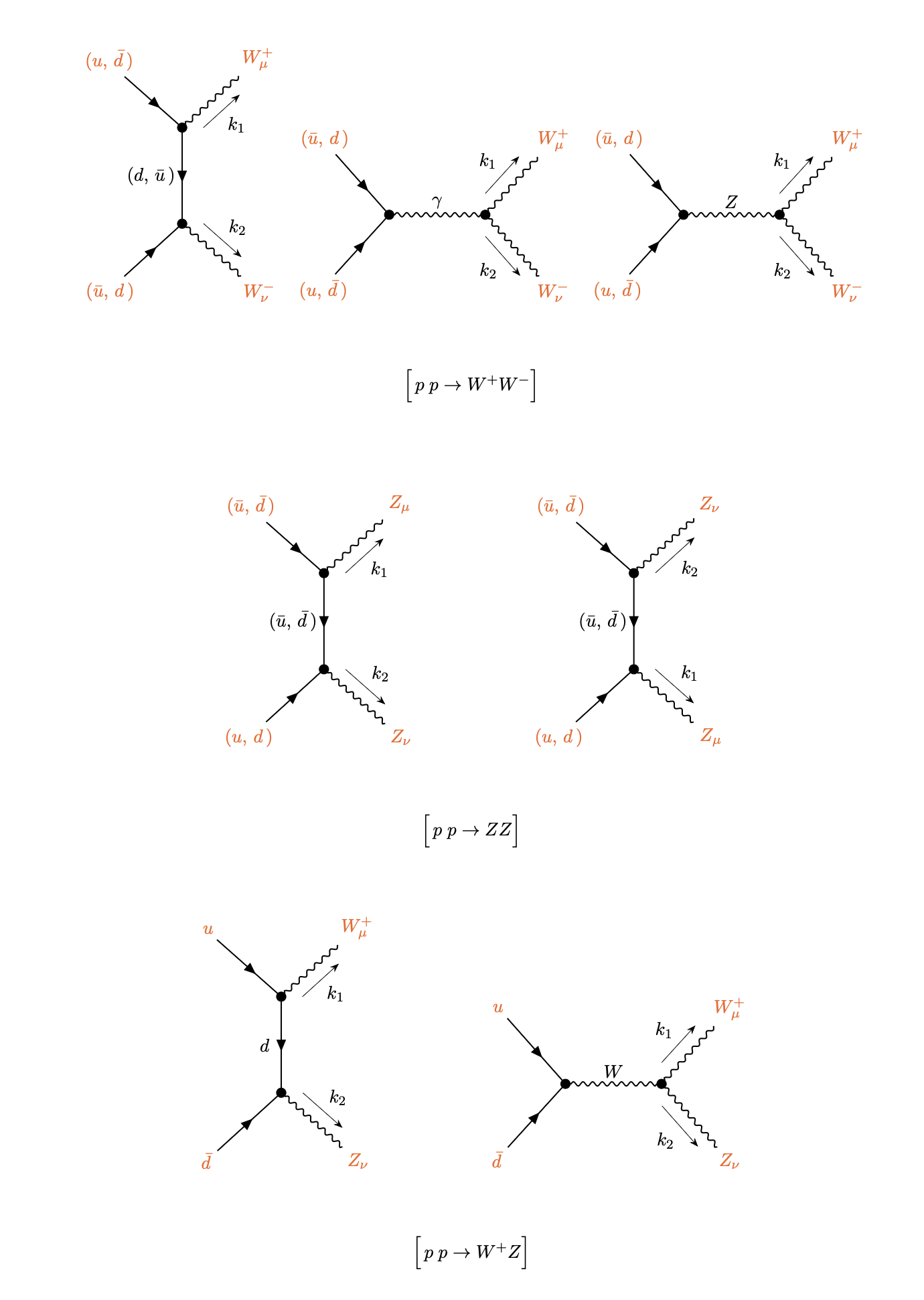
Figure 5.1: Feynman diagrams for the processes $p\;p\to W^{+}W^{-}$ (first row), $p\;p\to ZZ$ (second row) and $p\;p\to W^{+}Z$ (third row) at the parton level for the first quark generation. We neglect Diagrams mediated by the Higgs boson are neglected (in the limit of massless quarks). The arrows on the fermion lines indicate the momentum flow.

The polarization vectors of $W^{+}$ and $W^{-}$ are $\varepsilon^{\mu}(k_{1},\lambda_{1})$ and $\varepsilon^{\nu}(k_{2},\lambda_{2})$, respectively. The polarized amplitude for the process in Eq. (5.2), for $u$ and $\bar{u}$ initial states, is given by [131]

$${\cal M}^{u\bar{u}}_{WW}(\lambda_{1},\lambda_{2}) = -ie^{2}\Big{[}\bar{v}(p_{1})\Gamma^{\scriptscriptstyle{W}\scriptscriptstyle{W}}_{\mu\nu}u(p_{2})\Big{]}\varepsilon^{\mu}(k_{1},\lambda_{1})^{\star}\varepsilon^{\nu}(k_{2},\lambda_{2})^{\star}\,,$$ (5.3)

where the effective vertex $\Gamma^{WW}_{\alpha\beta}$ is

$$\Gamma^{\scriptscriptstyle{W}\scriptscriptstyle{W}}_{\mu\nu} = \frac{1}{s}\left(\gamma^{\alpha}\bar{g}_{V}^{q}-\gamma^{\alpha}\gamma_{5}\bar{g}_{A}^{q}\right)V_{\alpha\nu\mu}(q,-k_{2},-k_{1})+\frac{1}{4ts_{\scriptscriptstyle{W}}^{2}}\gamma_{\nu}\left(\not{p}_{2}-\not{k}_{1}\right)\gamma_{\mu}(1-\gamma_{5})\,,$$ (5.4)

with $\not{p}\equiv\gamma^{\mu}p_{\mu}$ and $s_{\scriptscriptstyle{W}}=\sin\theta_{W}$ and $e$ being the unit of electric charge. The effective couplings $\bar{g}^{q}_{V,A}$ are defined as

$$\bar{g}_{V}^{q}=Q^{q}+\frac{g_{V}^{q}\chi}{s_{\scriptscriptstyle{W}}^{2}}\,,~{}~{}\bar{g}_{A}^{q}=\frac{g_{A}^{q}\chi}{s_{\scriptscriptstyle{W}}^{2}}\,,~{}~{}\chi=\frac{s}{2(s-M_{Z}^{2})}\,,$$ (5.5)

where $g_{V}^{q}=T_{3}^{q}-2Q^{q}s_{\scriptscriptstyle{W}}^{2}$, $g_{A}^{q}=T_{3}^{q}$ and $T_{3}^{q}$ and $Q^{q}$ are the isospin and electric charge (in unit of $e$) of the quark $q$. The $\chi$ term in Eq. (5.5), which weights the contribution of the virtual $Z$ channel, is real since we neglect the $Z$ width contribution. The function $V_{\alpha\nu\mu}(k_{1},k_{2},k_{3})$ is the usual Feynman rule for the trilinear vertex $V_{\alpha}(k_{1})~{}W^{+}_{\nu}(k_{2})~{}W^{-}_{\mu}(k_{3})$, $V\in\{\gamma,Z\}$ with all incoming momenta (see [131] for its definition) and the Mandelstam variables are defined as

$$s=(p_{1}+p_{2})^{2},\quad t=(p_{1}-k_{1})^{2},\quad u=(p_{1}-k_{2})^{2}\,\,.$$ (5.6)

From the amplitude in Eq. (5.3), summing over the spin of quarks one obtains the compact expression

$${\cal M}^{u\bar{u}}_{WW}(\lambda_{1},\lambda_{2})\Big{[}{\cal M}^{u\bar{u}}_{WW}(\lambda_{1}^{\prime},\lambda_{2}^{\prime})\Big{]}^{{\dagger}}\,=\,\mbox{Tr}\,\Big{[}\bar{\Gamma}^{\scriptscriptstyle{W}\scriptscriptstyle{W}}_{\mu\nu}\,\not{p}_{1}\,\Gamma^{\scriptscriptstyle{W}\scriptscriptstyle{W}}_{\mu^{\prime}\nu^{\prime}}\,\not{p}_{2}\Big{]}\mathscr{P}^{\mu\mu^{\prime}}_{\lambda_{1}\lambda_{1}^{\prime}}(k_{1})\mathscr{P}^{\nu\nu^{\prime}}_{\lambda_{2}\lambda_{2}^{\prime}}(k_{2})\,,$$ (5.7)

where the symbol $\bar{\Gamma}_{\mu\nu}=\gamma_{0}(\Gamma_{\mu\nu})^{{\dagger}}\gamma_{0}$ and the projector $\mathscr{P}^{\mu\nu}_{\lambda\lambda^{\prime}}(k)$ is given in Eq. (3.27) with $M=M_{W}$.

The result for the $d\bar{d}\to W^{+}W^{-}$ process follows from Eq. (5.7) through the substitutions

$$\bar{g}_{V}^{u}\to-\bar{g}_{V}^{d},\quad\bar{g}_{A}^{u}\to-\bar{g}_{A}^{d},\quad\beta_{\scriptscriptstyle{W}}\to-\beta_{\scriptscriptstyle{W}}\,,$$ (5.8)

with the angle $\Theta$ being defined as before by the anti-quark and $W^{+}$ momenta. The contribution of strange quark initial states equals that of $d$ quarks in the considered massless limit.

Following the procedure explained in Section 3.2, from Eq. (5.7) (together with the corresponding ones for $d\bar{d}$ and $s\bar{s}$ processes) one can compute the unnormalized correlation coefficients $\tilde{f}_{a}$, $\tilde{g}_{a}$, and $\tilde{h}_{ab}$ of the density matrix for the process at and consequently, the expectation value of the operator ${\cal I}_{3}$ and the observable $\mathscr{C}_{2}$. The explicit expressions for $A^{q\bar{q}}$, $\tilde{h}_{ab}$ $\tilde{f}_{a}$, and $\tilde{g}_{a}$ as function of $m_{\scriptscriptstyle{W\!W}}$ and $\Theta$ can be found in the original work [131].

As explained in Section 2.3, for the observable ${\cal I}_{3}$ one can find at each point in the kinematic space the unitary matrices $U$ and $V$ that maximize the violation of Bell inequalities.

The results obtained in [131] for the two observables of interest, are reported in Fig. 5.2, as functions of the two kinematic variables $\Theta$ and $m_{\scriptscriptstyle{W\!W}}$. Comparable results are obtained in [133, 164]. From these results we can see that the violation of the Bell inequalities takes place only in a limited range of the kinematic variables, at higher $WW$ invariant mass and for scattering towards the transverse direction. The area in which ${\cal I}_{3}>2$ is indicated by the lighter-shaded area in plot on the left of Fig. 5.2. The explicit expression for the unitary $U$ and $V$ matrices (with accuracy at the percent level) that maximize the Bell observable in this particular kinematic region can be found in [131].

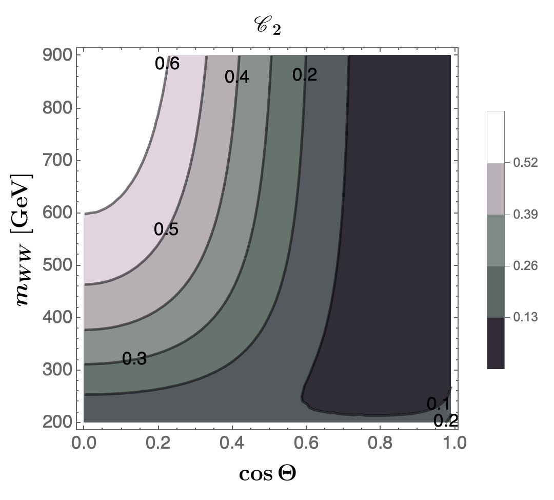
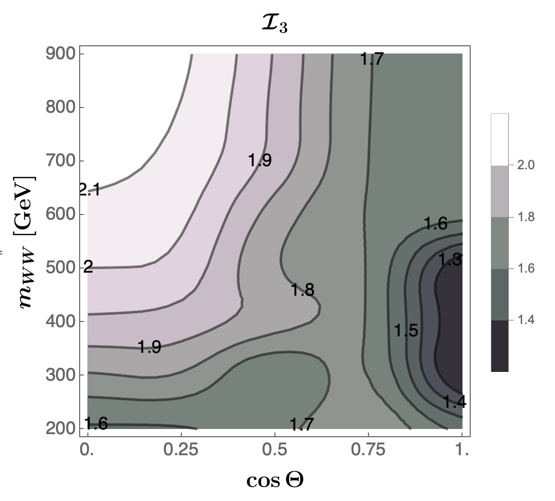
Figure 5.2: The observables $\mathscr{C}_{2}$ (left plot) and ${\cal I}_{3}$ (right plot) for the process $p\;p\to W^{+}W^{-}$ as functions of the invariant mass and scattering angle. Figures revisited from [131] (CC BY 4.0).

The observable $\mathscr{C}_{2}$ follows roughly the pattern of ${\cal I}_{3}$ and reaches the largest values in the upper-left quadrant, thus witnessing the presence of states more entangled than in the rest of the kinematic space. This feature can be made manifest by considering the density matrix of the process. For instance, by restricting to the region of maximum entanglement and Bell inequality violation, close to $m_{WW}=900$ GeV and $\cos\Theta=0$, the polarization density matrix for the $W^{+}W^{-}$ states can be approximated up to terms $O(10^{-3})$ by the following combination of pure state density matrices

$$\rho=\alpha\,|\Psi_{+-}\rangle\langle\Psi_{+-}|+\beta\,|\Psi_{+-\,0}\rangle\langle\Psi_{+-\,0}|+\gamma\,|00\rangle\langle 00|+\delta\,|\Psi_{0\,-}\rangle\langle\Psi_{0\,-}|\ ,$$ (5.9)

with decreasing weights: $\alpha\simeq 0.72$, $\beta\simeq 0.18$, $\gamma\simeq 0.07$ and $\delta\simeq 0.02$; the normalization condition $\alpha+\beta+\gamma+\delta=1$ is satisfied within the adopted approximation. The involved pure states are

$$|\Psi_{+-}\rangle=\frac{1}{\sqrt{2}}\big{(}|++\rangle-|--\rangle\big{)}\ ,$$

$$|\Psi_{0\,-}\rangle=\frac{1}{\sqrt{2}}\big{(}|0\,-\rangle+|-0\rangle\big{)}\ ,$$ (5.10)

$$|\Psi_{+-\,0}\rangle=\frac{1}{\sqrt{3}}\big{(}|++\rangle-|--\rangle+|0\,0\rangle\big{)}\ ,$$

where $|a\,b\rangle=|a\rangle\otimes|b\rangle$ with $a,b\in\{+,\,0,\,-\}$ are the polarization states of the two $W$ gauge bosons at rest in the single spin-1 basis. As we can see, the dominant contribution in (5.9) comes from the entangled pure state $|\Psi_{+-}\rangle$. This can justifies the high value of $\mathscr{C}_{2}$. However, by retaining all the terms including the ones of $O(10^{-3})$, the actual density matrix $\rho$ describes a mixture. This features explains why the corresponding value of $\mathscr{C}_{2}$, in this corner of the kinematic space, is large but far from maximal.

5.1.2   Computing the observables: $p\,p\to ZZ$

The tree-level Feynman diagrams contributing to the process

$$\bar{q}(p_{1})q(p_{2}) \to Z(k_{1},\lambda_{1})Z(k_{2},\lambda_{2})\,,$$ (5.11)

at the parton level are shown in the middle row of Fig. 5.1. We indicate the polarization vectors of the two $Z$ bosons with $\varepsilon^{\mu}(k_{1},\lambda_{1})$ and $\varepsilon^{\nu}(k_{2},\lambda_{2})$.

The polarized amplitude for the process in Eq. (5.11) is given by

$${\cal M}^{q\bar{q}}_{ZZ}(\lambda_{1},\lambda_{2}) = -\frac{ie^{2}}{4c_{\scriptscriptstyle{W}}^{2}s_{\scriptscriptstyle{W}}^{2}}\Big{[}\bar{v}(p_{1})\Gamma^{\scriptscriptstyle{Z}\scriptscriptstyle{Z}}_{\mu\nu}u(p_{2})\Big{]}\varepsilon^{\mu}(k_{1},\lambda_{1})^{\star}\varepsilon^{\nu}(k_{2},\lambda_{2})^{\star}\,,$$ (5.12)

where

$$\Gamma^{\scriptscriptstyle{Z}\scriptscriptstyle{Z}}_{\mu\nu}\,=\,V^{q}_{\mu}\frac{(\not{k}_{1}-\not{p}_{1})}{u}\,V^{q}_{\nu}+V^{q}_{\nu}\frac{(\not{k}_{1}-\not{p}_{2})}{t}V^{q}_{\mu}\,,$$ (5.13)

and

$$V^{q}_{\mu}\,=\,g_{V}^{q}\gamma_{\mu}-g_{A}^{q}\gamma_{\mu}\gamma_{5}$$ (5.14)

with the $g_{V,A}^{q}$ couplings defined as in Eq. (5.5).

Summing over the quark polarizations and colors we then obtain

$${\cal M}^{q\bar{q}}_{ZZ}(\lambda_{1},\lambda_{2})\Big{[}{\cal M}^{q\bar{q}}_{ZZ}(\lambda_{1}^{\prime},\lambda_{2}^{\prime})\Big{]}^{{\dagger}}\,=\,\mbox{Tr}\,\Big{[}\bar{\Gamma}^{\scriptscriptstyle{Z}\scriptscriptstyle{Z}}_{\mu\nu}\,\not{p}_{1}\,\Gamma^{\scriptscriptstyle{Z}\scriptscriptstyle{Z}}_{\mu^{\prime}\nu^{\prime}}\,\not{p}_{2}\Big{]}\mathscr{P}^{\mu\mu^{\prime}}_{\lambda_{1}\lambda_{1}^{\prime}}(k_{1})\mathscr{P}^{\nu\nu^{\prime}}_{\lambda_{2}\lambda_{2}^{\prime}}(k_{2})\,,$$ (5.15)

where $\mathscr{P}^{\mu\nu}_{\lambda\lambda^{\prime}}(k)$ is given in Eq. (3.27) with $M=M_{Z}$ and the symbol $\bar{\Gamma}_{\mu\nu}$ is defined as in Section 5.1.1.

The corresponding $f_{a},~{}g_{a}$ and $h_{ab}$ of the polarization density matrix, have been obtained in [131] and can be derived by following the same procedure as explained in Section 5.1.1. We report their expressions in appendix B for completeness.

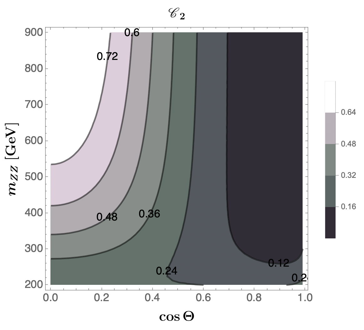
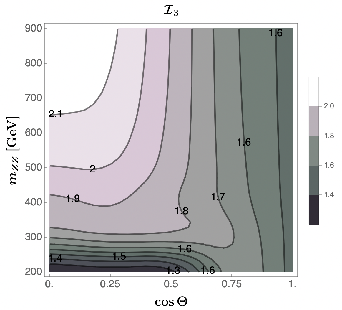
Figure 5.3: The observables $\mathscr{C}_{2}$ (left plot) and ${\cal I}_{3}$ (right plot) for the process $p\,p\to ZZ$ as functions of the invariant mass and scattering angle in the CM frame. Figures revisited from [131] (CC BY 4.0).

Fig. 5.3 shows the analytic results for the entanglement observables computed in [131]. As we could see from these results, the violation of the Bell inequalities for the $ZZ$ production takes place only in a limited range of the kinematic variables.

The observable $\mathscr{C}_{2}$ follows the pattern of ${\cal I}_{3}$—as it does in the case of the $W^{+}W^{-}$ final states—and again reaches the largest values in the upper-left quadrant. In this region it witnesses the presence of states more entangled than in the rest of the kinematic space.

5.1.3   Monte Carlo simulations of events

Monte Carlo simulations of diboson production at the LHC has been performed in [133] and [164]. The MadGraph5-_aMC@NLO [141] software is used including spin correlations and relativistic and Breit-Wigner effects. Events are generated at the leading order at CM energy of 13 TeV, and the 4-lepton final states considered.

Entanglement is proposed to be measured through the observable $\mathscr{C}_{2}$, Eq. (2.24), which provides a lower bound on the concurrence, and Bell inequality by means of the expectation value ${\cal I}_{3}$ of a version of the Bell operator (2.62), which is optimized along Cartesian planes. In agreement with the analytic results, entanglement is expected to be detected in the kinematic region of large scattering angles for invariant masses above 400 GeV for the $WW$ and $ZZ$ final states. For the tested observables Bell inequality violation is not predicted to reach a significant level even for a luminosity of 3 ab^-1 (Hi-Lumi) once the statistical uncertainty is taken into account.

5.2   Higgs boson decays into $WW^{*}$ and $ZZ^{*}$

The qutrits system of two massive gauge bosons is generated by the decay of the SM Higgs boson

$$h\to V(k_{1},\lambda_{1})\,V^{*}(k_{2},\lambda_{2})\,,$$ (5.16)

with $V\in\{W,Z$}, and $V^{*}$ regarded as an off-shell vector boson. We can treat the latter as an on-shell particle characterized by a fictitious mass

$$M_{V^{*}}=fM_{V}\,,$$ (5.17)

which is the original mass $M_{V}$ reduced by a factor $f$, with $0<f<1$. The Higgs boson is produced at the LHC as a resonance in the $s$-channel.

The expected quantum entanglement and Bell inequality violation for the processes $h\to WW^{*}$ has been analyzed in [69, 133], that for $h\to ZZ^{*}$ in [138, 133]. Comparable results have been obtained in [131] by using analytical results for the polarization density matrix of the two gauge bosons in the helicity basis. We summarize here first the analytical results of [138, 131] for the polarizations coefficients and its implications for quantum entanglement and Bell inequality violation observables. The corresponding results obtained by Monte Carlo simulation of events are briefly discussed in the next Section 5.2.2.

5.2.1   Computing the observables

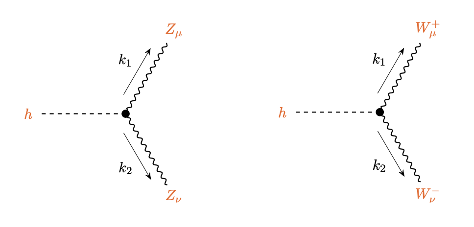
Figure 5.4: Feynman diagrams for the decay of the Higgs boson into a pair of massive gauge bosons.

The polarized amplitude for the Higgs boson decay in Eq. (5.16)) is given by

$${\cal M}(\lambda_{1},\lambda_{2})=g\,M_{V}\,\xi_{V}\,g_{\mu\nu}\varepsilon^{\mu\star}(k_{1},\lambda_{1})\varepsilon^{\nu\star}(k_{2},\lambda_{2})\,,$$ (5.18)

where $g$ is the weak coupling, $\xi_{W}=1$, and $\xi_{Z}=1/\cos{\theta_{W}}$ with $\theta_{W}$ the Weinberg angle. From the amplitude in Eq. (5.18) we obtain

$${\cal M}(\lambda_{1},\lambda_{2}){\cal M}(\lambda_{1}^{\prime},\lambda_{2}^{\prime})^{{\dagger}} = g^{2}\,M_{V}^{2}\,\xi^{2}_{V}\,g_{\mu\nu}g_{\mu^{\prime}\nu^{\prime}}\mathscr{P}^{\mu\mu^{\prime}}_{\lambda_{1}\lambda_{1}^{\prime}}(k_{1})\mathscr{P}^{\nu\nu^{\prime}}_{\lambda_{2}\lambda_{2}^{\prime}}(k_{2})\,.$$ (5.19)

where $\mathscr{P}^{\mu\nu}_{\lambda\lambda^{\prime}}(k)$ is given in Eq. (3.27) with $M=M_{V}$ or $M=M^{*}_{V}$ for the on-shell and off-shell boson, respectively.

Following the procedure explained in section 3 for a CM energy $\sqrt{s}=m_{h}$, one can obtain the coefficients $f_{a}$, $g_{a}$, and $h_{ab}$ ($a,b\in\{1,\dots,8\}$). These coefficients have been computed in [131] and their expression can be found in Appendix B.4. No dependence is expected of these coefficients on the scattering angle $\Theta$ because we are considering the decay of the scalar Higgs boson at rest.

The main theoretical uncertainty affecting the correlation coefficients in Eq. (B.15) is due to the missing next-to-leading electroweak corrections to the tree-level values. In [131] it was estimated that the error induced by these missing corrections yields at most a few percent of uncertainty on the main entanglement observables, in the relevant kinematic regions in which one of the two electroweak gauge boson are on-shell. This expectation is based on the fact that these corrections give a 1-2% effect on the total width  [169].

The polarization density matrix $\rho$ for the two vector bosons emitted in the decay of the Higgs boson is calculated to be [131]

$$\rho=2\begin{pmatrix}0&0&0&0&0&0&0&0&0\\ 0&0&0&0&0&0&0&0&0\\ 0&0&h_{44}&0&h_{16}&0&h_{44}&0&0\\ 0&0&0&0&0&0&0&0&0\\ 0&0&h_{16}&0&2\,h_{33}&0&h_{16}&0&0\\ 0&0&0&0&0&0&0&0&0\\ 0&0&h_{44}&0&h_{16}&0&h_{44}&0&0\\ 0&0&0&0&0&0&0&0&0\\ 0&0&0&0&0&0&0&0&0\\ \end{pmatrix}\,,$$ (5.20)

with the condition $\mbox{Tr}\,[\rho_{H}]=1$ following from the relation $4(h_{33}+h_{44})=1$. There are therefore only two independent coefficients under these assumptions.

In [138] the spin density matrix of the system is written in terms of tensor components $T^{L}_{M}$ (see Section 3) and the correlation coefficients entering the density matrix are indicated as $C_{L_{1},M_{1},L_{2},M_{2}}$ (see Eq. (3.47)). These coefficients are related to those in Eq. (5.20) by the correspondence

$$\frac{1}{6}C_{2,2,2,-2}=h_{44}\quad\text{and}\quad\frac{1}{6}C_{2,1,2,-1}=h_{16}\,.$$ (5.21)

Assuming that the state is pure, there would be entanglement if and only if the two components in Eq. (5.21) are different from zero.

Although some $f_{a}$ and $g_{a}$ are non-vanishing, the dependence of $\rho_{H}$ on these quantities cancels in the final expression. Furthermore, due to the following identity among the correlation coefficients $h_{44}=2\left(h_{16}^{2}+2h_{44}^{2}\right)$ the above polarization density matrix is idempotent

$$\rho^{2}=\rho\,,$$ (5.22)

as expected from the assumption that the final $VV^{*}$ state is a pure state. The density matrix in Eq. (5.20) can then be written as  [138]

$$\rho=|\Psi\rangle\langle\Psi|\,,$$ (5.23)

where (in the basis $|\lambda\,\lambda^{\prime}\rangle=|\lambda\rangle\otimes|\lambda^{\prime}\rangle$ with $\lambda,\lambda^{\prime}\in\{+,0,-\}$)

$$|\Psi\rangle=\frac{1}{\sqrt{2+\varkappa^{2}}}\left[|{\small+-}\rangle-\varkappa\,|{\small 0\,0}\rangle+|{\small-+}\rangle\right]$$ (5.24)

with

$$\varkappa=1+\frac{m_{h}^{2}-(1+f)^{2}M_{V}^{2}}{2fM^{2}_{V}}$$ (5.25)

and $\varkappa=1$ corresponding to the production of two gauge bosons at rest.

If one makes the assumption that the diboson system is described by a pure state, then one can measure its entanglement through the entropy of entanglement defined in Eq. (2.16). This quantity is plotted in Figs. 5.5 and 5.6 as a function of the mass of virtual $W$ or $Z$ boson [131]. As we can see from these calculations, the entropy of entanglement is expected to reach its maximum at the kinematic threshold, signaling a maximally entangled state. The dependence of the polarization entanglement on the mass of the virtual state is due the contribution of the longitudinal polarization, parametrized by the coefficient $\varkappa$ in Eq. (5.24). Indeed, this contribution starts out bigger and decreases to 1 at the threshold. The value of 1 corresponds to a pure singlet state and thus to the maximum in the entanglement of the state.

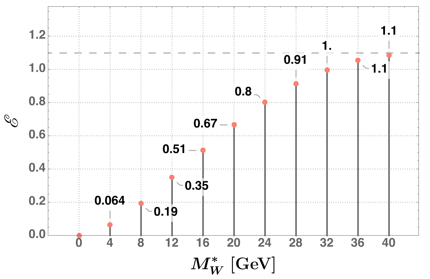
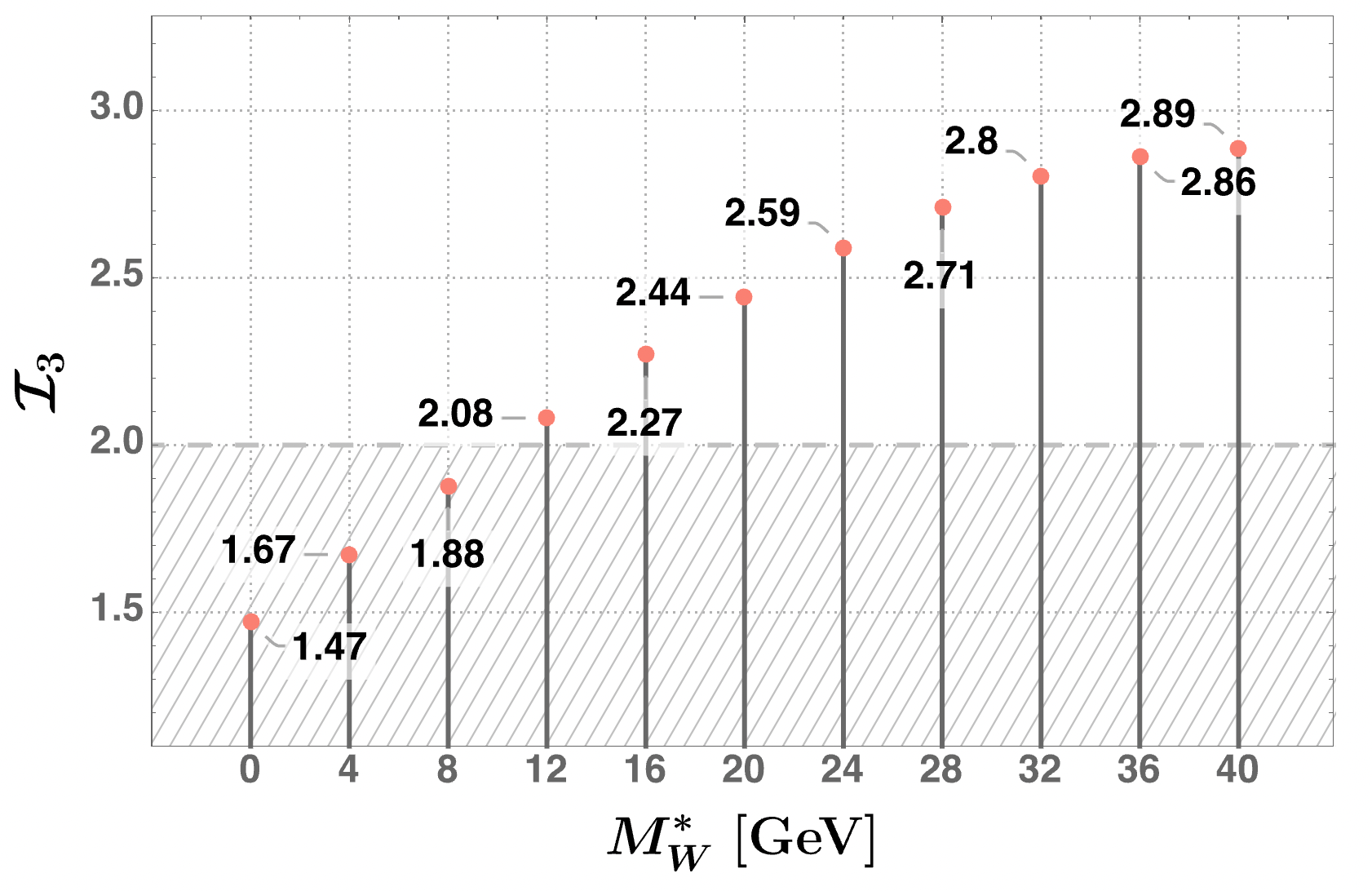
Figure 5.5: Predictions of the entropy of entanglement ${\cal E}$ (left plot) and the Bell operator expectation value ${\cal I}_{3}$ (right plot) for the pair production of $W$ bosons in Higgs boson decays as functions of the virtual $W^{*}$ mass in the range $0<M_{W^{*}}<40$ GeV [131]. The dashed horizontal line in the right-hand side plot marks the Bell-inequality violation condition ${\cal I}_{3}>2$. The dashed line in the left-hand side plot denotes the maximum value of $\ln 3$. Figures revisited from [131] (CC BY 4.0).

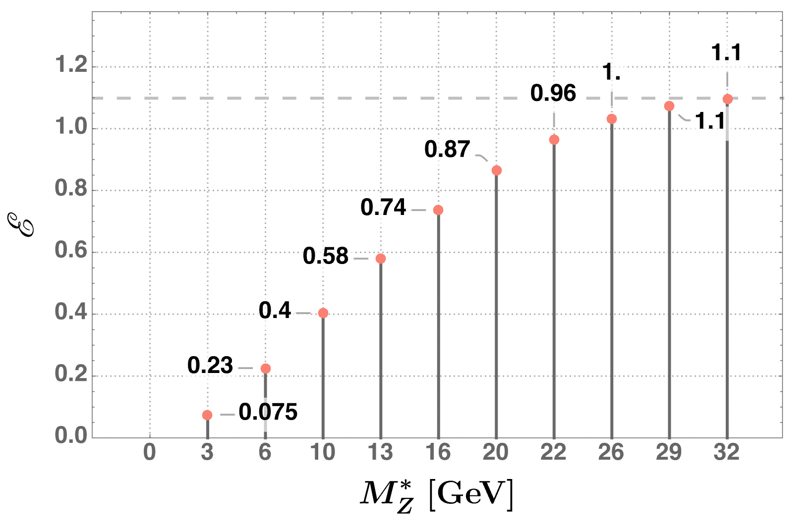
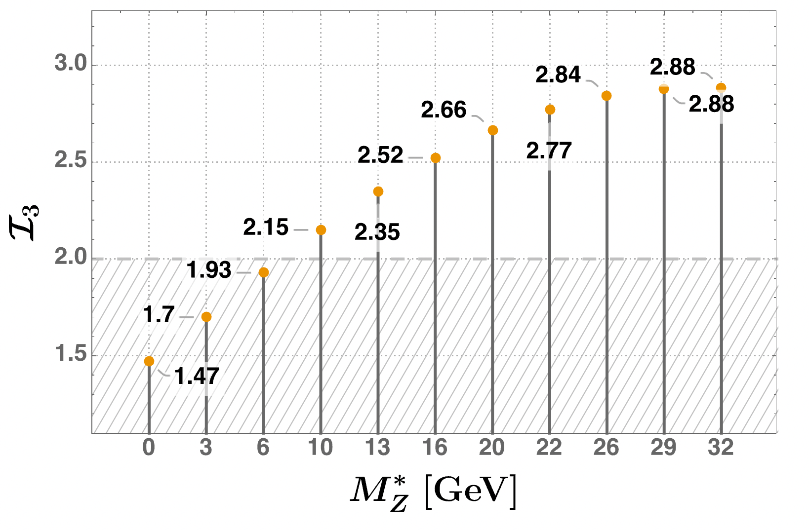
Figure 5.6: Predictions of the entropy of entanglement ${\cal E}$ (left plot) and the Bell operator expectation value ${\cal I}_{3}$ (right plot) for the pair production of $Z$ bosons in Higgs boson decays as functions of the virtual $Z^{*}$ mass in the range $0<M_{Z^{*}}<32$ GeV [131]. The dashed line in the left-hand side plot denotes the maximum value of $\ln 3$. Figures revisited from [131] (CC BY 4.0).

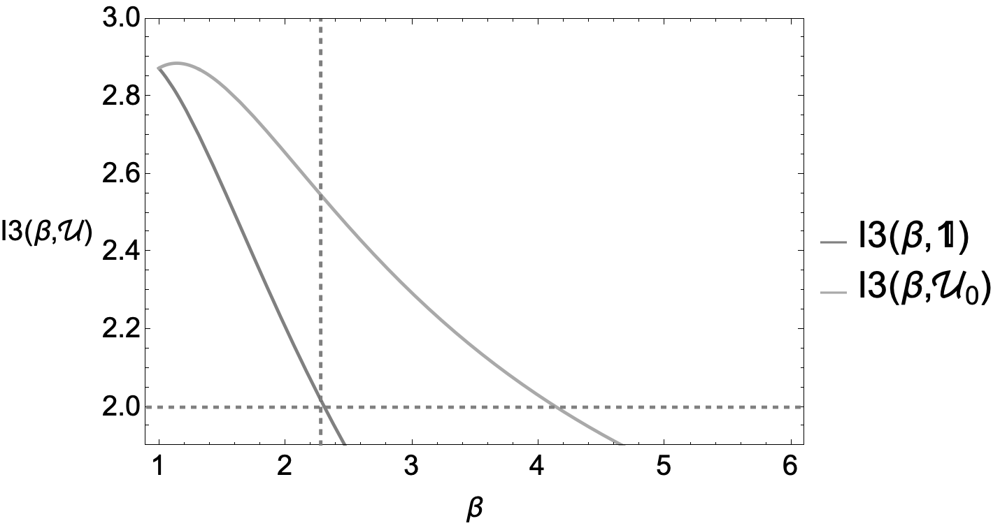
Figure 5.7: Expectation values of unoptimised (lower curve) and unitary-operator optimised (upper curve) Bell operators for $H\rightarrow ZZ$ decays as a function of the relative coefficient $\beta$ ($\varkappa$ in Eq. (5.24)) of the longitudinal polarisation of the state. Figure from [138] (CC BY 4.0).

The maximization of the ${\cal I}_{3}$ observable, which depends in this case only on the $M_{V}^{*}$ mass, is obtained through the unitary rotation in Eq. (2.64) of the $\mathscr{B}$ matrix in Eq. (2.62), that maximizes the value of the corresponding expectation value. This maximization must be performed point by point as the density matrix varies with $M_{V}^{*}$. The unitary matrices that maximizes the ${\cal I}_{3}$ observable in the last bins (in which $M_{W^{*}}=40$ GeV and $M_{Z^{*}}=32$ GeV) for the $h\to WW^{*}$ and $h\to ZZ^{*}$ decays are given in [131].

The plots on the left-hand side in Figs. 5.5 and 5.6 nicely show that the value of the entropy of entanglement Eq. (2.16) is expected to decrease as the pure state in Eq. (5.20) becomes less and less entangled, for decreasing values of $M^{*}_{V}$. The advantages obtained from using the optimal Bell operator can be seen in Figure 5.7. The relative coefficient $\beta$ of the longitudinal component to the polarisation increases is unity when the when the $Z$ bosons are produced at rest in their zero-momentum frame (ZMF), and increases at larger relative momenta.

The same Figs. 5.5 and 5.6 show the calculations for the Bell operator expectation value ${\cal I}_{3}$ (right panels) in the $h\to WW^{*}$ and $h\to ZZ^{*}$ decays. The plots are for different values of the virtual gauge boson masses $M_{{W}^{*}}$ and $M_{{Z}^{*}}$, respectively. The Bell inequality violation in $WW^{*}$ and $ZZ^{*}$ final states starts above 12 GeV and 10 GeV for $M_{W^{*}}$ and $M_{Z^{*}}$ invariant masses respectively, reaching its maximum allowed value of order ${\cal I}_{3}\sim 2.9$ at the largest invariant mass of the corresponding off-shell gauge boson.

5.2.2   Monte Carlo simulations of events

The simulation for the process $h\to WW^{*}$ has been performed in [69] in which most of the tools for the analysis of qutrit systems (as discussed in Section 3) were introduced as well. The MadGraph5_aMC@NLO [141] software is used including spin correlations and relativistic and Breit-Wigner effects. The Bell operator ${\cal I}_{3}$ is optimized along Cartesian planes. Only the fully leptonic decays are considered. There are two neutrinos in the final state and the reconstruction of the rest frame of each gauge boson necessarily introduces a potentially large uncertainty. Various scenarios about the overall uncertainty are discussed (by attributing a smearing in the value of the lepton momenta) and the significance for the Bell inequality violation shown to vary from about 5$\sigma$ (for the most optimistic momenta reconstruction) to 1$\sigma$ (for a less sanguine one) at the luminosity of 140 fb^-1 at the LHC.

The same decay is discussed in [170] by looking at the semi-leptonic decay $h\to jj\ell\nu_{\ell}$ (rather than the fully leptonic one). The momentum from the $s$-jet (identified via the $c$-tagging of the companion jet) is used to measure the polarization of one of the two $W$-bosons. It has been shown that the efficiency of the jet tagging and the decreased uncertainty in the single neutrino momentum may improve the polarization reconstruction.

The process $h\to ZZ^{*}$ has been simulated in [165, 133] and analyzed using tensor [165] and Gell-Mann [133] bases. There are no neutrinos in the final state and the rest frame of the gauge bosons can be reconstructed with precision. The basis that maximizes the Bell operator is explicitly written out in [165]. The MadGraph5_aMC@NLO [141] software is used to generate the events. It is found that, for a luminosity of 3 ab^-1 (Hi-lumi at the LHC), the significance for the violation of the Bell inequality can be as large as 4.5$\sigma$. This process is actually the most promising to test the Bell inequality in weak boson decays because of the clean reconstruction and low background.

5.3   Vector-boson fusion

Processes in which vector-boson fusion takes place, as in

$$W^{+}W^{-}\to W^{+}W^{-}\,,\quad Z\gamma\to W^{+}W^{-}\quad\text{or}\quad\gamma\gamma\to W^{+}W^{-}$$ (5.26)

have been analyzed in [171] by means of the computation of the corresponding tree level amplitudes within the SM. It is interesting that this family of scattering process contains final states with two quibits (photons), one qubit and one qutrit (photon and massive gauge bosons) and two qutrits (massive gauge bosons).

As before for other process, the amount of entanglement depends on phase space. More or less all channels share a comparable amount of entanglement but for the $ZZ\to ZZ$, whose entanglement is suppressed.

The violation of Bell inequality can be tested in vector-boson fusion by measuring the expectation value of the appropriated Bell operator in regions of the phase space that are identified and listed in [171].

5.4   $B$-meson decays in two vector mesons

The decays of the neutral $B$-mesons into two spin-1 mesons closely resemble those of the Higgs boson and the same tools can be put to work.

There are three helicity amplitudes for the decay of a scalar, or pseudo-scalar, into two massive spin-1 particles:

$$h_{\lambda}=\langle V_{1}(\lambda)V_{2}(-\lambda)|{\cal H}|B\rangle\quad\text{with}\quad\lambda=(+,\,0,\,-)\,,$$ (5.27)

and ${\cal H}$ is the interaction Hamiltonian giving rise to the decay. For the spin quantization axis ($\hat{z}$) we can use the direction of the momenta of the decay products in the $B^{0}$ rest frame. Helicities are here defined with respect to the $\hat{z}$ direction in the rest frame of one of the two spin-1 particles and $(+,\,0,\,-)$ is a shorthand for $(+1,\,0,\,-1)$.

The polarizations in the decay are described by a quantum state that is pure for any values of the helicity amplitudes [131, 172]. This state can be written as

$$|\Psi\rangle=\frac{1}{\absolutevalue{\mathcal{M}}}\Big{[}h_{+}\,|V_{1}(+)V_{2}(-)\rangle+h_{0}\,|V_{1}(0)V_{2}(0)\rangle+h_{-}\,|V_{1}(-)V_{2}(+)\rangle\Big{]}\,,$$ (5.28)

with

$$\absolutevalue{\mathcal{M}}^{2}=|h_{0}|^{2}+|h_{+}|^{2}+|h_{-}|^{2}\,.$$ (5.29)

The relative weight of the transverse components $|V_{1}(+)V_{2}(-)\rangle$ and $|V_{1}(-)V_{2}(+)\rangle$ with respect to the longitudinal one $|V_{1}(0)V_{2}(0)\rangle$ is controlled by the conservation of angular momentum. In general, only the helicity is conserved and the state in Eq. (5.28) belongs to the $J_{z}=0$ component of the $S=0,1$ or $2$ states.

The polarization density matrix $\rho=|\Psi\rangle\langle\Psi|$ can be written in terms of the helicity amplitudes as

$$\small\rho=\frac{1}{\absolutevalue{\mathcal{M}^{2}}}\,\begin{pmatrix}0&0&0&0&0&0&0&0&0\\ 0&0&0&0&0&0&0&0&0\\ 0&0&h_{+}h_{+}^{*}&0&h_{+}h_{0}^{*}&0&h_{+}h_{-}^{*}&0&0\\ 0&0&0&0&0&0&0&0&0\\ 0&0&h_{0}h_{+}^{*}&0&h_{0}h_{0}^{*}&0&h_{0}h_{-}^{*}&0&0\\ 0&0&0&0&0&0&0&0&0\\ 0&0&h_{-}h_{+}^{*}&0&h_{-}h_{0}^{*}&0&h_{-}h_{-}^{*}&0&0\\ 0&0&0&0&0&0&0&0&0\\ 0&0&0&0&0&0&0&0&0\\ \end{pmatrix}\,,$$ (5.30)

on the basis given by the tensor product of the polarizations $(+,\,0,\,-)$ of the produced spin-1 particles.

The polarizations of the spin-1 massive particles can be reconstructed using the momenta of the final charged mesons and leptons in which they decay [34]. Usually, the experimental analysis provides the polarization amplitudes. These are mapped into the helicity amplitudes by the correspondence

$$\frac{h_{0}}{\absolutevalue{\mathcal{M}}}=A_{0}\,,\quad\frac{h_{+}}{\absolutevalue{\mathcal{M}}}=\frac{A_{\parallel}+A_{\perp}}{\sqrt{2}}\,,\quad\frac{h_{-}}{\absolutevalue{\mathcal{M}}}=\frac{A_{\parallel}-A_{\perp}}{\sqrt{2}}\,.$$ (5.31)

The entanglement entropy and the Bell operator ${\cal I}_{3}$ can be readily be computed, the latter one after the optimization procedure of Eq. (2.64).

Data from the $B$-factories have been analyzed by the LHCb and Belle collaborations in terms of polarization amplitudes and provide an abundant source of processes in which it is possible to search for entanglement and test Bell inequality violation. Let us stress that the data and the analyses are already published and only the recasting in terms of entanglement markers and test of the Bell inequality need to be validated by the experimental Collaborations.

The decay for which the most precise polarization amplitudes are known is $B^{0}\to J/\psi\,K^{*}(892)^{0}$ [173] for which, under the assumption that the density matrix takes the form Eq. (5.30), it can be found [168] that

$$\mathscr{E}=0.756\pm 0.009\,\quad\text{and}\quad{\cal I}_{3}=2.548\pm 0.015\,,$$ (5.32)

with a significance well in excess of 5$\sigma$ (numerically $36\sigma$) for the violation of the Bell inequality ${\cal I}_{3}<2$.

To close the locality loophole—which exploits (see Section 6) events not separated by a space-like interval, as it is the case of the $J/\psi\,K^{*}$ decays—one must consider decays in which the produced particles are identical, as in the $B_{s}\to\phi\phi$ decay, and therefore their life-times are also the same. The actual decays take place with an exponential spread, with, in the $\phi\phi$ case, more than 90% of the events being separated by a space-like interval.

For the decay $B_{s}\to\phi\phi$ [174], it is found [168] that

$$\mathscr{E}=0.734\pm 0.037\,\quad\text{and}\quad{\cal I}_{3}=2.525\pm 0.064\,,$$ (5.33)

with a significance of $8.2\sigma$ for the violation of the Bell inequality ${\cal I}_{3}<2$.

There is another reason why the decays of the $B$-mesons are interesting in testing for the presence of entanglement. It is possible to extract from the data [173, 174] the strong phases arising from the final-state interactions in the $B$-meson decays and compute their contribution to the polarization amplitudes. We therefore know for the same process the amount of entanglement arising from the weak interactions, which are responsible for the decay, as well as that from the strong interactions in the subsequent re-scattering. The contribution to the latter can be measured and shown to increase the overall entanglement between the spins of the decay products.

6   Possible loopholes in testing Bell inequality at colliders

As pointed out in the Section 1.3 of the Introduction, soon after the first test of Bell inequality was performed, ways to escape the consequences were put forward. Since then, these attempts have been grouped together under the label of ‘loopholes’.

The existence of a loophole in the test of Bell inequality shows how to avoid the exclusion of deterministic, local theories even in the presence of an experimentally verified violation of the inequality. A violation of the inequality that is free of loopholes excludes these theories and confirms quantum mechanics. If the test is open to one or more loopholes, the possibility of a description in terms of local, deterministic models is, in principle, still possible.

The discussion of loopholes has taken place so far mostly in the framework of experiments in optics and atomic physics. It is important to bear in mind that (almost) all possible loopholes have been closed in low-energy tests with photons [43, 42] and in atomic physics [45]. This means that devising a local hidden variable model – be it deterministic or stochastic – exploiting any or all of these loophole is nowadays a formidable if not indeed impossible task.

The extension to collider physics of any discussion about possible loopholes is delicate and still little explored [144, 151]. The implications for collider experiments of Bell-violation measurements and considerations of the possible dependencies on hidden variables was recently considered in the philosophy of physics literature [175].

We note that the existence of a loophole does not mean that a test of the Bell inequality is useless or meaningless. The test and the loophole are two distinct entities and the existence of a loophole only implies that there exists, in principle, a way to bypass the ruling out of locally local hidden variable models. At the same time, the hypothetical model, required to exploit the loophole, is necessarily made rather complicated and unnatural by its accounting for the violation. Indeed, all these models have to satisfies so involved a series of requirements that they are very difficult to conceive and very few of them have even be actually defined.

Contrary to experiments at low energies, those at colliders were not designed to test Bell violation and therefore seem more prone to loopholes and other shortcomings. Nevertheless, as we discuss below, most loopholes appear to be closed already by the current most common settings of collider detectors.

The potential loopholes that could be present in any test of Bell inequality are:

• Detection loophole [178]: If the efficiency in detecting the entangled states is not 100%, the undetected states could, had they been taken into account, restore the inequality;

• Locality loophole [95]: Bell locality, even if satisfied, could be bypassed if it is possible for the entangled states to communicate by means of a local interaction;

• Coincidence loophole [179]: The states are misidentified and do not belong to the entangled pair;

• Freedom of choice loophole [180]: The lack of freedom in choosing the measurement to be performed alters the outcome;

• Super-determinism loophole [181]: if the initial conditions fully predict all successive developments, possible experiments included, Bell locality is always satisfied.

How do these loopholes affect a test of Bell inequality at colliders?

• The detection loophole is always present at colliders where only a small fraction of the final states are actually recorded. Here one must appeal to the assumption of having a fair sampling of these events. This is what is routinely assumed in high-energy physics since also a measurement of a cross section or branching ratio would be open to the same loophole. Given such an assumption, due to the high efficiency of the detectors at colliders, as far as the measure of the momenta of charged particles, the detection loophole might be closed. For qubits the loophole would be closed if the efficiency were more than about 80% [38] and this requirement is even lower for states belonging to larger Hilbert spaces [182]. By comparison, the efficiency of the LHCb detector is more than 90% [183] for kaon, pion and muon identification. However analysis selection efficiencies would also need to be considered.

• The locality loophole is potentially present for states made of particles that end up decaying with a relative time-like interval, either because they decayed at different times or because they do not move apart fast enough. It could be particularly serious in the case of charged particles for which the electromagnetic interaction can be used in bypassing the test. Fig. 6.1 shows the kinematics exploited by the locality loophole. To close the locality loophole it is desirable to consider decays in which the produced particles are identical, and therefore their life-times are also the same. Even in this case, the actual decays take place with an exponential spread. To take this into account, one must verify that the majority of the events do take place separated by a space-like interval and/or weed out those that do not.

  

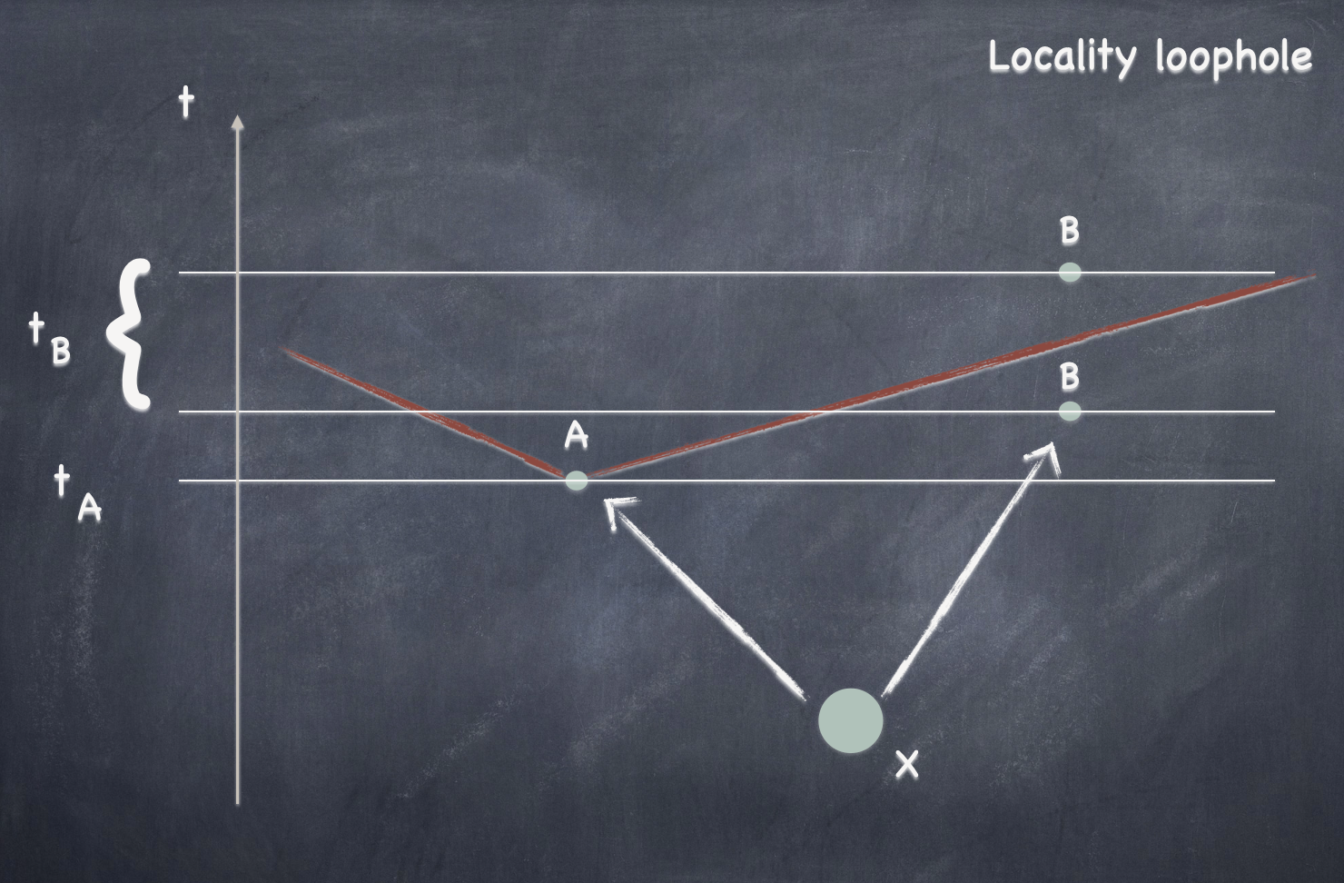
  Figure 6.1: Kinematics of the locality loophole. Particle B can decay within the future cone of particle A either because of a longer lifetime or because the random spread in its decay time.

  Fig. 6.2 shows a typical distribution of decays events as a function of their relative distances. The relative velocity $v$ with which the pair flies apart is sufficiently large to create, at the times $t_{1}$ and $t_{2}$ of decay, a space-like separation iff

  $$\frac{|t_{1}-t_{2}|\,c}{(t_{1}+t_{2})\,v}<1\,.$$ (6.1)

  The separation prevents local interactions (as those arising through the exchange of photons between charged particles) and ensures that the locality loophole is closed [184]. The selection of these events could be implemented with a suitable cut on the relative momentum of the two particles. If the amount of available data is large and the fraction of pairs rejected by the cut is small, this refinement would not affect the significance of the Bell test under consideration.

  

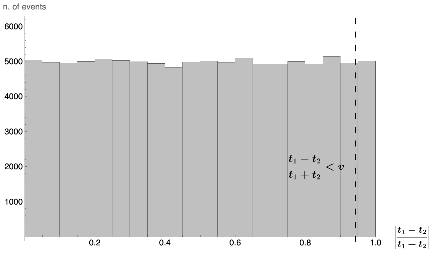
  Figure 6.2: Example about the fraction of events separated by a space-like interval (95% in this histogram). Histogram of the number of events as a function of the ratio $|t_{1}-t_{2}|/(t_{1}+t_{2})$ between the difference and the sum of the decay times of the two taus. The events have been generated by $10^{5}$ pseudo-experiments in which the decay times are randomly varied within an exponential distribution. The black-dashed vertical line distinguishes events separated by a time-like interval (to the right of the line) from those that are space-like separated (to the left of the line). Figure revisited from [151] (CC BY 4.0)

• The coincidence loophole does not seems to be problematic at colliders. Such a misidentification is always accounted for in the quoted uncertainty in the results of the experiments.

• The freedom-of-choice loophole relates to the possible dependence of is—depending on whom you ask—either the hardest or the simplest to close at a collider setting. At low-energy experiments the loophole is addressed by coupling the polarization measurement to a (pseudo)random choice that is made after the entangled states have been produced, and with a space-like separation at the point of ‘choice’. This is not possible at colliders where the detector is fixed by its construction design. Though this seems to be a show stopper, we have advanced an alternative point of view: the polarization measurement is made inside the detector by the particles themselves as they decay into the final state; because the decay is a quantum process, it is the ultimate random process and one could argue that therefore the freedom of choice is implemented. It can be argued that the objection that the quantum theory one would like to put to the test is employed in closing the loophole can be extended also to the (pseudo)random choice in the loophole-free low-energy setting. Be that as it may, as our brief discussion reveals, the physics surrounding this loophole is not settled yet and needs further discussion.

• The ‘super-determinism’ loophole is related; a dependence of the measurement outcomes on information in the overlapping past light-cones of the respective measurements can break the assumed form of the probability distribution Eq. (2.35). This loophole cannot be closed at colliders, nor can it be be closed in atomic-physics experiments or, indeed, at all.

The discussion of the role of loopholes in the violation of Bell inequality at high energies is still at its first steps [175]. It is fair to say that models exploiting these loopholes to save local hidden variable theories – either deterministic or stochastic – will become even harder to define once the violation will be extended at colliders and in the presence of strong and electroweak forces because they will have to account for both the low- and the high-energy experiments. We are not aware of any definite model claiming to be able to do that.

7   Probing new particles and fields with entanglement

The sensitivity of entanglement on the specific form of the couplings between the states produced at colliders makes it a promising observable to be used in constraining new physics – particles, fields and interactions – beyond the SM. The overall advantage in sensitivity with respect to a more usual observable like the cross section is tempered by the added uncertainty necessarily present in the determination of the polarizations. Yet the use of entanglement can contribute to better constrain interactions and models beyond the SM, as the examples reviewed below show. This is a field still in its infancy but we expect quantum state tomography to become part of the routine tools in the physical analysis of the experimental events.

7.1   Top quark

The SM Effective Field Theory (SMEFT) expansion parametrizes possible new particles and fields, characterized by heavy new states, in terms of operators that are obtained by integrating out these new states. Modifications of the entanglement of the spins of top-quark pairs in this framework has been studied in [185]. In this approach the effective Lagrangian is given by

$${\cal L}_{\text{\tiny SMEFT}}={\cal L}_{\text{\tiny SM}}+\frac{1}{\Lambda^{2}}\sum_{i}c_{i}{\cal O}_{i}\,,$$ (7.1)

in which, at the leading order in QCD, all $CP$-even operators of dimension six are included. There is 1 operator with zero fermions, 2 operators with two fermions and 14 with four fermions (see [185] for their explicit form). In Eq. (7.1), $\Lambda$ is the scale of the effective theory (roughly the mass of the heavy states) and $c_{i}$ the Wilson coefficients of the corresponding operators.

The concurrence is modified by the presence in the differential cross section of terms linear in $c_{i}/\Lambda$ (arising from the interference between the SM and the dimension six operators) and by terms quadratic in $c_{i}/\Lambda$ (arising from the square of the dimension six operators). The qualitative result of the analysis is that at threshold the linear interference terms modify very little the concurrence while the quadratic terms reduce it. Both classes of terms reduce the concurrence in the high-energy regime by a sizable amount.

The impact of higher-order terms in the SMFET expansion have been studied in [186].

7.1.1   Gluon magnetic-like dipole moment

To show how entanglement can provide constraints on higher-order operators, let us focus on a single one, the gluon magnetic-like dipole operator, as discussed in [140], which gives rise to the effective Lagrangian

$${\cal L}_{\text{\tiny dipole}}=\frac{c_{\,tG}}{\Lambda^{2}}\big{(}{\cal O}_{tG}+{\cal O}_{tG}^{\dagger}\big{)}\quad\text{with}\quad{\cal O}_{tG}=g_{s}\left(\bar{Q}_{L}\,\sigma^{\mu\nu}\,T^{a}\,t_{R}\right)\tilde{H}G_{\mu\nu}^{a}\,.$$ (7.2)

In Eq. (7.2) above, $Q_{L}$ and $t_{R}$ stands for the $SU(2)_{L}$ left-handed doublet of top-bottom quarks and right-handed top quark fields respectively, while $\tilde{H}$ is as usual the dual of the $SU(2)_{L}$ doublet Higgs field, with SM vacuum expectation value $v$ given by $\langle 0|\tilde{H}|0\rangle=(v/\sqrt{2},0)$.

The magnetic-like dipole moment is given by

$$\mu=-\frac{\sqrt{2}m_{t}v}{\Lambda^{2}}c_{\,tG}\ .$$ (7.3)

The addition of an effective magnetic dipole moment term to the SM Lagrangian, gives rise in general to further mixture contributions, thus weakening the entanglement of the $t\bar{t}$ spin state produced by the SM interaction. It is this loss of entanglement both in the $q\bar{q}$ and $gg$ production channels that allows the bound on the magnitude of the extra, effective parameter $\mu$, to be obtained.

By running a simple Monte Carlo, the authors of [140] find that—in the kinematic region $m_{t\bar{t}}>900$ GeV and $2\Theta/\pi>0.85$, where the relative difference between the SM and the new physics is largest and equal to about 3%—a separation of 2.3$\sigma$ is possible down to the value of $\mu=0.003$ with the data of run 2 at the LHC. This result is in agreement with what found in [185] (with $c_{tG}=-0.1$ for $\Lambda=1\,\text{TeV}$) and compares favorably with current determinations [187, 188] which find a bound around $\mu=0.02$.

7.2   $\tau$ lepton

Quantum state tomography has been used in the study of the properties of the $\tau$ lepton and its coupling to quarks and the Higgs boson.

7.2.1   Contact interactions

Contact interactions in $\tau$-pair entanglement were discussed in [140]. The most general contact operators for the production of $\tau$-leptons from quarks can be written, in chiral components, as

$${\cal L}_{\text{\tiny cc}}= -\frac{4\pi}{\Lambda^{2}}\eta_{LL}(\bar{q}_{L}\gamma^{\alpha}q_{L})\,(\bar{\tau}_{L}\gamma_{\alpha}\tau_{L})-\frac{4\pi}{\Lambda^{2}}\eta_{RR}(\bar{q}_{R}\gamma^{\alpha}q_{R})\,(\bar{\tau}_{R}\gamma_{\alpha}\tau_{R})$$ (7.4)

$$-\frac{4\pi}{\Lambda^{2}}\eta_{LR}(\bar{q}_{L}\gamma^{\alpha}q_{L})\,(\bar{\tau}_{R}\gamma_{\alpha}\tau_{R})-\frac{4\pi}{\Lambda^{2}}\eta_{RL}(\bar{q}_{R}\gamma^{\alpha}q_{R})\,(\bar{\tau}_{L}\gamma_{\alpha}\tau_{L})\,.$$

It is the change in the entanglement content of the $\tau$-pair spin state induced by the presence of the contact term contribution, both in the $u\bar{u}$ and $d\bar{d}$ production channels, that makes possible obtaining bounds on the magnitude of the new physics scale $\Lambda$.

The entanglement becomes larger in the kinematic regions where either the photon or the $Z$-boson diagram dominates. Because the new-physics terms increase as the energy in the CM, these regions—being as they are at relatively low-energies—are not favorable for distinguishing between SM and new higher-scale physics. It is at higher energies, just below 1 TeV that the two can best be compared. At these energies, the amount of entanglement is modest but very sensitive to the addition of new terms in the amplitude. The authors of [140] therefore consider the kinematic region $m_{\tau\bar{\tau}}>800$ as a compromise between having enough events and having new-physics effects sizable.

For $m_{\tau\bar{\tau}}>800$ GeV and scattering angles close to $\pi/2$, the relative difference between SM and the new physics (with $\Lambda=25$ TeV) is largest and equal to about 70%. Such a large effect shows that the contact interaction and its scrambling of the two $\tau$-lepton polarizations is a very effective way of changing the concurrence of their spins. The SM hypothesis can be rejected with a significance of 2.7 for a contact interaction with a scale $\Lambda=25$ TeV at Hi-Lumi LHC. This result compares favorably with current determinations of four-fermion operators [189, 190] (see also, the dedicated Section in [191]).

7.2.2   CP properties of the coupling to the Higgs boson

The CP nature of the Higgs boson coupling to the $\tau$ leptons has been constrained by means of entanglement in [152]. The authors consider the associated production $Zh$ at $e^{+}e^{-}$ colliders and look in the subsequent decay $h\to\tau^{+}\tau^{-}$ at the generic interaction Lagragian

$${\cal L}_{h}=-\frac{m_{\tau}}{v}\kappa\,h\,\bar{\tau}\Big{(}\cos\delta+i\gamma_{5}\sin\delta\Big{)}\tau\,.$$ (7.5)

Quantum state tomography of the decay is performed by computing the correlation matrix, which is given by

$$C_{ij}=\begin{pmatrix}\cos 2\delta&\sin 2\delta&0\\ -\sin 2\delta&\cos 2\delta&0\\ 0&0&-1\end{pmatrix}\,.$$ (7.6)

Monte Carlo events are generated with the program MadGraph5_aMC@NLO [141], using leading-order matrix elements for two benchmark colliders: the ILC and FCC-ee. The one-prong decays $\tau^{+}\to\pi^{+}\nu_{\tau}$ and $\tau^{-}\to\pi^{-}\bar{\nu}_{\tau}$ are used. The kinematic constraints of the process are used to reconstruct the neutrino momenta and find those of the $\tau$-leptons, in the rest frame of which the entries $C_{ij}$ are computed. Since the concurrence is maximal regardless of the $CP$ phase [140], the determination of the $CP$ phase is obtained by a direct fit of the entries in the $C_{ij}$ matrix.

The phase $\delta$ turns out to be consistent with a vanishing value and constrained at the 95% CL to the intervals

$$[-10.89^{\circ},\,9.21^{\circ}]$$ (ILC) (7.7)

$$[-7.36^{\circ},\,7.31^{\circ}]$$ (FCC-ee)

for the two benchmark considered. A sensibility (at 1$\sigma$) of roughly $7.5^{\circ}$ is found for the ILC and $5^{\circ}$ for the FCC-ee. These values are comparable to those found by more traditional methods (see, for instance  [192]).

7.2.3   Electromagnetic couplings and compositness

The electromagnetic couplings of the $\tau$ leptons are constrained by means of entanglement in [193]. The effective vertex used to model these interactions is

$$-ie\,\bar{\tau}\,\Gamma^{\mu}(q^{2})\,\tau\,A_{\mu}(q)=-ie\,\bar{\tau}\left[\gamma^{\mu}F_{1}(q^{2})+\frac{i\sigma^{\mu\nu}q_{\nu}}{2m_{\tau}}F_{2}(q^{2})+\frac{\sigma^{\mu\nu}\gamma_{5}q_{\nu}}{2m_{\tau}}F_{3}(q^{2})\right]\tau\,A_{\mu}(q)\,,$$ (7.8)

and it defines the magnetic and electric dipole moments as

$$a_{\tau}=F_{2}(0)\quad\mbox{and}\quad d_{\tau}=\frac{e}{2m_{\tau}}F_{3}(0)\,.$$ (7.9)

The potential compositeness of the $\tau$ lepton can be investigated by means of the mean squared electromagnetic radius

$$\langle\vec{r}^{\;2}\rangle=-6\left.\frac{d}{d\vec{q}^{\;2}}\left[F_{1}(q^{2})+\frac{q^{2}}{4m_{\tau}^{2}}F_{2}(q^{2})\right]\right|_{q^{2}=0}\,.$$ (7.10)

PDG (2022)	Quantum observables
$-1.9\times 10^{-17}\leq d_{\tau}\leq 6.1\times 10^{-18}$ e cm	$|d_{\tau}|\leq 1.7\times 10^{-17}$ e cm
$-5.2\times 10^{-2}\leq a_{\tau}\leq 1.3\times 10^{-2}$	$|a_{\tau}|\leq 6.3\times 10^{-4}$
$\qquad\quad\Lambda_{\rm C.I.}\geq 7.9\;\text{TeV}$	$\sqrt{\langle\vec{r}^{\;2}\rangle}<5.1\times 10^{-3}\;\text{fm.}\implies\Lambda_{\rm C.I.}\geq 2.6\;\text{TeV}$

Table 7.1: Marginalization of 95% joint confidence intervals on the magnatic and electric dipole of the $\tau$ lepton obtained with quantum observables for a benchmark luminosity of 1 ab^-1 at Belle II. The current experimental limits are reported in the first column. The scale $\Lambda_{\rm C.I.}$ suppresses the four-fermion contact interaction related to the $\tau$ lepton electromagnetic radius.

To constrain these quantities the authors employ a $\chi^{2}$ test targeting deviations of the concurrence, cross section and antisymmetric part of the $\tau$-pair polarization density matrix from the corresponding SM values. The uncertainties associated with the quantum operators were obtained via a Monte Carlo simulation [151], whereas the one affecting the cross section was obtained by rescaling the error quoted in Ref. [194] to the benchmark luminosity used in the study. The limit obtained with this methodology are reported in Tab. 7.1, together with the corresponding current experimental bounds.

7.3   Diboson production

The possibilities for using concurrence bounds, purity, and Bell inequalities to gain sensitivity to new particles and fields using the qutrit bipartite system representing two massive gauge bosons are discussed—both analytically and in Monte Carlo simulations—for lepton and hadron colliders in [164]. The SM results agree with [131]. In addition, it is shown that spin observables can serve as probes for heavy new physics as parametrized by higher dimensional operators in the SMEFT expansion. In particular, it is found that these observables offer increased sensitivity to operators whose contributions do not interfere with the SM amplitudes at the level of differential cross sections. As expected, lepton colliders have better sensitivity than hadron colliders because in the latter the quantum state of the system is the incoherent sum of different partonic channels and therefore tends to be mixed.

Production of the dibosons $ZZ$ is the least interesting process when it comes to sensitivity to heavy new particles and fields, as the phenomenology is completely determined by only two possibly anomalous couplings (the right-handed and the left-handed coupling to the Z boson) and the dimension-6 operators do not introduce new Lorentz structures. On the other hand, $WW$ and $WZ$ production show a rather large sensitivity to heavy new-physics effects in the spin density matrix already with operators of dimension six with significant changes expected in the entanglement pattern across phase space.

7.4   Higgs boson coupling to $W^{\pm}$ and $Z$

The power of entanglement and quantum observables to constrain non-standard interactions between the Higgs and massive gauge bosons has been discussed in [172, 167]. These anomalous couplings have been previously studied by means of dedicated observables [195, 196, 197, 198, 199, 200, 201, 202, 203, 204, 205], within effective field theories [206, 207, 208] and by means of helicity amplitudes [23, 27, 28, 29, 30, 31, 32, 209].

The most general interaction Lagrangian involving the Higgs boson $h$ and the gauge bosons $W^{\pm}$ and $Z$ allowed by Lorentz invariance is given by

$${\cal L}_{hVV}= g\,M_{W}W^{+}_{\mu}W^{-\mu}h+\frac{g}{2\cos\theta_{W}}M_{Z}Z_{\mu}Z^{\mu}h$$

$$-\frac{g}{M_{W}}\Bigg{[}\frac{a_{W}}{2}W^{+}_{\mu\nu}W^{-\mu\nu}+\frac{\widetilde{a}_{W}}{2}W^{+}_{\mu\nu}\widetilde{W}^{-\mu\nu}+\,\frac{a_{Z}}{4}Z_{\mu\nu}Z^{\mu\nu}+\frac{\widetilde{a}_{Z}}{4}Z_{\mu\nu}\widetilde{Z}^{\mu\nu}\Bigg{]}h\,,$$ (7.11)

where $V^{\mu\nu}$ is the field strength tensor of the gauge boson $V=W$ or $Z$ and the corresponding dual tensor is defined as $\widetilde{V}^{\mu\nu}=\frac{1}{2}\epsilon^{\mu\nu\rho\sigma}V_{\rho\sigma}$. The anomalous couplings $a_{V}$ allow for a momentum dependent interaction vertex whether the couplings $\widetilde{a}_{V}$ signal the presence of a pseudoscalar component, which could result in the violation of the CP symmetry through the interference with the SM contribution. The latter is obtained for $a_{V}=\widetilde{a}_{V}=0$.

Following the conventions of Sec. 5.2, off-shell states are denoted with $V^{*}$, $V=W,Z$. From the Lagrangian in Eq. (7.11) it is possible obtain the following amplitude for the $h\to V(k_{1},\lambda_{1})\,V^{*}(k_{2},\lambda_{2})$ process

$${\cal M}(\lambda_{1},\lambda_{2})=\mathcal{A}_{\mu\nu}\varepsilon^{\mu\star}(k_{1},\lambda_{1})\varepsilon^{\nu\star}(k_{2},\lambda_{2})\,,$$ (7.12)

where

$$\mathcal{A}^{\mu\nu}=g\,M_{V}\xi_{V}\,g^{\mu\nu}-\frac{g}{M_{W}}\Big{[}a_{V}\left(k_{1}^{\nu}k_{2}^{\mu}-g^{\mu\nu}k_{1}\cdot k_{2}\right)+\tilde{a}_{V}\epsilon^{\mu\nu\alpha\beta}k_{1\alpha}k_{2\beta}\Big{]}\,.$$ (7.13)

and the parameter $\xi_{V}$ takes values $\xi_{W}=1$ and $\xi_{Z}=1/(\cos\theta_{W})$, with $\theta_{W}$ being the Weinberg angle. The spin-summed amplitude square is then

$$\absolutevalue{\mathcal{M}}^{2}= \frac{\xi_{V}^{2}\,g^{2}}{4f^{2}M_{V}^{2}}\Bigg{\{}\Big{[}1+2\,f^{2}\left(\widetilde{a}_{V}^{2}+a_{V}^{2}\right)\Big{]}m_{h}^{4}-2\Big{[}1+f^{2}\Big{(}1+2\widetilde{a}_{V}^{2}+2a_{V}^{2}-6a_{V}\Big{)}$$

$$+2\,f^{4}\Big{(}\widetilde{a}_{V}^{2}+a_{V}^{2}\Big{)}\Big{]}m_{h}^{2}M_{V}^{2}+\Big{[}1+2f^{6}\Big{(}\widetilde{a}_{V}^{2}+a_{V}^{2}\Big{)}$$

$$+2f^{2}\Big{(}5+\widetilde{a}_{V}^{2}+a_{V}^{2}-6a_{V}\Big{)}+f^{4}\Big{(}1-4\widetilde{a}_{V}^{2}+8a_{V}^{2}-12a_{V}\Big{)}\Big{]}M_{V}^{4}\Bigg{\}}\,,$$ (7.14)

where, as before, $f=M_{V^{*}}/M_{V}$ quantifies how much the particle $V^{*}$ is off-shell.

The procedure in Sec. 3.2 results in a density matrix having the same structure as that of Eq. (5.30), with helicity amplitudes (5.27) now given by

$$h_{0}= g\,\xi_{V}\left[\,a_{V}\,f\,M_{V}\,(x^{2}-1)-\left(M_{V}+a_{V}\frac{k_{1}\cdot k_{2}}{M_{V}}\right)x\right]\,,$$ (7.15)

$$h_{\pm}= g\,\xi_{V}\left[\left(M_{V}+a_{V}\frac{k_{1}\cdot k_{2}}{M_{V}}\right)\mp i\,\tilde{a}_{V}\,f\,M_{V}\sqrt{x^{2}-1}\right]\,,$$ (7.16)

where $x=m_{h}^{2}/(2fM_{V}^{2})-(f^{2}+1)/(2f)$. The coefficients $f_{a}$, $g_{a}$ and $h_{ab}$ entering the alternative decomposition of the density matrix on the basis formed by the tensor products of the Gell-Mann matrices and the identity matrix are listed in appendix B.5. The density matrix continues to describe a pure state also in presence of anomalous coupling; an explicit expression can be obtained from Eq. (5.24) by means of Eqs. (7.15) and (7.16).

To constrain the anomalous couplings in the Lagrangian (7.11), the authors of [172] employ two observables made easily accessible by quantum state tomography:

• The entanglement between the polarizations of the massive gauge bosons emitted in the decay under consideration, given for a pure state by the entropy of entanglement defined in Eq. (2.16). The anomalous coupling $a_{V}$ enters the observable linearly, whereas the dependence on $\widetilde{a}_{V}$ is only quadratic and, therefore, suppressed in the expected range of values.

• An observable tailored to single out the anti-symmetric part of the density matrix

  $$\mathscr{C}_{odd}=\frac{1}{2}\,\sum_{\begin{subarray}{c}a,b\\ a<b\end{subarray}}\Big{|}h_{ab}-h_{ba}\Big{|}\,,$$ (7.17)

  corresponding to kinematics variables that involve the triple products of momenta and polarizations, for instance $\vec{k}\cdot\Big{(}\vec{\varepsilon}_{\hat{n}}\times\vec{\varepsilon}_{\hat{r}}\Big{)}\,$ where $\vec{k}$ is the momentum of one of the particles while $\vec{\varepsilon}_{\hat{n}}$ and $\vec{\varepsilon}_{\hat{r}}$ are the projections of the polarizations along two directions orthogonal to the momentum. The observable $\mathscr{C}_{odd}$ depends linearly on the anomalous coupling $\widetilde{a}_{V}$, while the effects of $a_{V}$ are suppressed as the parameter enters the expression only multiplied by $\widetilde{a}_{V}$.

The values of the anomalous couplings can be constrained by a $\chi^{2}$ test set for a 95% joint CL. The relevant uncertainties can be computed by taking the error affecting the Higgs boson mass measured from the $p\,p\to h\to W^{+}\ell^{-}\bar{\nu}_{\ell}$ [210] and $p\,p\to h\to Z\ell^{+}\ell^{-}$ [211] processes as a proxy for the uncertainty in the reconstruction of the resonant Higgs boson rest frame, crucial for the determination of gauge boson polarizations. The error is consequently propagated to the observables via a Monte Carlo simulation where $m_{h}$ is varied within the experimental limits. Tab. 7.2 shows the marginalized 95% joint confidence intervals obtained for the anomalous couplings.

LHC	run2	HiLumi
	$|a_{W}|\leq 0.033$	$|a_{W}|\leq 0.0070$
	$|\widetilde{a}_{W}|\leq 0.031$	$|\widetilde{a}_{W}|\leq 0.0068$
	$|a_{Z}|\leq 0.0019$	$|a_{Z}|\leq 0.00040$
	$|\widetilde{a}_{Z}|\leq 0.0039$	$|\widetilde{a}_{Z}|\leq 0.00086$

Table 7.2: Marginalized 95% joint confidence intervals for the anomalous couplings obtained neglecting the backgrounds. The operators used in the $\chi^{2}$ test are the entropy of entanglement and $\mathscr{C}_{odd}$.

The proposed strategy outperforms in power alternative strategies employing polarization observables not related to entanglement [209] and goes beyond the projected reach of even future lepton collider searches exploiting classical spin correlations and cross sections [212, 213, 214].

Although the proposed observables seem optimal to constrain the anomalous couplings, a careful assessment of the power of the method must include the effect of backgrounds originating, for instance, from the gauge boson and quark electroweak fusions. A first effect of these processes is that of impairing the purity of the bipartite qutrit final state, thereby complicating the quantification of entanglement which now must rely on the concurrence (2.20) or on its lower bound (2.65). According to current estimates, the $W$ plus jets background affecting the $h\to WW^{*}$ channel overcomes the signal, whereas a signal-to-background ratio of $0.8$ can be achieved for the $ZZ^{*}$ channel in the kinematic region of interest [215]. In the latter case, the inclusion of background processes does not significantly worsen the results in Tab. 7.2.

8   Other processes and ideas

The study of entanglement in particle physics is just at its beginnings and new ideas and applications are coming to light and being explored. We give a short summary of some of them in this Section.

8.1   Three-body decays

The extension to three-body decays of the computations of entanglement is natural and potentially fruitful in the physics of colliders. The authors of [216] explain how the concurrence can be generalized to measure tripartite systems. Two kinds of concurrence can be defined for a three qubit state $|\Psi\rangle$: one

$${\cal C}_{ij}={\cal C}\,[\rho_{ij}]=\mbox{Tr}\,_{k}\,|\Psi\rangle\langle\Psi|$$ (8.1)

in which one of the three sub-states is traced out, and one

$${\cal C}_{i(kj)}=\sqrt{2(1-\mbox{Tr}\,\rho_{kj}^{2})}$$ (8.2)

in which the concurrence of the sub-part $i$ is measured with respect to the other two.

The properties and peculiarities of the three-body system can be analyzed by means of the monogamy inequality [217, 218]

$${\cal C}_{i(kj)}^{2}\leq{\cal C}_{ij}^{2}+{\cal C}_{ik}^{2}$$ (8.3)

and the genuine multiparticle entanglement quantified by the concurrence triangle given by [219]

$$F_{3}=\frac{4}{\sqrt{3}}\Big{[}Q\,(Q-{\cal C}_{1(23)})\,(Q-{\cal C}_{2(13)})\,(Q-{\cal C}_{3(12)})\Big{]}^{1/2}$$ (8.4)

with $F_{3}$ takes values from 0 and 1.

Monogamy and the concurrence triangle are discussed in [216] for various kinds of possible interactions (scalar, pseudoscalar, vector and axivector) in a three-body decay process. The general properties of multipartite systems are discussed in [220], which introduces the concept of the concurrence vector.

8.2   Post-decay entanglement

An idea first discussed in [221] for kaon system, has been extended in [222, 223] to the generic case of the decay into two particles, one of which is projected into an eigenstate by a Stern-Gerlach-type experiment.

The procedure is applied to top-quark pairs produced at the LHC to show [222], by means of a Monte Carlo simulation, that it is possible to measure entanglement between one top-quark and the $W$ gauge boson originating from the decay of the other top-quark. If implemented, such a measure would be the first showing entanglement between a fermion and a boson.

8.3   Maximum entanglement

A direct computation of many QED processes shows that the entanglement between the polarizations of the particles in the final state is maximum for certain scattering angles. This behavior comes about because of the structure of the interactions in the processes considered.

This result has inspired a line of research in which maximum entanglement is taken as a principle and used in an attempt to determine some of the SM interactions and parameters [65]. For example, the application of this principle to the determination of the Weinberg angle in tree-level scattering of leptons leads to the value $\sin\theta_{W}=1/2$. It comes from the cancellation of the vector-like coupling in the electroweak current. Off by about 10% of the actual value though this is, it is an interesting result which may be hinting to some underlining interplay between quantum mechanics and particle physics.

8.4   Minimum entanglement

The idea of connecting minimal entanglement to emergent symmetries in hadron physics and low-energy QCD has been initiated in [224], in which the Wigner $SU(4)$ symmetry for two flavors and an $SU(16)$ symmetry for three flavors is conjectured to arise from dynamical entanglement suppression of the strong interactions in the infrared.

Further discussion of entanglement suppression in hadron physics are presented in [225, 226, 227, 228, 229] and applied to a model for the SM Higgs boson based on entanglement suppression of the $SO(8)$ symmetry in a scalar model with two Higgs bosons which are flavor doublets [230]

8.5   Quantum process tomography and beyond-quantum tests

As well as understanding the spin structure of the final state, we have reason to be interested in the mapping that takes an incoming initial state, characterised by some spin density matrix $\rho_{\rm in}$ to some final spin density matrix $\rho_{\rm out}$ – what is known as the quantum process. This map $\Phi:\mathbb{C}^{m\times m}\rightarrow\mathbb{C}^{n\times n}$ needs to satisfy some requirements in order to be physically acceptable (for instance complete positivity, see [73]) and, due to quantum state-channel duality, can also be represented by a larger matrix, the Choi matrix [231]. The formalism allows us to advance Feynman’s proposal [232] of using quantum systems (quantum computers) to efficiently simulate quantum dynamics (scattering processes). A dictionary mapping between the language of quantum computers and of particle physics processes was developed in [233], as well as simulating an example process – the spins of an $e^{+}e^{-}\rightarrow t\bar{t}$ scattering process on an IBM quantum computer. The authors of [238] advocate measuring experimentally the Choi matrix for subatomic processes since such tests could indicate sensitivity to unexplored physics and even probe ‘post-quantum’ theories that do not necessarily have unitary evolution.

9   Outlook

The detection of entanglement at colliders might have seemed, at first blush, a rather far fetched proposition. High-energy collisions have all sorts of multiple vertex interactions and superposition of processes weighted by the respective distribution probabilities. How can quantum coherence survive through all that?

Unlikely though it might have seemed at first, the study of entanglement at colliders turned out to be not only possible but a new and promising field whose very existence is enriching for particle physics. Many works have been published in a very short span of time as different processes have been investigated and an increasing number of results harvested. This review contains, we hope, a comprehensive survey of all of them.

After these developments, it is time for the experiments to weight in. It has begun with the first significant detection of entanglement at the LHC [70] and we expect more results will be forthcoming from the analyses of $B$-meson decays at the LHCb and Belle II and $\tau$-lepton pairs final states, again, at Belle II— whose experiments have by far the best statistics. Most likely, these will be followed by analyses for top-quark pairs and diboson final states from Higgs boson decays from the data of run 1 and 2 at the LHC, which are already under way, and will be extended into the Hi-Lumi runs as well. The results of all these experiments will provide the basis for the next round of theoretical enquires toward perhaps a more detailed view of the processes discussed in Section 4, 5 and 7 or new directions, some of which have been briefly discussed in Section 8.

We believe that the possible experimental program of investigation on the structure of quantum mechanics at the existing and future colliders is very broad, and continues to be developed. The implications of these measurements are only just starting to be investigated. It is refreshing for our generation of collider physicists to recall that, regardless of whether additional new particles are found, there is a great deal of highly interesting and challenging physics out there for us to investigate.

Appendix A Qubits

This Appendix contains some kinematic definitions utilized in Section 4 and 5 and the explicit expressions for the SM functions $\tilde{A}$ and $\tilde{C}_{ij}$, $\tilde{B}_{i}$ entering the coefficients $C_{ij}$ and $B_{i}$, respectively, for the top-quark and $\tau$-lepton pair production, as discussed in Section 4.

A.1   Kinematics

Let us consider the generic production of fermion pair via quark anti-quark annihilation

$$q(q_{1})+\bar{q}(q_{2})\to f(k_{1})+\bar{f}(k_{2})\,.$$ (A.1)

The momenta $k_{1}$ and $k_{2}$, corresponding to the final fermion and anti-fermion, and $q_{1}$ and $q_{2}$ of the entering quark and anti-quark, respectively, can be written in the CM system as [140]

$$k_{1} =\left(\frac{m_{f}}{\sqrt{1-\beta_{f}^{2}}},\,\frac{m_{f}\beta_{f}\sin\Theta}{\sqrt{1-\beta_{f}^{2}}},\,0,\,\frac{m_{f}\beta_{f}\cos\Theta}{\sqrt{1-\beta_{f}^{2}}}\right)$$

$$k_{2} =\left(\frac{m_{f}}{\sqrt{1-\beta_{f}^{2}}},\,-\frac{m_{f}\beta_{f}\sin\Theta}{\sqrt{1-\beta_{f}^{2}}},\,0,\,-\frac{m_{f}\beta_{f}\cos\Theta}{\sqrt{1-\beta_{f}^{2}}}\right)$$

$$q_{1} =\left(\frac{m_{f}}{\sqrt{1-\beta_{f}^{2}}},\,0,\,0,\,\frac{m_{f}}{\sqrt{1-\beta_{f}^{2}}}\right)$$

$$q_{2} =\left(\frac{m_{f}}{\sqrt{1-\beta_{f}^{2}}},\,0,\,0,\,-\frac{m_{f}}{\sqrt{1-\beta_{f}^{2}}}\right)\,,$$ (A.2)

where $m_{f}$ is the mass of the final fermions and

$$\beta_{f}=\sqrt{1-4\frac{m_{f}^{2}}{m_{f\bar{f}}^{2}}}\,,$$ (A.3)

where $m_{f\bar{f}}$ is the fermion pair invariant mass, with $\Theta$ the angle between the initial and final fermion momenta in the CM frame.

Throughout the review, we adopt the orthonormal basis in Eq. (3.1) introduced in [19] in order to describe the spin correlations.

The elements $C_{ij}$ of the correlation matrices are obtained on the various components of the chosen basis by means of the polarizations vectors $s_{i}^{\mu}$ appearing in Eqs. (3.6)–(3.7)  [140]

$$s_{1}^{k} =\left(\frac{\beta_{f}}{\sqrt{1-\beta_{f}^{2}}},\,\frac{\sin\Theta}{\sqrt{1-\beta_{f}^{2}}},\,0,\,\frac{\cos\Theta}{\sqrt{1-\beta_{f}^{2}}}\right)$$

$$s_{2}^{k} =\left(-\frac{\beta_{f}}{\sqrt{1-\beta_{f}^{2}}},\,\frac{\sin\Theta}{\sqrt{1-\beta_{f}^{2}}},\,0,\,\frac{\cos\Theta}{\sqrt{1-\beta_{f}^{2}}}\right)$$

$$s_{1}^{r} =\zeta_{2}^{r}=\left(0,\,-\cos\Theta,\,0,\,\sin\Theta\right)$$

$$s_{1}^{n} =s_{2}^{n}=\left(0,\,0,\,1,\,0\right)$$ (A.4)

where the indices 1 and 2 stand for the final fermion and anti-fermion respectively.

A.2   Top-quark pairs

Here are the complete expressions [239, 20] for the coefficients $\tilde{A}^{q\bar{q}}$, $\tilde{B}^{qq}_{i}$, and $\tilde{C}^{qq}_{ij}$ entering in Eq. (4.4) for the $t\bar{t}$ pair production via $q\bar{q}$ and $gg$ scattering in the SM:

$$\tilde{A}^{gg} =F_{gg}\Big{[}1+2\beta_{t}^{2}\sin^{2}\Theta-\beta_{t}^{4}\left(1+\sin^{4}\Theta\right)\Big{]},$$ (A.5a)

$$\tilde{C}^{gg}_{nn} =-F_{gg}\Big{[}1-2\beta_{t}^{2}+\beta_{t}^{4}\left(1+\sin^{4}\Theta\right)\Big{]},$$ (A.5b)

$$\tilde{C}^{gg}_{rr} =-F_{gg}\Big{[}1-\beta_{t}^{2}\left(2-\beta_{t}^{2}\right)\left(1+\sin^{4}\Theta\right)\Big{]},$$ (A.5c)

$$\tilde{C}^{gg}_{kk} =-F_{gg}\Big{[}1-\beta_{t}^{2}\frac{\sin^{2}2\Theta}{2}-\beta_{t}^{4}\left(1+\sin^{4}\Theta\right)\Big{]},$$ (A.5d)

$$\tilde{C}^{gg}_{kr} =\tilde{C}^{gg}_{rk}=F_{gg}\,\beta_{t}^{2}\sqrt{1-\beta_{t}^{2}}\sin 2\Theta\sin^{2}\Theta\,$$ (A.5e)

$$\tilde{B}^{gg}_{k} =\;\tilde{B}^{gg}_{r}=\tilde{B}^{gg}_{n}=0\,,$$ (A.5f)

with $\displaystyle F_{gg}=\frac{N_{c}^{2}\left(1+\beta_{t}^{2}\cos^{2}\Theta\right)-2}{64N_{c}\left(1-\beta_{t}^{2}\cos^{2}\Theta\right)^{2}}$  and

$$\tilde{A}^{q\bar{q}} =F_{q\bar{q}}\Big{(}2-\beta_{t}^{2}\sin^{2}\Theta\Big{)},$$ (A.6a)

$$\tilde{C}^{q\bar{q}}_{nn} =-F_{q\bar{q}}\,\beta_{t}^{2}\sin^{2}\Theta,$$ (A.6b)

$$\tilde{C}^{q\bar{q}}_{rr} =F_{q\bar{q}}\Big{(}2-\beta_{t}^{2}\Big{)}\sin^{2}\Theta,$$ (A.6c)

$$\tilde{C}^{q\bar{q}}_{kk} =F_{q\bar{q}}\Big{(}2\cos^{2}\Theta+\beta_{t}^{2}\sin^{2}\Theta\Big{)},$$ (A.6d)

$$\tilde{C}^{q\bar{q}}_{kr} =\tilde{C}^{q\bar{q}}_{rk}=F_{q\bar{q}}\,\sqrt{1-\beta_{t}^{2}}\sin 2\Theta,$$ (A.6e)

$$\tilde{B}^{gg}_{k} =\;\tilde{B}^{gg}_{r}=\tilde{B}^{gg}_{n}=0\,,$$ (A.6f)

with $\displaystyle F_{q\bar{q}}=\frac{1}{2N^{2}_{c}}$.

A.3   $\tau$-lepton pairs

Here are the complete expressions [140] for the coefficients $\tilde{A}^{q\bar{q}}$, $\tilde{B}^{qq}_{i}$, and $\tilde{C}^{qq}_{ij}$ entering in Eq. (4.21)) for the $\tau^{+}\tau^{-}$ pair production via $q\bar{q}$ scattering in the SM:

$$\tilde{A}^{q\bar{q}} =F_{q\bar{q}}\bigg{\{}Q_{q}^{2}Q_{\tau}^{2}\Big{[}2-\beta_{\tau}^{2}\sin^{2}\Theta\Big{]}+2Q_{q}Q_{\tau}\real\!\!\left[\chi(m^{2}_{\tau\bar{\tau}})\right]\Big{[}2\beta_{\tau}g_{A}^{q}g_{A}^{\tau}\cos\Theta+g_{V}^{q}g_{V}^{\tau}\left(2-\beta_{\tau}^{2}\sin^{2}\Theta\right)\Big{]}$$

$$+\left|\chi(m^{2}_{\tau\bar{\tau}})\right|^{2}\bigg{[}\Big{(}g_{V}^{q2}+g_{A}^{q2}\Big{)}\Big{(}2g_{V}^{\tau 2}+2\beta_{\tau}^{2}g_{A}^{\tau 2}-\beta_{\tau}^{2}\left(g_{V}^{\tau 2}+g_{A}^{\tau 2}\right)\sin^{2}\Theta\Big{)}+8\beta_{\tau}g_{V}^{q}g_{V}^{\tau}g_{A}^{q}g_{A}^{\tau}\cos\Theta\bigg{]}\bigg{\}}\,,$$ (A.7a)

$$\tilde{C}^{q\bar{q}}_{nn} =-F_{q\bar{q}}\beta_{\tau}^{2}\sin^{2}\Theta\bigg{\{}Q_{q}^{2}Q_{\tau}^{2}+2Q_{q}Q_{\tau}\real\!\!\left[\chi(m^{2}_{\tau\bar{\tau}})\right]g_{V}^{q}g_{V}^{\tau}-\left|\chi(m^{2}_{\tau\bar{\tau}})\right|^{2}\Big{(}g_{V}^{q2}+g_{A}^{q2}\Big{)}\Big{(}g_{A}^{\tau 2}-g_{V}^{\tau 2}\Big{)}\bigg{\}}\,,$$ (A.8a)

$$\tilde{C}^{q\bar{q}}_{rr} =-F_{q\bar{q}}\sin^{2}\Theta\,\bigg{\{}\left(\beta_{\tau}^{2}-2\right)Q_{q}^{2}Q_{\tau}^{2}+2Q_{q}Q_{\tau}\real\!\!\left[\chi(m^{2}_{\tau\bar{\tau}})\right]g_{V}^{q}g_{V}^{\tau}\left(\beta_{\tau}^{2}-2\right)$$

$$+\left|\chi(m^{2}_{\tau\bar{\tau}})\right|^{2}\Big{[}\beta_{\tau}^{2}\left(g_{A}^{\tau 2}+g_{V}^{\tau 2}\right)-2g_{V}^{\tau 2}\Big{]}\left(g_{V}^{q2}+g_{A}^{q2}\right)\bigg{\}}\,,$$ (A.8b)

$$\tilde{C}^{q\bar{q}}_{kk} =F_{q\bar{q}}\bigg{\{}Q_{q}^{2}Q_{\tau}^{2}\Big{[}\left(\beta_{\tau}^{2}-2\right)\sin^{2}\Theta+2\Big{]}$$

$$+2Q_{q}Q_{\tau}\real\!\!\left[\chi(m^{2}_{\tau\bar{\tau}})\right]\Big{[}2\beta_{\tau}g_{A}^{q}g_{A}^{\tau}\cos\Theta+g_{V}^{q}g_{V}^{\tau}\big{(}(\beta_{\tau}^{2}-2)\sin^{2}\Theta+2\big{)}\Big{]}$$

$$+\left|\chi(m^{2}_{\tau\bar{\tau}})\right|^{2}\Big{[}8\beta_{\tau}g_{A}^{q}g_{A}^{\tau}g_{V}^{q}g_{V}^{\tau}\cos\Theta+\Big{(}g_{V}^{q2}+g_{A}^{q2}\Big{)}\Big{(}2g_{V}^{\tau 2}\cos^{2}\Theta-\beta_{\tau}^{2}\left(g_{A}^{\tau 2}-g_{V}^{\tau 2}\right)\sin^{2}\Theta+2\beta_{\tau}^{2}g_{A}^{\tau 2}\Big{)}\Big{]}\bigg{\}}\,,$$ (A.8c)

$$\tilde{C}^{q\bar{q}}_{kr} =\tilde{C}^{q\bar{q}}_{rk}=2F_{q\bar{q}}\sin\Theta\sqrt{1-\beta_{\tau}^{2}}\Bigg{\{}Q_{q}^{2}Q_{\tau}^{2}\cos\Theta+Q_{q}Q_{\tau}\,\real\!\!\left[\chi(m^{2}_{\tau\bar{\tau}})\right]\Big{[}\beta_{\tau}g_{A}^{q}g_{A}^{\tau}+2g_{V}^{q}g_{V}^{\tau}\cos\Theta\Big{]}$$

$$+\left|\chi(m^{2}_{\tau\bar{\tau}})\right|^{2}\Big{[}2\beta_{\tau}g_{A}^{q}g_{A}^{\tau}g_{V}^{q}g_{V}^{\tau}+g_{V}^{\tau 2}\left(g_{V}^{q2}+g_{A}^{q2}\right)\cos\Theta\Big{]}\Bigg{\}}\,,$$

$$\tilde{C}^{q\bar{q}}_{rn} =\tilde{C}^{q\bar{q}}_{nr}=\tilde{C}^{q\bar{q}}_{kn}=\tilde{C}^{q\bar{q}}_{nk}=0\,,$$ (A.8d)

$$\tilde{B}^{q\bar{q}}_{k} =-2F_{q\bar{q}}\bigg{\{}Q_{q}Q_{\tau}\real\!\!\left[\chi(m^{2}_{\tau\bar{\tau}})\right]\Big{[}\beta_{\tau}g_{A}^{\tau}g_{V}^{q}\left(1+\cos^{2}\Theta\right)+2g_{A}^{q}g_{V}^{\tau}\cos\Theta\Big{]}$$

$$+\left|\chi(m^{2}_{\tau\bar{\tau}})\right|^{2}\left[2g_{A}^{q}g_{V}^{q}\Big{(}\beta_{\tau}^{2}g_{A}^{\tau 2}+g_{V}^{\tau 2}\Big{)}\cos\Theta+\beta_{\tau}g_{A}^{\tau}g_{V}^{\tau}\left(g_{V}^{q2}+g_{A}^{q2}\right)\left(1+\cos^{2}\Theta\right)\right]\bigg{\}}\,,$$ (A.8e)

$$\tilde{B}^{q\bar{q}}_{r} =-2F_{q\bar{q}}\sin\Theta\sqrt{1-\beta_{\tau}^{2}}\bigg{\{}Q_{q}Q_{\tau}\real\!\!\left[\chi(m^{2}_{\tau\bar{\tau}})\right]\Big{[}\beta_{\tau}g_{A}^{\tau}g_{V}^{q}\cos\Theta+2g_{A}^{q}g_{V}^{\tau}\Big{]}$$

$$+\left|\chi(m^{2}_{\tau\bar{\tau}})\right||^{2}g_{V}^{\tau}\Big{[}\beta_{\tau}g_{A}^{\tau}\left(g_{V}^{q2}+g_{A}^{q2}\right)\cos\Theta+2g_{A}^{q}g_{V}^{q}g_{V}^{\tau}\Big{]}\bigg{\}}\,,$$ (A.8f)

$$\tilde{B}^{q\bar{q}}_{n} =0\,,$$ (A.8g)

with $\displaystyle F_{q\bar{q}}=\frac{1}{16}$, $Q_{q,\tau}$ the electric charges, $\beta_{\tau}$ the $\tau^{\pm}$ velocity in their CM frame,

$$g_{V}^{i}=T^{i}_{3}-2\,Q_{i}\sin^{2}\theta_{W}\,,\quad g_{A}^{i}=T^{i}_{3}\,,$$ (A.9)

and

$$\real[\chi(q^{2})\big{]}=\frac{q^{2}(q^{2}-m_{Z}^{2})}{\sin^{2}{\theta_{W}}\cos^{2}{\theta_{W}}\left[(q^{2}-m_{Z}^{2})^{2}+q^{4}\Gamma_{Z}^{2}/m_{Z}^{2}\right]}\quad\,,$$ (A.10)

$$\left|\chi(q^{2})\right|^{2}=\frac{q^{4}}{\sin^{4}{\theta_{W}}\cos^{4}{\theta_{W}}\left[(q^{2}-m_{Z}^{2})^{2}+q^{4}\Gamma_{Z}^{2}/m_{Z}^{2}\right]}\,,$$ (A.11)

where $\theta_{W}$ is the Weinberg angle, $m_{Z}$ and $\Gamma_{Z}$ the mass and total width of the $Z$ boson respectively, and $q^{2}=(q_{1}+q_{2})^{2}$.

Appendix B Qutrits

This Appendix contains some basic definitions for the spin and Gell-Mann matrices and the explicit form of the Wigner functions, which are utitlized in Section 5.

B.1   Spin and Gell-Mann matrices

The spin-1 representation of the three $SU(2)$ generators $S_{i}$, $i\in\{1,2,3\}$, used throughout the text is

$$S_{1}=\frac{1}{\sqrt{2}}\begin{pmatrix}0&1&0\\ 1&0&1\\ 0&1&0\end{pmatrix}\,,\qquad S_{2}=\frac{1}{\sqrt{2}}\begin{pmatrix}0&-i&0\\ i&0&-i\\ 0&i&0\end{pmatrix}\,,\qquad S_{3}=\begin{pmatrix}1&0&0\\ 0&0&0\\ 0&0&-1\end{pmatrix}\,.$$ (B.1)

They can be expressed in terms of the Gell-Mann matrices $T^{a}$ as

$$S_{1}=\frac{1}{\sqrt{2}}\Big{(}T^{1}+T^{6}\Big{)}\,,\quad S_{2}=\frac{1}{\sqrt{2}}\Big{(}T^{2}+T^{7}\Big{)}\,,\quad S_{3}=\frac{1}{2}\,T^{3}+\frac{\sqrt{3}}{2}\,T^{8}\,.$$ (B.2)

In similar fashion, the matrices $S_{ij}$ in Eq. (3.28) are given, in terms of the Gell-Mann matrices, as

$$S_{31} =S_{13}=\frac{1}{\sqrt{2}}\,\Big{(}T^{1}-T^{6}\Big{)}\,,$$

$$S_{12} =S_{21}=T^{5}\,,$$

$$S_{23} =S_{32}=\frac{1}{\sqrt{2}}\,\Big{(}T^{2}-T^{7}\Big{)}$$

$$S_{11} =\frac{1}{2\sqrt{3}}\,T^{8}+T^{4}-\frac{1}{2}\,T^{3}\,,$$

$$S_{22} =\frac{1}{2\sqrt{3}}\,T^{8}-T^{4}-\frac{1}{2}\,T^{3}\,,$$

$$S_{33} =T^{3}-\frac{1}{\sqrt{3}}\,T^{8}\,.$$ (B.3)

The Gell-Mann matrices $T^{a}$ are:

$$T^{1}=\begin{pmatrix}0&1&0\\ 1&0&0\\ 0&0&0\end{pmatrix}\,, \quad T^{2}=\begin{pmatrix}0&-i&0\\ i&0&0\\ 0&0&0\end{pmatrix}\,, \quad T^{3}=\begin{pmatrix}1&0&0\\ 0&-1&0\\ 0&0&0\end{pmatrix}\,,$$

$$T^{4}=\begin{pmatrix}0&0&1\\ 0&0&0\\ 1&0&0\end{pmatrix}\,, \quad T^{5}=\begin{pmatrix}0&0&-i\\ 0&0&0\\ i&0&0\end{pmatrix}\,, \quad T^{6}=\begin{pmatrix}0&0&0\\ 0&0&1\\ 0&1&0\end{pmatrix}\,,$$

$$T^{7}=\begin{pmatrix}0&0&0\\ 0&0&-i\\ 0&i&0\end{pmatrix}\,, \quad T^{8}=\dfrac{1}{\sqrt{3}}\begin{pmatrix}1&0&0\\ 0&1&0\\ 0&0&-2\end{pmatrix}\,.$$ (B.4)

B.2   The Wigner functions $\mathfrak{q}^{n}_{\pm}$ and $\mathfrak{p}^{n}_{\pm}$ and the matrix $\mathfrak{a}^{n}_{m}$

In this Appendix we follow [133]. The $\mathfrak{q}^{n}_{\pm}$ functions introduced in Section 3.3.2 are given by the following expressions

$$\mathfrak{q}^{1}_{\pm} =\dfrac{1}{\sqrt{2}}\,\sin\theta^{\pm}\Big{(}\cos\theta^{\pm}\pm 1\Big{)}\cos\phi^{\pm}\,,$$

$$\mathfrak{q}^{2}_{\pm} =\dfrac{1}{\sqrt{2}}\,\sin\theta^{\pm}\Big{(}\cos\theta^{\pm}\pm 1\Big{)}\sin\phi^{\pm}\,,$$

$$\mathfrak{q}^{3}_{\pm} =\dfrac{1}{8}\,\Big{(}1\pm 4\,\cos\theta^{\pm}+3\cos 2\theta^{\pm}\Big{)}\,,$$

$$\mathfrak{q}^{4}_{\pm} =\dfrac{1}{2}\,\sin^{2}\theta^{\pm}\cos 2\,\phi^{\pm}\,,$$

$$\mathfrak{q}^{5}_{\pm} =\dfrac{1}{2}\,\sin^{2}\theta^{\pm}\sin 2\,\phi^{\pm}\,,$$

$$\mathfrak{q}^{6}_{\pm} =\dfrac{1}{\sqrt{2}}\,\sin\theta^{\pm}\Big{(}-\cos\theta^{\pm}\pm 1\Big{)}\cos\phi^{\pm}\,,$$

$$\mathfrak{q}^{7}_{\pm} =\dfrac{1}{\sqrt{2}}\,\sin\theta^{\pm}\Big{(}-\cos\theta^{\pm}\pm 1\Big{)}\sin\phi^{\pm}\,,$$

$$\mathfrak{q}^{8}_{\pm} =\dfrac{1}{8\sqrt{3}}\,\Big{(}-1\pm 12\cos\theta^{\pm}-3\cos 2\theta^{\pm}\Big{)}\,,$$ (B.5)

in terms of the spherical coordinates of the two decaying particle rest frames.

The $\mathfrak{p}^{n}_{\pm}$ functions utilized in Section 3.3.2 are given by the following expressions:

$$\mathfrak{p}^{1}_{\pm} =\sqrt{2}\,\sin\theta^{\pm}\Big{(}5\,\cos\theta^{\pm}\pm 1\Big{)}\cos\phi^{\pm}\,,$$

$$\mathfrak{p}^{2}_{\pm} =\sqrt{2}\,\sin\theta^{\pm}\Big{(}5\,\cos\theta^{\pm}\pm 1\Big{)}\sin\phi^{\pm}\,,$$

$$\mathfrak{p}^{3}_{\pm} =\dfrac{1}{4}\,\Big{(}5\pm 4\,\cos\theta^{\pm}+15\,\cos 2\theta^{\pm}\Big{)}\,,$$

$$\mathfrak{p}^{4}_{\pm} =5\,\sin^{2}\theta^{\pm}\cos 2\,\phi^{\pm}\,,$$

$$\mathfrak{p}^{5}_{\pm} =5\,\sin^{2}\theta^{\pm}\sin 2\,\phi^{\pm}\,,$$

$$\mathfrak{p}^{6}_{\pm} =\sqrt{2}\,\sin\theta^{\pm}\Big{(}-5\,\cos\theta^{\pm}\pm 1\Big{)}\cos\phi^{\pm}\,,$$

$$\mathfrak{p}^{7}_{\pm} =\sqrt{2}\,\sin\theta^{\pm}\Big{(}-5\cos\theta^{\pm}\pm 1\Big{)}\sin\phi^{\pm}\,,$$

$$\mathfrak{p}^{8}_{\pm} =\dfrac{1}{4\sqrt{3}}\,\Big{(}-5\pm 12\cos\theta^{\pm}-15\cos 2\theta^{\pm}\Big{)}\,.$$ (B.6)

The matrix $\mathfrak{a}^{n}_{m}$ used in Section 3.3.2 is the following

$$\mathfrak{a}^{n}_{m}=\dfrac{1}{g_{L}^{2}-g_{R}^{2}}\begin{pmatrix}g_{R}^{2}&0&0&0&0&g_{L}^{2}&0&0\\ 0&g_{R}^{2}&0&0&0&0&g_{L}^{2}&0\\ 0&0&g_{R}^{2}-\frac{1}{2}\,g_{L}^{2}&0&0&0&0&\frac{\sqrt{3}}{2}\,g_{L}^{2}\\ 0&0&0&g_{R}^{2}-g_{L}^{2}&0&0&0&0\\ 0&0&0&0&g_{R}^{2}-g_{L}^{2}&0&0&0\\ g_{L}^{2}&0&0&0&0&g_{R}^{2}&0&0\\ 0&g_{L}^{2}&0&0&0&0&g_{R}^{2}&0\\ 0&0&\frac{\sqrt{3}}{2}\,g_{L}^{2}&0&0&0&0&\frac{1}{2}\,g_{L}^{2}-g_{R}^{2}\end{pmatrix}\,.$$ (B.7)

The coefficients in Eq. (B.7) are $g_{L}=-1/2+\sin^{2}\theta_{W}\simeq-0.2766$ and $g_{R}=\sin^{2}\theta_{W}\simeq 0.2234$.

B.3   Polarization density matrix for $q\,\bar{q}\to ZZ$

The coefficients $A^{q\bar{q}}[\Theta,m_{\scriptscriptstyle{V\!V}}]$, $\tilde{f}^{q\bar{q}}_{a}[\Theta,m_{\scriptscriptstyle{V\!V}}],\,\tilde{g}^{q\bar{q}}_{a}[\Theta,m_{\scriptscriptstyle{V\!V}}]$, and $\tilde{h}^{q\bar{q}}_{ab}[\Theta,m_{\scriptscriptstyle{V\!V}}]$, appearing in the polarization density matrix for $q\,\bar{q}\to ZZ$, that has been computed in [131] (and here amended of few typographical errors). The angle $\Theta$ is the scattering angle in the CM frame from the anti-quark and one of the $Z$-boson momenta. The convention adopted is that the $Z$ is in this case the one with momentum parallel to the $\hat{k}$ unit vector of the spin right-handed basis in Eq. (3.1). Results below are given for a generic quark $q$.

$$A^{q\bar{q}}=|\hbox{\;\vbox{\hrule height=0.5pt\kern 2.15277pt\hbox{\kern-2.5pt${\cal M}$\kern-0.70007pt}}}^{\;q\bar{q}}_{ZZ}|^{2}=\frac{8f_{\scriptscriptstyle{Z\!Z}}(g_{A}^{q4}+6g_{A}^{q2}g_{V}^{q2}+g_{V}^{q4})}{{\rm D}_{\scriptscriptstyle{Z}\!\scriptscriptstyle{Z}}}\Big{\{}2-\beta_{\scriptscriptstyle{Z}}^{2}\big{[}\beta_{\scriptscriptstyle{Z}}^{4}+(9-10\beta_{\scriptscriptstyle{Z}}^{2}+\beta_{\scriptscriptstyle{Z}}^{4})c_{\Theta}^{2}+4\beta_{\scriptscriptstyle{Z}}^{2}c_{\Theta}^{4}-3\big{]}\Big{\}}\,,$$ (B.8)

where

$$f_{\scriptscriptstyle{Z\!Z}}=\frac{8\alpha^{2}\pi^{2}N_{c}}{{\rm D}_{\scriptscriptstyle{Z}\!\scriptscriptstyle{Z}}c_{\scriptscriptstyle{W}}^{4}s_{\scriptscriptstyle{W}}^{4}}\,,\quad\text{and}\quad{\rm D}_{\scriptscriptstyle{Z}\!\scriptscriptstyle{Z}}=1+\beta_{\scriptscriptstyle{Z}}^{4}+2\beta_{\scriptscriptstyle{Z}}^{2}(1-2c_{\Theta}^{2})\,,$$ (B.9)

with $\beta_{\scriptscriptstyle{Z}}=\sqrt{1-4M_{Z}^{2}/m_{\scriptscriptstyle{Z\!Z}}^{2}}$. The angle $\Theta$ is here defined as the angle between the anti-quark momentum and the 3-momentum of one of the two Z in the CM frame, where the orientation of the latter coincides with that of the $\hat{k}$ unit vector of the basis in Eq. (3.1). Throughout the following expressions we use $c_{\Theta}\equiv\cos{\Theta}$, $s_{\Theta}\equiv\sin{\Theta}$.

The non-vanishing elements $\tilde{h}^{q\bar{q}}_{ab}$ ($\tilde{h}^{q\bar{q}}_{ba}=\tilde{h}^{q\bar{q}}_{ab}$), are given by

$$\tilde{h}^{q\bar{q}}_{11}[\Theta,m_{\scriptscriptstyle{Z\!Z}}] =f_{\scriptscriptstyle{Z\!Z}}(1-\beta_{\scriptscriptstyle{Z}}^{2})\Big{\{}(1+c_{\Theta}^{2})(g_{A}^{q4}+6g_{A}^{q2}g_{V}^{q2}+g_{V}^{q4})+8c_{\Theta}g_{A}^{q}g_{V}^{q}(g_{A}^{q2}+g_{V}^{q2})\Big{\}}$$

$$\tilde{h}^{q\bar{q}}_{15}[\Theta,m_{\scriptscriptstyle{Z\!Z}}] =f_{\scriptscriptstyle{Z\!Z}}\sqrt{2}\sqrt{1-\beta_{\scriptscriptstyle{Z}}^{2}}s_{\Theta}\Big{\{}c_{\Theta}(g_{A}^{q4}+6g_{A}^{q2}g_{V}^{q2}+g_{V}^{q4})+4g_{A}^{q}g_{V}^{q}(g_{A}^{q2}+g_{V}^{q2})\Big{\}}$$

$$\tilde{h}^{q\bar{q}}_{16}[\Theta,m_{\scriptscriptstyle{Z\!Z}}] =f_{\scriptscriptstyle{Z\!Z}}(1-\beta_{\scriptscriptstyle{Z}}^{2})s_{\Theta}^{2}\Big{\{}g_{A}^{q4}+6g_{A}^{q2}g_{V}^{q2}+g_{V}^{q4}\Big{\}}$$

$$\tilde{h}^{q\bar{q}}_{22}[\Theta,m_{\scriptscriptstyle{Z\!Z}}] =\frac{f_{\scriptscriptstyle{Z\!Z}}(1-\beta_{\scriptscriptstyle{Z}}^{2})}{{\rm D}_{\scriptscriptstyle{Z}\!\scriptscriptstyle{Z}}}\Bigg{\{}-8c_{\Theta}\big{[}3+2\beta_{\scriptscriptstyle{Z}}^{2}-\beta_{\scriptscriptstyle{Z}}^{4}-4c_{\Theta}^{2}\big{]}g_{A}^{q}g_{V}^{q}(g_{A}^{q2}+g_{V}^{q2})$$

$$+\Big{[}(1+\beta_{\scriptscriptstyle{Z}}^{2})^{2}-(7+10\beta_{\scriptscriptstyle{Z}}^{2}-\beta_{\scriptscriptstyle{Z}}^{4})c_{\Theta}^{2}+4(2+\beta_{\scriptscriptstyle{Z}}^{2})c_{\Theta}^{4}\Big{]}(g_{V}^{q4}+6g_{A}^{q2}g_{V}^{q2}+g_{A}^{q4})\Bigg{\}}$$

$$\tilde{h}^{q\bar{q}}_{23}[\Theta,m_{\scriptscriptstyle{Z\!Z}}] =\frac{f_{\scriptscriptstyle{Z\!Z}}2\sqrt{2}\sqrt{1-\beta_{\scriptscriptstyle{Z}}^{2}}s_{\Theta}}{{\rm D}_{\scriptscriptstyle{Z}\!\scriptscriptstyle{Z}}}\Bigg{\{}\Big{[}c_{\Theta}(1+\beta_{\scriptscriptstyle{Z}}^{2}+(\beta_{\scriptscriptstyle{Z}}^{2}-3)c_{\Theta}^{2})\Big{]}(g_{A}^{q4}+6g_{A}^{q2}g_{V}^{q2}+g_{V}^{q4})$$

$$+\Big{[}2(1+\beta_{\scriptscriptstyle{Z}}^{2})^{2}-2(5-2\beta_{\scriptscriptstyle{Z}}^{2}+\beta_{\scriptscriptstyle{Z}}^{4})c_{\Theta}^{2}\Big{]}g_{A}^{q}g_{V}^{q}(g_{A}^{q2}+g_{V}^{q2})\Bigg{\}}$$ (B.10)

$$\tilde{h}^{q\bar{q}}_{24}[\Theta,m_{\scriptscriptstyle{Z\!Z}}] =\frac{f_{\scriptscriptstyle{Z\!Z}}\sqrt{2}\sqrt{1-\beta_{\scriptscriptstyle{Z}}^{2}}s_{\Theta}}{{\rm D}_{\scriptscriptstyle{Z}\!\scriptscriptstyle{Z}}}\Bigg{\{}\Big{[}(3-\beta_{\scriptscriptstyle{Z}}^{2})(1+\beta_{\scriptscriptstyle{Z}}^{2})c_{\Theta}-4c_{\Theta}^{3}\Big{]}(g_{A}^{q4}+6g_{A}^{q2}g_{V}^{q2}+g_{V}^{q4})$$

$$+\Big{[}4(1+\beta_{\scriptscriptstyle{Z}}^{2})^{2}-8(1+\beta_{\scriptscriptstyle{Z}}^{4})c_{\Theta}^{2}\Big{]}g_{A}^{q}g_{V}^{q}(g_{A}^{q2}+g_{V}^{q2})\Bigg{\}}$$

$$\tilde{h}^{q\bar{q}}_{27}[\Theta,m_{\scriptscriptstyle{Z\!Z}}] =-\frac{f_{\scriptscriptstyle{Z\!Z}}(1-\beta_{\scriptscriptstyle{Z}}^{2})s_{\Theta}^{2}}{{\rm D}_{\scriptscriptstyle{Z}\!\scriptscriptstyle{Z}}}\Bigg{\{}\Big{[}(1+\beta_{\scriptscriptstyle{Z}}^{2})^{2}+4(\beta_{\scriptscriptstyle{Z}}^{2}-2)c_{\Theta}^{2}\Big{]}(g_{A}^{q4}+6g_{A}^{q2}g_{V}^{q2}+g_{V}^{q4})\Bigg{\}}$$

$$\tilde{h}^{q\bar{q}}_{28}[\Theta,m_{\scriptscriptstyle{Z\!Z}}] =\frac{f_{\scriptscriptstyle{Z\!Z}}2\sqrt{2}\sqrt{1-\beta_{\scriptscriptstyle{Z}}^{2}}s_{\Theta}}{\sqrt{3}{\rm D}_{\scriptscriptstyle{Z}\!\scriptscriptstyle{Z}}}\Bigg{\{}\Big{[}2(1+\beta_{\scriptscriptstyle{Z}}^{2})^{2}(1+c_{\Theta}^{2})-8(1+\beta_{\scriptscriptstyle{Z}}^{2})c_{\Theta}^{2}\Big{]}g_{A}^{q}g_{V}^{q}(g_{A}^{q2}+g_{V}^{q2})$$

$$+\Big{[}2(1-3\beta_{\scriptscriptstyle{Z}}^{2})c_{\Theta}^{3}+(1+\beta_{\scriptscriptstyle{Z}}^{2})(3\beta_{\scriptscriptstyle{Z}}^{2}+c_{\Theta}^{2}-2)c_{\Theta}\Big{]}(g_{A}^{q4}+6g_{A}^{q2}g_{V}^{q2}+g_{V}^{q4})\Bigg{\}}$$

$$\tilde{h}^{q\bar{q}}_{33}[\Theta,m_{\scriptscriptstyle{Z\!Z}}] =\frac{f_{\scriptscriptstyle{Z\!Z}}}{{\rm D}_{\scriptscriptstyle{Z}\!\scriptscriptstyle{Z}}}\Bigg{\{}8c_{\Theta}\Big{[}2+\beta_{\scriptscriptstyle{Z}}^{2}+\beta_{\scriptscriptstyle{Z}}^{6}+(-3+2\beta_{\scriptscriptstyle{Z}}^{2}-3\beta_{\scriptscriptstyle{Z}}^{4})c_{\Theta}^{2}\Big{]}g_{A}^{q}g_{V}^{q}(g_{A}^{q2}+g_{V}^{q2})$$

$$+\Big{[}(\beta_{\scriptscriptstyle{Z}}+\beta_{\scriptscriptstyle{Z}}^{3})^{2}+(7-5\beta_{\scriptscriptstyle{Z}}^{2}-3\beta_{\scriptscriptstyle{Z}}^{4}+\beta_{\scriptscriptstyle{Z}}^{6})c_{\Theta}^{2}$$

$$-(9-10\beta_{\scriptscriptstyle{Z}}^{2}+5\beta_{\scriptscriptstyle{Z}}^{4})c_{\Theta}^{4}\Big{]}(g_{A}^{q4}+6g_{A}^{q2}g_{V}^{q2}+g_{V}^{q4})\Bigg{\}}$$

$$\tilde{h}^{q\bar{q}}_{34}[\Theta,m_{\scriptscriptstyle{Z\!Z}}] =\frac{f_{\scriptscriptstyle{Z\!Z}}(1-\beta_{\scriptscriptstyle{Z}}^{2})s_{\Theta}^{2}}{{\rm D}_{\scriptscriptstyle{Z}\!\scriptscriptstyle{Z}}}\Bigg{\{}\Big{[}2(3+\beta_{\scriptscriptstyle{Z}}^{2})c_{\Theta}^{2}-(1+\beta_{\scriptscriptstyle{Z}}^{2})^{2}\Big{]}(g_{A}^{q4}+6g_{A}^{q2}g_{V}^{q2}+g_{V}^{q4})$$

$$+8c_{\Theta}(1+\beta_{\scriptscriptstyle{Z}}^{2})g_{A}^{q}g_{V}^{q}(g_{A}^{q2}+g_{V}^{q2})\Bigg{\}}$$

$$\tilde{h}^{q\bar{q}}_{37}[\Theta,m_{\scriptscriptstyle{Z\!Z}}] =-\frac{f_{\scriptscriptstyle{Z\!Z}}\sqrt{2}(1-\beta_{\scriptscriptstyle{Z}}^{2})^{3/2}c_{\Theta}s_{\Theta}}{{\rm D}_{\scriptscriptstyle{Z}\!\scriptscriptstyle{Z}}}\Bigg{\{}3(1+\beta_{\scriptscriptstyle{Z}}^{2}-2c_{\Theta}^{2})(g_{A}^{q4}+6g_{A}^{q2}g_{V}^{q2}+g_{V}^{q4})$$

$$+4(1-\beta_{\scriptscriptstyle{Z}}^{2})c_{\Theta}g_{A}^{q}g_{V}^{q}(g_{A}^{q2}+g_{V}^{q2})\Bigg{\}}$$

$$\tilde{h}^{q\bar{q}}_{38}[\Theta,m_{\scriptscriptstyle{Z\!Z}}] =\frac{f_{\scriptscriptstyle{Z\!Z}}}{\sqrt{3}{\rm D}_{\scriptscriptstyle{Z}\!\scriptscriptstyle{Z}}}\Bigg{\{}\Big{[}2+3\beta_{\scriptscriptstyle{Z}}^{2}-\beta_{\scriptscriptstyle{Z}}^{6}-(9-9\beta_{\scriptscriptstyle{Z}}^{2}-\beta_{\scriptscriptstyle{Z}}^{4}+\beta_{\scriptscriptstyle{Z}}^{6})c_{\Theta}^{2}$$

$$+(9-18\beta_{\scriptscriptstyle{Z}}^{2}+5\beta_{\scriptscriptstyle{Z}}^{4})c_{\Theta}^{4}\Big{]}(g_{A}^{q4}+6g_{A}^{q2}g_{V}^{q2}+g_{V}^{q4})$$

$$+8c_{\Theta}\Big{[}2+\beta_{\scriptscriptstyle{Z}}^{2}+\beta_{\scriptscriptstyle{Z}}^{6}-(3-2\beta_{\scriptscriptstyle{Z}}^{2}+3\beta_{\scriptscriptstyle{Z}}^{4})c_{\Theta}^{2}\Big{]}g_{A}^{q}g_{V}^{q}(g_{A}^{q2}+g_{V}^{q2})\Bigg{\}}$$ (B.11)

$$\tilde{h}^{q\bar{q}}_{44}[\Theta,m_{\scriptscriptstyle{Z\!Z}}] =\frac{2f_{\scriptscriptstyle{Z\!Z}}s_{\Theta}^{2}}{{\rm D}_{\scriptscriptstyle{Z}\!\scriptscriptstyle{Z}}}\Bigg{\{}\Big{[}2(1+\beta_{\scriptscriptstyle{Z}}^{4})c_{\Theta}^{2}-(1+\beta_{\scriptscriptstyle{Z}}^{2})^{2}\Big{]}(g_{A}^{q4}+6g_{A}^{q2}g_{V}^{q2}+g_{V}^{q4})$$

$$\tilde{h}^{q\bar{q}}_{47}[\Theta,m_{\scriptscriptstyle{Z\!Z}}] =\frac{f_{\scriptscriptstyle{Z\!Z}}\sqrt{2}\sqrt{1-\beta_{\scriptscriptstyle{Z}}^{2}}s_{\Theta}}{{\rm D}_{\scriptscriptstyle{Z}\!\scriptscriptstyle{Z}}}\Bigg{\{}c_{\Theta}\Big{[}(\beta_{\scriptscriptstyle{Z}}^{2}-3)(1+\beta_{\scriptscriptstyle{Z}}^{2})+4c_{\Theta}^{2}\Big{]}(g_{A}^{q4}+6g_{A}^{q2}g_{V}^{q2}+g_{V}^{q4})$$

$$+4\Big{[}(1+\beta_{\scriptscriptstyle{Z}}^{2})^{2}-2(1+\beta_{\scriptscriptstyle{Z}}^{4})c_{\Theta}^{2}\Big{]}g_{A}^{q}g_{V}^{q}(g_{A}^{q2}+g_{V}^{q2})\Bigg{\}}$$

$$\tilde{h}^{q\bar{q}}_{48}[\Theta,m_{\scriptscriptstyle{Z\!Z}}] =\frac{f_{\scriptscriptstyle{Z\!Z}}(1-\beta_{\scriptscriptstyle{Z}}^{2})s_{\Theta}^{2}}{\sqrt{3}{\rm D}_{\scriptscriptstyle{Z}\!\scriptscriptstyle{Z}}}\Bigg{\{}\Big{[}(1+\beta_{\scriptscriptstyle{Z}}^{2})^{2}-2(3+\beta_{\scriptscriptstyle{Z}}^{2})c_{\Theta}^{2}\Big{]}(g_{A}^{q4}+6g_{A}^{q2}g_{V}^{q2}+g_{V}^{q4})$$

$$+24(1+\beta_{\scriptscriptstyle{Z}}^{2})c_{\Theta}g_{A}^{q}g_{V}^{q}(g_{A}^{q2}+g_{V}^{q2})\Bigg{\}}$$

$$\tilde{h}^{q\bar{q}}_{55}[\Theta,m_{\scriptscriptstyle{Z\!Z}}] =f_{\scriptscriptstyle{Z\!Z}}2s_{\Theta}^{2}\Big{[}g_{A}^{q4}+6g_{A}^{q2}g_{V}^{q2}+g_{V}^{q4}\Big{]}$$

$$\tilde{h}^{q\bar{q}}_{56}[\Theta,m_{\scriptscriptstyle{Z\!Z}}] =-f_{\scriptscriptstyle{Z\!Z}}\sqrt{2}\sqrt{1-\beta_{\scriptscriptstyle{Z}}^{2}}s_{\Theta}\Big{\{}c_{\Theta}(g_{A}^{q4}+6g_{A}^{q2}g_{V}^{q2}+g_{V}^{q4})-4g_{A}^{q}g_{V}^{q}(g_{A}^{q2}+g_{V}^{q2})\Big{\}}$$

$$\tilde{h}^{q\bar{q}}_{66}[\Theta,m_{\scriptscriptstyle{Z\!Z}}] =f_{\scriptscriptstyle{Z\!Z}}(1-\beta_{\scriptscriptstyle{Z}}^{2})\Big{\{}(1+c_{\Theta}^{2})(g_{A}^{q4}+6g_{A}^{q2}g_{V}^{q2}+g_{V}^{q4})-8c_{\Theta}g_{A}^{q}g_{V}^{q}(g_{A}^{q2}+g_{V}^{q2})\Big{\}}$$

$$\tilde{h}^{q\bar{q}}_{77}[\Theta,m_{\scriptscriptstyle{Z\!Z}}] =\frac{f_{\scriptscriptstyle{Z\!Z}}(1-\beta_{\scriptscriptstyle{Z}}^{2})}{{\rm D}_{\scriptscriptstyle{Z}\!\scriptscriptstyle{Z}}}\Bigg{\{}8c_{\Theta}\Big{[}3+2\beta_{\scriptscriptstyle{Z}}^{2}-\beta_{\scriptscriptstyle{Z}}^{4}-4c_{\Theta}^{2}\Big{]}g_{A}^{q}g_{V}^{q}(g_{A}^{q2}+g_{V}^{q2})$$

$$+\Big{[}(1+\beta_{\scriptscriptstyle{Z}}^{2})^{2}-(7+10\beta_{\scriptscriptstyle{Z}}^{2}-\beta_{\scriptscriptstyle{Z}}^{4})c_{\Theta}^{2}+4(2+\beta_{\scriptscriptstyle{Z}}^{2})c_{\Theta}^{4}\Big{]}(g_{A}^{q4}+6g_{A}^{q2}g_{V}^{q2}+g_{V}^{q4})\Bigg{\}}$$

$$\tilde{h}^{q\bar{q}}_{78}[\Theta,m_{\scriptscriptstyle{Z\!Z}}] =\frac{f_{\scriptscriptstyle{Z\!Z}}\sqrt{2}\sqrt{1-\beta_{\scriptscriptstyle{Z}}^{2}}s_{\Theta}}{\sqrt{3}{\rm D}_{\scriptscriptstyle{Z}\!\scriptscriptstyle{Z}}}\Bigg{\{}c_{\Theta}\Big{[}1+4\beta_{\scriptscriptstyle{Z}}^{2}+3\beta_{\scriptscriptstyle{Z}}^{4}-2(3+\beta_{\scriptscriptstyle{Z}}^{2})c_{\Theta}^{2}\Big{]}(g_{A}^{q4}+6g_{A}^{q2}g_{V}^{q2}+g_{V}^{q4})$$

$$+4\Big{[}(9-2\beta^{2}+\beta_{\scriptscriptstyle{Z}}^{4})c_{\Theta}^{2}-2(1+\beta_{\scriptscriptstyle{Z}}^{2})^{2}\Big{]}g_{A}^{q}g_{V}^{q}(g_{A}^{q2}+g_{V}^{q2})\Bigg{\}}$$

$$\tilde{h}^{q\bar{q}}_{88}[\Theta,m_{\scriptscriptstyle{Z\!Z}}] =\frac{f_{\scriptscriptstyle{Z\!Z}}}{3{\rm D}_{\scriptscriptstyle{Z}\!\scriptscriptstyle{Z}}}\Bigg{\{}\Big{[}(1+\beta_{\scriptscriptstyle{Z}}^{2})^{2}(4+\beta_{\scriptscriptstyle{Z}}^{2})+(3+3\beta_{\scriptscriptstyle{Z}}^{2}-7\beta_{\scriptscriptstyle{Z}}^{4}+\beta_{\scriptscriptstyle{Z}}^{6})c_{\Theta}^{2}$$

$$-(9+6\beta_{\scriptscriptstyle{Z}}^{2}+5\beta_{\scriptscriptstyle{Z}}^{4})c_{\Theta}^{4}\Big{]}(g_{A}^{q4}+6g_{A}^{q2}g_{V}^{q2}+g_{V}^{q4})$$

$$-24c_{\Theta}\Big{[}2+\beta_{\scriptscriptstyle{Z}}^{2}+\beta_{\scriptscriptstyle{Z}}^{6}-(3-2\beta_{\scriptscriptstyle{Z}}^{2}+3\beta_{\scriptscriptstyle{Z}}^{4})c_{\Theta}^{2}\Big{]}g_{A}^{q}g_{V}^{q}(g_{A}^{q2}+g_{V}^{q2})\Bigg{\}}$$ (B.12)

The non-vanishing elements $\tilde{f}^{q\bar{q}}_{a}$ are given by

$$\tilde{f}^{q\bar{q}}_{2}[\Theta,m_{\scriptscriptstyle{Z\!Z}}] =\frac{f_{\scriptscriptstyle{Z\!Z}}2\sqrt{2}\sqrt{1-\beta_{\scriptscriptstyle{Z}}^{2}}s_{\Theta}}{3{\rm D}_{\scriptscriptstyle{Z}\!\scriptscriptstyle{Z}}}\Bigg{\{}c_{\Theta}\Big{[}2\beta_{\scriptscriptstyle{Z}}^{2}+3\beta_{\scriptscriptstyle{Z}}^{4}-4\beta_{\scriptscriptstyle{Z}}^{2}c_{\Theta}^{2}-1\Big{]}(g_{A}^{q4}+6g_{A}^{q2}g_{V}^{q2}+g_{V}^{q4})$$

$$+4\Big{[}(1+\beta_{\scriptscriptstyle{Z}}^{2})^{2}+4\beta_{\scriptscriptstyle{Z}}^{2}(\beta^{2}-2)c_{\Theta}^{2}\Big{]}g_{A}^{q}g_{V}^{q}(g_{A}^{q2}+g_{V}^{q2})\Bigg{\}}$$

$$\tilde{f}^{q\bar{q}}_{3}[\Theta,m_{\scriptscriptstyle{Z\!Z}}] =\frac{f_{\scriptscriptstyle{Z\!Z}}}{3{\rm D}_{\scriptscriptstyle{Z}\!\scriptscriptstyle{Z}}}\Bigg{\{}\Big{[}(1+\beta_{\scriptscriptstyle{Z}}^{2})^{3}+(15\beta_{\scriptscriptstyle{Z}}^{2}-13\beta_{\scriptscriptstyle{Z}}^{4}+\beta_{\scriptscriptstyle{Z}}^{6}-3)c_{\Theta}^{2}$$

$$+4\beta_{\scriptscriptstyle{Z}}^{2}(\beta_{\scriptscriptstyle{Z}}^{2}-3)c_{\Theta}^{4}\Big{]}(g_{A}^{q4}+6g_{A}^{q2}g_{V}^{q2}+g_{V}^{q4})$$

$$+8c_{\Theta}\Big{[}1+3\beta_{\scriptscriptstyle{Z}}^{4}-\beta_{\scriptscriptstyle{Z}}^{6}+\beta_{\scriptscriptstyle{Z}}^{2}(5-8c_{\Theta}^{2})\Big{]}g_{A}^{q}g_{V}^{q}(g_{A}^{q2}+g_{V}^{q2})\Bigg{\}}$$

$$\tilde{f}^{q\bar{q}}_{4}[\Theta,m_{\scriptscriptstyle{Z\!Z}}] =\frac{f_{\scriptscriptstyle{Z\!Z}}2(1-\beta_{\scriptscriptstyle{Z}}^{2})s_{\Theta}^{2}}{3{\rm D}_{\scriptscriptstyle{Z}\!\scriptscriptstyle{Z}}}\Bigg{\{}\Big{[}1+\beta_{\scriptscriptstyle{Z}}^{4}+\beta_{\scriptscriptstyle{Z}}^{2}(2+4c_{\Theta}^{2})\Big{]}(g_{A}^{q4}+6g_{A}^{q2}g_{V}^{q2}+g_{V}^{q4})\Bigg{\}}$$

$$\tilde{f}^{q\bar{q}}_{7}[\Theta,m_{\scriptscriptstyle{Z\!Z}}] =\frac{f_{\scriptscriptstyle{Z\!Z}}2\sqrt{2}\sqrt{1-\beta_{\scriptscriptstyle{Z}}^{2}}s_{\Theta}}{3{\rm D}_{\scriptscriptstyle{Z}\!\scriptscriptstyle{Z}}}\Bigg{\{}c_{\Theta}\Big{[}1-2\beta_{\scriptscriptstyle{Z}}^{2}-3\beta_{\scriptscriptstyle{Z}}^{4}+4\beta_{\scriptscriptstyle{Z}}^{2}c_{\Theta}^{2}\Big{]}(g_{A}^{q4}+6g_{A}^{q2}g_{V}^{q2}+g_{V}^{q4})$$

$$+4\Big{[}(1+\beta_{\scriptscriptstyle{Z}}^{2})^{2}+4\beta_{\scriptscriptstyle{Z}}^{2}(\beta_{\scriptscriptstyle{Z}}^{2}-2)c_{\Theta}^{2}\Big{]}g_{A}^{q}g_{V}^{q}(g_{A}^{q2}+g_{V}^{q2})\Bigg{\}}$$

$$\tilde{f}^{q\bar{q}}_{8}[\Theta,m_{\scriptscriptstyle{Z\!Z}}] =-\frac{f_{\scriptscriptstyle{Z\!Z}}}{3\sqrt{3}{\rm D}_{\scriptscriptstyle{Z}\!\scriptscriptstyle{Z}}}\Bigg{\{}\Big{[}(1+\beta_{\scriptscriptstyle{Z}}^{2})^{3}+(15\beta_{\scriptscriptstyle{Z}}^{2}-13\beta_{\scriptscriptstyle{Z}}^{4}+\beta_{\scriptscriptstyle{Z}}^{6}-3)c_{\Theta}^{2}$$

$$+4\beta_{\scriptscriptstyle{Z}}^{2}(\beta_{\scriptscriptstyle{Z}}^{2}-3)c_{\Theta}^{4}\Big{]}(g_{A}^{q4}+6g_{A}^{q2}g_{V}^{q2}+g_{V}^{q4})$$

$$+24c_{\Theta}\Big{[}\beta_{\scriptscriptstyle{Z}}^{6}+\beta_{\scriptscriptstyle{Z}}^{2}(8c_{\Theta}^{2}-5)-1-3\beta_{\scriptscriptstyle{Z}}^{4}\Big{]}g_{A}^{q}g_{V}^{q}(g_{A}^{q2}+g_{V}^{q2})\Bigg{\}}\,.$$ (B.13)

The elements $\tilde{g}^{q\bar{q}}_{a}$ are identical: $\tilde{g}^{q\bar{q}}_{a}=\tilde{f}^{q\bar{q}}_{a}$.

B.4   Polarization density matrix for $h\to ZZ^{*}$

Here we write the coefficients $g_{a}$, $f_{a}$, and $h_{ab}$ ($a,b\in\{1,\dots,8\}$) appearing in the polarization density matrix for the Higgs boson decay $h\to ZZ^{*}$, as well as the unpolarized squared amplitude, as in [131].

The non-vanishing $f_{a}$ elements are

$$f_{3}=\frac{1}{6}\,\frac{-m_{h}^{4}+2(1+f^{2})m_{h}^{2}M_{Z}^{2}-(1-f^{2})^{2}M_{Z}^{4}}{m_{h}^{4}-2(1+f^{2})m_{h}^{2}M_{Z}^{2}+(1+10f^{2}+f^{4})M_{Z}^{4}}\,,$$

$$f_{8}=-\frac{1}{\sqrt{3}}f_{3}\,,$$ (B.14)

where $g_{a}=f_{a}$ for $a\in\{1,\dots,8\}$. The non-vanishing $h_{ab}$ elements are

$$h_{16}=h_{61}=h_{27}=h_{72}=\frac{fM_{Z}^{2}\Big{[}-m_{h}^{2}+(1+f^{2})M_{Z}^{2}\Big{]}}{m_{h}^{4}-2(1+f^{2})m_{h}^{2}M_{Z}^{2}+(1+10f^{2}+f^{4})M_{Z}^{4}}\,,$$

$$h_{33}=\frac{1}{4}\,\frac{\Big{[}m_{h}^{2}-(1+f^{2})M_{Z}^{2}\Big{]}^{2}}{m_{h}^{4}-2(1+f^{2})m_{h}^{2}M_{Z}^{2}+(1+10f^{2}+f^{4})M_{Z}^{4}}\,,$$

$$h_{38}=h_{83}=-\frac{1}{4\sqrt{3}}$$

$$h_{44}=h_{55}=\frac{2f^{2}M_{Z}^{4}}{m_{h}^{4}-2(1+f^{2})m_{h}^{2}M_{Z}^{2}+(1+10f^{2}+f^{4})M_{Z}^{4}}\,,$$

$$h_{88}=\frac{1}{12}\,\frac{m_{h}^{4}-2(1+f^{2})m_{h}^{2}M_{Z}^{2}+(1-14f^{2}+f^{4})M_{Z}^{4}}{m_{h}^{4}-2(1+f^{2})m_{h}^{2}M_{Z}^{2}+(1+10f^{2}+f^{4})M_{Z}^{4}}\,.$$ (B.15)

The unpolarized square amplitude $|{\cal M}|^{2}$ of the process is instead

$$|{\cal M}|^{2}=\frac{g^{2}}{4\cos\theta_{W}^{2}f^{2}M_{Z}^{2}}\Big{[}m_{h}^{4}-2(1+f^{2})m_{h}^{2}M_{Z}^{2}+(1+10f^{2}+f^{4})M_{Z}^{4}\Big{]}\,.$$ (B.16)

B.5   Polarization density matrix for $h\to WW^{*}$ and $h\to ZZ^{*}$ in presence of anomalous couplings

Here write the expression for the coefficients $g_{a}$, $f_{a}$, and $h_{ab}$ ($a,b\in\{1,\dots,8\}$) appearing in the polarization density matrix for the Higgs boson decay $h\to VV^{*}$, $V=W$ or $Z$, in presence of anomalous couplings.

The square amplitude summed over the gauge boson spin is

$$\absolutevalue{\mathcal{M}}^{2} =\frac{\xi_{V}^{2}\,g^{2}}{4f^{2}M_{V}^{2}}\Bigg{\{}\Big{[}1+2\,f^{2}\left(\widetilde{a}_{V}^{2}+a_{V}^{2}\right)\Big{]}m_{h}^{4}-2\Big{[}1+f^{2}\Big{(}1+2\widetilde{a}_{V}^{2}+2a_{V}^{2}-6a_{V}\Big{)}$$

$$+2\,f^{4}\Big{(}\widetilde{a}_{V}^{2}+a_{V}^{2}\Big{)}\Big{]}m_{h}^{2}M_{V}^{2}+\Big{[}1+2f^{6}\Big{(}\widetilde{a}_{V}^{2}+a_{V}^{2}\Big{)}$$

$$+2f^{2}\Big{(}5+\widetilde{a}_{V}^{2}+a_{V}^{2}-6a_{V}\Big{)}+f^{4}\Big{(}1-4\widetilde{a}_{V}^{2}+8a_{V}^{2}-12a_{V}\Big{)}\Big{]}M_{V}^{4}\Bigg{\}}\,,$$ (B.17)

where $\xi_{W}=1$ and $\xi_{Z}=\cos\theta_{W}^{-1}$. We find $f_{a}=g_{a}$ $\forall a\in\{1,\dots,8\}$ and the non-vanishing coefficients $\tilde{f}_{a}=\absolutevalue{\mathcal{M}}^{2}f_{a}$ and $\tilde{g}_{a}=\absolutevalue{\mathcal{M}}^{2}g_{a}$ are:

$$\tilde{f}_{3}=\tilde{g}_{3} =-\frac{\xi_{V}^{2}g^{2}\left(1-f^{2}\left(a_{V}^{2}+\widetilde{a}_{V}^{2}\right)\right)\left(-2\left(f^{2}+1\right)m_{h}^{2}m_{V}^{2}+\left(f^{2}-1\right)^{2}m_{V}^{4}+m_{h}^{4}\right)}{24f^{2}m_{V}^{2}}\,,$$

$$\tilde{f}_{8}=\tilde{g}_{8} =-\frac{1}{\sqrt{3}}\tilde{f}_{3}\,.$$ (B.18)

The non-vanishing elements of the matrix $\tilde{h}_{ab}=\absolutevalue{\mathcal{M}}^{2}h_{ab}$ for a gauge boson $V=W,Z$ instead are:

$$\tilde{h}_{16} =\frac{g^{2}\xi_{V}^{2}\left(m_{V}^{2}\left((1-2a_{V})f^{2}+1\right)-m_{h}^{2}\right)\left(a_{V}m_{h}^{2}-m_{V}^{2}\left(a_{V}\left(f^{2}+1\right)-2\right)\right)}{8fm_{V}^{2}}\,,$$

$$\tilde{h}_{17} =\frac{g^{2}\xi_{V}^{2}\widetilde{a}_{V}\sqrt{-2\left(f^{2}+1\right)m_{h}^{2}m_{V}^{2}+\left(f^{2}-1\right)^{2}m_{V}^{4}+m_{h}^{4}}\left(m_{V}^{2}\left((1-2a_{V})f^{2}+1\right)-m_{h}^{2}\right)}{8fm_{V}^{2}}\,,$$

$$\tilde{h}_{26} =-\tilde{h}_{17}=-\tilde{h}_{62}=\tilde{h}_{71}\,,$$

$$\tilde{h}_{27} =\tilde{h}_{16}=\tilde{h}_{61}=\tilde{h}_{72}\,,$$

$$\tilde{h}_{33} =\frac{g^{2}\xi_{V}^{2}\left(m_{h}^{2}-m_{V}^{2}\left((1-2a_{V})f^{2}+1\right)\right)^{2}}{16f^{2}m_{V}^{2}}\,,$$

$$\tilde{h}_{38} =-\frac{\absolutevalue{\mathcal{M}^{2}}}{4\sqrt{3}}\,,$$

$$\tilde{h}_{44} =\frac{g^{2}\xi^{2}_{V}}{8m_{V}^{2}}\left[2m_{h}^{2}m_{V}^{2}\left(-\left(a_{V}^{2}\left(f^{2}+1\right)\right)+2a_{V}+\widetilde{a}_{V}^{2}\left(f^{2}+1\right)\right)\right.$$

$$\quad\left.+m_{V}^{4}\left(a_{V}^{2}\left(f^{2}+1\right)^{2}-4a_{V}\left(f^{2}+1\right)-\widetilde{a}_{V}^{2}f^{4}+2\widetilde{a}_{V}^{2}f^{2}-\widetilde{a}_{V}^{2}+4\right)+m_{h}^{4}\left(a_{V}^{2}-\widetilde{a}_{V}^{2}\right)\right]\,,$$

$$\tilde{h}_{45} =\frac{\widetilde{a}_{V}g^{2}\xi_{V}^{2}\sqrt{-2\left(f^{2}+1\right)m_{h}^{2}m_{V}^{2}+\left(f^{2}-1\right)^{2}m_{V}^{4}+m_{h}^{4}}\left(a_{V}m_{h}^{2}-m_{V}^{2}\left(a_{V}\left(f^{2}+1\right)-2\right)\right)}{4m_{V}^{2}}\,,$$

$$\tilde{h}_{54} =-\tilde{h}_{45}\,,$$

$$\tilde{h}_{55} =\tilde{h}_{44}\,,$$

$$\tilde{h}_{83} =\tilde{h}_{38}\,,$$

$$\tilde{h}_{88} =\frac{g^{2}\xi_{V}^{2}}{48f^{2}m_{V}^{2}}\Bigg{\{}m_{h}^{4}\Big{[}-4f^{2}\left(a_{V}^{2}+\widetilde{a}_{V}^{2}\right)+1\Big{]}-2m_{h}^{2}m_{V}^{2}\Big{[}-4f^{4}\left(a_{V}^{2}+\widetilde{a}_{V}^{2}\right)$$ (B.19)

$$\quad+f^{2}\left(-4a_{V}^{2}+6a_{V}-4\widetilde{a}_{V}^{2}+1\right)+1\Big{]}+m_{V}^{4}\Big{[}-4f^{6}\left(a_{V}^{2}+\widetilde{a}_{V}^{2}\right)$$

$$\quad+f^{4}\left(-4a_{V}^{2}+12a_{V}+8\widetilde{a}_{V}^{2}+1\right)-2f^{2}\left(2a_{V}^{2}-6a_{V}+2\widetilde{a}_{V}^{2}+7\right)+1\Big{]}\Bigg{\}}\,.$$

References

- [1] L. Amico, R. Fazio, A. Osterloh, V. Vedral, Entanglement in many-body systems, Rev. Mod. Phys. 80 (2008) 517–576. doi:10.1103/RevModPhys.80.517.
- [2] R. Horodecki, P. Horodecki, M. Horodecki, K. Horodecki, Quantum entanglement, Rev. Mod. Phys. 81 (2009) 865–942. arXiv:quant-ph/0702225, doi:10.1103/RevModPhys.81.865.
- [3] O. Gühne, G. Tóth, Entanglement detection, Physics Reports 474 (1-6) (2009) 1 – 75. doi:10.1016/j.physrep.2009.02.004.
- [4] J. Eisert, M. Cramer, M. B. Plenio, Colloquium: Area laws for the entanglement entropy, Rev. Mod. Phys. 82 (2010) 277–306. doi:10.1103/RevModPhys.82.277.
- [5] N. Laflorencie, Quantum entanglement in condensed matter systems, Physics Reports 646 (2016) 59. doi:10.1016/j.physrep.2016.06.008.
- [6] T. Nishioka, Entanglement entropy: holography and renormalization group, Rev. Mod. Phys. 90 (3) (2018) 035007. arXiv:1801.10352, doi:10.1103/RevModPhys.90.035007.
- [7] E. Witten, APS Medal for Exceptional Achievement in Research: Invited article on entanglement properties of quantum field theory, Rev. Mod. Phys. 90 (4) (2018) 045003. arXiv:1803.04993, doi:10.1103/RevModPhys.90.045003.
- [8] D. Bruss, G. Leuchs, Quantum Information: From Foundations to Quantum Technology Applications, Wiley, 2019.
- [9] F. Benatti, R. Floreanini, F. Franchini, U. Marzolino, Entanglement in indistinguishable particle systems, Physics Reports 878 (2020) 1 – 27. doi:10.1016/j.physrep.2020.07.003.
- [10] A. S. Blum, The state is not abolished, it withers away: How quantum field theory became a theory of scattering, Stud. Hist. Phil. Sci. B 60 (2017) 46–80. arXiv:2011.05908, doi:10.1016/j.shpsb.2017.01.004.
- [11] ATLAS Collaboration, The ATLAS experiment at the CERN Large Hadron Collider, Journal of Instrumentation 3 (08) (2008) S08003. doi:10.1088/1748-0221/3/08/S08003.
- [12] C. Bourrely, J. Soffer, E. Leader, Polarization Phenomena in Hadronic Reactions, Phys. Rept. 59 (1980) 95–297. doi:10.1016/0370-1573(80)90017-4.
- [13] G. L. Kane, G. A. Ladinsky, C. P. Yuan, Using the Top Quark for Testing Standard Model Polarization and CP Predictions, Phys. Rev. D 45 (1992) 124–141. doi:10.1103/PhysRevD.45.124.
- [14] R. H. Dalitz, G. R. Goldstein, The Decay and polarization properties of the top quark, Phys. Rev. D 45 (1992) 1531–1543. doi:10.1103/PhysRevD.45.1531.
- [15] G. Mahlon, S. J. Parke, Spin Correlation Effects in Top Quark Pair Production at the LHC, Phys. Rev. D 81 (2010) 074024. arXiv:1001.3422, doi:10.1103/PhysRevD.81.074024.
- [16] G. Mahlon, S. J. Parke, Angular correlations in top quark pair production and decay at hadron colliders, Phys. Rev. D 53 (1996) 4886–4896. arXiv:hep-ph/9512264, doi:10.1103/PhysRevD.53.4886.
- [17] G. Mahlon, S. J. Parke, Improved spin basis for angular correlation studies in single top quark production at the Tevatron, Phys. Rev. D 55 (1997) 7249–7254. arXiv:hep-ph/9611367, doi:10.1103/PhysRevD.55.7249.
- [18] G. Mahlon, S. J. Parke, Maximizing spin correlations in top quark pair production at the Tevatron, Phys. Lett. B 411 (1997) 173–179. arXiv:hep-ph/9706304, doi:10.1016/S0370-2693(97)00987-8.
- [19] W. Bernreuther, A. Brandenburg, Z. G. Si, P. Uwer, Top quark spin correlations at hadron colliders: Predictions at next-to-leading order QCD, Phys. Rev. Lett. 87 (2001) 242002. arXiv:hep-ph/0107086, doi:10.1103/PhysRevLett.87.242002.
- [20] P. Uwer, Maximizing the spin correlation of top quark pairs produced at the Large Hadron Collider, Phys. Lett. B 609 (2005) 271–276. arXiv:hep-ph/0412097, doi:10.1016/j.physletb.2005.01.005.
- [21] W. Bernreuther, Z.-G. Si, Distributions and correlations for top quark pair production and decay at the Tevatron and LHC., Nucl. Phys. B 837 (2010) 90–121. arXiv:1003.3926, doi:10.1016/j.nuclphysb.2010.05.001.
- [22] K. J. F. Gaemers, G. J. Gounaris, Polarization Amplitudes for and , Z. Phys. C 1 (1979) 259. doi:10.1007/BF01440226.
- [23] M. Hellmund, G. Ranft, Gauge vector boson pair production at - collider energies, Z. Phys. C 12 (1982) 333. doi:10.1007/BF01557578.
- [24] A. Grau, J. A. Grifols, Polarization amplitudes for photoproduction of charged weak bosons, Z. Phys. C 18 (1983) 275. doi:10.1007/BF01571370.
- [25] J. Cortes, K. Hagiwara, F. Herzog, Polarization Amplitudes for Boson and Photon Production, Phys. Rev. D 28 (1983) 2311. doi:10.1103/PhysRevD.28.2311.
- [26] A. Tofighi-Niaki, J. F. Gunion, General Amplitudes for Three Gauge Boson Production and Cross-sections and Polarization Analysis at an Collider, Phys. Rev. D 39 (1989) 720. doi:10.1103/PhysRevD.39.720.
- [27] J. S. Shim, S. Baek, H. S. Song, Polarization effects in electroweak vector boson productions, J. Korean Phys. Soc. 29 (1996) 293–299. arXiv:hep-ph/9510242.
- [28] G. Mahlon, S. J. Parke, Deconstructing angular correlations in Z H, Z Z, and W W production at LEP-2, Phys. Rev. D 58 (1998) 054015. arXiv:hep-ph/9803410, doi:10.1103/PhysRevD.58.054015.
- [29] Z. Bern, et al., Left-Handed W Bosons at the LHC, Phys. Rev. D 84 (2011) 034008. arXiv:1103.5445, doi:10.1103/PhysRevD.84.034008.
- [30] W. J. Stirling, E. Vryonidou, Electroweak gauge boson polarisation at the LHC, JHEP 07 (2012) 124. arXiv:1204.6427, doi:10.1007/JHEP07(2012)124.
- [31] E. Maina, Vector boson polarizations in the decay of the Standard Model Higgs, Phys. Lett. B 818 (2021) 136360. arXiv:2007.12080, doi:10.1016/j.physletb.2021.136360.
- [32] E. Maina, G. Pelliccioli, Polarized Z bosons from the decay of a Higgs boson produced in association with two jets at the LHC, Eur. Phys. J. C 81 (11) (2021) 989. arXiv:2105.07972, doi:10.1140/epjc/s10052-021-09774-6.
- [33] F. Boudjema, R. K. Singh, A Model independent spin analysis of fundamental particles using azimuthal asymmetries, JHEP 07 (2009) 028. arXiv:0903.4705, doi:10.1088/1126-6708/2009/07/028.
- [34] A. S. Dighe, I. Dunietz, H. J. Lipkin, J. L. Rosner, Angular distributions and lifetime differences in decays, Phys. Lett. B 369 (1996) 144–150. arXiv:hep-ph/9511363, doi:10.1016/0370-2693(95)01523-X.
- [35] E. Leader, Spin in particle physics, Cambridge University Press, 2001.
- [36] A. Aspect, J. Dalibard, G. Roger, Experimental test of Bell’s inequalities using time varying analyzers, Phys. Rev. Lett. 49 (1982) 1804–1807. doi:10.1103/PhysRevLett.49.1804.
- [37] G. Weihs, T. Jennewein, C. Simon, H. Weinfurter, A. Zeilinger, Violation of Bell’s inequality under strict Einstein locality conditions, Phys. Rev. Lett. 81 (1998) 5039–5043. arXiv:quant-ph/9810080, doi:10.1103/PhysRevLett.81.5039.
- [38] J. F. Clauser, M. A. Horne, A. Shimony, R. A. Holt, Proposed experiment to test local hidden variable theories, Phys. Rev. Lett. 23 (1969) 880–884. doi:10.1103/PhysRevLett.23.880.
- [39] J. F. Clauser, M. A. Horne, Experimental consequences of objective local theories, Phys. Rev. D 10 (1974) 526. doi:10.1103/PhysRevD.10.526.
- [40] W. Tittel, J. Brendel, H. Zbinden, N. Gisin, Violation of Bell inequalities by photons more than 10 km apart, Phys. Rev. Lett. 81 (1998) 3563–3566. arXiv:quant-ph/9806043, doi:10.1103/PhysRevLett.81.3563.
- [41] M. Ansmann, H. Wang, R. C. Bialczak, M. Hofheinz, E. Lucero, M. Neeley, A. D. O’Connell, D. T. Sank, M. P. Weides, J. Wenner, A. N. Cleland, J. M. Martinis, Violation of bell’s inequality in josephson phase qubits, Nature 461 (2009) 504–506.
- [42] B. Hensen, et al., Loophole-free Bell inequality violation using electron spins separated by 1.3 kilometres, Nature 526 (2015) 682–686. arXiv:1508.05949, doi:10.1038/nature15759.
- [43] M. Giustina, et al., Significant-Loophole-Free Test of Bell’s Theorem with Entangled Photons, Phys. Rev. Lett. 115 (25) (2015) 250401. arXiv:1511.03190, doi:10.1103/PhysRevLett.115.250401.
- [44] S. Storz, et al., Loophole-free Bell inequality violation with superconducting circuits, Nature 617 (7960) (2023) 265–270. doi:10.1038/s41586-023-05885-0.
- [45] W. Rosenfeld, D. Burchardt, R. Garthoff, K. Redeker, N. Ortegel, M. Rau, H. Weinfurter, Event-ready Bell test using entangled atoms simultaneously closing detection and locality loopholes, Phys. Rev. Lett. 119 (2017) 010402. doi:10.1103/PhysRevLett.119.010402.
- [46] J. F. Clauser, A. Shimony, Bell’s theorem: Experimental tests and implications, Rept. Prog. Phys. 41 (1978) 1881–1927. doi:10.1088/0034-4885/41/12/002.
- [47] M. Genovese, Research on hidden variable theories: A review of recent progresses, Phys. Rept. 413 (2005) 319–396. arXiv:quant-ph/0701071, doi:10.1016/j.physrep.2005.03.003.
- [48] M. Lamehi-Rachti, W. Mittig, Quantum Mechanics and Hidden Variables: A Test of Bell’s Inequality by the Measurement of the Spin Correlation in Low-Energy Proton Proton Scattering, Phys. Rev. D 14 (1976) 2543–2555. doi:10.1103/PhysRevD.14.2543.
- [49] N. A. Tornqvist, Suggestion for Einstein-Podolsky-Rosen experiments using reactions like , Found. Phys. 11 (1981) 171–177. doi:10.1007/BF00715204.
- [50] P. Privitera, Decay correlations in as a test of quantum mechanics, Phys. Lett. B 275 (1992) 172–180. doi:10.1016/0370-2693(92)90872-2.
- [51] S. A. Abel, M. Dittmar, H. K. Dreiner, Testing locality at colliders via Bell’s inequality?, Phys. Lett. B 280 (1992) 304–312. doi:10.1016/0370-2693(92)90071-B.
- [52] A. Acin, J. I. Latorre, P. Pascual, Three party entanglement from positronium, Phys. Rev. A 63 (2001) 042107. arXiv:quant-ph/0007080, doi:10.1103/PhysRevA.63.042107.
- [53] S. P. Baranov, Bell’s inequality in charmonium decays , and , J. Phys. G 35 (2008) 075002. doi:10.1088/0954-3899/35/7/075002.
- [54] E. K. Akhmedov, A. Y. Smirnov, Neutrino oscillations: Entanglement, energy-momentum conservation and QFT, Found. Phys. 41 (2011) 1279–1306. arXiv:1008.2077, doi:10.1007/s10701-011-9545-4.
- [55] S. Banerjee, A. K. Alok, R. Srikanth, B. C. Hiesmayr, A quantum information theoretic analysis of three flavor neutrino oscillations, Eur. Phys. J. C 75 (10) (2015) 487. arXiv:1508.03480, doi:10.1140/epjc/s10052-015-3717-x.
- [56] F. Benatti, R. Floreanini, Bell’s locality and /, Phys. Rev. D 57 (1998) R1332–R1336. arXiv:hep-ph/9712274, doi:10.1103/PhysRevD.57.R1332.
- [57] F. Benatti, R. Floreanini, CP-violation as a test of quantum mechanics, Eur. Phys. J. C 13 (2000) 267. arXiv:hep-ph/9912348, doi:10.1007/s100520000306.
- [58] R. A. Bertlmann, W. Grimus, B. C. Hiesmayr, Bell inequality and CP violation in the neutral kaon system, Phys. Lett. A 289 (2001) 21–26. arXiv:quant-ph/0107022, doi:10.1016/S0375-9601(01)00577-1.
- [59] S. Banerjee, A. K. Alok, R. MacKenzie, Quantum correlations in B and K meson systems, Eur. Phys. J. Plus 131 (5) (2016) 129. arXiv:1409.1034, doi:10.1140/epjp/i2016-16129-0.
- [60] A. Go, Observation of Bell inequality violation in B mesons, J. Mod. Opt. 51 (2004) 991. arXiv:quant-ph/0310192, doi:10.1080/09500340408233614.
- [61] R. A. Bertlmann, A. Bramon, G. Garbarino, B. C. Hiesmayr, Violation of a Bell inequality in particle physics experimentally verified?, Phys. Lett. A 332 (2004) 355–360. arXiv:quant-ph/0409051, doi:10.1016/j.physleta.2004.10.006.
- [62] D. E. Kharzeev, E. M. Levin, Deep inelastic scattering as a probe of entanglement, Phys. Rev. D 95 (11) (2017) 114008. arXiv:1702.03489, doi:10.1103/PhysRevD.95.114008.
- [63] Z. Tu, D. E. Kharzeev, T. Ullrich, Einstein-Podolsky-Rosen Paradox and Quantum Entanglement at Subnucleonic Scales, Phys. Rev. Lett. 124 (6) (2020) 062001. arXiv:1904.11974, doi:10.1103/PhysRevLett.124.062001.
- [64] N. Yongram, E. B. Manoukian, Quantum field theory analysis of polarizations correlations, entanglement and Bell’s inequality: explicit processes, Fortsch. Phys. 61 (2013) 668–684. arXiv:1309.2059, doi:10.1002/prop.201200137.
- [65] A. Cervera-Lierta, J. I. Latorre, J. Rojo, L. Rottoli, Maximal Entanglement in High Energy Physics, SciPost Phys. 3 (5) (2017) 036. arXiv:1703.02989, doi:10.21468/SciPostPhys.3.5.036.
- [66] Y. Afik, J. R. M. de Nova, Entanglement and quantum tomography with top quarks at the LHC, Eur. Phys. J. Plus 136 (9) (2021) 907. arXiv:2003.02280, doi:10.1140/epjp/s13360-021-01902-1.
- [67] M. Fabbrichesi, R. Floreanini, G. Panizzo, Testing Bell Inequalities at the LHC with Top-Quark Pairs, Phys. Rev. Lett. 127 (16) (2021) 161801. arXiv:2102.11883, doi:10.1103/PhysRevLett.127.161801.
- [68] Y. Afik, J. R. M. n. de Nova, Quantum information with top quarks in QCD, Quantum 6 (2022) 820. arXiv:2203.05582, doi:10.22331/q-2022-09-29-820.
- [69] A. J. Barr, Testing Bell inequalities in Higgs boson decays, Phys. Lett. B 825 (2022) 136866. arXiv:2106.01377, doi:10.1016/j.physletb.2021.136866.
- [70] ATLAS Collaboration, Observation of quantum entanglement in top-quark pairs using the ATLAS detector (11 2023). arXiv:2311.07288.
- [71] F. Benatti, M. Fannes, R. Floreanini, D. Petritis, Quantum Information, Computation and Cryptography, Springer Berlin, Heidelberg, 2010. doi:10.1007/978-3-642-11914-9.
- [72] S. Das, T. Chanda, M. Lewenstein, A. Sanpera, A. Sen De, U. Sen, Quantum Information: From Foundations to Quantum Technology Applications, John Wiley, 2016, Ch. 8, pp. 127–174. doi:10.1002/9783527805785.ch8.
- [73] M. A. Nielsen, I. L. Chuang, Quantum Computation and Quantum Information, Cambridge University Press, 2012. doi:10.1017/cbo9780511976667.
- [74] L. Gurvits, Classical deterministic complexity of Edmonds’ problem and quantum entanglement (2003). arXiv:quant-ph/0303055.
- [75] S. Gharibian, Strong NP-hardness of the quantum separability problem, Quant. Inf. Comput. 10 (3-4) (2010) 0343–0360. arXiv:0810.4507, doi:10.26421/QIC10.3-4-11.
- [76] M. Horodecki, P. Horodecki, R. Horodecki, Separability of mixed states: necessary and sufficient conditions, Physics Letters A 223 (1) (1996) 1–8. doi:10.1016/S0375-9601(96)00706-2.
- [77] A. Peres, Separability criterion for density matrices, Phys. Rev. Lett. 77 (1996) 1413–1415. doi:10.1103/PhysRevLett.77.1413.
- [78] S. Woronowicz, Positive maps of low dimensional matrix algebras, Reports on Mathematical Physics 10 (2) (1976) 165–183. doi:10.1016/0034-4877(76)90038-0.
- [79] C. H. Bennett, D. P. DiVincenzo, J. A. Smolin, W. K. Wootters, Mixed-state entanglement and quantum error correction, Phys. Rev. A 54 (1996) 3824–3851. doi:10.1103/PhysRevA.54.3824.
- [80] W. K. Wootters, Entanglement of formation of an arbitrary state of two qubits, Phys. Rev. Lett. 80 (1998) 2245–2248. doi:10.1103/PhysRevLett.80.2245.
- [81] P. Rungta, V. Bužek, C. M. Caves, M. Hillery, G. J. Milburn, Universal state inversion and concurrence in arbitrary dimensions, Phys. Rev. A 64 (2001) 042315. doi:10.1103/PhysRevA.64.042315.
- [82] F. Mintert, M. Kuś, A. Buchleitner, Concurrence of mixed bipartite quantum states in arbitrary dimensions, Phys. Rev. Lett. 92 (2004) 167902. doi:10.1103/PhysRevLett.92.167902.
- [83] F. Mintert, A. Buchleitner, Observable entanglement measure for mixed quantum states, Phys. Rev. Lett. 98 (2007) 140505. doi:10.1103/PhysRevLett.98.140505.
- [84] C.-J. Zhang, Y.-X. Gong, Y.-S. Zhang, G.-C. Guo, Observable estimation of entanglement for arbitrary finite-dimensional mixed states, Phys. Rev. A 78 (2008) 042308. doi:10.1103/PhysRevA.78.042308.
- [85] K. Modi, A. Brodutch, H. Cable, T. Paterek, V. Vedral, The classical-quantum boundary for correlations: Discord and related measures, Rev. Mod. Phys. 84 (2012) 1655–1707. doi:10.1103/RevModPhys.84.1655.
- [86] G. Adesso, T. R. Bromley, M. Cianciaruso, Measures and applications of quantum correlations, Journal of Physics A: Mathematical and Theoretical 49 (47) (2016) 473001. doi:10.1088/1751-8113/49/47/473001.
- [87] A. Bera, T. Das, D. Sadhukhan, S. S. Roy, A. Sen(De), U. Sen, Quantum discord and its allies: a review of recent progress, Reports on Progress in Physics 81 (2) (2017) 024001. doi:10.1088/1361-6633/aa872f.
- [88] S. Luo, Using measurement-induced disturbance to characterize correlations as classical or quantum, Phys. Rev. A 77 (2008) 022301. doi:10.1103/PhysRevA.77.022301.
- [89] H. Ollivier, W. H. Zurek, Quantum discord: A measure of the quantumness of correlations, Phys. Rev. Lett. 88 (2001) 017901. doi:10.1103/PhysRevLett.88.017901.
- [90] L. Henderson, V. Vedral, Classical, quantum and total correlations, Journal of Physics A: Mathematical and General 34 (35) (2001) 6899. doi:10.1088/0305-4470/34/35/315.
- [91] S. Wu, U. V. Poulsen, K. Mølmer, Correlations in local measurements on a quantum state, and complementarity as an explanation of nonclassicality, Phys. Rev. A 80 (2009) 032319. doi:10.1103/PhysRevA.80.032319.
- [92] Y. Afik, J. R. M. n. de Nova, Quantum Discord and Steering in Top Quarks at the LHC, Phys. Rev. Lett. 130 (22) (2023) 221801. arXiv:2209.03969, doi:10.1103/PhysRevLett.130.221801.
- [93] N. Brunner, D. Cavalcanti, S. Pironio, V. Scarani, S. Wehner, Bell nonlocality, Rev. Mod. Phys. 86 (2014) 419–478. doi:10.1103/RevModPhys.86.419.
- [94] V. Scarani, Bell Nonlocality, Oxford University Press, 2019.
- [95] J. Bell, On the Einstein Podolsky Rosen paradox, Physics Physique Fizika 1 (1964) 195. doi:10.1103/PhysicsPhysiqueFizika.1.195.
- [96] J. Bell, Speakable and Unspeakable in Quantum Mechanics: Collected Papers on Quantum Philosophy, Cambridge University Press, 1987, 2004.
- [97] M. Redhead, Incompleteness, Nonlocality, and Realism: A Prolegomenon to the Philosophy of Quantum Mechanics, Clarendon paperbacks, Clarendon Press, 1987.
- [98] J. Bell, R. Bertlmann, A. Zeilinger, Quantum (Un)speakables: From Bell to Quantum Information, Physics and astronomy online library, Springer, 2002.
- [99] R. Bertlmann, A. Zeilinger, Quantum [Un]Speakables II: Half a Century of Bell’s Theorem, The Frontiers Collection, Springer International Publishing, 2016.
- [100] A. Fine, Hidden variables, joint probability, and the Bell inequalities, Phys. Rev. Lett. 48 (1982) 291–295. doi:10.1103/PhysRevLett.48.291.
- [101] B. S. Cirel’son, Quantum generalizations of Bell’s inequality, Letters in Mathematical Physics 4 (2) (1980) 93–100. doi:10.1007/BF00417500.
- [102] R. Popescu, D. Rohrlich, Quantum nonlocality as an axiom, Foundations of Physics 24 (1994) 379. doi:10.1007/BF02058098.
- [103] R. Horodecki, P. Horodecki, M. Horodecki, Violating Bell inequality by mixed spin-1/2 states: necessary and sufficient condition, Physics Letters A 200 (5) (1995) 340–344. doi:10.1016/0375-9601(95)00214-N.
- [104] G. Kimura, The Bloch vector for N-level systems, Physics Letters A 314 (5-6) (2003) 339–349. doi:https://doi.org/10.1016/S0375-9601(03)00941-1.
- [105] R. A. Bertlmann, P. Krammer, Bloch vectors for qudits, Journal of Physics A: Mathematical and Theoretical 41 (23) (2008) 235303. doi:10.1088/1751-8113/41/23/235303.
- [106] E. R. Loubenets, The generalized Gell–Mann representation and violation of the CHSH inequality by a general two-qudit state, Journal of Physics A: Mathematical and Theoretical 53 (4) (2020) 045303. doi:10.1088/1751-8121/ab5ea3.
- [107] N. Gisin, Bell’s inequality holds for all non-product states, Physics Letters A 154 (5) (1991) 201–202. doi:10.1016/0375-9601(91)90805-I.
- [108] S. M. Zangi, J.-S. Wu, C.-F. Qiao, Combo separability criteria and lower bound on concurrence, Journal of Physics A: Mathematical and Theoretical 55 (2) (2021) 025302. doi:10.1088/1751-8121/ac3c80.
- [109] D. Collins, N. Gisin, N. Linden, S. Massar, S. Popescu, Bell inequalities for arbitrarily high-dimensional systems, Phys. Rev. Lett. 88 (2002) 040404. doi:10.1103/PhysRevLett.88.040404.
- [110] D. Kaszlikowski, L. C. Kwek, J.-L. Chen, M. Żukowski, C. H. Oh, Clauser-Horne inequality for three-state systems, Phys. Rev. A 65 (2002) 032118. doi:10.1103/PhysRevA.65.032118.
- [111] A. Acín, T. Durt, N. Gisin, J. I. Latorre, Quantum nonlocality in two three-level systems, Phys. Rev. A 65 (2002) 052325. doi:10.1103/PhysRevA.65.052325.
- [112] A. Peres, All the Bell inequalities, Found. Phys. 29 (1999) 589–614. arXiv:quant-ph/9807017, doi:10.1023/A:1018816310000.
- [113] S. Pironio, Lifting Bell inequalities, Journal of Mathematical Physics 46 (6) (2005) 062112. doi:10.1063/1.1928727.
- [114] X.-Y. Fan, Z.-P. Xu, J.-L. Miao, H.-Y. Liu, Y.-J. Liu, W.-M. Shang, J. Zhou, H.-X. Meng, O. Gühne, J.-L. Chen, Generalized iterative formula for Bell inequalities, Phys. Rev. A 108 (2023) 062404. doi:10.1103/PhysRevA.108.062404.
- [115] A. Peres, D. R. Terno, Quantum information and relativity theory, Rev. Mod. Phys. 76 (2004) 93–123. doi:10.1103/RevModPhys.76.93.
- [116] P. M. Alsing, I. Fuentes, Observer-dependent entanglement, Classical and Quantum Gravity 29 (22) (2012) 224001. doi:10.1088/0264-9381/29/22/224001.
- [117] E. Castro-Ruiz, E. Nahmad-Achar, Lorentz transformations for massive two-particle systems: entanglement change and invariant subspaces, Physica Scripta 90 (6) (2015) 068018. doi:10.1088/0031-8949/90/6/068018.
- [118] A. Peres, P. F. Scudo, D. R. Terno, Quantum entropy and special relativity, Phys. Rev. Lett. 88 (2002) 230402. doi:10.1103/PhysRevLett.88.230402.
- [119] D. Lee, E. Chang-Young, Quantum entanglement under Lorentz boost, New Journal of Physics 6 (1) (2004) 67. doi:10.1088/1367-2630/6/1/067.
- [120] L. F. Streiter, F. Giacomini, Č. Brukner, Relativistic bell test within quantum reference frames, Phys. Rev. Lett. 126 (2021) 230403. doi:10.1103/PhysRevLett.126.230403.
- [121] S. J. Summers, R. Werner, The vacuum violates bell’s inequalities, Physics Letters A 110 (5) (1985) 257–259. doi:10.1016/0375-9601(85)90093-3.
- [122] S. J. Summers, R. Werner, Bell’s inequalities and quantum field theory. I. General setting, Journal of Mathematical Physics 28 (10) (1987) 2440–2447. doi:10.1063/1.527733.
- [123] S. J. Summers, R. Werner, Bell’s inequalities and quantum field theory. II. Bell’s inequalities are maximally violated in the vacuum, Journal of Mathematical Physics 28 (10) (1987) 2448–2456. doi:10.1063/1.527734.
- [124] L. J. Landau, On the non-classical structure of the vacuum, Physics Letters A 123 (3) (1987) 115–118. doi:10.1016/0375-9601(87)90288-X.
- [125] S. J. Summers, Bell’s inequalities and quantum field theory, in: L. Accardi, W. von Waldenfels (Eds.), Quantum Probability and Applications V, Springer Berlin Heidelberg, Berlin, Heidelberg, 1990, pp. 393–413.
- [126] C. Bouchiat, L. Michel, Mesure de la polarisation des electrons relativistes, Nucl. Phys. 5 (1958) 416–434. doi:10.1016/0029-5582(58)90046-4.
- [127] V. B. Berestetskii, E. M. Lifshitz, L. P. Pitaevskii, Quantum electrodynamics, Pergamon Press, 1982.
- [128] N. Quesada, A. Al-Qasini, D. James, Quantum properties and dynamics of X states, J. Mod. Optics 15 (2012) 1322–1329. doi:10.1080/09500340.2012.713130.
- [129] J. Kim, J. E. Kim, H. S. Song, A consistent way of treating arbitrary spin polarization, PRINT-80-0470 (SEOUL-NATIONAL) (1980).
- [130] S. Y. Choi, T. Lee, H. S. Song, Density matrix for polarization of high-spin particles, Phys. Rev. D 40 (1989) 2477–2480. doi:10.1103/PhysRevD.40.2477.
- [131] M. Fabbrichesi, R. Floreanini, E. Gabrielli, L. Marzola, Bell inequalities and quantum entanglement in weak gauge boson production at the LHC and future colliders, Eur. Phys. J. C 83 (9) (2023) 823. arXiv:2302.00683, doi:10.1140/epjc/s10052-023-11935-8.
- [132] A. Brandenburg, Z. G. Si, P. Uwer, QCD corrected spin analyzing power of jets in decays of polarized top quarks, Phys. Lett. B 539 (2002) 235–241. arXiv:hep-ph/0205023, doi:10.1016/S0370-2693(02)02098-1.
- [133] R. Ashby-Pickering, A. J. Barr, A. Wierzchucka, Quantum state tomography, entanglement detection and Bell violation prospects in weak decays of massive particles, JHEP 05 (2023) 020. arXiv:2209.13990, doi:10.1007/JHEP05(2023)020.
- [134] R. Rahaman, R. K. Singh, Breaking down the entire spectrum of spin correlations of a pair of particles involving fermions and gauge bosons, Nucl. Phys. B 984 (2022) 115984. arXiv:2109.09345, doi:10.1016/j.nuclphysb.2022.115984.
- [135] C. Bourrely, E. Leader, J. Soffer, Polarization phenomena in hadronic reactions, Physics Reports 59 (2) (1980) 95–297. doi:https://doi.org/10.1016/0370-1573(80)90017-4.
- [136] J. A. Aguilar-Saavedra, J. Bernabeu, Breaking down the entire W boson spin observables from its decay, Phys. Rev. D 93 (1) (2016) 011301. arXiv:1508.04592, doi:10.1103/PhysRevD.93.011301.
- [137] A. Bernal, Quantum tomography of helicity states for general scattering processes (10 2023). arXiv:2310.10838.
- [138] J. A. Aguilar-Saavedra, A. Bernal, J. A. Casas, J. M. Moreno, Testing entanglement and Bell inequalities in H→ZZ, Phys. Rev. D 107 (1) (2023) 016012. arXiv:2209.13441, doi:10.1103/PhysRevD.107.016012.
- [139] R. D. Ball, et al., The PDF4LHC21 combination of global PDF fits for the LHC Run III, J. Phys. G 49 (8) (2022) 080501. arXiv:2203.05506, doi:10.1088/1361-6471/ac7216.
- [140] M. Fabbrichesi, R. Floreanini, E. Gabrielli, Constraining new physics in entangled two-qubit systems: top-quark, tau-lepton and photon pairs, Eur. Phys. J. C 83 (2) (2023) 162. arXiv:2208.11723, doi:10.1140/epjc/s10052-023-11307-2.
- [141] J. Alwall, R. Frederix, S. Frixione, V. Hirschi, F. Maltoni, O. Mattelaer, H. S. Shao, T. Stelzer, P. Torrielli, M. Zaro, The automated computation of tree-level and next-to-leading order differential cross sections, and their matching to parton shower simulations, JHEP 07 (2014) 079. arXiv:1405.0301, doi:10.1007/JHEP07(2014)079.
- [142] T. Sjöstrand, S. Ask, J. R. Christiansen, R. Corke, N. Desai, P. Ilten, S. Mrenna, S. Prestel, C. O. Rasmussen, P. Z. Skands, An introduction to PYTHIA 8.2, Comput. Phys. Commun. 191 (2015) 159–177. arXiv:1410.3012, doi:10.1016/j.cpc.2015.01.024.
- [143] J. de Favereau, C. Delaere, P. Demin, A. Giammanco, V. Lemaître, A. Mertens, M. Selvaggi, DELPHES 3, A modular framework for fast simulation of a generic collider experiment, JHEP 02 (2014) 057. arXiv:1307.6346, doi:10.1007/JHEP02(2014)057.
- [144] C. Severi, C. D. E. Boschi, F. Maltoni, M. Sioli, Quantum tops at the LHC: from entanglement to Bell inequalities, Eur. Phys. J. C 82 (4) (2022) 285. arXiv:2110.10112, doi:10.1140/epjc/s10052-022-10245-9.
- [145] B. Abbott, et al., Measurement of the top quark mass using dilepton events, Phys. Rev. Lett. 80 (1998) 2063–2068. arXiv:hep-ex/9706014, doi:10.1103/PhysRevLett.80.2063.
-
[146]
T. Adye, et al., Roounfold
gitlab repository (2021).
URL https://gitlab.cern.ch/RooUnfold/RooUnfold - [147] J. A. Aguilar-Saavedra, J. A. Casas, Improved tests of entanglement and Bell inequalities with LHC tops, Eur. Phys. J. C 82 (8) (2022) 666. arXiv:2205.00542, doi:10.1140/epjc/s10052-022-10630-4.
- [148] K. Cheng, T. Han, M. Low, Optimizing Fictitious States for Bell Inequality Violation in Bipartite Qubit Systems (11). arXiv:2311.09166.
- [149] Z. Dong, D. Gonçalves, K. Kong, A. Navarro, When the Machine Chimes the Bell: Entanglement and Bell Inequalities with Boosted (5 2023). arXiv:2305.07075.
- [150] T. Han, M. Low, T. A. Wu, Quantum Entanglement and Bell Inequality Violation in Semi-Leptonic Top Decays (10 2023). arXiv:2310.17696.
- [151] K. Ehatäht, M. Fabbrichesi, L. Marzola, C. Veelken, Probing entanglement and testing Bell inequality violation with e+e-→+- at Belle II, Phys. Rev. D 109 (3) (2024) 032005. arXiv:2311.17555, doi:10.1103/PhysRevD.109.032005.
- [152] M. M. Altakach, P. Lamba, F. Maltoni, K. Mawatari, K. Sakurai, Quantum information and CP measurement in at future lepton colliders, Phys. Rev. D 107 (9) (2023) 093002. arXiv:2211.10513, doi:10.1103/PhysRevD.107.093002.
- [153] K. Ma, T. Li, Testing Bell inequality through at CEPC (9 2023). arXiv:2309.08103.
- [154] K. Hagiwara, T. Li, K. Mawatari, J. Nakamura, TauDecay: a library to simulate polarized tau decays via FeynRules and MadGraph5, Eur. Phys. J. C 73 (2013) 2489. arXiv:1212.6247, doi:10.1140/epjc/s10052-013-2489-4.
- [155] V. L. Lyuboshitz, V. V. Lyuboshitz, On the correlations of polarizations in the system of two photons, AIP Conf. Proc. 915 (1) (2007) 268–271. doi:10.1063/1.2750778.
- [156] M. May, On the Polarization of High Energy Bremsstrahlung and of High Energy Pairs, Phys. Rev. 84 (1951) 265.
- [157] A. Borsellino, Momentum Transfer and Angle of Divergence of Pairs Produced by Photons, Phys. Rev. 89 (1953) 1023–1025. doi:10.1103/PhysRev.89.1023.
- [158] V. F. Boldyshev, E. A. Vinokurov, N. P. Merenkov, Y. P. Peresunko, Measurement of photon beam linear polarization using asymmetry of the recoil electrons from the photoproduction of e+ e- pairs on electrons, Phys. Part. Nucl. 25 (1994) 292–331.
- [159] G. O. Depaola, M. L. Iparraguirre, Angular distribution for the electron recoil in pair production by linearly polarized gamma-rays on electrons, Nucl. Instrum. Meth. A 611 (2009) 84–92. doi:10.1016/j.nima.2009.09.010.
- [160] D. Bernard, Polarimetry of cosmic gamma-ray sources above pair creation threshold, Nucl. Instrum. Meth. A 729 (2013) 765–780. arXiv:1307.3892, doi:10.1016/j.nima.2013.07.047.
- [161] S. Agostinelli, et al., GEANT4–a simulation toolkit, Nucl. Instrum. Meth. A 506 (2003) 250–303. doi:10.1016/S0168-9002(03)01368-8.
- [162] P. Gros, D. Bernard, -ray polarimetry with conversions to pairs: polarization asymmetry and the way to measure it, Astropart. Phys. 88 (2017) 30–37. arXiv:1611.05179, doi:10.1016/j.astropartphys.2016.12.006.
- [163] A. J. Barr, P. Caban, J. Rembieliński, Bell-type inequalities for systems of relativistic vector bosons, Quantum 7 (2023) 1070. arXiv:2204.11063, doi:10.22331/q-2023-07-27-1070.
- [164] R. Aoude, E. Madge, F. Maltoni, L. Mantani, Probing new physics through entanglement in diboson production, JHEP 12 (2023) 017. arXiv:2307.09675, doi:10.1007/JHEP12(2023)017.
- [165] J. A. Aguilar-Saavedra, Laboratory-frame tests of quantum entanglement in H→WW, Phys. Rev. D 107 (7) (2023) 076016. arXiv:2209.14033, doi:10.1103/PhysRevD.107.076016.
- [166] Q. Bi, Q.-H. Cao, K. Cheng, H. Zhang, New observables for testing Bell inequalities in boson pair production (7 2023). arXiv:2307.14895.
- [167] A. Bernal, P. Caban, J. Rembieliński, Entanglement and Bell inequalities violation in with anomalous coupling, Eur. Phys. J. C 83 (11) (2023) 1050. arXiv:2307.13496, doi:10.1140/epjc/s10052-023-12216-0.
- [168] M. Fabbrichesi, R. Floreanini, E. Gabrielli, L. Marzola, Bell inequality is violated in B0→J/K*(892)0 decays, Phys. Rev. D 109 (3) (2024) L031104. arXiv:2305.04982, doi:10.1103/PhysRevD.109.L031104.
- [169] S. Boselli, C. M. Carloni Calame, G. Montagna, O. Nicrosini, F. Piccinini, Higgs boson decay into four leptons at NLOPS electroweak accuracy, JHEP 06 (2015) 023. arXiv:1503.07394, doi:10.1007/JHEP06(2015)023.
- [170] F. Fabbri, J. Howarth, T. Maurin, Isolating semi-leptonic decays for Bell inequality tests, Eur. Phys. J. C 84 (1) (2024) 20. arXiv:2307.13783, doi:10.1140/epjc/s10052-023-12371-4.
- [171] R. A. Morales, Exploring Bell inequalities and quantum entanglement in vector boson scattering, Eur. Phys. J. Plus 138 (12) (2023) 1157. arXiv:2306.17247, doi:10.1140/epjp/s13360-023-04784-7.
- [172] M. Fabbrichesi, R. Floreanini, E. Gabrielli, L. Marzola, Stringent bounds on HWW and HZZ anomalous couplings with quantum tomography at the LHC, JHEP 09 (2023) 195. arXiv:2304.02403, doi:10.1007/JHEP09(2023)195.
- [173] R. Aaij, et al., Measurement of the polarization amplitudes in decays, Phys. Rev. D 88 (2013) 052002. arXiv:1307.2782, doi:10.1103/PhysRevD.88.052002.
- [174] I. Bezshyiko, et al., Precision Measurement of CP Violation in the Penguin-Mediated Decay Bs0→, Phys. Rev. Lett. 131 (17) (2023) 171802. arXiv:2304.06198, doi:10.1103/PhysRevLett.131.171802.
- [175] C. G. Timpson, Perspective chapter: Why do we care about violating Bell inequalities?, in: O. K. Baker (Ed.), Quantum Entanglement in High Energy Physics, IntechOpen, Rijeka, 2023, Ch. 8. doi:10.5772/intechopen.1002905.
- [176] D. Bohm, A Suggested interpretation of the quantum theory in terms of hidden variables. 1., Phys. Rev. 85 (1952) 166–179. doi:10.1103/PhysRev.85.166.
- [177] D. Bohm, A Suggested interpretation of the quantum theory in terms of hidden variables. 2., Phys. Rev. 85 (1952) 180–193. doi:10.1103/PhysRev.85.180.
- [178] P. M. Pearle, Hidden-variable example based upon data rejection, Phys. Rev. D 2 (1970) 1418–1425. doi:10.1103/PhysRevD.2.1418.
- [179] J.-A. Larsson, R. Gill, Bell’s inequality and the coincidence-time loophole, EPL 67 (2004) 707–713. arXiv:quant-ph/0312035, doi:10.1209/epl/i2004-10124-7.
- [180] D. Bohm, Y. Aharonov, Discussion of Experimental Proof for the Paradox of Einstein, Rosen, and Podolsky, Phys. Rev. 108 (1957) 1070–1076. doi:10.1103/PhysRev.108.1070.
- [181] J.-A. Larsson, Loopholes in Bell inequality tests of local realism, Journal of Physics A: Mathematical and Theoretical 47 (42) (2014) 424003. doi:10.1088/1751-8113/47/42/424003.
- [182] T. Vértesi, S. Pironio, N. Brunner, Closing the Detection Loophole in Bell Experiments Using Qudits, Phys. Rev. Lett. 104 (6) (2010) 060401. doi:10.1103/PhysRevLett.104.060401.
- [183] F. Dordei, LHCb detector and trigger performance in Run II, EPJ Web Conf. 164 (2017) 01016. doi:10.1051/epjconf/201716401016.
- [184] J. S. Bell, Spekable and unspeakable in quantum mechanics. Collected papers on quantum philosophy, Cambridge University Press, 1987.
- [185] R. Aoude, E. Madge, F. Maltoni, L. Mantani, Quantum SMEFT tomography: Top quark pair production at the LHC, Phys. Rev. D 106 (5) (2022) 055007. arXiv:2203.05619, doi:10.1103/PhysRevD.106.055007.
- [186] C. Severi, E. Vryonidou, Quantum entanglement and top spin correlations in SMEFT at higher orders, JHEP 01 (2023) 148. arXiv:2210.09330, doi:10.1007/JHEP01(2023)148.
- [187] B. Lillie, J. Shu, T. M. P. Tait, Top Compositeness at the Tevatron and LHC, JHEP 04 (2008) 087. arXiv:0712.3057, doi:10.1088/1126-6708/2008/04/087.
- [188] A. M. Sirunyan, et al., Measurement of the top quark forward-backward production asymmetry and the anomalous chromoelectric and chromomagnetic moments in pp collisions at = 13 TeV, JHEP 06 (2020) 146. arXiv:1912.09540, doi:10.1007/JHEP06(2020)146.
- [189] M. Aaboud, et al., Search for new phenomena in dijet events using 37 fb-1 of collision data collected at 13 TeV with the ATLAS detector, Phys. Rev. D 96 (5) (2017) 052004. arXiv:1703.09127, doi:10.1103/PhysRevD.96.052004.
- [190] A. M. Sirunyan, et al., Search for new physics in dijet angular distributions using proton–proton collisions at 13 TeV and constraints on dark matter and other models, Eur. Phys. J. C 78 (9) (2018) 789, [Erratum: Eur.Phys.J.C 82, 379 (2022)]. arXiv:1803.08030, doi:10.1140/epjc/s10052-018-6242-x.
- [191] R. L. Workman, et al., Review of Particle Physics, PTEP 2022 (2022) 083C01. doi:10.1093/ptep/ptac097.
- [192] S. Berge, W. Bernreuther, H. Spiesberger, Higgs CP properties using the decay modes at the ILC, Phys. Lett. B 727 (2013) 488–495. arXiv:1308.2674, doi:10.1016/j.physletb.2013.11.006.
- [193] M. Fabbrichesi, L. Marzola, Dipole momenta and compositeness of the lepton at Belle II arXiv:2401.04449.
- [194] S. Banerjee, B. Pietrzyk, J. M. Roney, Z. Was, Tau and muon pair production cross-sections in electron-positron annihilations at = 10.58 GeV, Phys. Rev. D 77 (2008) 054012. arXiv:0706.3235, doi:10.1103/PhysRevD.77.054012.
- [195] A. Soni, R. M. Xu, Probing CP violation via Higgs decays to four leptons, Phys. Rev. D 48 (1993) 5259–5263. arXiv:hep-ph/9301225, doi:10.1103/PhysRevD.48.5259.
- [196] D. Chang, W.-Y. Keung, I. Phillips, CP odd correlation in the decay of neutral Higgs boson into , , or , Phys. Rev. D 48 (1993) 3225–3234. arXiv:hep-ph/9303226, doi:10.1103/PhysRevD.48.3225.
- [197] A. Skjold, P. Osland, Angular and energy correlations in Higgs decay, Phys. Lett. B 311 (1993) 261–265. arXiv:hep-ph/9303294, doi:10.1016/0370-2693(93)90565-Y.
- [198] C. P. Buszello, I. Fleck, P. Marquard, J. J. van der Bij, Prospective analysis of spin- and CP-sensitive variables in at the LHC, Eur. Phys. J. C 32 (2004) 209–219. arXiv:hep-ph/0212396, doi:10.1140/epjc/s2003-01392-0.
- [199] S. Y. Choi, D. J. Miller, M. M. Muhlleitner, P. M. Zerwas, Identifying the Higgs spin and parity in decays to Z pairs, Phys. Lett. B 553 (2003) 61–71. arXiv:hep-ph/0210077, doi:10.1016/S0370-2693(02)03191-X.
- [200] Y. Gao, A. V. Gritsan, Z. Guo, K. Melnikov, M. Schulze, N. V. Tran, Spin Determination of Single-Produced Resonances at Hadron Colliders, Phys. Rev. D 81 (2010) 075022. arXiv:1001.3396, doi:10.1103/PhysRevD.81.075022.
- [201] N. D. Christensen, T. Han, Y. Li, Testing CP Violation in ZZH Interactions at the LHC, Phys. Lett. B 693 (2010) 28–35. arXiv:1005.5393, doi:10.1016/j.physletb.2010.08.008.
- [202] N. Desai, D. K. Ghosh, B. Mukhopadhyaya, CP-violating HWW couplings at the Large Hadron Collider, Phys. Rev. D 83 (2011) 113004. arXiv:1104.3327, doi:10.1103/PhysRevD.83.113004.
- [203] S. Bolognesi, Y. Gao, A. V. Gritsan, K. Melnikov, M. Schulze, N. V. Tran, A. Whitbeck, On the spin and parity of a single-produced resonance at the LHC, Phys. Rev. D 86 (2012) 095031. arXiv:1208.4018, doi:10.1103/PhysRevD.86.095031.
- [204] S. Dwivedi, D. K. Ghosh, B. Mukhopadhyaya, A. Shivaji, Distinguishing -odd couplings of the Higgs boson to weak boson pairs, Phys. Rev. D 93 (2016) 115039. arXiv:1603.06195, doi:10.1103/PhysRevD.93.115039.
- [205] I. Anderson, et al., Constraining Anomalous HVV Interactions at Proton and Lepton Colliders, Phys. Rev. D 89 (3) (2014) 035007. arXiv:1309.4819, doi:10.1103/PhysRevD.89.035007.
- [206] P. Artoisenet, et al., A framework for Higgs characterisation, JHEP 11 (2013) 043. arXiv:1306.6464, doi:10.1007/JHEP11(2013)043.
- [207] S. Boselli, C. M. Carloni Calame, G. Montagna, O. Nicrosini, F. Piccinini, A. Shivaji, Higgs decay into four charged leptons in the presence of dimension-six operators, JHEP 01 (2018) 096. arXiv:1703.06667, doi:10.1007/JHEP01(2018)096.
- [208] I. Brivio, T. Corbett, M. Trott, The Higgs width in the SMEFT, JHEP 10 (2019) 056. arXiv:1906.06949, doi:10.1007/JHEP10(2019)056.
- [209] K. Rao, S. D. Rindani, P. Sarmah, Study of anomalous gauge-Higgs couplings using boson polarization at LHC, Nucl. Phys. B 964 (2021) 115317. arXiv:2009.00980, doi:10.1016/j.nuclphysb.2021.115317.
- [210] ATLAS Collaboration, Measurements of Higgs boson production by gluon-gluon fusion and vector-boson fusion using decays in collisions at TeV with the ATLAS detector, Phys. Rev. D 108 (2023) 032005. arXiv:2207.00338, doi:10.1103/PhysRevD.108.032005.
- [211] ATLAS Collaboration, Higgs boson production cross-section measurements and their EFT interpretation in the decay channel at 13 TeV with the ATLAS detector, Eur. Phys. J. C 80 (10) (2020) 957, [Erratum: Eur.Phys.J.C 81, 29 (2021), Erratum: Eur.Phys.J.C 81, 398 (2021)]. arXiv:2004.03447, doi:10.1140/epjc/s10052-020-8227-9.
- [212] T. Han, J. Jiang, CP violating coupling at linear colliders, Phys. Rev. D 63 (2001) 096007. arXiv:hep-ph/0011271, doi:10.1103/PhysRevD.63.096007.
- [213] N. Craig, J. Gu, Z. Liu, K. Wang, Beyond Higgs Couplings: Probing the Higgs with Angular Observables at Future e+ e- Colliders, JHEP 03 (2016) 050. arXiv:1512.06877, doi:10.1007/JHEP03(2016)050.
- [214] P. Sharma, A. Shivaji, Probing non-standard HVV (V = W, Z) couplings in single Higgs production at future electron-proton collider, JHEP 10 (2022) 108. arXiv:2207.03862, doi:10.1007/JHEP10(2022)108.
- [215] A. M. Sirunyan, et al., Measurements of production cross sections of the Higgs boson in the four-lepton final state in proton–proton collisions at , Eur. Phys. J. C 81 (6) (2021) 488. arXiv:2103.04956, doi:10.1140/epjc/s10052-021-09200-x.
- [216] K. Sakurai, M. Spannowsky, Three-body Entanglement in Particle Decays (10 2023). arXiv:2310.01477.
- [217] V. Coffman, J. Kundu, W. K. Wootters, Distributed entanglement, Phys. Rev. A 61 (2000) 052306. arXiv:quant-ph/9907047, doi:10.1103/PhysRevA.61.052306.
- [218] T. J. Osborne, F. Verstraete, General monogamy inequality for bipartite qubit entanglement, Phys. Rev. Lett. 96 (2006) 220503. doi:10.1103/PhysRevLett.96.220503.
- [219] Z.-X. Jin, Y.-H. Tao, Y.-T. Gui, S.-M. Fei, X. Li-Jost, C.-F. Qiao, Concurrence triangle induced genuine multipartite entanglement measure, Results Phys. 44 (2023) 106155. arXiv:2212.07067, doi:10.1016/j.rinp.2022.106155.
- [220] A. Bernal, J. A. Casas, J. M. Moreno, Entanglement and entropy in multipartite systems: a useful approach (7 2023). arXiv:2307.05205.
- [221] J. Bernabeu, A. Di Domenico, Can future observation of the living partner post-tag the past decayed state in entangled neutral K mesons?, Phys. Rev. D 105 (11) (2022) 116004. arXiv:1912.04798, doi:10.1103/PhysRevD.105.116004.
- [222] J. A. Aguilar-Saavedra, Postdecay quantum entanglement in top pair production, Phys. Rev. D 108 (7) (2023) 076025. arXiv:2307.06991, doi:10.1103/PhysRevD.108.076025.
- [223] J. A. Aguilar-Saavedra, Decay of entangled fermion pairs with post-selection, Phys. Lett. B 848 (2024) 138409. arXiv:2308.07412, doi:10.1016/j.physletb.2023.138409.
- [224] S. R. Beane, D. B. Kaplan, N. Klco, M. J. Savage, Entanglement suppression and emergent symmetries of strong interactions, Phys. Rev. Lett. 122 (2019) 102001. doi:10.1103/PhysRevLett.122.102001.
- [225] I. Low, T. Mehen, Symmetry from entanglement suppression, Phys. Rev. D 104 (7) (2021) 074014. arXiv:2104.10835, doi:10.1103/PhysRevD.104.074014.
- [226] S. R. Beane, R. C. Farrell, M. Varma, Entanglement minimization in hadronic scattering with pions, Int. J. Mod. Phys. A 36 (30) (2021) 2150205. arXiv:2108.00646, doi:10.1142/S0217751X21502055.
- [227] Q. Liu, I. Low, T. Mehen, Minimal entanglement and emergent symmetries in low-energy QCD, Phys. Rev. C 107 (2) (2023) 025204. arXiv:2210.12085, doi:10.1103/PhysRevC.107.025204.
- [228] D. Bai, Z. Ren, Entanglement generation in few-nucleon scattering, Phys. Rev. C 106 (6) (2022) 064005. arXiv:2212.11092, doi:10.1103/PhysRevC.106.064005.
- [229] Q. Liu, I. Low, Hints of Entanglement Suppression in Hyperon-Nucleon Scattering (2023). arXiv:2312.02289.
- [230] M. Carena, I. Low, C. E. M. Wagner, M.-L. Xiao, Entanglement Suppression, Enhanced Symmetry and a Standard-Model-like Higgs Boson (2023). arXiv:2307.08112.
- [231] M.-D. Choi, Completely positive linear maps on complex matrices, Linear Algebra and its Applications 10 (3) (1975) 285–290. doi:https://doi.org/10.1016/0024-3795(75)90075-0.
- [232] R. P. Feynman, Simulating physics with computers, Int. J. Theor. Phys. 21 (1982) 467–488. doi:10.1007/BF02650179.
- [233] C. Altomonte, A. J. Barr, Quantum state-channel duality for the calculation of Standard Model scattering amplitudes, Phys. Lett. B 847 (2023) 138303. arXiv:2312.02242, doi:10.1016/j.physletb.2023.138303.
- [234] T. S. Humble, et al., Snowmass White Paper: Quantum Computing Systems and Software for High-energy Physics Research, in: Snowmass 2021, 2022. arXiv:2203.07091.
- [235] C. W. Bauer, et al., Quantum Simulation for High-Energy Physics, PRX Quantum 4 (2) (2023) 027001. arXiv:2204.03381, doi:10.1103/PRXQuantum.4.027001.
- [236] S. Catterall, et al., Report of the Snowmass 2021 Theory Frontier Topical Group on Quantum Information Science, in: Snowmass 2021, 2022. arXiv:2209.14839.
- [237] G. Rodrigo, Quantum algorithms in particle physics, in: 45th International Conference of Theoretical Physics: Matter To The Deepest Recent Developments In Physics Of Fundamental Interactions, 2024. arXiv:2401.16208.
- [238] M. Eckstein, P. Horodecki, Probing the limits of quantum theory with quantum information at subnuclear scales, Proc. Roy. Soc. Lond. A 478 (2259) (2022) 20210806. arXiv:2103.12000, doi:10.1098/rspa.2021.0806.
- [239] W. Bernreuther, A. Brandenburg, Tracing CP violation in the production of top quark pairs by multiple TeV proton proton collisions, Phys. Rev. D 49 (1994) 4481–4492. arXiv:hep-ph/9312210, doi:10.1103/PhysRevD.49.4481.