Quasicrystalline Spin Liquid

Abstract

The interplay of electronic interactions and frustration in crystalline systems leads to a panoply of correlated phases, including exotic Mott insulators with non-trivial patterns of entanglement. Disorder introduces additional quantum interference effects that can drive localization phenomena. Quasicrystals, which are neither disordered nor perfectly crystalline, are interesting playgrounds for studying the effects of interaction, frustration, and quantum interference. Here we consider a solvable example of a quantum spin liquid on a tri-coordinated quasicrystal. We extend Kitaev’s original construction for the spin model to our quasicrystalline setting and perform a large scale flux-sampling to find the ground-state configuration in terms of the emergent majorana fermions and flux excitations. This reveals a fully gapped quantum spin liquid, regardless of the exchange anisotropies, accompanied by a tendency towards non-trivial (de-)localization at the edge and the bulk. The advent of moiré materials and a variety of quantum simulators provide a new platform to bring phases of quasicrystalline quantum matter to life in a controlled fashion.

Introduction.- Quasicrystals represent a fascinating and unique form of atomic arrangement Ranganathan and Chattopadhyay (1991); Levine and Steinhardt (1984); Goldman and Kelton (1993); Goldman and Widom (1991), where the sites are neither perfectly periodic, as in a regular crystal, nor maximally disordered, as in an amorphous material. They can display Bragg-like peaks, but with “forbidden” (e.g. five-fold) symmetries, and provide an interesting playground to study the effect of strong local-interactions. Since their original discovery in Al-Mn alloys Levine and Steinhardt (1984), and subsequently in naturally occuring minerals Bindi et al. (2009), recent years have brought the mysteries of this subject to the forefront with new experiments on highly tunable two-dimensional quasicrystals in the moiré setting Uri et al. (2023); Ahn et al. (2018); Pezzini et al. (2020); Deng et al. (2020); Lv et al. (2021). On the theoretical front, examples of novel quasicrystalline phases without any crystalline analogs have been discussed Varjas et al. (2019); Else et al. (2021); Fan and Huang (2022); Longhi (2019); Cain et al. (2020); Jeon et al. (2022), especially in the non-interacting limit where the appearance of robust zero modes has been highlighted Kohmoto et al. (1987a); Kohmoto and Banavar (1986); Kohmoto and Sutherland (1986); Arai et al. (1988); Kohmoto (1987). The properties of correlated electrons and of frustrated local-moment systems, in a quasicrystalline environment has not received as much attention. A series of recent works Kim et al. (2023); Grushin and Repellin (2023); Cassella et al. (2023) have explored the effects of strong interactions in two-dimensional amorphous systems.

In this letter, we construct an exactly solvable model of a quantum spin liquid on a tri-coordinated quasicrystal. Specifically, our model is a generalization of the celebrated Kitaev-model Kitaev (2006) for spin-$\frac{1}{2}$ degrees of freedom on the quasicrystal, instead of the usual honeycomb lattice; see Refs. Hermanns et al. (2018); Trebst and Hickey (2022) for possible material explorations of Kitaev spin liquids. As we discuss in detail below, many aspects of our ground-state phase diagram will be distinct from the usual Kitaev spin liquid (and its various disordered versions, which have been studied extensively Willans et al. (2010); Sreejith et al. (2016); Nasu and Motome (2020); Kao et al. (2021)) as a result of the underlying quasicrystalline character. While the low energy emergent excitations remain Majorana fermions and $Z_{2}$ fluxes, their spectra — in the bulk and at the edge — are distinct from the standard results for their crystalline counterparts. All of our results rely on an extension of Lieb’s theorem Lieb (1994); Macris and Nachtergaele (1996) in the unusual quasicrystalline setting, and helps simplify the numerical diagonalization of the interacting Hamiltonian. Notably, our quasicrystalline spin liquid ground state is not flux free and (on average) contains an irrational flux per unit area. Moreover, the Majorana fermions are non-uniformly localized near the edge, exhibiting a five-fold rotational symmetry, while the bulk excitations remain gapped regardless of the choice of bond couplings.

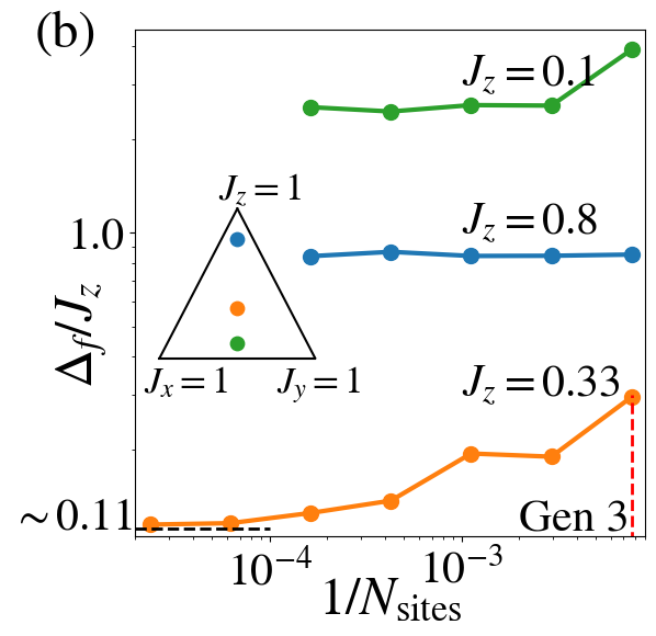
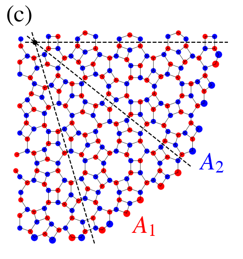
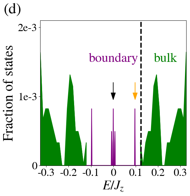
Figure 1: (a) Tri-coordinated quasicrystal with a specific RBG-coloring after generation $\#3$. The original Penrose quasicrystal (black solid lines) divided into two identical triangles using the black dashed lines. The ground state in the canonical flux sector hosts $\pi$ flux on the squares and octagons (shaded plaquettes). The orange dashed line marks one of the five reflection planes, ${\cal{R}}$. (b) Finite size scaling of the bulk gap, $\Delta_{f}/J_{z}$, for three representative points in the parameter space; see inset. The smallest system-size corresponds to generation $\#3$; the extrapolated value ($N_{\rm{sites}}\rightarrow\infty$) of the bulk gap at the isotropic point is $\Delta_{f}/J_{z}\sim 0.11$. (c) Sublattice sites, $A_{1}$ and $A_{2}$, with enlarged boundary dots highlighting the local imbalance (see text). Reflection planes are shown as dashed lines. (d) Low-energy density of states for generation $\#7$ with the lowest-$E$ bulk state (black dashed line) and two representative boundary states (arrows).

Quasicrystalline graph.- Our starting point involves designing a tri-coordinated quasicrystal, which will allow us to label the bonds using a compass-like Ising interaction. We start with the celebrated “Penrose tiling” consisting of two types of rhombii, each of which is made of two identical isosceles triangles — the golden triangle and golden gnomon Penrose (1974). We obtain the tri-coordinated quasicrystal by connecting the centroids of the adjacent triangles si . The Penrose tiling is itself constructed in the usual way by following the standard inflation rules for successive generations Bruijn (1981); Kumar et al. (1986). Associated with every such generation, we obtain the corresponding tri-coordinated quasicrystal; see Fig. 1(a) and si for a visualization of the graph after generation $\#3$. The tri-coordinated quasicrystal is also bipartite, with a local “imbalance” of the two sublattice sites at the edge (sites labeled as $A_{1},~{}A_{2}$; see Fig. 1 (c)), and contains four types of polygons: square, hexagon, octagon, and decagon, respectively. The fraction of each such polygon in the thermodynamic limit is given by si ,

$$(p_{4},p_{6},p_{8},p_{10})=\left(\frac{1}{\tau^{2}},\frac{1}{\tau^{2}},\frac{1}{\tau^{5}},\frac{1}{\tau^{4}}\right),$$ (1)

where $\tau=(\sqrt{5}+1)/2$ is the golden-ratio. The Kitaev model on this graph, as described in detail below, leads to a fully gapped spin liquid in the bulk (Fig. 1(b)).

Kitaev Model.- We introduce a coloring scheme to label each of the three bonds around a vertex as red ($R$), blue ($B$), and green ($G$). Each such vertex is connected to its 3 neighboring sites via an $x$-, $y$-, and $z$-link (corresponding to R, B, G respectively) depending on the direction. These nearest-neighbor bonds represent Kitaev-type spin interactions for $S=1/2$ degrees of freedom on the above quasicrystalline graph. The Hamiltonian is defined as

$$H=\sum_{\langle i,j\rangle_{\mu}}J^{\mu}_{ij}\sigma_{i}^{\mu}\sigma_{j}^{\mu},$$ (2)

where $\sigma_{i}^{\mu}$ $(\mu=x,y,z)$ is a Pauli operator for the spin at site $i=1,\dots,2N$, $\langle i,j\rangle_{\mu}$ is a pair of nearest neighboring sites connected via a $\mu$-link, and $J^{\mu}_{ij}$ are link-dependent couplings. The coloring scheme is not unique, and we choose a specific convention whereby $\{R,B,G\}$ bonds are assigned in a clockwise (counter-clockwise) fashion for vertices belonging to the $A_{1}\ (A_{2})$ sublattice, respectively; see Fig. 1 (a) and si . Our coloring scheme manifestly preserves the reflection symmetries associated with the bond couplings, which will turn out to be crucial for application of Lieb’s flux theorem Lieb (1994); Macris and Nachtergaele (1996). Interestingly, each polygon (plaquette) then consists of only two types of colored bonds, in contrast to the usual honeycomb model.

We define the usual flux operators, $W_{p}\equiv\prod_{\langle i,j\rangle_{\mu}\in\partial P}\sigma_{i}^{\mu}\sigma_{j}^{\mu}$, where $\partial P$ denotes the boundary of the plaquette $p$ oriented in a clockwise fashion. Since $[H,W_{p}]=0$, the eigenstates of the Hamiltonian Eq. 2 can be divided into different flux sectors, $\{w_{p}\}$, where $w_{p}=\pm 1$ represent the flux eigenvalues. Following Kitaev’s presciption Kitaev (2006) we rewrite a spin operator in terms of Majorana fermions $\sigma^{\mu}_{i}=ib^{\mu}_{i}c_{i}$, and define link operators $\hat{u}_{ij}=ib_{i}^{\mu}b_{j}^{\mu}$. Then Eq. 2 can be rewritten as $H_{\hat{u}}=i\sum_{\langle j,k\rangle_{\mu}}J^{\mu}_{jk}\hat{u}_{jk}c_{j}c_{k}$, with $[H_{\hat{u}},\hat{u}_{jk}]=0$, leading to the link operators having conserved eigenvalues. Since the link operators take eigenvalues $u_{jk}=\pm 1$, the problem reduces to $c-$Majorana fermions coupled to the static $Z_{2}$ gauge fields $\{u_{jk}\}$, hopping on the sites of a quasicrystal; however, the lowest energy many-body state need not correspond to all of the $\{u_{jk}\}=1$. For the translationally invariant honeycomb lattice, the ground state is known to be flux-free according to Lieb’s flux theorem Lieb (1994). We next turn to obtaining the ground state flux configuration on the tri-coordinated quasicrystalline graph.

Extended Lieb’s theorem for ground state.- Given that the quasicrystal consists of distinct polygons, it is not obvious a priori whether the ground state can be flux-free, and if not, which polygons host non-zero fluxes. To find the ground state configuration, we perform an extensive sampling of all the distinct flux configurations numerically. We leverage a “generalized” version of Lieb’s theorem Macris and Nachtergaele (1996); Jaffe and Pedrocchi (2014); Chesi et al. (2013) that reduces dramatically the number of samplings required to identify the ground state.

To proceed, we first rewrite the Kitaev quadratic Hamiltonian as,

$$H_{u}=\frac{i}{2}(c_{A_{1}}^{T}\ c_{A_{2}}^{T})\begin{pmatrix}0&M\\ -M^{T}&0\end{pmatrix}\begin{pmatrix}c_{A_{1}}\\ c_{A_{2}}\end{pmatrix},$$ (3)

where $M_{ij}=J^{\mu}_{ij}u_{ij}$, and $c_{A_{1}\>(A_{2})}$ denotes the vector of Majorana operators for the sublattice $A_{1}\>(A_{2})$. We perform a canonical transformation to rewrite Eq. 3 as $H_{u}=\sum_{m=1}^{N}\varepsilon_{m}(2a^{\dagger}_{m}a_{m}-1)$ in terms of complex fermions, $a_{m},~{}a_{m}^{\dagger}$, where $\varepsilon_{m}$ are non-negative eigenvalues of $M$. The cost of adopting the above representation is an enlarged Hilbert space; we project out the unphysical states based on the parity of the fermionic eigenmodes, $\prod_{m}(1-2n_{m})$, where $n_{m}=a^{\dagger}_{m}a_{m}$ si ; Yao et al. (2009); Pedrocchi et al. (2011).

Consider a generic two-dimensional bipartite graph $\Lambda$, with a nearest-neighbor Hamiltonian defined for Majorana fermions, $H=\sum_{x,y\in\Lambda}iJ_{xy}u_{xy}c_{x}c_{y}$, where $J_{xy}\geq 0$ and $u_{xy}=\pm 1$. The flux of a given plaquette $W_{p}$ can be written as $W_{p}=\prod_{(ij)\in\partial p}u_{ij}$, where $i$ ($j$) belongs to the $A_{1}$ ($A_{2}$) sublattices of the boundary of a plaquette $p$. At half-filling (of the complex fermion representation), flux sectors minimizing the ground state energy satisfy the following properties Chesi et al. (2013): (i) the plaquettes intersecting ${\cal{R}}$ have a canonical flux $W_{p}=-(-1)^{L/2}$ where $L$ is the number of edges of the plaquette, and (ii) the remaining plaquettes have the same flux as their reflected plaquette, i.e. $W_{p}=W_{r(p)}$.

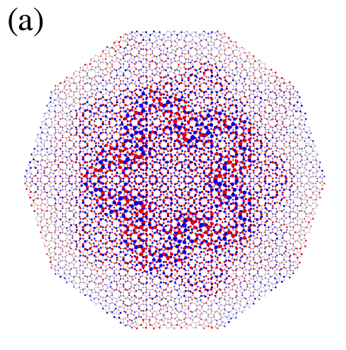
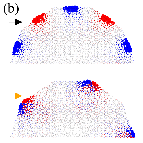
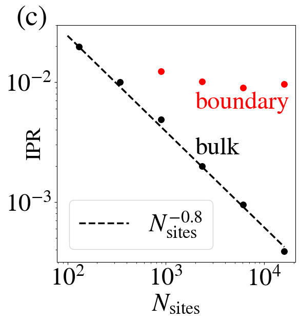
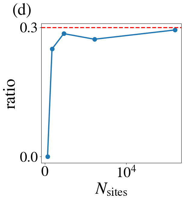
Figure 2: Distribution of the fermionic wave function for (a) the lowest-$E$ bulk state, and (b) two representative boundary states associated with the marked arrows in Fig. 1(d), respectively. The blob size denotes the probability of finding the state at that site, and the color (red/blue) represents the sublattice. (c) Finite size scaling of the IPR. The bulk IPR is computed for the lowest-energy bulk state, while the boundary IPR is obtained by averaging over all boundary states. (d) The ratio between the number of boundary states and local imbalance, $\Delta N$, as a function of system size.

For our quasicrystal, there are five reflection planes bisecting the edges of the central decagon at right angles; see Fig. 1(a). The flux associated with the plaquettes intersecting ${\cal{R}}$ are fixed by property (i). For the remaining plaquettes, we divide the entire system into ten reflection-symmetric sectors. Within each sector involving $N_{p}$ plaquettes not intersected by the ${\cal{R}}$, we can identify a total of $2^{N_{p}}$ distinct flux sectors. We find the configuration with the minimum ground state energy, $E_{\textnormal{GS}}$, after sampling over all distinct flux configurations, keeping reflection-symmetric $\{u_{ij}\}$ and constraining to the physical Hilbert space with $\sum_{m}n_{m}=0$. We observe that $E_{\textnormal{GS}}$ is minimized when every plaquette has canonical flux (see definition above and Fig. 1 (a)); we dub this the canonical flux sector. By varying the anisotropy associated with the Kitaev exchange (i.e.  $J^{z}/J,J^{x}=J^{y}=J$) we have confirmed that the canonical flux sector continues to remain the ground state si . We have performed the numerical flux samplings up to generation $\#4$ (where the total number of sites$=340$) and confirmed that the above result continues to remain valid. For higher generations, the sampling procedure becomes increasingly computationally intense, and so we assume that the ground state will continue to conform to the canonical flux sector. We next turn to the nature of the excitations above the canonical ground state flux sector.

Fermionic excitations.- The Hamiltonian defined on any finite system reveals an interesting excitation spectrum; see, for instance, Fig. 1(d) for the density of states (DOS) at the isotropic point. While a naive interpretation might lead us to conclude the existence of a gapless phase (with $E=0$) over a broad range of parameters, a careful analysis reveals that the bulk and boundary states need to be disentangled first in order to obtain the actual phase diagram.

We first use the local DOS as a diagnostic. If the position of the peak of $|\psi_{n}(r)|^{2}$ is located deep in the bulk (near the boundary), where $\psi_{n}(r)$ is the wave function of the $n$-th state at site $r$, the state can be identified as a bulk (boundary) state; see si for details. We define the bulk gap $\Delta_{f}$ as the minimum energy eigenvalue of all the bulk states. Interestingly, we find that the fermionic spectrum is gapped regardless of the choice of couplings, in stark contrast with the translationally invariant version of the original model on the honeycomb lattice.

To demonstrate the gapped bulk spectrum, we perform finite-size scaling with a few representative points with different $J_{z}$, keeping $J_{x}=J_{y}$ and $\sum_{\mu}J_{\mu}=1$ (Fig. 1(b)). In one anisotropic limit $J_{z}\rightarrow 0$, our quasicrystal is decoupled into a set of disconnected polygons with only $x$ and $y-$links; $\Delta_{f}$ is thus determined by the spectrum of the largest polygon — a decagon. Note that the same limit describes a set of decoupled one-dimensional chains for the honeycomb Kitaev model. In the other limit of $J_{z}\rightarrow 1$, the QC is divided into decoupled dimers connected by $z-$links, and $\Delta_{f}$ is determined by the spectrum of a single dimer; this is also true for the honeycomb Kitaev model. These energy scales in the two anisotropic limits remain finite with increasing number of generations, and the spectrum is gapped. At the isotropic point, we have carried out a study with increasing system size and find that $\Delta_{f}$ converges to a small but finite value $\Delta_{f}/J_{z}\sim 0.11$; see Fig. 1(b). Note that the fermions in the canonical flux sector are subject to an effective inhomogeneous emergent magnetic field through specific plaquettes. As this magnetic field is switched off, the system enters the flux-free sector, but with a greater energy, where we find the spectrum is gapless with $\Delta_{f}$ scaling as $\sim N_{\textnormal{sites}}^{-\alpha}$ with $\alpha\approx 0.6$, where $N_{\textnormal{sites}}$ denotes the total number of sites si . This suggests that the fermionic gap is likely tied to the Hofstadter butterfly problem on the quasicrystal due to the inhomogeneous emergent $Z_{2}$ fluxes of the ground state Fuchs and Vidal (2016); connecting this to the gap-labeling conjecture for quasicrystals Johnson and Moser (1982); Bellissard et al. (2005); Benameur and Oyono-Oyono (2007) remains an interesting open problem. We have also studied the effect of a perturbative magnetic field along the $[1,1,1]$ direction, which drives a gap-closing quantum phase transition to a chiral spin liquid on the quasicrystal si .

Let us now comment on the spatial distribution of the bulk and boundary states tied to specific energies. We plot the wavefunction distribution for the lowest energy bulk state (Fig. 1(d)) in Fig. 2(a). It is evident that the wavefunction has support over a large fraction of the sites and exhibits a (quasi-)delocalized behavior, which will be clarified further when we introduce the inverse participation ratio (IPR) as a diagnostic. The boundary states associated with two different energies (Fig. 1(d)) are clearly localized along the edge, and interestingly, have a strong sub-lattice dependence (Fig. 2(b)). The boundary states are strongly affected by the local topology Sutherland (1986); Day-Roberts et al. (2020) and favor the majority sublattice site along the boundary within each region (see Fig. 1 (c)). It is known that such local imbalance between the population of two sublattices can result in localized zero-energy states Day-Roberts et al. (2020). We revisit this point below, after highlighting the contrast between the (de-)localization properties associated with the bulk vs. boundary states.

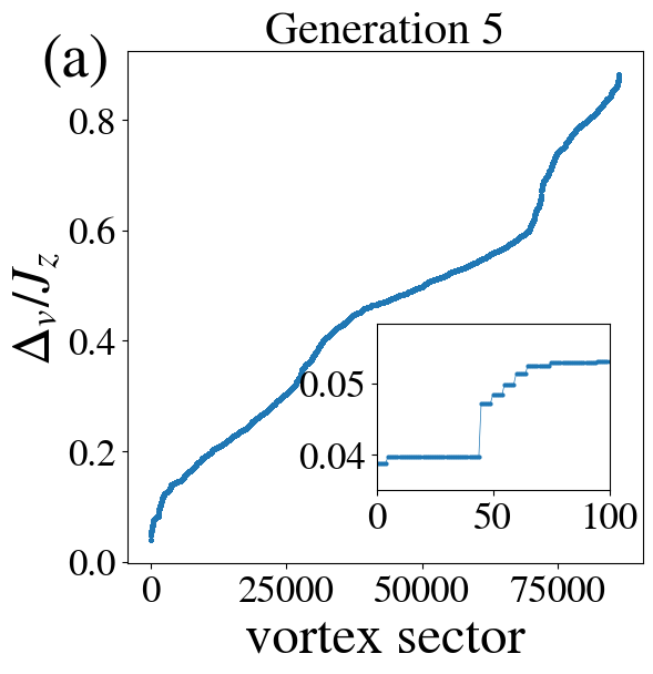
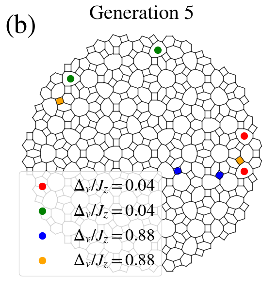
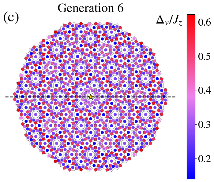
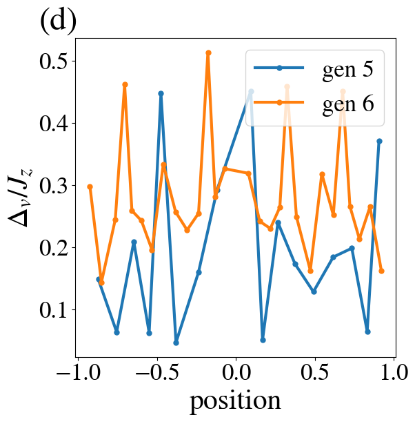
Figure 3: (a) The vortex-pair excitation energy at the isotropic point for generation $\#5$. Inset: Enlarged plot for the first few plateaus. (b) The two lowest (red and green) and highest (blue and orange) energy vortex-pair configurations, respectively. Note that vortices carry an $n\pi$ flux (mod $2\pi$) for the polygon with length $n$. (c) The map of the vortex energy when one vortex is fixed at the center (denoted ‘$\star$’). (d) Position-dependence of the vortex energy along the horizontal dashed line shown in (c). The position is rescaled by the radius of the system.

Let us introduce the IPR as

$$\textnormal{IPR}_{n}=\sum_{r=1}^{N_{\textnormal{sites}}}|\psi_{n}(r)|^{4}.$$ (4)

Recall that a typical extended state satisfies an IPR scaling as $\sim N_{\textnormal{sites}}^{-1}$, while a typical localized state has a system-size independent IPR. In Fig. 2(c), we present the finite size scaling of the IPR for the lowest-energy bulk state and the IPR averaged over all the boundary states. As we noted in Fig. 2(a), we indeed find that the bulk states are delocalized over a finite fraction of the system with an IPR scaling as $\sim N_{\textnormal{sites}}^{-0.8}$. The slight deviation from the typical extended behavior in crystalline systems with translational symmetry is controlled by the unconventional distribution of sites on the quasicrystal. The exponent is likely tied to the fractal dimension of the corresponding state Halsey et al. (1986); Kohmoto et al. (1987b); Roche et al. (1997). The boundary states, on the other hand, are strongly localized along the edges leading to a nearly size-independent IPR. To quantitatively study the relation between the boundary states and the local imbalance, we introduce $\Delta N=\sum_{\textnormal{regions}}|N_{A_{1}}-N_{A_{2}}|$, where $N_{A_{1},A_{2}}$ represents the number of sites belonging to each sublattice in each of the 10 regions partitioned by the reflection planes (Fig. 1(c)) Day-Roberts et al. (2020). In Fig. 2(d), we plot the ratio between the number of boundary states and $\Delta N$ with increasing system size. For generations $\#4$ $(N_{\textnormal{sites}}\leq 340)$ and higher, the ratio converges to a finite value $\sim 0.3$ (red dashed line), demonstrating the close connection between the boundary states and the local imbalance. The zero-energy states are fragile against perturbations that do not preserve the local imbalance. For the analysis of $E=0$ states, the $2-$coordinated sites are paired up by infinitesimal couplings to preserve the original boundary condition. Connecting these sites via a non-zero coupling eventually gets rid of these $E=0$ states.

To illustrate the origin of the connection between local imbalance and zero-energy modes, consider a bipartite lattice with nearest-neighbor hoppings and a block-diagonal Hamiltonian, $H=\begin{pmatrix}0&G\\ G^{T}&0\end{pmatrix}$. Due to the imbalance (e.g. without any loss of generality, more $A_{1}$ sites compared to $A_{2}$), the number of rows and columns in $G$ are different, leading to some eigenstates with zero eigenvalue. The corresponding $E=0$ states are then localized on the majority sublattice $(A_{1})$. A prominent example of this phenomenon arises on the Penrose quasicrystal Kohmoto and Sutherland (1986); Arai et al. (1988), which hosts $E=0$ states throughout the bulk since the system can be partitioned into decoupled sectors by “membranes” that preclude any zero-energy states Flicker et al. (2020); Day-Roberts et al. (2020). In contrast, for our tri-coordinated quasicrystal, only the boundary exhibits a local imbalance leading to localization along the edge. We have also obtained boundary states with a small non-zero energy, manifest in the intermediate peaks over a finite range of energy $0<E<\Delta_{f}$ (Fig. 1(d)). These states remain distributed near the boundary, but are not strictly localized.

Vortex excitations.- Turning our attention now to the vortex-like excitations, let us consider a pair of vortices on top of the canonical ground-state flux sector at the isotropic point. In the absence of crystalline translational symmetry, the vortex pair energy can be strongly dependent on their locations. In Fig. 3(a), we plot the complete set of vortex pair energy, $\Delta_{v}$, for the vortices placed at any two polygons for generation $\#5$. The plot shows multiple plateaus (see inset), which represents the number of geometrically equivalent vortex configurations. In Fig. 3(b), we display the vortex pair configurations associated with the two lowest and highest energies, respectively. Interestingly, the lowest energy vortex pair excitations correspond to the vortices located in a reflection-symmetric fashion, suggesting that a version of Lieb’s flux theorem might still have some bearing on these low-energy excitations. Moreover, as already indicated above, in the absence of crystalline symmetries, $\Delta_{v}$ is not a simple monotonous function of the spatial separation between the vortices, but instead depends both on the type of polygon and their positions. To illustrate this, we fix one vortex at the center of the quasicrystalline graph and map out the $\Delta_{v}$ tied to placing the other vortex at any other location on the graph; see Fig. 3(c). The energetic hierarchy indicates that $\Delta_{v}$ tends to be larger when a vortex is located on the smaller polygons. A scan of $\Delta_{v}$ along a high-symmetry cut (black dashed line in Fig. 3(c)) is shown in Fig. 3(d). The vortex pairs are deconfined as the energy cost associated with moving them apart does not continue to grow with increasing separation.

Outlook.- This work demonstrates the complexity associated with the interplay of fractionalization, entanglement and (de-)localization in quasicrystalline graphs. While serving as an important proof-of-concept demonstration of the novel aspects of frustrated spin models in quasicrystals, the advent of programmable Rydberg quantum simulators and interesting dynamical protocols Kalinowski et al. (2023) can potentially help realize such phases in the laboratory in the not too distant future.

Going beyond the classic Kitaev model construction, other exciting avenues for future work include extending the model Yao and Kivelson (2007); Yao and Lee (2011) on the same (or different Keskiner et al. (2023); Wu et al. (2009)) quasicrystals, studying variants of the Kitaev-Kondo model Tsvelik and Coleman (2022) inspired by intriguing experiments in metallic quasicrystals Andrade et al. (2015), and addressing the properties of a few doped particles on top of the spin liquid ground state Halász et al. (2014). Developing a field-theoretic understanding of these phases while incorporating their quasicrystalline character from the outset also remains an interesting open problem.

Acknowledgements.- We thank Daniel Arovas, Junmo Jeon and SungBin Lee for insightful discussions, and Omri Lesser for a critical reading of an earlier version of this manuscript. SK, DM and DC are supported in part by a New Frontier Grant awarded by the College of Arts and Sciences at Cornell University and by a Sloan research fellowship from the Alfred P. Sloan foundation to DC. DM is also supported by a Bethe postdoctoral fellowship at Cornell University. DC acknowledges the support provided by the Aspen Center for Physics, which is supported by National Science Foundation grant PHY-1607611. AA acknowledges support from IITK Initiation Grant (IITK/PHY/2022010). AA acknowledges engaging discussions at the Indo-French meeting “Novel Phases of Matter in Frustrated Magnets” at Bordeaux, France.

Supplementary material for “Quasicrystalline Spin Liquids”

I Additional details on the construction of the tri-coordinated quasicrystal

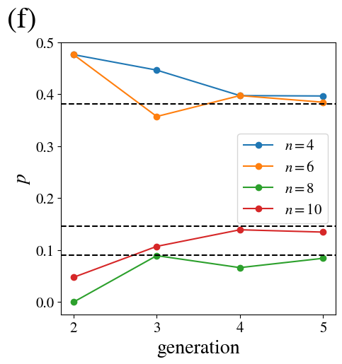
Supplemental Figure S1: Construction of our tri-coordinated quasicrystal starting from (a) generation $\#1$ up to (c) generation $\#3$. The underlying Penrose QCs are marked by black solid and dashed lines as with the main text. (d) Illustration of inflation rules for the Penrose QC. Upon inflation, each rhombus is divided into smaller rhombi. The solid lines mark the boundary of rhombi, while the dashed lines serve as a guide to eye for triangulation. (e) Illustration of the 8 types of vertices of the Penrose QC. (f) The fraction of each polygon $(n=4,6,8,10)$ with increasing generation. The black dashed lines mark the asymptotic expected behavior of $\tau^{-2},\tau^{-4},\tau^{-5}$ ($\tau\equiv$golden-ratio), respectively, from top to bottom.

In Fig. S1(a)-(c), we present the configuration of the tri-coordinated quasicrystal up to generation $\#3$ with our specific choice of the 3-coloring convention (see main text). The tri-coordinated quasicrystal can be viewed as the dual lattice of a triangulated Penrose quasicrystal of the same generation. We note an interesting even-odd effect tied to the configurations: The central decagon in the odd-generations is surrounded by 5 squares and 5 hexagons, while the central decagon in the even-generations is surrounded by 10 hexagons. This even-odd effect manifests in the finite size scaling of the bulk gap, e.g. see Fig. S4.

From the inflation properties of the Penrose QC (see Fig. S1(d)), we can obtain the fraction of each polygon in the thermodynamic limit. The Penrose QC consists of 8 types of vertices with different connectivities, which are denoted as $D,J,Q,K,S3,S4,S$ and $S5$; see Fig. S1(e). Let $\bm{n}_{k}$ denote an eight-dimensional vector for the number of each type of vertex for generation $\#k$. Upon inflation, two consecutive number vectors are related by a transfer matrix, i.e. $\bm{n}_{k+1}=M\bm{n}_{k}$ De Bruijn (1981); Kumar et al. (1986). The fractions of each type of vertex in the thermodynamic limit are determined by the largest eigenvalue of the matrix, $\tau^{2}$, where $\tau=(\sqrt{5}+1)/2$ is the golden ratio. In the thermodynamic limit, the fraction of each type is given by $\left(\frac{1}{\tau^{2}},\frac{1}{\tau^{3}},\frac{1}{\tau^{4}},\frac{1}{\tau^{5}},\frac{1}{\tau^{6}},\frac{1}{\tau^{7}},\frac{1}{\tau^{4}(1+\tau^{2})},\frac{1}{\tau^{6}(1+\tau^{2})}\right)$. We can readily find the correspondence between the vertices and the polygons as follows: $D\leftrightarrow 4,(Q,J)\leftrightarrow 6,K\leftrightarrow 8$, and $(S3,S4,S,S5)\leftrightarrow 10$. We thus obtain the fraction of each polygon in the thermodynamic limit as

$$(p_{4},p_{6},p_{8},p_{10})=\left(\frac{1}{\tau^{2}},\frac{1}{\tau^{2}},\frac{1}{\tau^{5}},\frac{1}{\tau^{4}}\right).$$ (I.1)

In Fig. S1 (f), we present the fraction of each polygon as a function of generation. Each fraction converges to irrational values, $\tau^{-x}$ $(x=2,4,5)$, marked by black dashed lines.

II Projection onto the physical subspace

In this section, we provide details on how to project out unphysical states, based on the derivation in Pedrocchi et al. (2011). We consider a local operator, $D_{i}=-i\sigma_{i}^{x}\sigma_{i}^{y}\sigma_{i}^{z}=1$, which serves as the identity operator in the original physical subspace. We can rewrite the operator in terms of the Majorana operators as $D_{i}=b^{x}_{i}b^{y}_{i}b^{z}_{i}c_{i}$, which has eigenvalues $\pm 1$. The projection operator onto the physical subspace is thus given by

$$P=\prod_{i=1}^{2N}\left(\frac{1+D_{i}}{2}\right)=S\cdot\left(\frac{1+\prod_{i=1}^{2N}D_{i}}{2}\right)\equiv S\cdot P_{0},$$ (II.2)

where $S$ symmetrizes over all gauge equivalent $\{u_{ij}\}$ sectors and $P_{0}$ projects out unphysical states.

Our goal is to express $P_{0}$ in terms of the variables that are used to label a state: the field configuration $\{u_{ij}\}$ and the fermion occupation $\{n_{m}\}$. We start by rewriting $D\equiv\prod_{i=1}^{2N}D_{i}$ as

$$D=\prod_{i=1}^{2N}c_{i}\prod_{i=1}^{2N}b_{i}^{x}\prod_{i=1}^{2N}b_{i}^{y}\prod_{i=1}^{2N}b_{i}^{z}\equiv(-1)^{\theta}\prod_{i=1}^{2N}c_{i}\cdot\prod_{\mu=x,y,z}\left(\prod_{\langle ij\rangle_{\mu}}b^{\mu}_{i}b^{\mu}_{j}\right)=(-1)^{\theta}\prod_{i=1}^{2N}c_{i}\cdot\prod_{\mu=x,y,z}\left(\prod_{\langle ij\rangle_{\mu}}-iu_{ij}\right),$$ (II.3)

where $(-1)^{\theta}=\pm 1$ arises from the reordering of the $b_{i}^{\mu}$ operators, which depends on the choice of lattice labelings. For numerical calculations, we have chosen a labeling such that $i\leq N$ ($N+1\leq i$) belongs to the sublattice $A_{1}$ ($A_{2}$).

To deal with $\prod_{i=1}^{2N}c_{i}$, we revisit the canonical transformation of the Majorana Hamiltonian. We consider a singular-value decomposition, $M=USV^{T}$, where $U$ and $V$ are $N\times N$ orthogonal matrices and $S=\textnormal{diag}(\varepsilon_{1},\dots,\varepsilon_{N})$ with $\varepsilon_{m}\geq 0$. We rewrite the Hamiltonian as

$$H_{u}=\frac{i}{2}(c_{A_{1}}^{T}\ c_{A_{2}}^{T})\begin{pmatrix}0&M\\ -M^{T}&0\end{pmatrix}\begin{pmatrix}c_{A_{1}}\\ c_{A_{2}}\end{pmatrix}=i\sum_{m=1}^{N}\varepsilon_{m}c_{A_{1},m}^{\prime}c_{A_{2}.m}^{\prime}=\sum_{m=1}^{N}\varepsilon_{m}(2a^{\dagger}_{m}a_{m}-1),$$ (II.4)

where we have introduced new Majorana fermions, $(c_{A_{1},1}^{\prime},\dots,c_{A_{1},N}^{\prime})=(c_{A_{1},1},\dots,c_{A_{1},N})U$ and $(c_{A_{2},1}^{\prime},\dots,c_{A_{2},N}^{\prime})=(c_{A_{2},1},\dots,c_{A_{2},N})V$. The last equality in Eq. II.4 is followed by the canonical transformation $a_{m}\equiv(c_{A_{1},m}^{\prime}+ic_{A_{2},m}^{\prime})/2$ and $a_{m}^{\dagger}\equiv(c_{A_{1},m}^{\prime}-ic_{A_{2},m}^{\prime})/2$. We then obtain

$$\prod_{i=1}^{2N}c_{i}=\prod_{m=1}^{N}c_{A_{1},m}\prod_{m=1}^{N}c_{A_{2},m}=\left(\textnormal{det}(U)\prod_{m=1}^{N}c_{A_{1},m}^{\prime}\right)\left(\textnormal{det}(V)\prod_{i=m}^{N}c_{A_{2},m}^{\prime}\right)=\textnormal{det}(U)\textnormal{det}(V)(-1)^{\frac{N(N-1)}{2}}\prod_{m=1}^{N}\left(c_{A_{1},m}^{\prime}c_{A_{2},m}^{\prime}\right).$$

Noting that $c_{A_{1},m}^{\prime}c_{A_{2},m}^{\prime}=i(1-2n_{m})$, we finally obtain

$$D=(-1)^{\theta}\textnormal{det}(U)\textnormal{det}(V)(-1)^{\frac{N(N-1)}{2}}\cdot i^{N}\prod_{m=1}^{N}(1-2n_{m})\cdot\left(\prod_{\langle ij\rangle_{\mu}}-iu_{ij}\right).$$ (II.6)

Eq. II.6 can be used to determine $\{u_{ij}\}$ and $\{n_{m}\}$ for the physical ground state satisfying $P_{0}=1$. For a given flux sector, a naïve ground state energy is $E_{gs}^{0}=-\sum_{m=1}^{N}\varepsilon_{m}$, which amounts to the energy of the half-filled particle-hole symmetric spectrum, $(-\varepsilon_{N},\dots,\varepsilon_{N})$. If $\{u_{ij}\}$ from the canonical flux sector is physical when $\sum_{m=1}^{N}n_{m}=0$, then such a state is the true ground state according to the Lieb’s theorem. If not, however, we have to change the parity of the fermion occupation by 1, departing from the half-filling. Thus, the flux sampling must extend to the ones violating the two basic assumptions (described in the main text) of the Lieb’s theorem. For the flux sampling, one can come up with an appropriate spanning tree that bisects links of plaquettes (not intersected by the reflection planes) $N_{p}$ times. Each flux sector corresponds to a set of flipped links on the spanning tree. The resulting gauge choice for the canonical flux sector is, for instance, shown in Fig. S3.

III Additional results for flux sampling

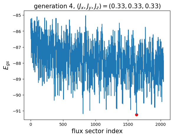
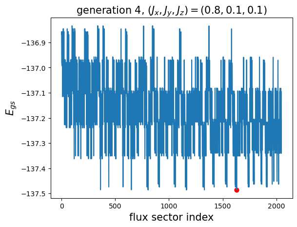
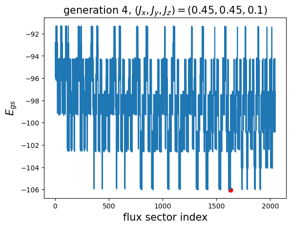
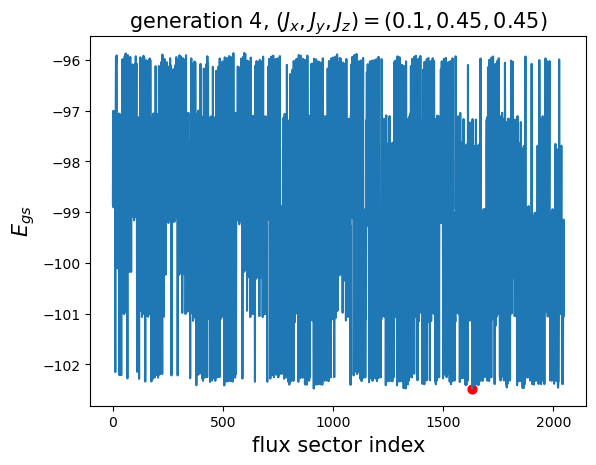
Supplemental Figure S2: Flux sampling for generation $\#4$ at four representative points in the phase diagram. The red-circle denotes the canonical flux-sector associated with the ground-state.

In Fig. S2, we present additional flux sampling results for generation $\#4$ at a few representative points in the phase diagram. The canonical flux sector (red circle) remains the ground state flux sector regardless of the choice of $\{J_{\mu}\}$. We show in Fig. S3 the $Z_{2}$ field configuration for the ground state (canonical) flux sector at the isotropic point. Here the shaded red bond shows the links where $u_{ij}=-1$ in our gauge choice.

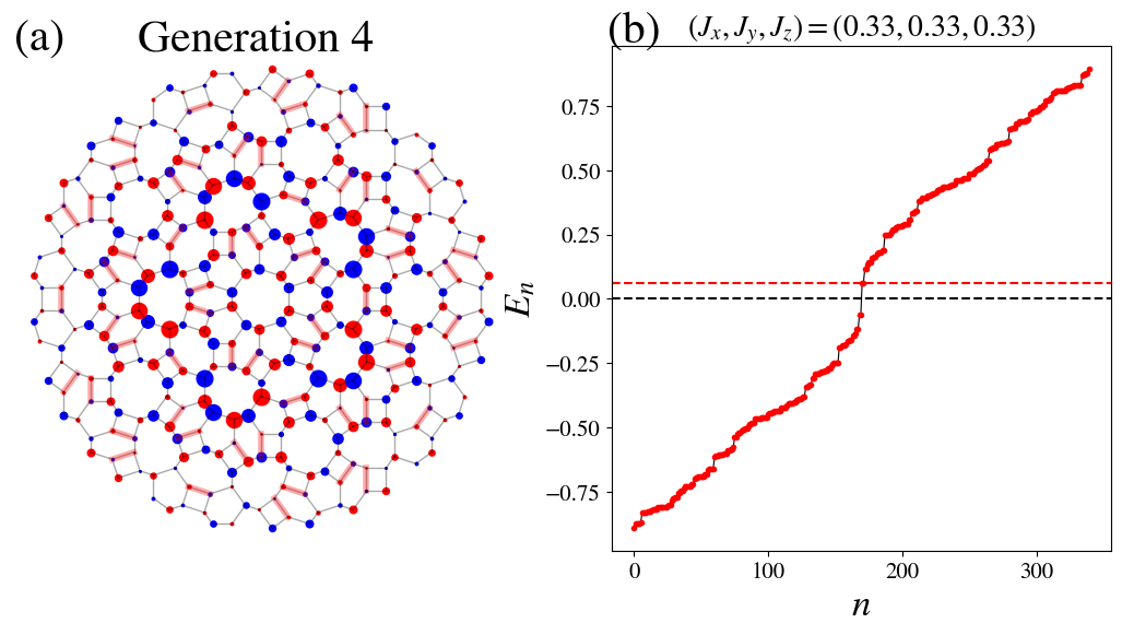
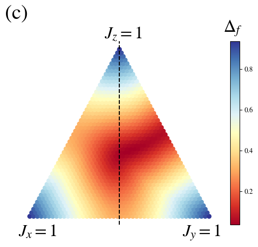
Supplemental Figure S3: (a) Ground state $Z_{2}$ field configuration and distribution of lowest-energy bulk fermionic excitations. The red (black) lines denote bonds with $u_{ij}=-1\ (+1)$. The size of a blob quantifies the probability of finding the lowest energy fermionic excitations. (b) The fermionic spectrum with the red dashed line being the lowest-energy bulk state. (c) Bulk fermionic gap $\Delta_{f}$ on the plane $\sum_{\mu}J_{\mu}=1$ in the parameter space. The three representative set of parameters for the analysis of the bulk gap are located on the vertical dashed line.

Supplemental Figure S4: Results for the higher energy flux-free sector. (a) The wave function distribution for the lowest-$E$ bulk state. (b) Fermionic spectrum. (c) Finite size scaling of the bulk gap.

We show in Fig. S4 results for the flux-free sector, which has higher energy than the canonical flux sector. In this case, the system at the isotropic point becomes gapless with $\Delta_{f}$ scaling as $\sim N_{\textnormal{sites}}^{-0.6}$. We note an even-odd effect manifest in the finite-size scaling of $\Delta_{f}$.

IV LDOS as a function of position

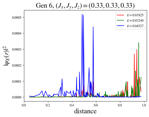
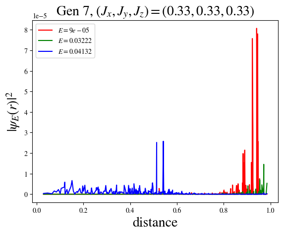
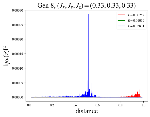
Supplemental Figure S5: Local DOS as a function of distance from the center. The distance is rescaled by the radius of the system.

To identify true bulk excitations, we study the local density of states (LDOS) of low-energy excitations. For a given state with energy $E$, we can compute the amplitude of the state localized at site $i$, $\psi_{E}(i)$. Then we can obtain a histogram of $|\psi_{E}(r)|^{2}$ for all sites $i=1,\cdots,N_{sites}$ as a function of distance $r$ measured from the origin. In Fig. S5, we present the histogram for generations $\#$6, 7, 8. The red and green curves are typical boundary states. The blue curves are the lowest-energy states for which the peaks are located deep in the bulk, and thus they can be identified as lowest-energy bulk states. Distance represents the atomic position rescaled by the radius of the system.

V Spectral functions of fermionic excitations in reciprocal space

Supplemental Figure S6: Energy-resolved spectral function in reciprocal space at four representative energy values (for generation $\#4$ at the isotropic point). $\langle a\rangle$ denotes an average atomic constant of the QC.

For a better understanding of the fermionic spectrum, we study the spectral function in reciprocal space. While the quasicrystal lacks a Brillouin zone associated with translational symmetry, we can still compute a spectral function defined as

$$A(\omega,\bm{k}) = -\frac{1}{\pi}\textnormal{Im}G^{R}(\omega,\bm{k})$$ (V.7)

$$= -\frac{1}{\pi}\textnormal{Im}\sum_{\bm{r}_{1},\bm{r}_{2}}\psi_{\bm{k}}(\bm{r}_{1})^{*}G^{R}(\omega,\bm{r}_{1},\bm{r}_{2})\psi_{\bm{k}}(\bm{r}_{2}),$$

where $G^{R}(\omega,\bm{r}_{1},\bm{r}_{2})$ is the retarded Green’s function and $\psi_{\bm{k}}(\bm{r})=\frac{1}{\sqrt{N}}e^{i\bm{k}\cdot\bm{r}}$ is the plane wave function. In Fig. S6, we present energy-resolved spectral functions in reciprocal space at four representative energy values across the spectrum at the isotropic point for generation $\#4$. The spectral function displays salient differences from the counterpart on the honeycomb model. First, the spectral functions exhibit a clear 5-fold rotational symmetry tied to the underlying symmetry of the quasicrystal. Moreover, there are 10 peaks of the spectral function at finite energy $\omega>\Delta_{f}$, around which the Dirac-like features are absent.

VI Chiral spin liquid

Supplemental Figure S7: Chiral spin liquid obtained by applying an external magnetic field $(\kappa\sim\frac{h_{x}h_{y}h_{z}}{J^{2}}\ll J)$ at the isotropic point. (a) Gap-closing transition as a function of field. (b) Boundary state distribution, where the red bonds have $u_{ij}=-1$ in our gauge choice. (c) Fermionic spectrum of the CSL phase (obtained for generation $\#$4).

Similar to the honeycomb model, a chiral spin liquid (CSL) can be realized by applying a small magnetic field along the $[1,1,1]$ direction to the system near the isotropic point. An important difference of the quasicrystalline model is that the field-induced transition to the CSL is now accompanied by gap closing, as shown in Fig. S7 (a). $\kappa\sim h_{x}h_{y}h_{z}/J^{2}$ denotes a perturbative external magnetic field. A chiral boundary mode is manifest in Fig. S7 (b-c).

References

- Ranganathan and Chattopadhyay (1991) S. t. Ranganathan and K. Chattopadhyay, “Quasicrystals,” Annual Review of Materials Science 21, 437 (1991).
- Levine and Steinhardt (1984) D. Levine and P. J. Steinhardt, “Quasicrystals: A new class of ordered structures,” Phys. Rev. Lett. 53, 2477 (1984).
- Goldman and Kelton (1993) A. I. Goldman and R. F. Kelton, “Quasicrystals and crystalline approximants,” Rev. Mod. Phys. 65, 213 (1993).
- Goldman and Widom (1991) A. Goldman and M. Widom, “Quasicrystal structure and properties,” Annual Review of Physical Chemistry 42, 685 (1991).
- Bindi et al. (2009) L. Bindi, P. J. Steinhardt, N. Yao, and P. J. Lu, “Natural quasicrystals,” Science 324, 1306 (2009).
- Uri et al. (2023) A. Uri, S. C. de la Barrera, M. T. Randeria, D. Rodan-Legrain, T. Devakul, P. J. D. Crowley, N. Paul, K. Watanabe, T. Taniguchi, R. Lifshitz, L. Fu, R. C. Ashoori, and P. Jarillo-Herrero, “Superconductivity and strong interactions in a tunable moiré quasicrystal,” Nature 620, 762 (2023).
- Ahn et al. (2018) S. J. Ahn, P. Moon, T.-H. Kim, H.-W. Kim, H.-C. Shin, E. H. Kim, H. W. Cha, S.-J. Kahng, P. Kim, M. Koshino, et al., “Dirac electrons in a dodecagonal graphene quasicrystal,” Science 361, 782 (2018).
- Pezzini et al. (2020) S. Pezzini, V. Miseikis, G. Piccinini, S. Forti, S. Pace, R. Engelke, F. Rossella, K. Watanabe, T. Taniguchi, P. Kim, et al., “30-twisted bilayer graphene quasicrystals from chemical vapor deposition,” Nano letters 20, 3313 (2020).
- Deng et al. (2020) B. Deng, B. Wang, N. Li, R. Li, Y. Wang, J. Tang, Q. Fu, Z. Tian, P. Gao, J. Xue, and H. Peng, “Interlayer decoupling in 30° twisted bilayer graphene quasicrystal,” ACS Nano 14, 1656 (2020).
- Lv et al. (2021) B. Lv, R. Chen, R. Li, C. Guan, B. Zhou, G. Dong, C. Zhao, Y. Li, Y. Wang, H. Tao, et al., “Realization of quasicrystalline quadrupole topological insulators in electrical circuits,” Communications Physics 4, 108 (2021).
- Varjas et al. (2019) D. Varjas, A. Lau, K. Pöyhönen, A. R. Akhmerov, D. I. Pikulin, and I. C. Fulga, “Topological phases without crystalline counterparts,” Phys. Rev. Lett. 123, 196401 (2019).
- Else et al. (2021) D. V. Else, S.-J. Huang, A. Prem, and A. Gromov, “Quantum many-body topology of quasicrystals,” Phys. Rev. X 11, 041051 (2021).
- Fan and Huang (2022) J. Fan and H. Huang, “Topological states in quasicrystals,” Frontiers of Physics 17, 13203 (2022).
- Longhi (2019) S. Longhi, “Topological phase transition in non-hermitian quasicrystals,” Phys. Rev. Lett. 122, 237601 (2019).
- Cain et al. (2020) J. D. Cain, A. Azizi, M. Conrad, S. M. Griffin, and A. Zettl, “Layer-dependent topological phase in a two-dimensional quasicrystal and approximant,” Proceedings of the National Academy of Sciences 117, 26135 (2020).
- Jeon et al. (2022) J. Jeon, M. J. Park, and S. Lee, “Length scale formation in the landau levels of quasicrystals,” Phys. Rev. B 105, 045146 (2022).
- Kohmoto et al. (1987a) M. Kohmoto, B. Sutherland, and C. Tang, “Critical wave functions and a cantor-set spectrum of a one-dimensional quasicrystal model,” Phys. Rev. B 35, 1020 (1987a).
- Kohmoto and Banavar (1986) M. Kohmoto and J. R. Banavar, “Quasiperiodic lattice: Electronic properties, phonon properties, and diffusion,” Phys. Rev. B 34, 563 (1986).
- Kohmoto and Sutherland (1986) M. Kohmoto and B. Sutherland, “Electronic states on a penrose lattice,” Phys. Rev. Lett. 56, 2740 (1986).
- Arai et al. (1988) M. Arai, T. Tokihiro, T. Fujiwara, and M. Kohmoto, “Strictly localized states on a two-dimensional penrose lattice,” Phys. Rev. B 38, 1621 (1988).
- Kohmoto (1987) M. Kohmoto, “Electronic states of quasiperiodic systems: Fibonacci and penrose lattices,” International Journal of Modern Physics B 1, 31 (1987).
- Kim et al. (2023) S. Kim, A. Agarwala, and D. Chowdhury, “Fractionalization and topology in amorphous electronic solids,” Phys. Rev. Lett. 130, 026202 (2023).
- Grushin and Repellin (2023) A. G. Grushin and C. Repellin, “Amorphous and polycrystalline routes toward a chiral spin liquid,” Phys. Rev. Lett. 130, 186702 (2023).
- Cassella et al. (2023) G. Cassella, P. d’Ornellas, T. Hodson, W. M. H. Natori, and J. Knolle, “An exact chiral amorphous spin liquid,” Nature Communications 14 (2023), 10.1038/s41467-023-42105-9.
- Kitaev (2006) A. Kitaev, “Anyons in an exactly solved model and beyond,” Annals of Physics 321, 2 (2006).
- Hermanns et al. (2018) M. Hermanns, I. Kimchi, and J. Knolle, “Physics of the kitaev model: Fractionalization, dynamic correlations, and material connections,” Annual Review of Condensed Matter Physics 9, 17 (2018).
- Trebst and Hickey (2022) S. Trebst and C. Hickey, “Kitaev materials,” Physics Reports 950, 1 (2022).
- Willans et al. (2010) A. J. Willans, J. T. Chalker, and R. Moessner, “Disorder in a quantum spin liquid: Flux binding and local moment formation,” Phys. Rev. Lett. 104, 237203 (2010).
- Sreejith et al. (2016) G. J. Sreejith, S. Bhattacharjee, and R. Moessner, “Vacancies in kitaev quantum spin liquids on the three-dimensional hyperhoneycomb lattice,” Phys. Rev. B 93, 064433 (2016).
- Nasu and Motome (2020) J. Nasu and Y. Motome, “Thermodynamic and transport properties in disordered kitaev models,” Phys. Rev. B 102, 054437 (2020).
- Kao et al. (2021) W.-H. Kao, J. Knolle, G. B. Halász, R. Moessner, and N. B. Perkins, “Vacancy-induced low-energy density of states in the kitaev spin liquid,” Phys. Rev. X 11, 011034 (2021).
- Lieb (1994) E. H. Lieb, “Flux phase of the half-filled band,” Phys. Rev. Lett. 73, 2158 (1994).
- Macris and Nachtergaele (1996) N. Macris and B. Nachtergaele, “On the flux phase conjecture at half-filling: An improved proof,” Journal of Statistical Physics 85, 745 (1996).
- Penrose (1974) R. Penrose, “The role of aesthetics in pure and applied mathematical research,” Bull. Inst. Math. Appl. 10, 266 (1974).
- (35) See supplementary material for additional details on the construction of the 3-coordinated QC, projection on to the physical subspace, spectral functions in the reciprocal space, flux sampling, LDOS, vortex excitations, and the chiral spin liquid.
- Bruijn (1981) D. Bruijn, “Algebraic theory of penrose’s non-periodic tilings of the plane. i,” Indagationes Mathematicae (Proceedings) 84, 39 (1981).
- Kumar et al. (1986) V. Kumar, D. Sahoo, and G. Athithan, “Characterization and decoration of the two-dimensional penrose lattice,” Phys. Rev. B 34, 6924 (1986).
- Jaffe and Pedrocchi (2014) A. Jaffe and F. L. Pedrocchi, “Reflection positivity for majoranas,” Annales Henri Poincaré 16, 189 (2014).
- Chesi et al. (2013) S. Chesi, A. Jaffe, D. Loss, and F. L. Pedrocchi, “Vortex loops and majoranas,” Journal of Mathematical Physics 54 (2013), 10.1063/1.4829273.
- Yao et al. (2009) H. Yao, S.-C. Zhang, and S. A. Kivelson, “Algebraic spin liquid in an exactly solvable spin model,” Phys. Rev. Lett. 102, 217202 (2009).
- Pedrocchi et al. (2011) F. L. Pedrocchi, S. Chesi, and D. Loss, “Physical solutions of the kitaev honeycomb model,” Phys. Rev. B 84, 165414 (2011).
- Fuchs and Vidal (2016) J.-N. Fuchs and J. Vidal, “Hofstadter butterfly of a quasicrystal,” Phys. Rev. B 94, 205437 (2016).
- Johnson and Moser (1982) R. Johnson and J. Moser, “The rotation number for almost periodic potentials,” Communications in Mathematical Physics 84, 403–438 (1982).
- Bellissard et al. (2005) J. Bellissard, R. Benedetti, and J.-M. Gambaudo, “Spaces of tilings, finite telescopic approximations and gap-labeling,” Communications in Mathematical Physics 261, 1–41 (2005).
- Benameur and Oyono-Oyono (2007) M.-T. Benameur and H. Oyono-Oyono, “Index theory for quasi-crystals i. computation of the gap-label group,” Journal of Functional Analysis 252, 137–170 (2007).
- Sutherland (1986) B. Sutherland, “Localization of electronic wave functions due to local topology,” Phys. Rev. B 34, 5208 (1986).
- Day-Roberts et al. (2020) E. Day-Roberts, R. M. Fernandes, and A. Kamenev, “Nature of protected zero-energy states in penrose quasicrystals,” Phys. Rev. B 102, 064210 (2020).
- Halsey et al. (1986) T. C. Halsey, M. H. Jensen, L. P. Kadanoff, I. Procaccia, and B. I. Shraiman, “Fractal measures and their singularities: The characterization of strange sets,” Phys. Rev. A 33, 1141 (1986).
- Kohmoto et al. (1987b) M. Kohmoto, B. Sutherland, and C. Tang, “Critical wave functions and a cantor-set spectrum of a one-dimensional quasicrystal model,” Phys. Rev. B 35, 1020 (1987b).
- Roche et al. (1997) S. Roche, G. Trambly de Laissardière, and D. Mayou, “Electronic transport properties of quasicrystals,” Journal of Mathematical Physics 38, 1794–1822 (1997).
- Flicker et al. (2020) F. Flicker, S. H. Simon, and S. A. Parameswaran, “Classical dimers on penrose tilings,” Phys. Rev. X 10, 011005 (2020).
- Kalinowski et al. (2023) M. Kalinowski, N. Maskara, and M. D. Lukin, “Non-abelian floquet spin liquids in a digital rydberg simulator,” Phys. Rev. X 13, 031008 (2023).
- Yao and Kivelson (2007) H. Yao and S. A. Kivelson, “Exact chiral spin liquid with non-abelian anyons,” Phys. Rev. Lett. 99, 247203 (2007).
- Yao and Lee (2011) H. Yao and D.-H. Lee, “Fermionic magnons, non-abelian spinons, and the spin quantum hall effect from an exactly solvable spin- kitaev model with su(2) symmetry,” Phys. Rev. Lett. 107, 087205 (2011).
- Keskiner et al. (2023) M. A. Keskiner, O. Erten, and M. O. Oktel, “Kitaev-type spin liquid on a quasicrystal,” Phys. Rev. B 108, 104208 (2023).
- Wu et al. (2009) C. Wu, D. Arovas, and H.-H. Hung, “-matrix generalization of the kitaev model,” Phys. Rev. B 79, 134427 (2009).
- Tsvelik and Coleman (2022) A. M. Tsvelik and P. Coleman, “Order fractionalization in a kitaev-kondo model,” Phys. Rev. B 106, 125144 (2022).
- Andrade et al. (2015) E. C. Andrade, A. Jagannathan, E. Miranda, M. Vojta, and V. Dobrosavljević, “Non-fermi-liquid behavior in metallic quasicrystals with local magnetic moments,” Phys. Rev. Lett. 115, 036403 (2015).
- Halász et al. (2014) G. B. Halász, J. T. Chalker, and R. Moessner, “Doping a topological quantum spin liquid: Slow holes in the kitaev honeycomb model,” Phys. Rev. B 90, 035145 (2014).
- De Bruijn (1981) N. G. De Bruijn, “Algebraic theory of penrose’s non-periodic tilings of the plane. i, ii: dedicated to g. pólya,” Indagationes mathematicae 43, 39 (1981).