Weisfeiler–Leman at the margin: When more expressivity matters

Abstract

The Weisfeiler–Leman algorithm ($1$-WL) is a well-studied heuristic for the graph isomorphism problem. Recently, the algorithm has played a prominent role in understanding the expressive power of message-passing graph neural networks (MPNNs) and being effective as a graph kernel. Despite its success, $1$-WL faces challenges in distinguishing non-isomorphic graphs, leading to the development of more expressive MPNN and kernel architectures. However, the relationship between enhanced expressivity and improved generalization performance remains unclear. Here, we show that an architecture’s expressivity offers limited insights into its generalization performance when viewed through graph isomorphism. Moreover, we focus on augmenting $1$-WL and MPNNs with subgraph information and employ classical margin theory to investigate the conditions under which an architecture’s increased expressivity aligns with improved generalization performance. In addition, we show that gradient flow pushes the MPNN’s weights toward the maximum margin solution. Further, we introduce variations of expressive $1$-WL-based kernel and MPNN architectures with provable generalization properties. Our empirical study confirms the validity of our theoretical findings.

1 Introduction

Graph-structured data are prevalent in application domains ranging from chemo- and bioinformatics [Jumper et al., 2021, Stokes et al., 2020, Wong et al., 2023], combinatorial optimization [Cappart et al., 2021], to image [Simonovsky and Komodakis, 2017] and social-network analysis [Easley and Kleinberg, 2010], underlying the importance of machine learning methods for graphs. Nowadays, there are numerous approaches for machine learning on graphs, most notably those based on graph kernels [Borgwardt et al., 2020, Kriege et al., 2020] or message-passing graph neural networks (MPNNs) [Gilmer et al., 2017, Scarselli et al., 2009]. Here, graph kernels [Shervashidze et al., 2011] based on the $1$-dimensional Weisfeiler–Leman algorithm ($1$-WL) [Weisfeiler and Leman, 1968], a well-studied heuristic for the graph isomorphism problem, and corresponding MPNNs [Morris et al., 2019, Xu et al., 2019], have recently advanced the state-of-the-art in supervised vertex- and graph-level learning [Morris et al., 2021].

However, due to $1$-WL’s limitations in distinguishing non-isomorphic graphs [Arvind et al., 2015, Cai et al., 1992], numerous recent works proposed more expressive extensions of the $1$-WL and corresponding MPNNs [Morris et al., 2021]. For example, Bouritsas et al. [2020] introduced an approach to enhance the $1$-WL and MPNNs by incorporating subgraph information, achieved by labeling vertices based on their structural roles regarding a set of predefined (sub)graphs. Through the careful selection of such graphs, Bouritsas et al. [2020] demonstrated that these enhanced $1$-WL and MPNNs variants can effectively discriminate between pairs of non-isomorphic graphs, which the $1$-WL and $k$-WL [Cai et al., 1992], $1$-WL’s more expressive generalization, cannot. Furthermore, empirical results [Bouritsas et al., 2020] indicate that this added expressive power often results in improved predictive performance. However, the exact mechanisms underlying this performance improvement remain elusive.

Although recent work [Morris et al., 2023] has used $1$-WL to establish upper and lower bounds on the Vapnik–Chervonenkis (VC) dimension of MPNNs, these findings do not explain the above empirical observations. Specifically, they do not explain the empirical trend that increased expressive power corresponds to enhanced generalization performance while keeping the size of the training set equal. Concretely, Morris et al. [2023] demonstrated a strong correlation between the VC dimension of MPNNs and the number of non-isomorphic graphs that $1$-WL can differentiate. Consequently, increasing $1$-WL’s expressive capabilities increases the VC dimension, worsening generalization performance. A parallel argument can be made regarding $1$-WL-based kernels.

Present work

Here, we investigate to what extent the $1$-WL and more expressive extensions can be used as a proxy for an architecture’s predictive performance. First, we show that data distributions exist such that the $1$-WL and corresponding MPNNs distinguish every pair of non-isomorphic graphs with different class labels while no classifier can do better than random outside of the training set. Hence, we show that the graph isomorphism perspective is too limited to understand MPNNs’ generalization properties. Secondly, based on Alon et al. [2021]’s theory of partial concepts, we derive tight upper and lower bounds for the VC dimension of the $1$-WL-based kernels and corresponding MPNNs parameterized by the margin separating the data. In addition, building on Ji and Telgarsky [2019], we show that gradient flow pushes the MPNN’s weights toward the maximum margin solution. Thirdly, we show when $1$-WL variants using subgraph information can make the data linearly separable, leading to a positive margin. Building on this, we derive conditions under which more expressive $1$-WL variants lead to better generalization performance and derive $1$-WL variants with favorable generalization properties. Our empirical study confirms the validity of our theoretical findings.

Our theory establishes the first link between increased expressive power and improved generalization performance. Moreover, our results provide the first margin-based lower bounds for MPNNs’ VC dimension. Overall, our results provide new insights into when more expressive power translates into better generalization performance, leading to a more fine-grained understanding of designing expressive MPNNs.

Our theory establishes the first link between increased expressive power and improved generalization performance. Moreover, our results provide the first margin-based lower bounds for MPNNs’ VC dimension. Overall, our results provide new insights into when more expressive power translates into better generalization performance, leading to a more fine-grained understanding of designing expressive MPNNs.

1.1 Related work

In the following, we discuss relevant related work.

Graph kernels based on the $1$-WL

Shervashidze et al. [2011] were the first to utilize the $1$-WL as a graph kernel. Later, Morris et al. [2017, 2020b, 2022] generalized this to variants of the $k$-WL. Moreover, Kriege et al. [2016] derived the Weisfeiler-Leman optimal assignment kernel, using the $1$-WL to compute optimal assignments between vertices of two given graphs. Yanardag and Vishwanathan [2015a] successfully employed Weisfeiler–Leman kernels within frameworks for smoothed [Yanardag and Vishwanathan, 2015a] and deep graph kernels [Yanardag and Vishwanathan, 2015b]. For a theoretical investigation of graph kernels based on the $1$-WL, see Kriege et al. [2018]. See also Morris et al. [2021] for an overview of the Weisfeiler–Leman algorithm in machine learning and Borgwardt et al. [2020], Kriege et al. [2020] for a detailed review of graph kernels.

MPNNs

Recently, MPNNs [Gilmer et al., 2017, Scarselli et al., 2009] emerged as the most prominent graph maschine learning architecture. Notable instances of this architecture include, e.g., Duvenaud et al. [2015], Hamilton et al. [2017], and Veličković et al. [2018], which can be subsumed under the message-passing framework introduced in Gilmer et al. [2017]. In parallel, approaches based on spectral information were introduced in, e.g., Bruna et al. [2014], Defferrard et al. [2016], Gama et al. [2019], Kipf and Welling [2017], Levie et al. [2019], and Monti et al. [2017]—all of which descend from early work in Baskin et al. [1997], Goller and Küchler [1996], Kireev [1995], Merkwirth and Lengauer [2005], Micheli and Sestito [2005], Micheli [2009], Scarselli et al. [2009], and Sperduti and Starita [1997].

Expressive power of MPNNs

Recently, connections between MPNNs and Weisfeiler–Leman-type algorithms have been shown [Barceló et al., 2020, Geerts et al., 2021, Morris et al., 2019, Xu et al., 2019]. Specifically, Morris et al. [2019] and Xu et al. [2019] showed that the $1$-WL limits the expressive power of any possible MPNN architecture in distinguishing non-isomorphic graphs. In turn, these results have been generalized to the $k$-WL, e.g., Maron et al. [2019], Morris et al. [2019, 2020b, 2022], and connected to the permutation-equivariant function approximation over graphs, see, e.g., Chen et al. [2019], Geerts and Reutter [2022], Maehara and NT [2019], Azizian and Lelarge [2021]. Furthermore, Aamand et al. [2022], Amir et al. [2023] devised an improved analysis using randomization and moments of neural networks, respectively. Recent works have extended the expressive power of MPNNs, e.g., by encoding vertex identifiers [Murphy et al., 2019, Vignac et al., 2020], using random features [Abboud et al., 2021, Dasoulas et al., 2020, Sato et al., 2021] or individualization-refinement algorithms [Franks et al., 2023], affinity measures [Velingker et al., 2022], equivariant graph polynomials [Puny et al., 2023], homomorphism and subgraph counts [Barceló et al., 2021, Bouritsas et al., 2020, Nguyen and Maehara, 2020], spectral information [Balcilar et al., 2021], simplicial [Bodnar et al., 2021b] and cellular complexes [Bodnar et al., 2021a], persistent homology [Horn et al., 2022], random walks [Tönshoff et al., 2021, Martinkus et al., 2022], graph decompositions [Talak et al., 2021], relational [Barceló et al., 2022], distance [Li et al., 2020] and directional information [Beaini et al., 2021], graph rewiring [Qian et al., 2023] and adaptive message passing [Finkelshtein et al., 2023], subgraph information [Bevilacqua et al., 2022, Cotta et al., 2021, Feng et al., 2022, Frasca et al., 2022, Huang et al., 2022, Morris et al., 2021, Papp et al., 2021, Papp and Wattenhofer, 2022, Qian et al., 2022, Thiede et al., 2021, Wijesinghe and Wang, 2022, You et al., 2021, Zhang and Li, 2021, Zhao et al., 2022, Zhang et al., 2023a], and biconnectivity [Zhang et al., 2023b]. See Morris et al. [2021] for an in-depth survey on this topic. Geerts and Reutter [2022] devised a general approach to bound the expressive power of a large variety of MPNNs using $1$-WL or $k$-WL.

Recently, Kim et al. [2022] showed that transformer architectures [Müller et al., 2023] can simulate the $2$-$\mathsf{WL}$. Grohe [2023] showed tight connections between MPNNs’ expressivity and circuit complexity. Moreover, Rosenbluth et al. [2023] investigated the expressive power of different aggregation functions beyond sum aggregation. Finally, Böker et al. [2023] defined a continuous variant of the $1$-WL, deriving a more fine-grained topological characterization of the expressive power of MPNNs.

Generalization abilities of graph kernels and MPNNs

Scarselli et al. [2018] used classical techniques from learning theory [Karpinski and Macintyre, 1997] to show that MPNNs’ VC dimension [Vapnik, 1995] with piece-wise polynomial activation functions on a fixed graph, under various assumptions, is in $\mathcal{O}(P^{2}n\log n)$, where $P$ is the number of parameters and $n$ is the order of the input graph; see also Hammer [2001]. We note here that Scarselli et al. [2018] analyzed a different type of MPNN not aligned with modern MPNN architectures [Gilmer et al., 2017]. Garg et al. [2020] showed that the empirical Rademacher complexity (see, e.g., Mohri et al. [2012]) of a specific, simple MPNN architecture, using sum aggregation, is bounded in the maximum degree, the number of layers, Lipschitz constants of activation functions, and parameter matrices’ norms. We note here that their analysis assumes weight sharing across layers. Liao et al. [2021] refined these results via a PAC-Bayesian approach, further refined in Ju et al. [2023]. Maskey et al. [2022] used random graphs models to show that MPNNs’ generalization ability depends on the (average) number of vertices in the resulting graphs. In addition, Levie [2023] defined a measure of a natural graph-signal similarity notion, resulting in a generalization bound for MPNNs depending on the covering number and the number of vertices. Verma and Zhang [2019] studied the generalization abilities of $1$-layer MPNNs in a transductive setting based on algorithmic stability. Similarly, Esser et al. [2021] used stochastic block models to study the transductive Rademacher complexity [El-Yaniv and Pechyony, 2007, Tolstikhin and Lopez-Paz, 2016] of standard MPNNs. For semi-supervised node classification, Baranwal et al. [2021] studied the classification of a mixture of Gaussians, where the data corresponds to the node features of a stochastic block model, under which conditions the mixture model is linearly separable using the GCN layer [Kipf and Welling, 2017]. Recently, Morris et al. [2023] made progress connecting MPNNs’ expressive power and generalization ability via the Weisfeiler–Leman hierarchy. They studied the influence of graph structure and the parameters’ encoding lengths on MPNNs’ generalization by tightly connecting $1$-WL’s expressivity and MPNNs’ Vapnik–Chervonenkis (VC) dimension. They derived that MPNNs’ VC dimension depends tightly on the number of equivalence classes computed by the $1$-WL over a given set of graphs. Moreover, they showed that MPNNs’ VC dimension depends logarithmically on the number of colors computed by the $1$-WL and polynomially on the number of parameters. Kriege et al. [2018] leveraged results from graph property testing [Goldreich, 2010] to study the sample complexity of learning to distinguish various graph properties, e.g., planarity or triangle freeness, using graph kernels [Borgwardt et al., 2020, Kriege et al., 2020]. Finally, Yehudai et al. [2021] showed negative results for MPNNs’ ability to generalize to larger graphs.

Margin theory and VC dimension

Using the margin as a regularization mechanism dates back to Vapnik and Chervonenkis [1964]. Later, the concept of margin was successfully applied to support vector machines (SVMs) [Cortes and Vapnik, 1995, Vapnik, 1998] and connected to VC dimension theory; see Mohri et al. [2012] for an overview. Grønlund et al. [2020] derived the so far tightest generalization bounds for SVMs.

Alon et al. [2021] introduced the theory of VC dimension of partial concepts, i.e., the hypothesis set allows partial functions and showed, analogous to the standard case, that finite VC dimension implies learnability and vice versa.

2 Background

Let $\mathbb{N}\coloneqq\{1,2,3,\dots\}$. For $n\geq 1$, let $[n]\coloneqq\{1,\dotsc,n\}\subset\mathbb{N}$. We use $\{\!\!\{\dotsc\}\!\!\}$ to denote multisets, i.e., the generalization of sets allowing for multiple instances for each of its elements. For two sets $X$ and $Y$, let $X^{Y}$ denote the set of functions mapping from $Y$ to $X$. Let $S\subset\mathbb{R}^{d}$, then the convex hull conv(S) is the minimal convex set containing the set $S$. For $\mathbf{p}\in\mathbb{R}^{d},d>0$, and $\varepsilon>0$, the ball $B(\mathbf{p},\varepsilon,d)\coloneqq\{\mathbf{s}\in\mathbb{R}^{d}\mid\lVert\mathbf{p}-\mathbf{s}\rVert\leq\varepsilon\}$. Here, and in the remainder of the paper, $\|\cdot\|$ refers to the $2$-norm $\|\mathbf{x}\|\coloneqq\sqrt{x_{1}^{2}+\cdots+x_{d}^{2}}$ for $\mathbf{x}\in\mathbb{R}^{d}$.

Graphs

An (undirected) graph $G$ is a pair $(V(G),E(G))$ with finite sets of vertices or nodes $V(G)$ and edges $E(G)\subseteq\{\{u,v\}\subseteq V(G)\mid u\neq v\}$. For ease of notation, we denote an edge $\{u,v\}$ in $E(G)$ by $(u,v)$ or $(v,u)$. The order of a graph $G$ is its number $|V(G)|$ of vertices. If not stated otherwise, we set $n\coloneqq|V(G)|$ and call $G$ an $n$-order graph. We denote the set of all $n$-order graphs by $\mathcal{G}_{n}$. For a graph $G\in\mathcal{G}_{n}$, we denote its adjacency matrix by $\mathbf{A}(G)\in\{0,1\}^{n\times n}$, where $A(G)_{vw}=1$ if, and only, if $(v,w)\in E(G)$. The neighborhood of $v\in V(G)$ is denoted by $N(v)\coloneqq\{u\in V(G)\mid(v,u)\in E(G)\}$ and the degree of a vertex $v$ is $|N(v)|$. A (vertex-)labeled graph $G$ is a triple $(V(G),E(G),\ell)$ with a (vertex-)label function $\ell\colon V(G)\to\mathbb{N}$. Then $\ell(v)$ is a label of $v$, for $v\in V(G)$. For $X\subseteq V(G)$, the graph $G[X]\coloneqq(X,E_{X})$ is the subgraph induced by $X$, where $E_{X}\coloneqq\{(u,v)\in E(G)\mid u,v\in X\}$. Two graphs $G$ and $H$ are isomorphic, and we write $G\simeq H$ if there exists a bijection $\varphi\colon V(G)\to V(H)$ preserving the adjacency relation, i.e., $(u,v)$ is in $E(G)$ if, and only, if $(\varphi(u),\varphi(v))$ is in $E(H)$. Then $\varphi$ is an isomorphism between $G$ and $H$. In the case of labeled graphs, we additionally require that $l(v)=l(\varphi(v))$ for all $v$ in $V(G)$. We denote the complete graph on $n$ vertices by $K_{n}$ and a cycle on $n$ vertices by $C_{n}$. for $r\geq 0$, a graph is $r$-regular if all of its vertices have degree $r$. Given two graphs $G$ and $H$ with disjoint vertex sets, we denote their disjoint union by $G\,\dot{\cup}\,H$.

Kernels

A kernel on a non-empty set $\mathcal{X}$ is a symmetric, positive semidefinite function $k\colon\mathcal{X}\times\mathcal{X}\to\mathbb{R}$. Equivalently, a function $k\colon\mathcal{X}\times\mathcal{X}\to\mathbb{R}$ is a kernel if there is a feature map $\phi\colon\mathcal{X}\to\mathcal{H}$ to a Hilbert space $\mathcal{H}$ with inner product $\langle\cdot,\cdot\rangle$ such that $k(x,y)=\langle\phi(x),\phi(y)\rangle$ for all $x$ and $y\in\mathcal{X}$. We also call $\phi(x)\in\mathcal{H}$ a feature vector. A graph kernel is a kernel on the set $\mathcal{G}$ of all graphs. In the context of graph kernels, we also refer to a feature vector as a graph embedding.

VC Dimension of partial concepts

Let $\mathcal{X}$ be a non-empty set. As outlined in Alon et al. [2021], we consider partial concepts $\mathbb{H}\subseteq\{0,1,\star\}^{\mathcal{X}}$, where each concept $c\in\mathbb{H}$ is a partial function. That is, if $x\in\mathcal{X}$ such that $c(x)=\star$, then $c$ is undefined at $x$. The support of a partial concept $h\in\mathbb{H}$ is the set

$$\mathsf{supp}(h)\coloneqq\{x\in\mathcal{X}\mid h(x)\neq\star\}.$$

The VC dimension of (total) concepts [Vapnik, 1995] straightforwardly generalizes to partial concepts. That is, the VC dimension of a partial concept class $\mathbb{H}$, denoted $\textsf{VC}(\mathbb{H})$, is the maximum cardinality of a shattered set $U\coloneqq\{x_{1},\dots,x_{m}\}\subseteq\mathcal{X}$. Here, the set $U$ is shattered if for any $\boldsymbol{\tau}\in\{0,1\}^{m}$ there exists $c\in\mathcal{H}$ such that for all $i\in[m]$

$$c(x_{i})=\tau_{i}.$$

In essence, Alon et al. [2021] showed that the standard definition of PAC learnability extends to partial concepts, recovering the equivalence of finite VC dimension and PAC learnability.

A prime example of such a partial concept is defined in terms of separability by hyperplanes. That is, let $\mathbf{w}\in\mathbb{R}^{d}$ with $\|\mathbf{w}\|=1$ and let $\lambda\in\mathbb{R}$ with $\lambda>0$. Consider the partial concept

$$h_{\mathbf{w},\lambda}\colon\mathbb{R}^{d}\to\{0,1,\star\}\colon\mathbf{x}\mapsto\begin{cases}1&\text{if $\mathbf{w}^{\intercal}\mathbf{x}\geq\lambda$}\\ 0&\text{if $\mathbf{w}^{\intercal}\mathbf{x}\leq-\lambda$}\\ \star&\text{otherwise,}\end{cases}$$

where $\lambda$ corresponds to the so-called geometric margin of the classifier.

Geometric margin classifiers

As already outlined above, classifiers with a geometric margin, e.g., support vector machines [Cortes and Vapnik, 1995], are a cornerstone of machine learning. A sample $(\mathbf{x}_{1},y_{1}),\dotsc,(\mathbf{x}_{s},y_{s})\in\mathbb{R}^{d}\times\{0,1\}$, for $d>0$, is $(r,\lambda)$-separable if (1) there exists $\mathbf{p}\in\mathbb{R}^{d}$, $r>0$, and a ball $B(\mathbf{p},r,d)$ such that $\mathbf{x}_{1},\dotsc,\mathbf{x}_{s}\in B(\mathbf{p},r,d)$ and (2) the Euclidean distance between $\textsf{conv}(\{\mathbf{x}_{i}\mid y_{i}=0\})$ and $\textsf{conv}(\{\mathbf{x}_{i}\mid y_{i}=1\})$ is at least $2\lambda$. Then, the sample $S$ is linearly separable with margin $\lambda$. We define the set of concepts

$$\mathbb{H}_{r,\lambda}(\mathbb{R}^{d})\coloneqq\Big{\{}h\in\{0,1,\star\}^{\mathbb{R}^{d}}\mathrel{\Big{|}}\,\forall\, \mathbf{x}_{1},\dots,\mathbf{x}_{s}\in\mathsf{supp}(h)\colon$$

$$( \mathbf{x}_{1},h(\mathbf{x}_{1})),\dotsc,(\mathbf{x}_{s},h(\mathbf{x}_{s}))\text{ is $(r,\lambda)$-separable}\Big{\}}.$$

Alon et al. [2021] showed that the VC dimension of the concept class $\mathbb{H}_{r,\lambda}(\mathbb{R}^{d})$ is asymptotically lower- and upper-bounded by $\nicefrac{{r^{2}}}{{\lambda^{2}}}$. Importantly, the above bounds are independent of the dimension $d$, while standard VC dimension bounds scale linearly with $d$ [Anthony and Bartlett, 2002].

2.1 The $1$-dimensional Weisfeiler–Leman algorithm

The $1$-WL or color refinement is a well-studied heuristic for the graph isomorphism problem, originally proposed by Weisfeiler and Leman [1968]. Intuitively, the algorithm determines if two graphs are non-isomorphic by iteratively coloring or labeling vertices. Given an initial coloring or labeling of the vertices of both graphs, e.g., their degree or application-specific information, in each iteration, two vertices with the same label get different labels if the number of identically labeled neighbors is unequal. These labels induce a vertex partition, and the algorithm terminates when, after some iteration, the algorithm does not refine the current partition, i.e., when a stable coloring or stable partition is obtained. Then, if the number of vertices annotated with a specific label is different in both graphs, we can conclude that the two graphs are not isomorphic. It is easy to see that the algorithm cannot distinguish all non-isomorphic graphs [Cai et al., 1992]. However, it is a powerful heuristic that can successfully decide isomorphism for a broad class of graphs [Arvind et al., 2015, Babai and Kucera, 1979].

Formally, let $G=(V(G),E(G),\ell)$ be a labeled graph. In each iteration, $t>0$, the $1$-WL computes a vertex coloring $C^{1}_{t}\colon V(G)\to\mathbb{N}$, depending on the coloring of the neighbors. That is, in iteration $t>0$, we set

$$C^{1}_{t}(v)\coloneqq\mathsf{RELABEL}\Big{(}\!\big{(}C^{1}_{t-1}(v),\{\!\!\{C^{1}_{t-1}(u)\mid u\in N(v)\}\!\!\}\big{)}\!\Big{)},$$

for all vertices $v\in V(G)$, where $\mathsf{RELABEL}$ injectively maps the above pair to a unique natural number, which has not been used in previous iterations. In iteration $0$, the coloring $C^{1}_{0}\coloneqq\ell$ is used. To test whether two graphs $G$ and $H$ are non-isomorphic, we run the above algorithm in “parallel” on both graphs. If the two graphs have a different number of vertices colored $c\in\mathbb{N}$ at some iteration, the $1$-WL distinguishes the graphs as non-isomorphic. Moreover, if the number of colors between two iterations, $t$ and $(t+1)$, does not change, i.e., the cardinalities of the images of $C^{1}_{t}$ and $C^{1}_{i+t}$ are equal, or, equivalently,

$$C^{1}_{t}(v)=C^{1}_{t}(w)\iff C^{1}_{t+1}(v)=C^{1}_{t+1}(w),$$

for all vertices $v$ and $w$ in $V(G\,\dot{\cup}H)$, then the algorithm terminates. For such $t$, we define the stable coloring $C^{1}_{\infty}(v)=C^{1}_{t}(v)$, for $v\in V(G\,\dot{\cup}H)$. The stable coloring is reached after at most $\max\{|V(G)|,|V(H)|\}$ iterations [Grohe, 2017].

Graph kernels based on the $\boldsymbol{1}$-WL

Let $G$ be a graph. Following Shervashidze et al. [2009], the idea for a kernel based on the $1$-WL is to run the $1$-WL for $T\geq 0$ iterations, resulting in a coloring function $C^{1}_{t}\colon V(G)\to\mathbb{N}$ for each iteration $t\leq T$. Let $\Sigma_{t}$ denote the range of $C^{1}_{t}$, i.e., $\Sigma_{t}\coloneqq\{c\mid\exists\,v\in V(G)\colon C^{1}_{t}(v)=c\}$. We assume $\Sigma_{t}$ to be ordered by the natural order of $\mathbb{N}$, i.e., we assume that $\Sigma_{t}$ consists of $c_{1}<\cdots<c_{|\Sigma_{t}|}$. After each iteration, we compute a feature vector $\phi_{t}(G)\in\mathbb{R}^{|\Sigma_{t}|}$ for each graph $G$. Each component $\phi_{t}(G)_{i}$ counts the number of occurrences of vertices of $G$ labeled by $c_{i}\in\Sigma_{t}$. The overall feature vector $\phi_{\textsf{WL}}(G)$ is defined as the concatenation of the feature vectors of all $T$ iterations, i.e.,

$$\phi^{(T)}_{\textsf{WL}}(G)\coloneqq\big{[}\phi_{0}(G),\dotsc,\phi_{T}(G)\big{]},$$

where $[\dotsc]$ denote column-wise vector concatenation. This results in the kernel $k^{(T)}_{\textsf{WL}}(G,H)\coloneqq\langle\phi^{(T)}_{\textsf{WL}}(G),\phi^{(T)}_{\textsf{WL}}(H)\rangle$, where $\langle\cdot,\cdot\rangle$ denotes the standard inner product. We further define the normalized $1$-WL feature vector,

$$\widebar{\phi^{(T)}_{\textsf{WL}}}(G)\coloneqq\phi^{(T)}_{\textsf{WL}}(G)/\lVert\phi^{(T)}_{\textsf{WL}}(G)\rVert,$$

obtained by normalizing the $1$-WL feature vector to unit length.

Weisfeiler–Leman optimal assignment kernel

Based on the $1$-WL, Kriege et al. [2016] defined the Weisfeiler–Leman optimal assignment kernel ($1$-WLOA), which computes an optimal assignment between the colors computed by the $1$-WL for all iterations; see Kriege et al. [2016] for details. Given two graphs $G$ and $H$ and let $T\geq 0$, the $1$-WLOA computes

$$k_{\textsf{WLOA}}(G,H)\coloneqq\sum_{t\in[T]\cup\{0\}}\sum_{c\in\Sigma_{t}}\min(\phi_{t}(G)_{c},\phi_{t}(H)_{c}).$$

For a fixed but arbitrary number of vertices, we can compute a corresponding finite-dimensional feature map $\phi^{(T)}_{\textsf{WLOA}}$ for the set of $n$-order graphs. From the theory developed in Kriege et al. [2016], it follows that the $1$-WLOA kernel has the same expressive power as the $1$-WL in distinguishing non-isomorphic graphs.

2.2 More expressive variants of the $1$-WL

It is easy to see that the $1$-WL cannot distinguish all pairs of non-isomorphic graphs [Arvind et al., 2015, Cai et al., 1992]. However, there exists a large set of more expressive extensions of the $1$-WL, which have been successfully leveraged as kernel or neural architectures [Morris et al., 2021]. Moreover, empirical results suggest that such added expressive power often translates into increased predictive performance. Nonetheless, the precise mechanisms underlying this performance boost remain unclear.

In the following, we define a simple modification of the $1$-WL that is more expressive in distinguishing non-isomorphic graphs, the $1$-WL_F. It is a simplified variant of the algorithms defined in Bouritsas et al. [2020], which takes into account orbit information. Let $G$ be a graph and $\mathcal{F}$ be a finite set of graphs. For $F\in\mathcal{F}$, we define a vertex labeling $\ell_{F}\colon V(G)\to\mathbb{N}$ such that $\ell_{F}(v)=\ell_{F}(w)$ if, and only, if there exists $X_{v}\subseteq V(G)$ with $v\in X_{v}$ and $X_{w}\subseteq V(G)$ with $w\in X_{w}$ such that $G[X_{v}]\simeq F$ and $G[X_{w}]\simeq F$. In other words, $\ell_{F}$ encodes the presence of subgraphs $G[X_{v}]$ in $G$, isomorphic to $F$ and containing vertex $v$. Furthermore, we define the vertex labeling $\ell_{\mathcal{F}}\colon V(G)\to\mathbb{N}$, where $\ell_{\mathcal{F}}(v)=\ell_{\mathcal{F}}(w)$ if, and only, if, for all $F\in\mathcal{F}$, $\ell_{F}(v)=\ell_{F}(w)$. Finally, for $t\geq 0$, we define the vertex coloring $C^{1,\mathcal{F}}_{t}\colon V(G)\to\mathbb{N}$, where $C^{1,\mathcal{F}}_{0}(v)\coloneqq\ell_{\mathcal{F}}(v)$, and

$$C^{1,\mathcal{F}}_{t}(v)\coloneqq\mathsf{RELABEL}\Big{(}\!\big{(}C^{1,\mathcal{F}}_{t-1}(v),\{\!\!\{C^{1,\mathcal{F}}_{t-1}(u)\mid u\in N(v)\}\!\!\}\big{)}\!\Big{)},$$

for $v\in V(G)$. Hence, the $1$-WL_F only differs from the $1$-WL at the initialization step. The following result implies that, for all sets of graphs $\mathcal{F}$, the $1$-WL_F is at least as strong as $1$-WL in distinguishing non-isomorphic graphs.

Proposition 1.

Let $G$ be a graph and $\mathcal{F}$ be a set of graphs. Then, for all rounds, the $1$-WL_F distinguishes at least the same vertices as the $1$-WL. ∎

In addition, by choosing the set of graphs $\mathcal{F}$ appropriately, the $1$-WL_F becomes strictly more expressive than the $1$-WL in distinguishing non-isomorphic graphs.

Proposition 2.

For every $n\geq 6$, there exists at least one pair of non-isomorphic graphs and a set of graphs $\mathcal{F}$ containing a single constant-order graph, such that, for all rounds, $1$-WL does not distinguish them, while $1$-WL_F distinguishes them after a single round. ∎

We can also define a $1$-WLOA variant of the $1$-WL_F, which we denote by $1$-WLOA_F.

Graph kernels based on the $1$-WL_F

Similar to the $1$-WL, we can also define a graph kernel based on the $1$-WL_F. Let $G$ be a graph, we run the $1$-WL_F for $T\geq 0$ iterations, resulting in a coloring function $C^{1,\mathcal{F}}_{t}\to\Sigma_{t}$ for each iteration $t\leq T$. Let $\Sigma_{t}$ denote the range of $C^{1,\mathcal{F}}_{t}$, i.e., $\Sigma_{t}\coloneqq\{c\mid\exists\,v\in V(G)\colon C^{1,\mathcal{F}}_{t}(v)=c\}$. Again, we assume $\Sigma_{t}$ to be ordered by the natural order of $\mathbb{N}$, i.e., we assume that $\Sigma_{t}$ consists of $c_{1}<\cdots<c_{|\Sigma_{t}|}$. After each iteration, we compute a feature vector $\phi_{\mathcal{F},t}(G)\in\mathbb{R}^{|\Sigma_{t}|}$ for each graph $G$. Each component $\phi_{\mathcal{F},t}(G)_{i}$ counts the number of occurrences of vertices of $G$ labeled by $c_{i}\in\Sigma_{t}$. The overall feature vector $\phi_{\textsf{WL}_{\mathcal{F}}}(G)$ is defined as the concatenation of the feature vectors of all $T$ iterations, i.e.,

$$\phi^{(T)}_{\textsf{WL}_{\mathcal{F}}}(G)\coloneqq\big{[}\phi_{\mathcal{F},0}(G),\dotsc,\phi_{\mathcal{F},T}(G)\big{]},$$

where $[\dots]$ denote column-wise vector concatenation. We then define the kernel and its normalized counterpart in the same way as with the $1$-WL.

2.3 Message-passing graph neural networks

Intuitively, MPNNs learn a vectorial representation, i.e., $d$-dimensional real-valued vector, representing each vertex in a graph by aggregating information from neighboring vertices. Formally, let $G=(V(G),E(G),\ell)$ be a labeled graph with initial vertex features $\mathbf{h}_{v}^{(0)}\in\mathbb{R}^{d}$ that are consistent with $\ell$. That is, each vertex $v$ is annotated with a feature $\mathbf{h}_{v}^{(0)}\in\mathbb{R}^{d}$ such that $\mathbf{h}_{v}^{(0)}=\mathbf{h}_{u}^{(0)}$ if, and only, if $\ell(v)=\ell(u)$. An example is a one-hot encoding of the labels $\ell(u)$ and $\ell(v)$. Alternatively, $\mathbf{h}_{v}^{(0)}$ can be an attribute or a feature of the vertex $v$, e.g., physical measurements in the case of chemical molecules. An MPNN architecture consists of a stack of neural network layers, i.e., a composition of permutation-equivariant parameterized functions. Similarly to the $1$-WL, each layer aggregates local neighborhood information, i.e., the neighbors’ features around each vertex, and then passes this aggregated information on to the next layer. Following, Scarselli et al. [2009] and Gilmer et al. [2017], in each layer, $t>0$, we compute vertex features

$$\mathbf{h}_{v}^{(t)}\coloneqq\mathsf{UPD}^{(t)}\Bigl{(}\mathbf{h}_{v}^{(t-1)},\mathsf{AGG}^{(t)}\bigl{(}\{\!\!\{\mathbf{h}_{u}^{(t-1)}\mid u\in N(v)\}\!\!\}\bigr{)}\Bigr{)}\in\mathbb{R}^{d},$$ (1)

for each $v\in V(G)$, where $\mathsf{UPD}^{(t)}$ and $\mathsf{AGG}^{(t)}$ may be differentiable parameterized functions, e.g., neural networks. In the case of graph-level tasks, e.g., graph classification, one uses

$$\mathbf{h}_{G}\coloneqq\mathsf{READOUT}\bigl{(}\{\!\!\{\mathbf{h}_{v}^{{(L)}}\mid v\in V(G)\}\!\!\}\bigr{)}\in\mathbb{R}^{d},$$ (2)

to compute a single vectorial representation based on learned vertex features after iteration $L$. Again, $\mathsf{READOUT}$ may be a differentiable parameterized function. To adapt the parameters of the above three functions, they are optimized end-to-end, usually through a variant of stochastic gradient descent, e.g., Kingma and Ba [2015], together with the parameters of a neural network used for classification or regression.

More expressive MPNNs

Since the expressive power of MPNNs is strictly limited by the $1$-WL in distinguishing non-isomorphic graphs [Morris et al., 2019, Xu et al., 2019], a large set of more expressive extensions of MPNNs [Morris et al., 2021] exists. Here, we introduce the MPNN_F architecture, an MPNN variant of the $1$-WL_F; see Section 2.2. In essence, an MPNN_F is a standard MPNN, where we set the initial features consistent with the initial vertex-labeling of the $1$-WL_F, e.g., one-hot encodings of $\ell_{\mathcal{F}}$. Following Morris et al. [2019], it is straightforward to derive an MPNN_F architecture that has the same expressive power as the $1$-WL_F in distinguishing non-isomorphic graphs.

Notation

In the subsequent sections, we use the following notation for MPNNs. We denote the class of all (labeled) graphs by $\mathcal{G}$. For $d,l>0$, we denote the class of MPNNs using summation for aggregation, and such that update and readout functions are multilayer perceptrons (MLPs), all of a width of at most $d$, by $\textsf{MPNN}_{\mathsf{mlp}}(d,L)$. We refer to elements in $\textsf{MPNN}_{\mathsf{mlp}}(d,L)$ as simple MPNNs; see Appendix A for details. We stress that simple MPNNs are already expressive enough to be equivalent to the $1$-WL in distinguishing non-isomorphic graphs [Morris et al., 2019]. The class $\textsf{MPNN}_{\mathsf{mlp},\mathcal{F}}(d,L)$ is defined similarly, based on MPNN_Fs.

3 When more expressivity matters—and when it does not

We start by investigating under which conditions using more expressive power leads to better generalization performance and, when not, using the data’s margin. To this aim, we first prove lower and upper bounds on the VC dimension of $1$-WL-based kernels, MPNNs, and their more expressive generalizations.

3.1 Margin-based bounds on the VC dimension of Weisfeiler–Leman kernels and MPNN architectures

We first derive a general condition to prove margin-based lower and upper bounds. For a subset $\mathbb{S}\subseteq\mathbb{R}^{d},d>0$, we consider the following set of partial concepts from $\mathbb{S}$ to $\{0,1,\star\}$,

$$\mathbb{H}_{r,\lambda}(\mathbb{S})\coloneqq\Big{\{}h\in\{0,1,\star\}^{\mathbb{S}}\mathrel{\Big{|}}\forall\, \mathbf{x}_{1},\dots,\mathbf{x}_{s}\in\mathsf{supp}(h)\colon$$

$$( \mathbf{x}_{1},h(\mathbf{x}_{1})),\dotsc,(\mathbf{x}_{s},h(\mathbf{x}_{s}))\text{ is $(r,\lambda)$-separable}\Big{\}}.$$

For the upper bound, since $\mathbb{S}\subseteq\mathbb{R}^{d}$, the VC dimension of $\mathbb{H}_{r,\lambda}(\mathbb{S})$ is upper-bounded by the VC dimension of $\mathbb{H}_{r,\lambda}(\mathbb{R}^{d})$. As already mentioned, the latter is known to be bounded by $\nicefrac{{r^{2}}}{{\lambda^{2}}}$ [Alon et al., 2021]. For the lower bound, the following lemma, implicit in Alon et al. [2021], states sufficient conditions for $\mathbb{S}$ such that the VC dimension of $\mathbb{H}_{r,\lambda}(\mathbb{S})$ is also lower-bounded by $\nicefrac{{r^{2}}}{{\lambda^{2}}}$.

Lemma 3.

Let $\mathbb{S}\subseteq\mathbb{R}^{d}$. If $\mathbb{S}$ contains $m\coloneqq\lfloor\nicefrac{{r^{2}}}{{\lambda^{2}}}\rfloor$ vectors $\mathbf{b}_{1},\dotsc,\mathbf{b}_{m}\in\mathbb{R}^{d}$ with $\mathbf{b}_{i}:=(\mathbf{b}_{i}^{(1)},\mathbf{b}_{i}^{(2)})$ and $\mathbf{b}_{1}^{(2)},\dotsc,\mathbf{b}_{m}^{(2)}$ being pairwise orthogonal, $\|\mathbf{b}_{i}\|=r^{\prime}$, and $\|\mathbf{b}_{i}^{(2)}\|=r$, then

$$\mathsf{VC}\text{-}\mathsf{dim}(\mathbb{H}_{r^{\prime},\lambda}(\mathbb{S}))\in\Theta(\nicefrac{{r^{2}}}{{\lambda^{2}}}).$$

Next, we derive lower- and upper-bounds on the VC dimension of graphs separable by some graph embedding, e.g., the $1$-WL kernel. For $n,d>0$, let $\mathcal{E}(n,d)$ be a class of graph embedding methods consisting of mappings from $\mathcal{G}_{n}$ to $\mathbb{R}^{d}$, e.g., $1$-WL feature vectors. A (graph) sample $(G_{1},y_{1}),\dotsc,(G_{s},y_{s})\in\mathcal{G}_{n}\times\{0,1\}$ is $(r,\lambda)$-$\mathcal{E}(n,d)$-separable if there is an embedding $\mathsf{emb}\in\mathcal{E}(n,d)$ such that $(\mathsf{emb}(G_{1}),y_{1}),\dotsc,(\mathsf{emb}(G_{s}),y_{s})\in\mathbb{R}^{d}\times\{0,1\}$ is $(r,\lambda)$-separable, resulting in the set of partial concepts

$$\mathbb{H}_{r,\lambda}(\mathcal{E}(n,d))\coloneqq\Big{\{}h\in\{0,1,\star\}^{\mathcal{G}_{n}}\mathrel{\Big{|}}\,\forall\, G_{1},\dotsc,G_{s}\in\mathsf{supp}(h)\colon$$

$$( G_{1},h(G_{1})),\dotsc,(G_{s},h(G_{s}))\text{ is $(r,\lambda)$-$\mathcal{E}(n,d)$-separable}\Big{\}}.$$

Now, consider the subset $\mathbb{S}(n,d)\coloneqq\{\mathsf{emb}(G)\in\mathbb{R}^{d}\mid G\in\mathcal{G}_{n},\mathsf{emb}\in\mathcal{E}(n,d)\}$ of $\mathbb{R}^{d}$. It is clear that the VC dimension of $\mathbb{H}_{r,\lambda}(\mathcal{E}(n,d))$ is equal to the VC dimension of $\mathbb{H}_{r,\lambda}(\mathbb{S}(n,d))$, which in turn is upper-bounded by $\nicefrac{{r^{2}}}{{\lambda^{2}}}$. We next use Lemma 3 to obtain lower bounds on the VC dimension of $\mathbb{H}_{r,\lambda}(\mathcal{E}(n,d))$ for specific classes of embeddings.

$1$-WL-based embeddings

We first consider the class of graph embeddings obtained by the $1$-WL feature map after $T\geq 0$ iterations, i.e., $\mathcal{E}_{\mathsf{WL}}(n,d_{T})\coloneqq\{G\mapsto\phi^{(T)}_{\textsf{WL}}(G)\mid G\in\mathcal{G}_{n}\}$ and its normalized counterpart $\widebar{\mathcal{E}}_{\mathsf{WL}}(n,d_{T})\coloneqq\{G\mapsto\widebar{\phi^{(T)}_{\textsf{WL}}}(G)\mid G\in\mathcal{G}_{n}\}$, where $d_{T}$ is the dimension of the corresponding Hilbert space after $T$ rounds of $1$-WL; see Section 2.1 for details. The following result shows that the VC dimension of the normalized and unnormalized $1$-WL kernel can be lower- and upper-bounded in the margin $\lambda$, the number of iterations, and the number of vertices.

Theorem 4.

For any $T,\lambda>0$, we have,

$$\mathsf{VC}\text{-}\mathsf{dim}(\mathbb{H}_{\sqrt{T+1}n,\lambda}(\mathcal{E}_{\mathsf{WL}}(n,d_{T})))\in{\Theta}(\nicefrac{{r^{2}}}{{\lambda^{2}}})\text{ for }r=\sqrt{T}n\text{ and }n\geq\nicefrac{{r^{2}}}{{\lambda^{2}}},$$

$$\mathsf{VC}\text{-}\mathsf{dim}(\mathbb{H}_{1,\lambda}(\widebar{\mathcal{E}}_{\mathsf{WL}}(n,d_{T})))\in{\Theta}(\nicefrac{{1}}{{\lambda^{2}}})\text{ for }r=\sqrt{T/(T+1)}\text{ and }n\geq\nicefrac{{r^{2}}}{{\lambda^{2}}}.$$ ∎

In Section B.3.1 in the appendix, we also derive margin-based bounds for graphs with a finite number of colors under the $1$-WL, circumventing the dependence on the order in the above result.

Further, by defining $\mathcal{E}_{\mathsf{WL},\mathcal{F}}(n,d_{T})$, $\mathcal{E}_{\mathsf{WLOA}}(n,d_{T})$, and $\mathcal{E}_{\mathsf{WLOA},\mathcal{F}}(n,d_{T})$ analogously to the above, we can show the same or similar results for the $1$-WL_F, $1$-WLOA, and $1$-WLOA_F. The only difference is that $\|\phi^{(t)}_{\textsf{WL}}(G_{i})\|\neq\|\phi^{(t)}_{\textsf{WLOA}}(G_{i})\|$ and thus the radii and bounds change slightly. Concretely, for the $1$-WL_F, we get an identical dependency on the margin $\lambda$, the number of iterations, and the number of vertices.

Theorem 5.

Let $\mathcal{F}$ be a finite set of graphs. For any $T,\lambda>0$, we have,

$$\mathsf{VC}\text{-}\mathsf{dim}(\mathbb{H}_{\sqrt{T+1}n,\lambda}(\mathcal{E}_{\mathsf{WL},\mathcal{F}}(n,d_{T})))\in{\Theta}(\nicefrac{{r^{2}}}{{\lambda^{2}}})\text{ for }r=\sqrt{T}n\text{ and }n\geq\nicefrac{{r^{2}}}{{\lambda^{2}}},$$

$$\mathsf{VC}\text{-}\mathsf{dim}(\mathbb{H}_{1,\lambda}(\widebar{\mathcal{E}}_{\mathsf{WL},\mathcal{F}}(n,d_{T})))\in{\Theta}(\nicefrac{{1}}{{\lambda^{2}}})\text{ for }r=\sqrt{T/(T+1)}\text{ and }n\geq\nicefrac{{r^{2}}}{{\lambda^{2}}}.$$ ∎

Similarly, by changing the radii from $\sqrt{T}n$ to $\sqrt{Tn}$, we get the following results for the $1$-WLOA.

Proposition 6.

For any $T,\lambda>0$, we have,

$$\mathsf{VC}\text{-}\mathsf{dim}(\mathbb{H}_{\sqrt{(T+1)n},\lambda}(\mathcal{E}_{\mathsf{WLOA}}(n,d_{T})))\in{\Theta}(\nicefrac{{r^{2}}}{{\lambda^{2}}})\text{ for }r=\sqrt{Tn}\text{ and }n\geq\nicefrac{{r^{2}}}{{\lambda^{2}}},$$

$$\mathsf{VC}\text{-}\mathsf{dim}(\mathbb{H}_{1,\lambda}(\widebar{\mathcal{E}}_{\mathsf{WLOA}}(n,d_{T})))\in{\Theta}(\nicefrac{{1}}{{\lambda^{2}}})\text{ for }r=\sqrt{T/(T+1)}\text{ and }n\geq\nicefrac{{r^{2}}}{{\lambda^{2}}}.$$ ∎

Moreover, we get an analogous result for the $1$-WLOA_F kernel.

Proposition 7.

Let $\mathcal{F}$ be a finite set of graphs. For any $T,\lambda>0$, we have,

$$\mathsf{VC}\text{-}\mathsf{dim}(\mathbb{H}_{\sqrt{(T+1)n},\lambda}(\mathcal{E}_{\mathsf{WLOA},\mathcal{F}}(n,d_{T})))\in{\Theta}(\nicefrac{{r^{2}}}{{\lambda^{2}}})\text{ for }r=\sqrt{Tn}\text{ and }n\geq\nicefrac{{r^{2}}}{{\lambda^{2}}},$$

$$\mathsf{VC}\text{-}\mathsf{dim}(\mathbb{H}_{1,\lambda}(\widebar{\mathcal{E}}_{\mathsf{WLOA},\mathcal{F}}(n,d_{T})))\in{\Theta}(\nicefrac{{1}}{{\lambda^{2}}})\text{ for }r=\sqrt{T/(T+1)}\text{ and }n\geq\nicefrac{{r^{2}}}{{\lambda^{2}}}.$$ ∎

Therefore, using $\mathcal{F}$ permits the above statements to be feasible for smaller values of $n$ or $\lambda$.

Margin-based bounds on the VC dimension of MPNNs and more expressive architectures

In the following, we lift the above results to MPNNs. Assume a fixed but arbitrary number of layers $T\geq 0$, a number of vertices $n>0$, and an embedding dimension $d>0$. In addition, we denote the following class of graph embeddings

$$\mathcal{E}_{\textsf{MPNN}}(n,d,T)\coloneqq\{G\mapsto m(G)\mid G\in\mathcal{G}_{n}\text{ and }m\in\textsf{MPNN}_{\mathsf{mlp}}(d,T)\},$$

i.e., the set of $d$-dimensional vectors computable by simple $T$-layer MPNNs over the set of $n$-order graphs. Now, the following result lifts Theorem 4 to MPNNs.

Theorem 8.

For any $n,T>0$ and sufficiently large $d>0$, we have,

$$\mathsf{VC}\text{-}\mathsf{dim}(\mathbb{H}_{\sqrt{T+1}n,\lambda}(\mathcal{E}_{\textsf{MPNN}}(n,d,T)))\in{\Theta}(\nicefrac{{r^{2}}}{{\lambda^{2}}}),\text{ for }r=\sqrt{T}n\text{ and }n\geq\nicefrac{{r^{2}}}{{\lambda^{2}}},$$

$$\mathsf{VC}\text{-}\mathsf{dim}(\mathbb{H}_{1,\lambda}(\mathcal{E}_{\textsf{MPNN}}(n,d,T)))\in{\Theta}(\nicefrac{{1}}{{\lambda^{2}}}),\text{ for }r=\sqrt{T/(T+1)}\text{ and }n\geq\nicefrac{{r^{2}}}{{\lambda^{2}}}.$$ ∎

Moreover, we can lift Theorem 5 to MPNN_F architectures by defining $\mathcal{E}_{\textsf{MPNN},\mathcal{F}}(n,d,T)$ analogously to the above.

Proposition 9.

Let $\mathcal{F}$ be a finite set of graphs. For any $n,T>0$ and sufficiently large $d>0$, we have,

$$\mathsf{VC}\text{-}\mathsf{dim}(\mathbb{H}_{\sqrt{T+1}n,\lambda}(\mathcal{E}_{\textsf{MPNN},\mathcal{F}}(n,d,T)))\in{\Theta}(\nicefrac{{r^{2}}}{{\lambda^{2}}}),\text{ for }r=\sqrt{T}n\text{ and }n\geq\nicefrac{{r^{2}}}{{\lambda^{2}}},$$

$$\mathsf{VC}\text{-}\mathsf{dim}(\mathbb{H}_{1,\lambda}(\mathcal{E}_{\textsf{MPNN},\mathcal{F}}(n,d,T)))\in{\Theta}(\nicefrac{{1}}{{\lambda^{2}}}),\text{ for }r=\sqrt{T/(T+1)}\text{ and }n\geq\nicefrac{{r^{2}}}{{\lambda^{2}}}.$$ ∎

We can also lift the results to the MPNN versions of the $1$-WLOA and $1$-WLOA_F; see the appendix for details.

Implications of the results

Previous lower and upper bounds only considered the feature space’s dimensionality, implying worse generalization performance for more expressive variants of the $1$-WL, not aligned with empirical results, e.g., Bouritsas et al. [2020]. By contrast, our results show that more expressive power does not always result in worse generalization properties. Hence, a more fine-grained analysis is needed to understand when more expressive power, e.g., through the $1$-WL_F or $1$-WLOA_F, improves generalization performance. For example, if more expressive power makes the data linearly separable, leading to a positive margin, or increases the margin, our results imply improved generalization performance. In fact, in the following, we leverage our results to understand when more expressivity leads to linear separability and an increased margin. Hence, overall, our results indicate that the data’s margin can be used as a yardstick to assess the generalization properties of Weisfeiler–Leman-based kernels, MPNNs, and their more expressive variants in a more fine-grained and data-dependent manner.

3.2 When more power separates the data

We next aim to understand when $1$-WL’s more expressive variants, such as the $1$-WL_F, can linearly separate the data, resulting in a positive margin. Therefore, we first derive data distributions where the $1$-WL kernel cannot separate the data points. In contrast, in the case of normalized feature vectors, the $1$-WL_F separates them with the largest possible margin.

Proposition 10.

For every $n\geq 6$, there exists a pair of non-isomorphic $n$-order graphs $(G_{n}$, $H_{n})$ and a graph $F$ such that, for $\mathcal{F}\coloneqq\{F\}$ and for all number of rounds $T\geq 0$, it holds that

$$\bigg{\lVert}\widebar{\phi^{(T)}_{\textsf{WL}}}(G_{n})-\widebar{\phi^{(T)}_{\textsf{WL}}}(H_{n})\bigg{\rVert}=0,\quad\text{ and }\quad\bigg{\lVert}\widebar{\phi^{(T)}_{\textsf{WL},\mathcal{F}}}(G_{n})-\widebar{\phi^{(T)}_{\textsf{WL},\mathcal{F}}}(H_{n})\bigg{\rVert}=\sqrt{2}.$$ ∎

Moreover, we can also lift the above result to MPNN and MPNN_F architectures.

Proposition 11.

For every $n\geq 6$, there exists a pair of non-isomorphic $n$-order graphs $(G_{n}$, $H_{n})$ and a graph $F$, such that, for all number of layers $T\geq 0$, and widths $d>0$, and all $m\in\textsf{MPNN}_{\mathsf{mlp}}(d,T)$, it holds that

$$\bigg{\lVert}m(G_{n})-m(H_{n})\bigg{\rVert}=0,$$

while for sufficiently large $d>0$, there exists an $\widehat{m}\in\textsf{MPNN}_{\mathsf{mlp},\mathcal{F}}(d,T)$, for $\mathcal{F}\coloneqq\{F\}$, such that

$$\bigg{\lVert}\widehat{m}(G_{n})-\widehat{m}(H_{n})\bigg{\rVert}=\sqrt{2}.$$ ∎

However, more than merely distinguishing the graphs based on their structure is often required. The following result shows that data distributions exist such that the $1$-WL kernel can perfectly separate each pair of non-isomorphic graphs while is unable to separate the data linearly. In fact, the construction implies data distributions where the $1$-WL kernel cannot do better than random guessing on the test set, which we also empirically verify in Section 6.

Proposition 12.

For every $n\geq 10$, there exists a set of pair-wise non-isomorphic (at most) $n$-order graphs $S$, a concept $c\colon S\to\{0,1\}$, and a graph $F$, such that the graphs in the set $S$,

1. are pair-wise distinguishable by $1$-WL after one round,

2. are not linearly separable under the normalized $1$-WL feature vector $\widebar{\phi^{(T)}_{\textsf{WL}}}$, concerning the concept $c$, for any $T\geq 0$,

3. and are linearly separable under the normalized $1$-WL_F feature vector $\widebar{\phi^{(T)}_{\textsf{WL},\mathcal{F}}}$, concerning the concept $c$ and, for all $T\geq 0$, where $\mathcal{F}\coloneqq\{F\}$.

Moreover, the results also work for the unnormalized feature vectors.∎

We can derive more general results when placing stronger conditions on the data distribution.

Proposition 13.

Let $n\geq 6$ and let $\mathcal{F}$ be a finite set of graphs. Further, let $c\colon\mathcal{G}_{n}\to\{0,1\}$ be a concept such that, for all $T\geq 0$, the graphs are not linearly separable under the normalized $1$-WL feature vector $\widebar{\phi^{(T)}_{\textsf{WL}}}$, concerning the concept $c$. Further, assume that for all graphs $G\in\mathcal{G}_{n}$ for which $c(G)=0$, it holds that there is at least one vertex $v\in V(G)$ such it is contained in a subgraph of $G$ that is isomorphic to a graph in the set $\mathcal{F}$, while no such vertices exist in graphs $G$ for which $c(G)=1$. Then the graphs are linearly separable under the normalized $1$-WL_F feature vector $\widebar{\phi^{(T)}_{\textsf{WL},\mathcal{F}}}$, concerning the concept $c$.∎

Hence, the above results imply that expressive kernel and neural architectures such as the $1$-WL_F and MPNN_F help make the data separable, creating a positive margin and implying, by Section 3.1, improved generalization performance. In addition, the results imply that the Weisfeiler–Leman-based graph isomorphism perspective is too simplistic to understand the generalization properties of such kernel and MPNN architectures.

3.3 When more power shrinks the margin

While the previous results showed that more expressive power can make the data linearly separable and improve generalization performance, adding expressive power might also decrease the data’s margin. The following result shows that data distributions exist such that more expressive power leads to a smaller margin, implying, by Section 3.1, a worsened generalization performance.

Proposition 14.

For every $n\geq 10$, there exists a pair of $2n$-order graphs $(G_{n},H_{n})$ and a graph $F$, such that, for $\mathcal{F}\coloneqq\{F\}$ and for all number of rounds $T>0$, it holds that

$$\bigg{\lVert}\widebar{\phi^{(T)}_{\textsf{WL},\mathcal{F}}}(G_{n})-\widebar{\phi^{(T)}_{\textsf{WL},\mathcal{F}}}(H_{n})\bigg{\rVert}<\bigg{\lVert}\widebar{\phi^{(T)}_{\textsf{WL}}}(G_{n})-\widebar{\phi^{(T)}_{\textsf{WL}}}(H_{n})\bigg{\rVert}.$$ ∎

The above results easily generalize to other $1$-WL_F-based kernels, i.e., more expressive power does not always result in increased generalization performance. Hence, in the following subsection, we derive precise conditions when more expressive power provably leads to better generalization performance.

3.4 When more power grows the margin

Here, we study when added expressive power provably leads to improved generalization performance. We start with the $1$-WL_F and then move to the $1$-WLOA_F, where more interesting results can be shown.

The $1$-WL_F kernel

The following result shows that, under some assumptions, data distributions exist such that the $1$-WL_F kernel always leads to a larger margin than the $1$-WL kernel.

Proposition 15.

Let $n>0$ and $G_{n}$ and $H_{n}$ be two connected $n$-order graphs. Further, let $\mathcal{F}\coloneqq\{F\}$ such that there is at least one vertex in $V(G_{n})$ contained in a subgraph of $G_{n}$ isomorphic to the graph $F$. For the graph $H_{n}$, no such vertices exist. Further, let $T\geq 0$ be the number of rounds to reach the stable partition of $G_{n}$ and $H_{n}$ under $1$-WL, and assume

$$(\phi^{(T)}_{\textsf{WL}}(G_{n}),1),(\phi^{(T)}_{\textsf{WL}}(H_{n}),0)\text{ is }(r_{1},\lambda_{1})\text{-separable, with margin }\lambda_{1}<\sqrt{2n}.$$

Then,

$$\!\!\!(\phi^{(T)}_{\textsf{WL},\mathcal{F}}(G_{n}),1),(\phi^{(T)}_{\textsf{WL},\mathcal{F}}(H_{n}),0)\text{ is }(r_{2},\lambda_{2})\text{-separable, with margin }r_{2}\leq r_{1}\text{ and }\lambda_{2}\geq\lambda_{1}.$$ ∎

Hence, in terms of generalization properties, we observe that $\nicefrac{{r_{1}^{2}}}{{\lambda_{1}^{2}}}\geq\nicefrac{{r_{2}^{2}}}{{\lambda_{2}^{2}}}$ and hence we obtain lower margin-based bounds by using $\mathcal{F}$.

The $1$-WLOA_F kernel

It is challenging to improve Proposition 15, i.e., to derive weaker conditions such that $1$-WL_F provably leads to an increase of the margin over the $1$-WL kernel. This becomes more feasible, however, for the $1$-WLOA_F kernel. First, note that for two graphs $G$ and $H$, it holds that

$$k_{\textsf{WLOA}}(G,H) \coloneqq\sum_{t\in[T]\cup\{0\}}\sum_{c\in\Sigma_{t}}\min(\phi_{t}(G)_{c},\phi_{t}(H)_{c})$$

$$=\sum_{t\in[T]\cup\{0\}}\sum_{c\in\Sigma_{t}}\sum^{n}_{j=1}\mathbbm{1}_{\phi_{t}(G)_{c}\geq j\land\phi_{t}(H)_{c}\geq j}$$ (3)

$$=\sum_{t\in[T]\cup\{0\}}\sum_{c\in\Sigma_{t}}\sum^{n}_{j=1}\mathbbm{1}_{\phi_{t}(G)_{c}\geq j}\mathbbm{1}_{\phi_{t}(H)_{c}\geq j}.$$

Section 3.4 provides an intuition for the feature map of the kernel $k_{\textsf{WLOA}}$, namely, a unary encoding of the count for each color in each iteration. Such a feature map is quite natural as the inner product between unary encodings of $a$ and $b$ is the minimum of $a$ and $b$. This also implies that, for a graph $G\in\mathcal{G}_{n}$, it holds that $\|\phi^{(T)}_{\textsf{WLOA}}(G)\|=\sqrt{Tn}$, i.e., we can easily bound the norm of the feature vector.

Now, the $1$-WLOA simplifies the computation of distances between two graphs $G,H\in\mathcal{G}_{n}$, since

$$\mathopen{}\mathclose{{}\left\lVert\phi^{(T)}_{\textsf{WLOA}}(G)-\phi^{(T)}_{\textsf{WLOA}}(H)}\right\rVert =\sqrt{\mathopen{}\mathclose{{}\left\lVert\phi^{(T)}_{\textsf{WLOA}}(G)}\right\rVert^{2}+\mathopen{}\mathclose{{}\left\lVert\phi^{(T)}_{\textsf{WLOA}}(H)}\right\rVert^{2}-2\phi^{(T)}_{\textsf{WLOA}}(G)^{\intercal}\phi^{(T)}_{\textsf{WLOA}}(H)}$$

$$=\sqrt{2Tn-2k^{(T)}_{\textsf{WLOA}}(G,H)}.$$

Therefore, due to the monotonicity of the square root, margin increases are directly controlled by the kernel value $k^{(T)}_{\textsf{WLOA}}(G,H)$. For the $1$-WLOA_F, since by Proposition 1 the $1$-WL_F computes a finer color partition than the $1$-WL, pairwise distances can not decrease compared to the $1$-WLOA, resulting in the following statement.

Proposition 16.

Let $\mathcal{F}$ be a finite set of graphs. Given two graphs $G$ and $H$,

$$\mathopen{}\mathclose{{}\left\lVert\phi^{(T)}_{\textsf{WLOA},\mathcal{F}}(G)-\phi^{(T)}_{\textsf{WLOA},\mathcal{F}}(H)}\right\rVert\geq\mathopen{}\mathclose{{}\left\lVert\phi^{(T)}_{\textsf{WLOA}}(G)-\phi^{(T)}_{\textsf{WLOA}}(H)}\right\rVert.$$ ∎

The above result motivates considering the margin as a linear combination of pairwise distances, leading to the following statement.

Theorem 17.

Let $(G_{1},y_{1}),\dotsc,(G_{s},y_{s})$ in $\mathcal{G}_{n}\times\{0,1\}$ be a (graph) sample that is linearly separable in the $1$-WLOA feature space with margin $\gamma$. If

$$\begin{split}\min_{y_{i}\neq y_{j}}&\mathopen{}\mathclose{{}\left\lVert\phi^{(T)}_{\textsf{WLOA},\mathcal{F}}(G_{i})-\phi^{(T)}_{\textsf{WLOA},\mathcal{F}}(G_{j})}\right\rVert^{2}-\mathopen{}\mathclose{{}\left\lVert\phi^{(T)}_{\textsf{WLOA}}(G_{i})-\phi^{(T)}_{\textsf{WLOA}}(G_{j})}\right\rVert^{2}>\\ \max_{y_{i}=y_{j}}&\mathopen{}\mathclose{{}\left\lVert\phi^{(T)}_{\textsf{WLOA},\mathcal{F}}(G_{i})-\phi^{(T)}_{\textsf{WLOA},\mathcal{F}}(G_{j})}\right\rVert^{2}-\mathopen{}\mathclose{{}\left\lVert\phi^{(T)}_{\textsf{WLOA}}(G_{i})-\phi^{(T)}_{\textsf{WLOA}}(G_{j})}\right\rVert^{2},\end{split}$$ (4)

that is, if the minimum increase in distances between classes is strictly larger than the maximum increase in distance within each class, then the margin $\lambda$ increases when $\mathcal{F}$ is considered. ∎

This statement is, in fact, also valid for the $1$-WL_F. However, developing meaningful conditions on the graph structure so that Equation 4 is valid is more challenging. For the $1$-WLOA, the following results derive conditions guaranteeing that Equation 4 is fulfilled.

Theorem 18.

Let $G$ and $H$ be $n$-order graphs and let $\mathcal{F}$ be a finite set of graphs, $T\geq 0$, and $C_{\mathcal{F}}(c)$ be the set of colors that color $c$ under $1$-WL is split into under $1$-WL_F, i.e., $\phi_{t}(G)_{c}=\sum_{c^{\prime}\in C_{\mathcal{F}}(c)}\phi_{\mathcal{F},t}(G)_{c^{\prime}}.$ Then the following statements are equivalent,

1. $\mathopen{}\mathclose{{}\left\lVert\phi^{(T)}_{\textsf{WLOA},\mathcal{F}}(G)-\phi^{(T)}_{\textsf{WLOA},\mathcal{F}}(H)}\right\rVert=\mathopen{}\mathclose{{}\left\lVert\phi^{(T)}_{\textsf{WLOA}}(G)-\phi^{(T)}_{\textsf{WLOA}}(H)}\right\rVert.$

2. $\forall\,t\in[T]\cup\{0\}\,\forall\,c\in\Sigma_{t}\colon\phi_{t}(G)_{c}\geq\phi_{t}(H)_{c}\iff\forall\,c^{\prime}\in C_{\mathcal{F}}(c)\colon\phi_{\mathcal{F},t}(G)_{c^{\prime}}\geq\phi_{\mathcal{F},t}(H)_{c^{\prime}}.$ ∎

Hence, we can easily derive conditions under which the $1$-WLOA_F leads to a strict margin increase. That is, we get a strict increase in distances if, and only, if the $1$-WL_F splits up a color $c$ under $1$-WL such that the occurrences of this color $c$ are larger or equal in one graph over the other while for at least one of the resulting colors under $1$-WL_F, refining the color $c$, the relation is strictly reversed.

Corollary 19.

Let $G$ and $H$ be $n$-order graphs and let $\mathcal{F}$ be a finite set of graphs and let $T\geq 0$, and $C_{\mathcal{F}}(c)$ be the set of colors that color $c$ under $1$-WL is split into under $1$-WL_F, i.e., $\phi_{t}(G)_{c}=\sum_{c^{\prime}\in C_{\mathcal{F}}(c)}\phi_{\mathcal{F},t}(G)_{c^{\prime}}.$ The following statements are equivalent

1. $\mathopen{}\mathclose{{}\left\lVert\phi^{(T)}_{\textsf{WLOA},\mathcal{F}}(G)-\phi^{(T)}_{\textsf{WLOA},\mathcal{F}}(H)}\right\rVert>\mathopen{}\mathclose{{}\left\lVert\phi^{(T)}_{\textsf{WLOA}}(G)-\phi^{(T)}_{\textsf{WLOA}}(H)}\right\rVert.$

2. $\exists\,t\in[T]\cup\{0\}\,\exists\,c\in\Sigma_{t}\ \colon\neg\mathopen{}\mathclose{{}\left(\phi_{t}(G)_{c}\geq\phi_{t}(H)_{c}\iff\forall\,c^{\prime}\in C_{\mathcal{F}}(c)\colon\phi_{\mathcal{F},t}(G)_{c^{\prime}}\geq\phi_{\mathcal{F},t}(H)_{c^{\prime}}}\right).$ ∎

Specifically, this implies that using Theorem 18 and Corollary 19 as assumptions on the distances between graphs within one class and between two classes, respectively, implies a margin increase via Theorem 17. Then Proposition 6 and Proposition 7 imply a decrease in VC-dimension and consequently an increase in generalization performance when using $\mathcal{F}$. See Corollary 50 in the appendix for an example where the above conditions are met.

4 Large margins and gradient flow

Theorems 8 and 9 ensure the existence of parameter assignment such that MPNN and MPNN_F architectures generalize. However, it remains unclear how to find them. Hence, building on the results in Ji and Telgarsky [2019], we now show that, under some assumptions, MPNNs exhibit an “alignment” property whereby gradient flow pushes the network’s weights toward the maximum margin solution.

Formal setup

We consider MPNNs following Equation 1 and consider graph classification tasks using a readout layer. We make some simplifying assumptions and consider linear MPNNs. That is, we set the aggregation function $\mathsf{AGG}$ to summation, and $\mathsf{UPD}$ at layer $i$ is summation followed by a dense layer with trainable weight matrix $\mathbf{W}^{(i)}\in\mathbb{R}^{d_{i}\times d_{i-1}}$. Let $G$ be an $n$-order graph, if we pack the node embeddings $\mathbf{h}_{v}^{(i)}$ into an $d_{i}\times n$ matrix $\mathbf{X}^{(i)}$ whose $v^{\text{th}}$ column is $\mathbf{h}_{v}^{(i)}$, then

$$\mathbf{X}^{(i+1)}=\mathbf{W}^{(i+1)}\mathbf{X}^{(i)}\mathbf{A}^{\prime}(G),$$

where $\mathbf{A}^{\prime}(G)\coloneqq\mathbf{A}(G)+\mathbf{I}_{n}$, $\mathbf{I}_{n}\in\mathbb{R}^{n\times n}$ is the $n$-dimensional identity matrix, and $\mathbf{X}=\mathbf{X}^{(0)}$ is the $d_{0}\times n$ matrix whose columns correspond to vertices’ initial features; we also write $d=d_{0}$. For the permutation-invariant readout layer, we use simple summation of the final node embeddings and assume that $\mathbf{X}^{(L)}$ is transformed into a prediction $\hat{y}$ as follows,

$$\hat{y}=\mathsf{READOUT}\bigl{(}\mathbf{X}^{(L)}\bigr{)}=\mathbf{X}^{(L)}\cdot\mathbf{1}_{n},$$

where $\mathbf{1}_{n}$ is the $n$-element all-one vector. Note that since we desire a scalar output, we will have $d_{L}=1$.

Suppose our training dataset is $\{(G_{i},\mathbf{X}_{i},y_{i})\}_{i=1}^{k}$, where $\mathbf{X}_{i}\in\mathbb{R}^{d\times n_{i}}$ is a set of $d$-dimensional node features over an $n_{i}$-order graph $G_{i}$ with $|V(G_{i})|=n_{i}$, and $y_{i}\in\{-1,+1\}$ for all $i$. We use a loss function $\ell$ with the following assumption.

Assumption 20.

The loss function $\ell\colon\mathbb{R}\to\mathbb{R}^{+}$ has a continuous derivative $\ell^{\prime}$ such that $\ell^{\prime}(x)<0$ for all $x$, $\lim_{x\to-\infty}\ell(x)=\infty$, and $\lim_{x\to\infty}\ell(x)=0$. ∎

The empirical risk induced by the MPNN is

$$\mathcal{R}(\mathbf{W}^{(L)},\dotsc,\mathbf{W}^{(1)}) =\frac{1}{k}\sum_{i=1}^{k}\ell(y_{i},\hat{y}_{i})$$

$$=\frac{1}{k}\sum_{i=1}^{k}\ell(\mathbf{W}_{\mathrm{prod}}\mathbf{Z}_{i}\mathbf{A}^{\prime}(G)^{L}\mathbf{1}_{n_{i}}),$$

where $\mathbf{W}_{\mathrm{prod}}=\mathbf{W}^{(L)}\mathbf{W}^{(L-1)}\cdots\mathbf{W}^{(1)}$, and $\mathbf{Z}_{i}=y_{i}\mathbf{X}_{i}$.

We consider gradient flow. In gradient flow, the evolution of $\mathbf{W}=(\mathbf{W}^{(L)},\mathbf{W}^{(L-1)},\dots,\mathbf{W}^{(1)})$ is given by $\{\mathbf{W}(t)\colon t\geq 0\}$, where there is an initial state $\mathbf{W}(0)$ at $t=0$, and

$$\frac{d\mathbf{W}(t)}{dt}=-\nabla\mathcal{R}(\mathbf{W}(t)).$$

We make one additional assumption on the initialization of the network.

Assumption 21.

The initialization of $\mathbf{W}$ at $t=0$ satisfies $\nabla\mathcal{R}(\mathbf{W}(0))\neq\mathcal{R}(0)=\ell(0)$. ∎

Alignment Theorems

We now assume the data is MPNN-separable, i.e., there is a set of weights that correctly classifies every data point. More specifically, assume there is a vector $\bar{\mathbf{u}}\in\mathbb{R}^{d}$ such that $y_{i}\cdot\bar{\mathbf{u}}^{\intercal}\mathbf{X}_{i}\mathbf{A}^{\prime}(G_{i})^{L}\mathbf{1}_{n_{i}}>0$ for all $i$. Furthermore, the maximum margin is given by

$$\gamma=\max_{\|\bar{\mathbf{u}}\|=1}\min_{1\leq i\leq k}y_{i}\cdot\bar{\mathbf{u}}^{\intercal}\mathbf{X}_{i}\mathbf{A}^{\prime}(G_{i})^{L}\mathbf{1}_{n_{i}}>0,$$

while the corresponding solution $\bar{\mathbf{u}}\in\mathbb{R}^{d}$ is given by

$$\operatorname*{arg\,max}_{\|\bar{\mathbf{u}}\|=1}\min_{1\leq i\leq k}y_{i}\cdot\bar{\mathbf{u}}^{\intercal}\mathbf{X}_{i}\mathbf{A}^{\prime}(G_{i})^{L}\mathbf{1}_{n_{i}}.$$

Furthermore, those $\mathbf{v}_{i}=\mathbf{Z}_{i}\mathbf{A}^{\prime}(G_{i})^{L}\mathbf{1}_{n_{i}}$ for which $\langle\bar{\mathbf{u}},\mathbf{v}_{i}\rangle=\gamma$ are called support vectors.

Our first main result shows that under gradient flow, the trainable weight vectors of our MPNN architecture get “aligned.”

Theorem 22.

Suppose 20 and 21 hold. Let $\mathbf{u}_{i}(t)\in\mathbb{R}^{d_{i}}$ and $\mathbf{v}_{i}(t)\in\mathbb{R}^{d_{i-1}}$ denote the left and right singular vectors, respectively, of $\mathbf{W}^{(i)}(t)\in\mathbb{R}^{d_{i}\times d_{i-1}}$. Then, we have the following using the Frobenius norm $\|\!\cdot\!\|_{F}$:

• For $j=1,2,\dots,L$, we have

  $$\lim_{t\to\infty}\mathopen{}\mathclose{{}\left\|\frac{\mathbf{W}^{(j)}(t)}{\|\mathbf{W}^{(j)}(t)\|_{F}}-\mathbf{u}_{j}(t)\mathbf{v}_{j}(t)^{\intercal}}\right\|_{F}=0.$$

• Also,

  $$\lim_{t\to\infty}\mathopen{}\mathclose{{}\left|\mathopen{}\mathclose{{}\left\langle\frac{(\mathbf{W}^{(L)}(t)\cdots\mathbf{W}^{(1)}(t))^{\intercal}}{\prod_{j=1}^{L}\|\mathbf{W}^{(j)}(t)\|_{F}},\mathbf{v}_{1}}\right\rangle}\right|=1.$$

Furthermore, we can show that under mild assumptions, the trainable weights converge to the maximum margin solution $\bar{\mathbf{u}}$.

Assumption 23.

The support vectors $\mathbf{v}_{i}=\mathbf{Z}_{i}\mathbf{A}^{\prime}(G_{i})^{L}\mathbf{1}_{n_{i}}$ span $\mathbb{R}^{d}$.

Note that, for unlabeled graphs, due to separability, the above assumption is trivially fulfilled.

Theorem 24 (Convergence to the maximum margin solution).

Suppose 20 and 23 hold. Then, for the exponential loss function $\ell(x)=e^{-x}$, under gradient flow, we have that the learned weights of the MPNN converge to the maximum margin solution, i.e.,

$$\lim_{t\to\infty}\frac{\mathbf{W}^{(L)}(t)\mathbf{W}^{(L-1)}(t)\cdots\mathbf{W}^{(1)}(t)}{\|\mathbf{W}^{(L)}(t)\|_{F}\|\mathbf{W}^{(L-1)}(t)\|_{F}\cdots\|\mathbf{W}^{(1)}(t)\|_{F}}=\bar{\mathbf{u}}.$$

We note here that the results can be straightforwardly adjusted to MPNN_F architectures.

5 Limitations, possible road maps, and future work

While our findings represent the first explicit link between a dataset’s margin and the expressive power of an architecture, several key questions remain unanswered. While the empirical results of Section 6 suggest that our VC dimension bounds are practically applicable, it is mostly unclear under which conditions variants of stochastic gradient descent converge to a large margin solution for over-parameterized MPNN architectures. While we show convergence to the maximum solution for linear MPNNs, it is still being determined for which kind of non-linear activations similar results hold. Additionally, the role of an architecture’s expressive power in this convergence process is poorly understood. Secondly, our bounds lack explicit information about graph structure. As a result, future research should explore incorporating graph-specific parameters or developing refined results tailored to relevant graph classes, such as tree, planar, or bipartite graphs.

6 Experimental evaluation

In the following, we investigate to what extent our theoretical results translate into practice. Specifically, we answer the following questions.

Q1

Does adding expressive power make datasets more linearly separable?

Q2

Can the increased predictive performance of a more expressive variant of the $1$-WL algorithm be explained by an increased margin?

Q3

Does the $1$-WLOA_F lead to increased predictive performance?

Q4

Do the results lift to MPNNs?

The source code of all methods and evaluation procedures is available at https://www.github.com/chrsmrrs/wl_vc_expressivity.

Table 1: Experimental validation of Proposition 12 for different numbers of vertices ($n$), reporting mean test accuracies and margins. Nls—Not linearly separable. Dnc—Did not compute due to implicit kernel.

Algorithm	Number of vertices ($n$).
	16	32	64	128
$1$-WL	46.6 $\pm 1.1$ Nls	47.3 $\pm 1.7$ Nls	47.1 $\pm 1.1$ Nls	46.5 $\pm 0.7$ Nls
$1$-WLOA	36.8 $\pm 1.3$ Dnc	37.4 $\pm 1.7$ Dnc	37.3 $\pm 0.9$ Dnc	37.8 $\pm 1.2$ Dnc
MPNN	47.9 $\pm 0.7$ Dnc	49.0 $\pm 1.6$ Dnc	48.3 $\pm 1.3$ Dnc	47.9 $\pm 1.6$ Dnc
$1$-WLF	100.0 $\pm 0.0$ 0.006 $<0.0001$	100.0 $\pm 0.0$ 0.014 $<0.0001$	100.0 $\pm 0.0$ 0.030 $<0.0001$	100.0 $\pm 0.0$ 0.062 $<0.0001$
$1$-WLOAF	100.0 $\pm 0.0$ Dnc	100.0 $\pm 0.0$ Dnc	100.0 $\pm 0.0$ Dnc	100.0 $\pm 0.0$ Dnc
$\textsf{MPNN}_{\mathcal{F}}$	100.0 $\pm$0.1 Dnc	100.0 $\pm 0.1$ Dnc	100.0 $<0.1$ Dnc	100.0 $\pm 0.1$ Dnc

Table 2: Mean train, test accuracies, and margins of the kernel architectures on TUDatasets datasets for different subgraphs. Dnc—Did not compute due to implicit kernel.

$\mathcal{F}$	Algorithm	Dataset
		Enzymes	Mutag	Proteins	PTC_FM	PTC_MR
—	$1$-WL	90.4 $\pm 4.4$ 34.1 $\pm 1.7$ 0.023 $\pm 0.002$	88.9 $\pm 1.4$ 83.7 $\pm 2.1$ 0.073 $\pm 0.044$	79.9 $\pm 1.8$ 68.1 $\pm 1.1$ 0.090 $\pm 0.0189$	70.1 $\pm 3.4$ 55.7 $\pm 2.7$ 0.196 $\pm 0.104$	67.0 $\pm 2.2$ 54.2 $\pm 2.2$ 0.296 $\pm 0.194$
—	$1$-WLOA	100.0 0.0 $\pm 0.0$ 32.3 $\pm 1.7$ Dnc	99.3 $\pm 1.4$ 82.6 $\pm 2.0$ Dnc	96.6 $\pm 2.7$ 73.9 $\pm 0.7$ Dnc	91.7 $\pm 4.2$ 58.2 $\pm 1.5$ Dnc	95.5 $\pm 4.4$ 55.7 $\pm 1.5$ Dnc
$C_{3}$	$1$-WLF	97.0 $\pm 1.8$ 37.9 $\pm 1.8$ 0.021 $\pm 0.002$	88.1 $\pm 2.4$ 83.3 $\pm 2.0$ 0.134 $\pm 0.082$	89.1 $\pm 2.3$ 65.3 $\pm 1.1$ 0.078 $\pm 0.090$	72.1 $\pm 3.1$ 57.0 $\pm 2.2$ 0.167 $\pm 0.070$	70.9 $\pm 3.6$ 54.7 $\pm 2.3$ 0.143 $\pm 0.044$
$C_{3}$-$C_{4}$	$1$-WLF	97.5 $\pm 1.1$ 40.6 $\pm 1.7$ 0.020 $\pm 0.001$	88.6 $\pm 1.2$ 84.7 $\pm 1.9$ 0.065 $\pm 0.044$	90.5 $\pm 2.1$ 65.2 $\pm 1.3$ 0.056 $\pm 0.014$	72.5 $\pm 4.2$ 56.3 $\pm 1.4$ 0.188 $\pm 0.113$	70.1 $\pm 4.9$ 55.5 $\pm 3.2$ 0.121 $\pm 0.037$
$C_{3}$-$C_{5}$	$1$-WLF	97.1 $\pm 1.1$ 38.0 $\pm 1.5$ 0.022 $\pm 0.001$	89.9 $\pm 1.8$ 83.0 $\pm 2.1$ 0.072 $\pm 0.066$	91.6 $\pm 2.1$ 63.6 $\pm 1.1$ 0.052 $\pm 0.018$	71.4 $\pm 3.5$ 56.6 $\pm 1.2$ 0.229 $\pm 0.187$	68.8 $\pm 2.9$ 55.5 $\pm 1.7$ 0.138 $\pm 0.067$
$C_{3}$-$C_{6}$	$1$-WLF	96.5 $\pm 1.5$ 38.7 $\pm 1.4$ 0.021 $\pm 0.001$	92.2 $\pm 1.4$ 83.5 $\pm 2.2$ 0.090 $\pm 0.039$	92.1 $\pm 2.4$ 64.9 $\pm 0.9$ 0.050 $\pm 0.019$	74.8 $\pm 2.7$ 57.2 $\pm 2.8$ 0.193 $\pm 0.167$	73.2 $\pm 4.2$ 56.5 $\pm 1.9$ 0.171 $\pm 0.123$
$K_{3}$	$1$-WLF	96.4 $\pm 2.5$ 37.6 $\pm 0.9$ 0.021 $\pm 0.001$	89.5 $\pm 1.8$ 84.0 $\pm 1.8$ 0.086 $\pm 0.064$	87.2 $\pm 2.4$ 64.9 $\pm 1.6$ 0.059 $\pm 0.021$	71.7 $\pm 4.1$ 57.0 $\pm 2.1$ 0.150 $\pm 0.081$	67.8 $\pm 3.2$ 54.7 $\pm 3.1$ 0.162 $\pm 0.068$
$K_{3}$-$K_{4}$	$1$-WLF	96.8 $\pm 3.0$ 36.8 $\pm 1.4$ 0.020 $\pm 0.002$	88.3 $\pm 2.0$ 84.7 $\pm 1.8$ 0.100 $\pm 0.064$	88.9 $\pm 2.6$ 64.7 $\pm 1.2$ 0.062 $\pm 0.018$	70.6 $\pm 3.1$ 56.0 $\pm 2.3$ 0.151 $\pm 0.065$	68.6 $\pm 4.2$ 55.6 $\pm 2.2$ 0.135 $\pm 0.049$
$K_{3}$-$K_{5}$	$1$-WLF	96.5 $\pm 2.2$ 36.6 $\pm 1.8$ 0.021 $\pm 0.001$	88.2 $\pm 2.2$ 82.7 $\pm 2.6$ 0.098 $\pm 0.072$	89.7 $\pm 2.8$ 64.5 $\pm 0.9$ 0.047 $\pm 0.012$	72.9 $\pm 5.7$ 57.2 $\pm 1.2$ 0.182 $\pm 0.077$	67.6 $\pm 4.4$ 54.3 $\pm 1.3$ 0.145 $\pm 0.055$
$K_{3}$-$K_{6}$	$1$-WLF	95.8 $\pm 2.0$ 37.7 $\pm 1.5$ 0.021 $\pm 0.001$	88.7 $\pm 1.8$ 84.3 $\pm 1.1$ 0.078 $\pm 0.049$	88.9 $\pm 3.0$ 63.6 $\pm 1.4$ 0.055 $\pm 0.022$	71.0 $\pm 2.7$ 56.0 $\pm 2.4$ 0.147 $\pm 0.047$	69.6 $\pm 3.7$ 55.0 $\pm 2.1$ 0.133 $\pm 0.038$
$C_{3}$	$1$-WLOAF	100.0 $\pm 0.0$ 36.7 $\pm 1.8$ Dnc	99.3 $\pm 1.4$ 83.4 $\pm 2.7$ Dnc	100.0 $\pm 0.0$ 67.6 $\pm 0.9$ Dnc	91.7 $\pm 4.2$ 59.6 $\pm 0.5$ Dnc	93.7 $\pm 5.7$ 56.1 $\pm 1.4$ Dnc
$C_{3}$-$C_{4}$	$1$-WLOAF	100.0 $\pm 0.0$ 36.1 $\pm 1.8$ Dnc	99.6 $\pm 1.1$ 84.3 $\pm 1.9$ Dnc	99.6 $\pm 1.1$ 66.5 $\pm 0.4$ Dnc	88.0 $\pm 4.7$ 59.5 $\pm 1.2$ Dnc	94.6 $\pm 3.4$ 55.5 $\pm 1.7$ Dnc
$C_{3}$-$C_{5}$	$1$-WLOAF	100.0 $\pm 0.0$ 35.0 $\pm 1.7$ Dnc	99.7 $\pm 1.0$ 82.2 $\pm 1.3$ Dnc	100.0 $\pm 0.0$ 65.9 $\pm 0.5$ Dnc	89.7 $\pm 4.6$ 58.6 $\pm 1.2$ Dnc	92.8 4.7 $\pm 4.7$ 55.4 $\pm 1.0$ Dnc
$C_{3}$-$C_{6}$	$1$-WLOAF	100.0 $\pm 0.0$ 35.8 $\pm 1.8$ Dnc	98.3 $\pm 3.2$ 83.1 $\pm 2.6$ Dnc	99.6 $\pm 1.2$ 66.2 $\pm 0.6$ Dnc	91.7 $\pm 5.3$ 58.7 $\pm 2.6$ Dnc	89.2 $\pm 5.4$ 55.9 $\pm 1.5$ Dnc
$K_{3}$	$1$-WLOAF	100.0 $\pm 0.0$ 37.0 $\pm 1.6$ Dnc	100.0 $\pm 0.0$ 83.2 $\pm 1.7$ Dnc	99.2 $\pm 1.5$ 67.2 $\pm 0.5$ Dnc	92.5 $\pm 5.9$ 59.0 $\pm 1.7$ Dnc	92.7 $\pm 3.6$ 57.0 $\pm 1.8$ Dnc
$K_{3}$-$K_{4}$	$1$-WLOAF	100.0 $\pm 0.0$ 37.7 $\pm 1.4$ Dnc	99.3 $\pm 1.5$ 82.1 $\pm 1.6$ Dnc	100.0 $\pm 0.0$ 66.7 $\pm 0.7$ Dnc	92.5 $\pm 5.9$ 59.0 $\pm 1.7$ Dnc	94.1 $\pm 5.0$ 57.6 $\pm 1.7$ Dnc
$K_{3}$-$K_{5}$	$1$-WLOAF	100.0 $\pm 0.0$ 37.1 $\pm 1.4$ Dnc	100.0 $\pm 0.0$ 82.5 $\pm 1.8$ Dnc	98.9 $\pm 1.7$ 66.7 $\pm 1.1$ Dnc	93.3 $\pm 4.3$ 59.6 $\pm 1.0$ Dnc	94.6 $\pm 2.7$ 57.1 $\pm 1.3$ Dnc
$K_{3}$-$K_{6}$	$1$-WLOAF	100.0 $\pm 0.0$ 38.3 $\pm 1.6$ Dnc	99.6 $\pm 1.1$ 83.4 $\pm 1.4$ Dnc	98. $\pm 1.8$ 5 66.8 $\pm 0.6$ Dnc	94.6 $\pm 4.6$ 58.9 $\pm 1.1$ Dnc	93.2 $\pm 6.1$ 56.4 $\pm 2.5$ Dnc

Datasets

We used the well-known graph classification benchmark datasets from Morris et al. [2020a]; see Table 4 for dataset statistics and properties. Specifically, we used the Enzymes [Schomburg et al., 2004, Borgwardt and Kriegel, 2005], Mutag [Debnath et al., 1991, Kriege and Mutzel, 2012], Proteins [Dobson and Doig, 2003, Borgwardt and Kriegel, 2005], PTC_FM, and PTC_MR [Helma et al., 2001] datasets. To concentrate purely on the graph structure, we omitted potential vertex and edge labels. Moreover, we created two sets of synthetic datasets. First, we created synthetic datasets to verify Proposition 12. We followed the construction outlined in the proof of Proposition 12 to create 1 000 graphs on 16, 32, 64, and 128 vertices. Secondly, we created 1 000 Erdős–Rényi graphs with 20 vertices each using edge probabilities 0.05, 0.1, 0.2, and 0.3, respectively. Here, we set a graph’s class to the number of subgraphs isomorphic to either $C_{3}$, $C_{4}$, $C_{5}$, or $K_{4}$, resulting in sixteen different datasets.

Graph kernel and MPNNs architectures

We implemented the (normalized) $1$-WL, $1$-WLOA, $1$-WL_F, and the $1$-WLOA_F in Python. For the MPNN experiments, we used the GIN layer [Xu et al., 2019] using $\mathsf{reLU}$ activation functions and fixed the feature dimension to 64. We used mean pooling and a two-layer MLP using a dropout of 0.5 after the first layer for all experiments for the final classification. For the MPNN_F architectures, we encoded the initial label function $l_{\mathcal{F}}$ as a one-hot encoding.

Experimental protocol and model configuration

For the graph kernel experiments, for the $1$-WLOA variants, we computed the (cosine) normalized Gram matrix for each kernel and computed the classification accuracies using the $C$-SVM implementation of LibSVM [Chang and Lin, 2011]. Here, a large $C$ enforces linear separability with a large margin. We computed the $\ell_{2}$ normalized feature vectors for the other kernels and computed the classification accuracies using the linear SVM implementation of LibLinear [Fan et al., 2008]. In both cases, we used 10-fold cross-validation. We repeated each 10-fold cross-validation ten times with different random folds and report average training and testing accuracies and standard deviations. We additionally report the margin on the training splits for the linear SVM experiments. For the kernelized SVM, this was not possible. For the experiments on the TUDatsets, following the evaluation method proposed in Morris et al. [2020a], the $C$-parameter and numbers of iterations were selected from $\{10^{-3},10^{-2},\dotsc,10^{2},$ $10^{3}\}$ and $\{1,\dotsc,5\}$, respectively, using a validation set sampled uniformly at random from the training fold (using 10 % of the training fold). For $1$-WL_F and MPNN_F, we used cycles and complete graphs on three to six vertices, respectively.

For the synthetic datasets, we set the $C$-parameter to $10^{10}$ to enforce linear separability and choose the number of iterations as with the TUDatsets. All kernel experiments were conducted on a workstation with 512 GB of RAM using a single CPU core.

For the MPNN experiments, we also followed the evaluation method proposed in Morris et al. [2020a], choosing the number of layers from $\{1,\dotsc,5\}$, using a validation set sampled uniformly at random from the training fold (using 10 % of the training fold). We used an initial learning rate of 0.01 across all experiments with an exponential learning rate decay with patience of 5, a batch size of 128, and set the maximum number of epochs to 200. All MPNN experiments were conducted on a workstation with 512 GB of RAM using a single core and one NVIDIA Tesla A100s with 80 GB of GPU memory.

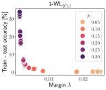
(a) $C_{3}$

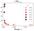
(b) $C_{4}$

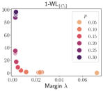
(c) $C_{5}$

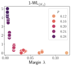
(d) $K_{4}$

Figure 1: Plot illustrating the relation between the margin and generalization error for the ER graphs for different choices of $\mathcal{F}$.

6.1 Results and discussion

In the following we answer questions Q1 to Q4.

Q1 (“Does adding expressive power make datasets more linearly separable?”)

See Tables 1, 5 and 7 (in the appendix). Table 1 confirms Proposition 12, i.e., the $1$-WL and $1$-WLOA kernels do not achieve accuracies better than random and cannot linearly separate the training data. The $1$-WL_F and $1$-WLOA_F kernel linearly separate the data while achieving perfect test accuracies. In addition, Table 5 also confirms this for the ER graphs, i.e., for all datasets, the $1$-WL and $1$-WLOA kernels cannot separate the training data while the $1$-WL_F and $1$-WLOA_F can. Moreover, the subgraph-based kernels achieve the overall best predictive performance over all datasets, e.g., on the dataset using edge probability 0.2 and $\mathcal{F}=\{C_{5}\}$ the test accuracies of the $1$-WL_F improves over the $1$-WL by more than 57 %. Similar effects can be observed for the MPNN architectures; see Table 7.

Q2 (“Can the increased predictive performance of a more expressive variant of the $1$-WL algorithm be explained by an increased margin?”)

See Tables 2, 5 and 1 (in the appendix). On the TUDatasets, an increased margin often leads to less difference between train and test accuracy; see Table 2. For example, on the Proteins datasets, the $1$-WL_F, for all $\mathcal{F}$, leads to a larger difference, while its margin is always strictly smaller than $1$-WL’s margin. Hence, the empirical results align with our theory, i.e., a smaller margin worsens the generalization error. Similar effects can be observed for all other datasets, except Mutag. On the ER dataset, comparing the $1$-WL and $1$-WL_F, for all $\mathcal{F}$, we can clearly confirm the theoretical results. That is, the $1$-WL cannot separate any dataset with a positive margin, while the $1$-WL_F can, and we observe a decreased difference between $1$-WL_F’s train and test accuracies compared to the $1$-WL. Analyzing the $1$-WL_F further, for all $\mathcal{F}$, a decreasing margin always results in an increased difference between test and train accuracies. For example, for $\mathcal{F}=\{C_{4}\}$ and $p=0.05$, the $1$-WL_F achieves a margin of 0.037 with a difference of 0.1 %, for $p=0.1$, it achieves a margin of 0.009 with a difference of 1.8 %, for $p=0.1$, it achieves a margin of 0.002 with a difference of 31.2 %, and, for $p=0.3$, it achieve a margin of 0.003 with difference of 95.8 %, confirming the theoretical results. Moreover, see Figure 1 of visual illustration of this observation.

Q3 (“Does the $1$-WLOA_F lead to increased predictive performance?”)

See Tables 1, 5 and 2 (in the appendix). Table 2 shows that the $1$-WLOA_F kernel performs similarly to the $1$-WL_F, while sometimes achieving better accuracies, e.g., on the PTC_FM and PTC_MR datasets. Table 1 confirms this observation for the empirical verification of Proposition 12, i.e., the $1$-WLOA_F achieve perfect accuracy scores. The results are less clear for the ER datasets. On some datasets, e.g., edge probability 0.05, the $1$-WLOA_F performs similarly to the $1$-WL_F architecture. However, the algorithm leads to significantly worse predictive performance on other datasets. We speculate this is due to numerical problems of the kernelized SVM implementation.

Q4 (“Do the results lift to MPNNs?”)

See Tables 1, 6 and 7 (in the appendix). Table 1 shows that Proposition 12 also lifts to MPNNs, i.e., like the $1$-WL_F kernel, the MPNN_F architecture achieves perfect prediction accuracies while the standard MPNNs does not perform better than random. In addition, on the TUDatasets, the MPNN_F architecture clearly outperforms the standard MPNN over all datasets; see Table 6. For example, on the Enzymes dataset, the MPNN_F architecture beats the MPNN by at least 7 %, for all subgraph choices. This observation holds across all datasets. Moreover, the MPNN_F architectures also achieve better predictive performance on all ER datasets, see Table 7, compared to MPNNs. For example on the dataset using edge probability 0.2 and $\mathcal{F}=\{C_{5}\}$, the test accuracies of the MPNN_F architecture improves over the MPNN by more than 52 %.

Table 3: Mean train, test accuracies, and margins of kernel architectures on ER graphs for different levels of sparsity and different subgraphs. Nls—Not linearly separable. Nb—Only one class in dataset.

Subgraph	Algorithm	Edge probability
		0.05	0.1	0.2	0.3
$C_{3}$	$1$-WL	94.2 $\pm 1.7$ 88.6 $\pm 0.7$ Nls	96.3 $\pm 4.6$ 42.12 $\pm 1.7$ 0.013 $\pm 0.001$	44.1 $\pm 12.4$ 11.2 $\pm$ Nls	38.4 $\pm 5.0$ 6.99 $\pm 1.1$ Nls
	$1$-WLOA	100.0 $\pm 0.0$ 87.9 $\pm 0.1$ Dnc	100.0 $\pm 0.0$ 44.6 $\pm 1.1$ Dnc	100.0 $\pm 0.0$ 11.5 $\pm 0.9$ Dnc	100.0 $\pm 0.0$ 5.2 $\pm 0.3$ Dnc
	$1$-WLF	100.0 $\pm 0.0$ 100.0 $\pm 0.0$ 0.037 $\pm 0.0$	100.0 $\pm 0.0$ 99.7 $\pm 0.1$ 0.009 $<0.001$	100.0 $\pm 0.0$ 100.0 $\pm 0.4$ 0.002 $<0.001$	99.1 $\pm 0.2$ 64.7 $\pm 0.8$ 0.001 $<0.001$
	$1$-WLOAF	100.0 $\pm 0.0$ 98.6 $\pm 0.0$ Dnc	100.0 $\pm 0.0$ 93.8 $\pm 0.3$ Dnc	100.0 $\pm 0.0$ 42.0 $\pm 1.0$ Dnc	100.0 $\pm 0.0$ 7.4 $\pm 0.2$ Dnc
$C_{4}$	$1$-WL	95.1 $\pm 1.0$ 92.3 $\pm 0.2$ Nls	89.7 $\pm 3.9$ 46.8 $\pm 0.8$ Nls	48.7 $\pm 10.1$ 5.4 $\pm 0.5$ Nls	46.6 $\pm 10.8$ 2.2 $\pm 0.4$ Nls
	$1$-WLOA	100.0 $\pm 0.0$ 92.6 $\pm 0.0$ Dnc	100.0 $\pm 0.0$ 49.6 $\pm 0.8$ Dnc	100.0 $\pm 0.0$ 5.13 $\pm 0.6$ Dnc	100.0 $\pm 0.0$ 1.7 $\pm 0.3$ Dnc
	$1$-WLF	100.0 $\pm 0.0$ 99.9 $\pm 0.1$ 0.037 $\pm 0.001$	100.0 $\pm 0.0$ 98.2 $\pm 0.2$ 0.009 $<0.001$	100.0 $0.0$ 78.9 $\pm 0.6$ 0.002 $<0.001$	100.0 $\pm 0.0$ 7.3 $\pm 0.4$ 0.002 $<0.001$
	$1$-WLOAF	100.0 $\pm 0.0$ 99.3 $<0.1$ Dnc	100.0 $\pm 0.0$ 93.7 $\pm 0.2$ Dnc	100.0 $\pm$ 22.4 $\pm 0.9$ Dnc	100.0 $\pm 0.0$ 2.8 $\pm 0.6$ Dnc
$C_{5}$	$1$-WL	97.2 $\pm 0.5$ 95.8 $\pm 0.3$ Nls	69.3 $\pm 6.6$ 53.5 $\pm 0.6$ Nls	65.1 $\pm 14.9$ 4.3 $\pm 0.7$ Nls	64.8 $\pm 9.9$ 1.26 $\pm 0.2$ Nls
	$1$-WLOA	100.0 $\pm 0.0$ 95.9 $\pm 0.0$ Dnc	100.0 $\pm 0.0$ 54.2 $\pm 0.3$ Dnc	100.0 $\pm 0.0$ 4.7 $\pm 0.5$ Dnc	100.0 $\pm 0.0$ 1.4 $\pm 0.5$ Dnc
	$1$-WLF	100.0 $\pm 0.0$ 99.9 $\pm 0.0$ 0.058 $\pm 0.001$	100.0 $\pm 0.0$ 98.4 $\pm 0.2$ 0.012 $<0.001$	100.0 $\pm 0.0$ 68.8 $\pm 0.5$ 0.002 $<0.001$	100.0 $\pm 0.0$ 4.2 $\pm 0.5$ 0.003 $<0.001$
	$1$-WLOAF	100.0 $\pm 0.0$ 99.5 $\pm 0.0$ Dnc	100.0 $\pm 0.0$ 91.8 $\pm 0.4$ Dnc	100.0 $\pm 0.0$ 20.0 $\pm 0.0$ Dnc	100.0 $\pm 0.0$ 2.6 $\pm 0.2$ Dnc
$K_{4}$	$1$-WL	Nb	99.4 $<0.1$ 99.4 $\pm 0.0$ Nls	78.0 $\pm 0.6$ 77.7 $\pm 0.3$ Nls	68.7 $\pm 9.9$ 17.1 $\pm 0.9$ Nls
	$1$-WLOA	Nb	100.0 $\pm 0.0$ 99.4 $\pm 0.0$ Dnc	100.0 $\pm 0.0$ 77.8 $\pm 0.3$ Dnc	100.0 $\pm 0.0$ 20.6 $\pm 0.9$ Dnc
	$1$-WLF	Nb	100.0 $\pm 0.0$ 100.0 $\pm 0.0$ 0.122 $\pm 0.0$	100.0 $\pm 0.0$ 99.9 $\pm 0.1$ 0.022 $<0.001$	100.0 $\pm 0.0$ 94.8 $\pm 0.4$ 0.004 $<0.001$
	$1$-WLOAF	Nb	100.0 $\pm 0.0$ 99.4 $\pm 0.0$ Dnc	100.0 $\pm 0.0$ 97.8 $\pm 0.1$ Dnc	100.0 $\pm 0.0$ 74.6 $\pm 0.6$ Dnc

7 Conclusion

Here, we focused on determining the precise conditions under which increasing the expressive power of MPNN or kernel architectures leads to a provably increased generalization performance. When viewed through graph isomorphism, we first showed that an architecture’s expressivity offers limited insights into its generalization performance. Additionally, we focused on augmenting $1$-WL with subgraph information and derived tight upper and lower bounds for the architectures’ VC dimension parameterized by the margin. Based on this, we derived data distributions where increased expressivity either leads to improved generalization performance or not. Finally, we introduced variations of expressive $1$-WL-based kernels and neural architectures with provable generalization properties. Our empirical study confirmed the validity of our theoretical findings.

Our theoretical results constitute an essential initial step in unraveling the conditions under which more expressive MPNN and kernel architectures yield enhanced generalization performance. Hence, our theory lays a solid foundation for the systematic and principled design of novel expressive MPNN architectures.

Appendix A Simple MPNNs

Here, we provide more details on the simple MPNNs mentioned in Section 2.3. That is, for given $d$ and $L\in\mathbb{N}$, we define the class $\textsf{MPNN}_{\mathsf{mlp}}(d,L)$ of simple MPNNs as $L$-layer MPNNs for which, according to Equation 1, for each $t\in[L]$, the aggregation function $\mathsf{AGG}^{(t)}$ is summation and the update function $\mathsf{UPD}^{(t)}$ is a multilayer perceptron $\mathsf{mlp}^{(t)}\colon\mathbb{R}^{2d}\to\mathbb{R}^{d}$ of width at most $d$. Similarly, the readout function in Equation 2 consists of a multilayer perceptron $\mathsf{mlp}\colon\mathbb{R}^{d}\to\mathbb{R}^{d}$ applied on the sum of all vertex features computed in layer $L$. More specifically, MPNNs in $\textsf{MPNN}_{\mathsf{mlp}}(d,L)$ compute on a labeled graph $G=(V(G),E(G),\ell)$ with $d$-dimensional initial vertex features $\mathbf{h}_{v}^{(0)}\in\mathbb{R}^{d}$, consistent with $\ell$, the following vertex features, for each $v\in V(G)$,

$$\mathbf{h}_{v}^{(t)}\coloneqq\mathsf{mlp}^{(t)}\Bigl{(}\mathbf{h}_{v}^{(t-1)},\sum_{u\in N(v)}\mathbf{h}_{u}^{(t-1)}\Bigr{)}\in\mathbb{R}^{d},$$

for $t\in[L]$, and

$$\mathbf{h}_{G}\coloneqq\mathsf{mlp}\Bigl{(}\sum_{v\in V(G)}\mathbf{h}_{v}^{{(L)}}\Bigr{)}\in\mathbb{R}^{d}.$$

Note that the class $\textsf{MPNN}_{\mathsf{mlp}}(d,L)$ encompasses the GNN architecture derived in Morris et al. [86] that has the same expressive power as the $1$-WL in distinguishing non-isomorphic graphs.

Appendix B Proofs missing from the main paper

Here, we outline proofs missing in the main paper.

B.1 Fundamentals

Here, we prove some fundamental statements for later use.

Margin optimization

Let $(\mathbf{x}_{1},y_{1}),\ldots,(\mathbf{x}_{n},y_{n})\in\mathbb{R}^{d}\times\{0,1\}$, $d>0$, be a linearly separable sample, and let $I^{+}\coloneqq\{i\in[n]\mid y_{i}=1\}$ and $I^{-}\coloneqq\{i\in[n]\mid y_{i}=0\}$. Consider the well-known alternative optimization problem for finding the minimum distance between the convex sets induced by the two classes, i.e.,

$$2\lambda\coloneqq\min_{\boldsymbol{\alpha}\in\mathbb{R}^{|I^{+}|},\boldsymbol{\beta}\in\mathbb{R}^{|I^{-}|}} \lVert\mathbf{x}^{+}_{\boldsymbol{\alpha}}-\mathbf{x}^{-}_{\boldsymbol{\beta}}\rVert$$ (5)

s.t. $$\mathbf{x}^{+}_{\boldsymbol{\alpha}}=\sum_{i\in I^{+}}\alpha_{i}\mathbf{x}_{i},\quad\mathbf{x}^{-}_{\boldsymbol{\beta}}=\sum_{j\in I^{-}}\beta_{j}\mathbf{x}_{j}$$

$$\sum_{i\in I^{+}}\alpha_{i}=1,\quad\sum_{j\in I^{-}}\beta_{j}=1,$$

$$\forall\,i\in I^{+},j\in I^{-}\colon\alpha_{i}\geq 0,\beta_{j}\geq 0,$$

where $\boldsymbol{\alpha}$ and $\boldsymbol{\beta}$ are the variables determining the convex combinations for both the positive and negative classes. Moreover, $\lambda$ is exactly the margin that is computed by the typical hard-margin SVM. We can describe $\lVert\mathbf{x}^{+}_{\boldsymbol{\alpha}}-\mathbf{x}^{-}_{\boldsymbol{\beta}}\rVert^{2}$ by a sum of pairwise distances.

$$\bigg{\lVert}\mathbf{x}^{+}_{\boldsymbol{\alpha}}-\mathbf{x}^{-}_{\boldsymbol{\beta}}\bigg{\rVert}^{2} =\bigg{\lVert}\sum_{i\in I^{+}}\alpha_{i}\mathbf{x}_{i}-\sum_{j\in I^{-}}\beta_{j}\mathbf{x}_{j}\bigg{\rVert}^{2}$$

$$=\bigg{\lVert}\sum_{i\in I^{+}}\alpha_{i}\mathbf{x}_{i}\sum_{j\in I^{-}}\beta_{j}-\sum_{j\in I^{-}}\beta_{j}\mathbf{x}_{j}\sum_{i\in I^{+}}\alpha_{i}\bigg{\rVert}^{2}$$

$$=\bigg{\lVert}\sum_{i\in I^{+}}\sum_{j\in I^{-}}\alpha_{i}\beta_{j}\mathbf{x}_{i}-\sum_{i\in I^{+}}\sum_{j\in I^{-}}\alpha_{i}\beta_{j}\mathbf{x}_{j}\bigg{\rVert}^{2}$$

$$=\bigg{\lVert}\sum_{(i,j)\in I^{+}\times I^{-}}\delta_{i,j}(\mathbf{x}_{i}-\mathbf{x}_{j})\bigg{\rVert}^{2}\quad(\delta_{i,j}\coloneqq\alpha_{i}\beta_{j})$$

$$=\sum_{(i,j)\in I^{+}\times I^{-}}\sum_{(k,l)\in I^{+}\times I^{-}}\delta_{i,j}\delta_{k,l}(\mathbf{x}_{i}-\mathbf{x}_{j})^{\intercal}(\mathbf{x}_{k}-\mathbf{x}_{l})$$

$$=\sum_{(i,j),(k,l)\in I^{+}\times I^{-}}\delta_{i,j}\delta_{k,l}(-\mathbf{x}^{\intercal}_{i}\mathbf{x}_{l}-\mathbf{x}^{\intercal}_{j}\mathbf{x}_{k}+\mathbf{x}^{\intercal}_{i}\mathbf{x}_{k}+\mathbf{x}^{\intercal}_{j}\mathbf{x}_{l})$$

$$=\frac{1}{2}\sum_{\mathclap{(i,j),(k,l)\in I^{+}\times I^{-}}}\delta_{i,j}\delta_{k,l}(\lVert\mathbf{x}_{i}-\mathbf{x}_{l}\rVert^{2}+\lVert\mathbf{x}_{j}-\mathbf{x}_{k}\rVert^{2}-\lVert\mathbf{x}_{i}-\mathbf{x}_{k}\rVert^{2}-\lVert\mathbf{x}_{j}-\mathbf{x}_{l}\rVert^{2}).$$ (6)

We remark that the pairwise distances indexed by $(i,l)$ and $(j,k)$ represent inter-class distances, since $y_{i}=y_{k}=1$ and $y_{j}=y_{l}=0$. Along the same line, the pairwise distances indexed by $(i,k)$ and $(j,l)$ represent intra-class distances.

Proposition 25.

Let $(\mathbf{x}_{1},y_{1}),\dotsc,(\mathbf{x}_{n},y_{n})$ and $(\tilde{\mathbf{x}}_{1},y_{1}),\dots,(\tilde{\mathbf{x}}_{n},y_{n})$ in $\mathbb{R}^{d}$ be two linearly-separable samples, with margins $\lambda$ and $\tilde{\lambda}$, respectively, with the same labels $y_{i}\in\{0,1\}$. If

$$\min_{y_{i}\neq y_{j}}\lVert\tilde{\mathbf{x}}_{i}-\tilde{\mathbf{x}}_{j}\rVert^{2}-\lVert\mathbf{x}_{i}-\mathbf{x}_{j}\rVert^{2}>\max_{y_{i}=y_{j}}\lVert\tilde{\mathbf{x}}_{i}-\tilde{\mathbf{x}}_{j}\rVert^{2}-\lVert\mathbf{x}_{i}-\mathbf{x}_{j}\rVert^{2},$$ (7)

then $\tilde{\lambda}>\lambda$. That is, we get an increase in margin if the minimum increase in distances between classes considering the two samples is strictly larger than the maximum increase in distance within each class.

Proof.

Let

$$\Delta_{\text{min}}\coloneqq\min_{y_{i}\neq y_{j}}\lVert\tilde{\mathbf{x}}_{i}-\tilde{\mathbf{x}}_{j}\rVert^{2}-\lVert\mathbf{x}_{i}-\mathbf{x}_{j}\rVert^{2},$$

and

$$\Delta_{\text{max}}\coloneqq\max_{y_{i}=y_{j}}\lVert\tilde{\mathbf{x}}_{i}-\tilde{\mathbf{x}}_{j}\rVert^{2}-\lVert\mathbf{x}_{i}-\mathbf{x}_{j}\rVert^{2}.$$

By Equation 7, $\Delta_{\text{min}}>\Delta_{\text{max}}$. Starting at Section B.1,

$$\lVert\mathbf{x}^{+}_{\boldsymbol{\alpha}}-\mathbf{x}^{-}_{\boldsymbol{\beta}}\rVert^{2} =\frac{1}{2}\sum_{(i,j)}\sum_{(k,l)}\alpha_{i,j}\alpha_{k,l}(\lVert\mathbf{x}_{i}-\mathbf{x}_{l}\rVert^{2}+\lVert\mathbf{x}_{j}-\mathbf{x}_{k}\rVert^{2}-\lVert\mathbf{x}_{i}-\mathbf{x}_{k}\rVert^{2}-\lVert\mathbf{x}_{j}-\mathbf{x}_{l}\rVert^{2})$$

$$\begin{split}&<\frac{1}{2}\sum_{(i,j)}\sum_{(k,l)}\alpha_{i,j}\alpha_{k,l}(\lVert\mathbf{x}_{i}-\mathbf{x}_{l}\rVert^{2}+\Delta_{\text{min}}+\lVert\mathbf{x}_{j}-\mathbf{x}_{k}\rVert^{2}+\Delta_{\text{min}}\\ &\quad\quad\quad\quad\quad\quad\quad\quad-\lVert\mathbf{x}_{i}-\mathbf{x}_{k}\rVert^{2}-\Delta_{\text{max}}-\lVert\mathbf{x}_{j}-\mathbf{x}_{l}\rVert^{2}-\Delta_{\text{max}}\end{split}$$

$$\leq\frac{1}{2}\sum_{(i,j)}\sum_{(k,l)}\alpha_{i,j}\alpha_{k,l}(\lVert\tilde{\mathbf{x}}_{i}-\tilde{\mathbf{x}}_{l}\rVert^{2}+\lVert\tilde{\mathbf{x}}_{j}-\tilde{\mathbf{x}}_{k}\rVert^{2}-\lVert\tilde{\mathbf{x}}_{i}-\tilde{\mathbf{x}}_{k}\rVert^{2}-\lVert\tilde{\mathbf{x}}_{j}-\tilde{\mathbf{x}}_{l}\rVert^{2})$$

$$=\lVert\tilde{\mathbf{x}}^{+}_{\boldsymbol{\alpha}}-\tilde{\mathbf{x}}^{-}_{\boldsymbol{\alpha}}\rVert^{2},$$

where $\tilde{\mathbf{x}}^{+}_{\boldsymbol{\alpha}}$ and $\tilde{\mathbf{x}}^{-}_{\boldsymbol{\alpha}}$ are derived from applying the optimization (5) to the datapoints $(\tilde{\mathbf{x}}_{1},y_{1}),\allowbreak\dots,\allowbreak(\tilde{\mathbf{x}}_{n},y_{n})$.

In the following, we omit all of the conditions from Equation 5 for simplicity. Let $\mathbf{x}^{+*}$ and $\mathbf{x}^{-*}$ be the representatives of the optimal solution to Equation 5, then

$$\forall\boldsymbol{\alpha}:\gamma=\lVert\mathbf{x}^{+*}-\mathbf{x}^{-*}\rVert\leq\lVert\mathbf{x}^{+}_{\boldsymbol{\alpha}}-\mathbf{x}^{-}_{\boldsymbol{\alpha}}\rVert.$$

Hence,

$$\forall\boldsymbol{\alpha}:\gamma=\lVert\mathbf{x}^{+*}-\mathbf{x}^{-*}\rVert\leq\lVert\mathbf{x}^{+}_{\boldsymbol{\alpha}}-\mathbf{x}^{-}_{\boldsymbol{\alpha}}\rVert<\lVert\tilde{\mathbf{x}}^{+}_{\boldsymbol{\alpha}}-\tilde{\mathbf{x}}^{-}_{\boldsymbol{\alpha}}\rVert,$$

which implies that

$$\gamma<\min_{\boldsymbol{\alpha}}\lVert\tilde{\mathbf{x}}^{+}_{\boldsymbol{\alpha}}-\tilde{\mathbf{x}}^{-}_{\boldsymbol{\alpha}}\rVert\eqqcolon\tilde{\gamma},$$

showing the desired result. ∎

Concatenating feature vectors

We will consider concatenating two feature vectors and analyze how this affects attained margins. To this end, let $X\coloneqq\{(\mathbf{x}_{i},y_{i})\in\mathbb{R}^{d}\times\{0,1\}\mid i\in[n]\}$. When we split up $\mathbb{R}^{d}$ into $\mathbb{R}^{d_{1}}\times\mathbb{R}^{d_{2}}$, we write $\mathbf{x}_{i}\coloneqq(\mathbf{x}_{i}^{1},\mathbf{x}_{i}^{2})$ with $\mathbf{x}_{i}^{1}\in\mathbb{R}^{d_{1}}$ and $\mathbf{x}_{i}^{2}\in\mathbb{R}^{d_{2}}$.

Proposition 26.

If $X\coloneqq\{(\mathbf{x}_{1},y_{1}),\dotsc,(\mathbf{x}_{n},y_{n})\}$ is a sample, such that

1. $(\mathbf{x}^{1}_{1},y_{1}),\dotsc,(\mathbf{x}^{1}_{n},y_{n})$ is $(r_{1},\gamma_{1})$-separable and

2. $(\mathbf{x}^{2}_{1},y_{1}),\dotsc,(\mathbf{x}^{2}_{n},y_{n})$ is $(r_{2},\gamma_{2})$-separable,

then $(\mathbf{x}_{1},y_{1}),\dots,(\mathbf{x}_{n},y_{n})$ is $(\sqrt{r_{1}^{2}+r_{2}^{2}},\sqrt{\gamma_{1}^{2}+\gamma_{2}^{2}})$-separable.

Proof.

Let $I\coloneqq I^{+}\,\dot{\cup}\,I^{-}$ satisfying $y_{i}=1$ if, and only, if $i\in I^{+}$ and $y_{i}=0$ if, and only, if $i\in I^{-}$, $p\coloneqq|I|$, $p^{+}\coloneqq|I^{+}|$ and $p^{-}\coloneqq|I^{-}|$. Further, let $\mathbf{x}_{i}^{+}\coloneqq\mathbf{x}_{i}$, $(\mathbf{x}_{i}^{1})^{+}\coloneqq(\mathbf{x}_{i}^{1},0)$, $(\mathbf{x}_{i}^{2})^{+}\coloneqq(0,\mathbf{x}_{i}^{2})$ for $i\in I^{+}$, and $\mathbf{x}_{i}^{-}\coloneqq\mathbf{x}_{i}$, $(\mathbf{x}_{i}^{1})^{-}\coloneqq(\mathbf{x}_{i}^{1},0)$, and $(\mathbf{x}_{i}^{2})^{-}\coloneqq(0,\mathbf{x}_{i}^{2})$ for $i\in I^{-}$. We collect $\mathbf{x}_{i}^{+}$, $\mathbf{x}_{i}^{-}$, $(\mathbf{x}_{i}^{1})^{+}$, $(\mathbf{x}_{i}^{2})^{+}$, $(\mathbf{x}_{i}^{1})^{-}$, and $(\mathbf{x}_{i}^{2})^{-}$ into matrices $\mathbf{X}^{+}\in\mathbb{R}^{p^{+}\times d}$, $\mathbf{X}^{-}\in\mathbb{R}^{p^{-}\times d}$, $\mathbf{X}_{1}^{+}$, $\mathbf{X}_{2}^{+}\in\mathbb{R}^{p^{+}\times d}$, and $\mathbf{X}_{1}^{-},\mathbf{X}_{2}^{-}\in\mathbb{R}^{p^{-}\times d}$.

The margins $\gamma_{1}$, $\gamma_{2}$, and $\gamma$ (the margin of $(\mathbf{x}_{1},y_{1}),\dots,(\mathbf{x}_{n},y_{n})$) are given by

$$\gamma_{1}\coloneqq\min_{\boldsymbol{\alpha}\in(\mathbb{R}^{+,p^{+}},\boldsymbol{\beta}\in\mathbb{R}^{+,p^{-}},\mathbf{1}^{\intercal}\boldsymbol{\alpha}=1=\mathbf{1}^{\intercal}\boldsymbol{\beta}}\|(\mathbf{X}^{+}_{1})^{\intercal}\boldsymbol{\alpha}-(\mathbf{X}^{-}_{1})^{\intercal}\boldsymbol{\beta}\|$$

$$\gamma_{2}\coloneqq\min_{\boldsymbol{\alpha}\in\mathbb{R}^{+,p^{+}},\boldsymbol{\beta}\in\mathbb{R}^{+,p^{-}},\mathbf{1}^{\intercal}\boldsymbol{\alpha}=1=\mathbf{1}^{\intercal}\boldsymbol{\beta}}\|(\mathbf{X}^{+}_{2})^{\intercal}\boldsymbol{\alpha}-(\mathbf{X}^{-}_{2})^{\intercal}\boldsymbol{\beta}\|$$

$$\gamma\coloneqq\min_{\boldsymbol{\alpha}\in\mathbb{R}^{+,p^{+}},\boldsymbol{\beta}\in\mathbb{R}^{+,p^{-}},\mathbf{1}^{\intercal}\boldsymbol{\alpha}=1=\mathbf{1}^{\intercal}\boldsymbol{\beta}}\|(\mathbf{X}^{+})^{\intercal}\boldsymbol{\alpha}-(\mathbf{X}^{-})^{\intercal}\boldsymbol{\beta}\|,$$

where $\mathbb{R}^{+}$ is the set of positive real numbers and $\mathbf{1}$ is a vector of ones of appropriate size. We have

$$\|(\mathbf{X}^{+})^{\intercal}\boldsymbol{\alpha}-(\mathbf{X}^{-})^{\intercal}\boldsymbol{\beta}\|^{2} =\|(\mathbf{X}_{1}^{+})^{\intercal}{\alpha}_{1}+(\mathbf{X}_{2}^{+})^{\intercal}{\alpha}_{2}-(\mathbf{X}_{1}^{-})^{\intercal}{\beta}_{1}-(\mathbf{X}_{2}^{-})^{\intercal}{\beta}_{2}\|^{2}$$

$$=\|((\mathbf{X}_{1}^{+})^{\intercal}{\alpha}_{1}-(\mathbf{X}_{1}^{-})^{\intercal}{\beta}_{1})+((\mathbf{X}_{2}^{+})^{\intercal}{\alpha}_{2}-(\mathbf{X}_{2}^{-})^{\intercal}{\beta}_{2})\|^{2}$$

$$=\|(\mathbf{X}_{1}^{+})^{\intercal}{\alpha}_{1}-(\mathbf{X}_{1}^{-})^{\intercal}{\beta}_{1}\|^{2}+\|(\mathbf{X}_{2}^{+})^{\intercal}{\alpha}_{2}-(\mathbf{X}_{2}^{-})^{\intercal}{\beta}_{2}\|^{2}.$$

The latter terms attain, by assumption, minimal values of $\gamma_{1}$ and $\gamma_{2}$, respectively. Thus, $\gamma^{2}=\gamma_{1}^{2}+\gamma_{2}^{2}$. Also note that $\|\mathbf{x}_{i}\|^{2}\leq r_{1}^{2}+r_{2}^{2}$ for all $i\in I$. This implies that $(\mathbf{x}_{1},y_{1}),\dotsc,(\mathbf{x}_{n},y_{n})$ is $(\sqrt{r_{1}^{2}+r_{2}^{2}},\sqrt{\gamma_{1}^{2}+\gamma_{2}^{2}})$-separable. ∎

Existence of regular graphs

The following result ensures the existence of enough regular graphs needed for the proof of Theorem 4 and its variants.

Lemma 27.

For any even $n$ and all $i\in\{0,\dots,n-1\}$, there exists an $i$-regular graph with one orbit containing all vertices.

Proof.

Let $n$ be even, and let $c$ be an arbitrary natural number. We define

$$E_{\text{odd}}\coloneqq\{(i,i+\nicefrac{{n}}{{2}})\mid i\in[\nicefrac{{n}}{{2}}]\},$$

and

$$E_{c}\coloneqq\{(i,i+c\text{ mod }n)\mid i\in[n]\},$$

where mod is the modulo operator with equivalence classes $[n]$. It is easily verified that for any $C\in\mathbb{N}$, $([n],\bigcup_{c\in[C]}E_{c})$ is a $2C$-regular graph. Also, $([n],E_{\text{odd}}\cup\bigcup_{c\in[C]}E_{c})$ is a $2C+1$-regular graph. The permutation, in cycle notation, $(1,2,\dots,n)$ is an automorphism for both graphs, implying that all vertices are in the same orbit. ∎

Remark 28.

For any odd $n$, no $i$-regular graph exists with $i$ odd. This is a classical textbook question that can be verified by handshaking. For regular graphs,

$$\sum_{i\in[n]}\textsf{deg}(i)=i\cdot n.$$

Summing the degrees for each vertex counts each edge twice. Thus, $i\cdot n$ must be even, and since $n$ is odd, $i$ must be even.

B.2 Expressive power of enhanced variants

We now prove results on the expressive power of the $1$-WL_F.

Proposition 29 (Proposition 1 in the main paper).

Let $G$ be a graph and $\mathcal{F}$ be a set of graphs. Then, for all rounds, the $1$-WL_F distinguishes at least the same vertices as the $1$-WL.

Proof.

Using, induction on $t$, we show that, for all vertices $v,w\in V(G)$,

$$C^{1,\mathcal{F}}_{t}(v)=C^{1,\mathcal{F}}_{t}(w)\text{ implies }C^{1}_{t}(v)=C^{1}_{t}(w).$$ (8)

The base case, $t=0$, is clear since $1$-WL_F refines the single color class induced by $C^{1}_{0}$. For the induction, assume that Equation 8 holds and assume that, $C^{1,\mathcal{F}}_{t+1}(v)=C^{1,\mathcal{F}}_{t+1}(w)$ holds. Hence, $C^{1}_{t}(v)=C^{1}_{t}(w)$ and

$$\{\!\!\{C^{1,\mathcal{F}}_{t}(a)\mid a\in N(v)\}\!\!\}=\{\!\!\{C^{1,\mathcal{F}}_{t}(b)\mid b\in N(w)\}\!\!\}$$

holds. Hence, there is a color-preserving bijection $\varphi\colon N(v)\to N(w)$ between the above two multisets, i.e., $C^{1,\mathcal{F}}_{t}(a)=C^{1,\mathcal{F}}_{t}(\varphi(a))$, for $a\in N(v)$. Hence, by Equation 8, $C^{1}_{t}(a)=C^{1}_{t}(\varphi(a))$, for $a\in N(v)$. Consequently, it holds that $C^{1}_{t+1}(v)=C^{1}_{t+1}(w)$, proving the desired result. ∎

In addition, by choosing the set of graphs $\mathcal{F}$ appropriately, $1$-WL_F gets strictly more expressive than $1$-WL in distinguishing non-isomorphic graphs.

Proposition 30 (Proposition 2 in the main paper.).

For every $n\geq 6$, there exists at least one pair of non-isomorphic graphs and a set of graphs $\mathcal{F}$ containing a single constant-order graph, such that, for all rounds, $1$-WL does not distinguish them while $1$-WL_F distinguishes them after a single round.

Proof.

For $n=6$, we can choose a pair of a $6$-cycle and the disjoint union of two $3$-cycles. Since both graphs are $2$-regular, the $1$-WL cannot distinguish them. By choosing $\mathcal{F}=\{C_{3}\}$, the $1$-WL_F distinguishes them. For $n>6$, we can simply pad the graphs with $n-6$ isolated vertices. ∎

B.3 Margin-based upper and lower bounds on the VC dimension of Weisfeiler–Leman-based kernels

We now prove the VC dimension theory results from the main paper. In the following, we will reuse our notation of splitting up $\mathbb{R}^{d}$ into $\mathbb{R}^{d_{1}}\times\mathbb{R}^{d_{2}}$. We write $\mathbf{x}_{i}=(\mathbf{x}_{i}^{(1)},\mathbf{x}_{i}^{(2)})$ with $\mathbf{x}_{i}^{(1)}\in\mathbb{R}^{d_{1}}$ and $\mathbf{x}_{i}^{(2)}\in\mathbb{R}^{d_{2}}$. Further, let $(\mathbf{x}_{i}^{(1)})^{+}\coloneqq(\mathbf{x}_{i}^{(1)},0)$, and $(\mathbf{x}_{i}^{(2)})^{+}\coloneqq(0,\mathbf{x}_{i}^{(2)})$.

Lemma 31 (Lemma 3 in the main paper).

Let $\mathbb{S}\subseteq\mathbb{R}^{d}$. If $\mathbb{S}$ contains $m\coloneqq\lfloor\nicefrac{{r^{2}}}{{\lambda^{2}}}\rfloor$ vectors $\mathbf{b}_{1},\dotsc,\mathbf{b}_{m}\in\mathbb{R}^{d}$ with $\mathbf{b}_{i}:=(\mathbf{b}_{i}^{(1)},\mathbf{b}_{i}^{(2)})$ and $\mathbf{b}_{1}^{(2)},\dotsc,\mathbf{b}_{m}^{(2)}$ being pairwise orthogonal, $\|\mathbf{b}_{i}\|=r^{\prime}$, and $\|\mathbf{b}_{i}^{(2)}\|=r$, then

$$\mathsf{VC}\text{-}\mathsf{dim}(\mathbb{H}_{r^{\prime},\lambda}(\mathbb{S}))\in\Theta(\nicefrac{{r^{2}}}{{\lambda^{2}}}).$$

Proof.

It suffices to show the lower bound. Following the argument in Alon et al. [3], we show that the vectors $\mathbf{b}_{1},\dotsc,\mathbf{b}_{m}$ can be shattered. Indeed, let $A$ and $B$ be two arbitary sets partitioning $[m]$. Consider the vector

$$\mathbf{w}\coloneqq\frac{\lambda}{r^{2}}\Bigg{(}\sum_{i\in A}(\mathbf{b}_{i}^{(2)})^{+}-\sum_{i\in B}(\mathbf{b}_{i}^{(2)})^{+}\Bigg{)}.$$

We observe that, because of assumptions underlying the vectors $\mathbf{b}_{i}$, we have

$$\mathbf{w}^{\intercal}\mathbf{b}_{j}=\begin{cases}\mathopen{}\mathclose{{}\left(\frac{\lambda}{r^{2}}}\right)\cdot(\mathbf{b}_{j}^{(2)})^{\intercal}\mathbf{b}_{j}^{(2)}=\lambda&\text{if $j\in A$}\\ -\mathopen{}\mathclose{{}\left(\frac{\lambda}{r^{2}}}\right)\cdot(\mathbf{b}_{j}^{(2)})^{\intercal}\mathbf{b}_{j}^{(2)}=-\lambda&\text{if $j\in B$}.\end{cases}$$

In other words, $\mathbf{w}$ witnesses that the distance between the convex hull of $\{\mathbf{b}_{i}\mid i\in A\}$ and $\{\mathbf{b}_{i}\mid i\in B\}$ is at least $2\lambda$, implying the result. ∎

Theorem 32 (Theorem 4 in the main paper).

For any $T,\lambda>0$, we have,

$$\mathsf{VC}\text{-}\mathsf{dim}(\mathbb{H}_{\sqrt{T+1}n,\lambda}(\mathcal{E}_{\mathsf{WL}}(n,d_{T})))\in{\Theta}(\nicefrac{{r^{2}}}{{\lambda^{2}}})\text{ for }r=\sqrt{T}n\text{ and }n\geq\nicefrac{{r^{2}}}{{\lambda^{2}}},$$

$$\mathsf{VC}\text{-}\mathsf{dim}(\mathbb{H}_{1,\lambda}(\widebar{\mathcal{E}}_{\mathsf{WL}}(n,d_{T})))\in{\Theta}(\nicefrac{{1}}{{\lambda^{2}}})\text{ for }r=\sqrt{T/(T+1)}\text{ and }n\geq\nicefrac{{r^{2}}}{{\lambda^{2}}}.$$

Proof.

The upper bounds follow from the general upper bound described earlier. For the lower bound, we show that for even $n\geq r^{2}/\lambda^{2}$, there exist $m=\lfloor r^{2}/\lambda^{2}\rfloor$ graphs $G_{1},\dotsc,G_{m}$ in $\mathcal{G}_{n}$ such that the vectors $\mathbf{b}_{i}\coloneqq\phi^{(1)}_{\textsf{WL}}(G_{i})$ and $\widebar{\mathbf{b}}_{i}\coloneqq\widebar{\phi}^{(1)}_{\textsf{WL}}(G_{i})$ satisfy the assumptions of Lemma 31. Indeed, we can simply consider $G_{i}$ to be an $(i-1)$-regular graph of order $n$; see Lemma 27. We break up the feature vectors into two parts: a one-dimensional part corresponding to the information related to the initial color and the remaining part containing all other information. We remark that for the $1$-WL and for unlabeled graphs, all vertices have the same initial color. The interesting information is hence contained in the second part. If we inspect the $1$-WL feature vectors, excluding the initial colors, for $T=1$ of $G_{i}$, we obtain $(0,\dotsc,\underbrace{n}_{\text{pos }i},\dotsc,0)$ in the unnormalized case, and $\frac{1}{\sqrt{1+1}n}(0,\dotsc,\underbrace{n}_{\text{pos }i},\dotsc,0)$ in the normalized case. It is readily verified that $\mathbf{b}_{i}^{(2)}\coloneqq(0,\dotsc,\underbrace{n}_{\text{pos }i},\dotsc,0)$ and $\mathbf{b}_{i}^{(1)}$ being the remaining initial colors are vectors satisfying the assumptions of Lemma 31 in the unnormalized case. For larger $T$, $\mathbf{b}_{i}^{(2)}$ is $\phi^{(1)}_{\textsf{WL}}(G_{i})$ except for the initial colors. Note that $\|\mathbf{b}_{i}^{(2)}\|=\sqrt{T}n=r$ and $\|\mathbf{b}_{i}\|=\sqrt{T+1}n\colon=r^{\prime}$. For the normalized case, one simply needs to rescale with $\nicefrac{{1}}{{r^{\prime}}}$. Note that for $T>0$, $\nicefrac{{1}}{{2}}\leq\nicefrac{{r^{2}}}{{r^{\prime 2}}}<1$. This implies a lower bound of $\Omega(\frac{r^{2}}{\lambda^{2}})$ in the unnormalized case, and $\Omega(\frac{r^{2}}{\lambda^{2}r^{\prime 2}})=\Omega(\frac{1}{\lambda^{2}})$ in the normalized case.

So far, we assumed $n$ to be even. For odd $n$, there is a slight technicality in that we can construct all $r$-regular graphs where $r$ is even, i.e., we can construct $\nicefrac{{n+1}}{{2}}$ regular graphs. Analogously this means for odd $n$ and $\nicefrac{{n+1}}{{2}}\geq r^{2}/\lambda^{2}$, which is equivalent to $n\geq\nicefrac{{2r^{2}}}{{\lambda^{2}}}-1$, by a slight variant of Lemma 31 this implies a lower bound of $\Omega(\nicefrac{{2r^{2}}}{{\lambda^{2}}}-1)=\Omega(\nicefrac{{r^{2}}}{{\lambda^{2}}})$. Analogous to the normalized case can be considered for odd $n$ and results in the same bound, which proves the desired result. ∎

Theorem 33 (Theorem 5 in the main paper).

Let $\mathcal{F}$ be a finite set of graphs. For any $T,\lambda>0$, we have,

$$\mathsf{VC}\text{-}\mathsf{dim}(\mathbb{H}_{\sqrt{T+1}n,\lambda}(\mathcal{E}_{\mathsf{WL},\mathcal{F}}(n,d_{T})))\in{\Theta}(\nicefrac{{r^{2}}}{{\lambda^{2}}})\text{ for }r=\sqrt{T}n\text{ and }n\geq\nicefrac{{r^{2}}}{{\lambda^{2}}}$$

$$\mathsf{VC}\text{-}\mathsf{dim}(\mathbb{H}_{1,\lambda}(\widebar{\mathcal{E}}_{\mathsf{WL},\mathcal{F}}(n,d_{T})))\in{\Theta}(\nicefrac{{1}}{{\lambda^{2}}})\text{ for }r=\sqrt{T/(T+1)}\text{ and }n\geq\nicefrac{{r^{2}}}{{\lambda^{2}}}.$$

Proof.

This proof is analogous to the proof of Theorem 32. Note that in the proof above, we can choose the regular graphs such that all vertices in one graph are in the same orbit; see Lemma 27. This implies that if one vertex is colored according to $\mathcal{F}$, all vertices are colored in the same color, and the feature vectors $\phi^{(1)}_{\textsf{WL},\mathcal{F}}(G_{i})$ look exactly as described before, implying the result. ∎

A careful reader might wonder why we did not consider the initial colors in the proofs above. In the $1$-WL-case, the initial colors are the same for all graphs in $\mathcal{G}_{n}$, i.e., the $1$-WL feature vectors take the form $(n,\dots)$. We could leverage this to reduce the radius of the hypothesis class slightly. However, when considering the $1$-WL_F-case, the graphs in $\mathcal{F}$ change the initial colors. Because of our regular graph construction from Lemma 27, all nodes within one graph share the same color, determined by a subset $F\subseteq\mathcal{F}$, where $F$ contains all graphs that are subgraphs of the regular graph in question. Hence, $2^{|\mathcal{F}|}$ possible initial colorings of graphs in $\mathcal{G}_{n}$ exists. Also, in both cases, our regular graphs are not necessarily orthogonal in the dimensions of these initial colors. Therefore, we disregarded them in the constructions of $\mathbf{w}$ above.

Proposition 34 (Proposition 6 in the main paper).

For any $T,\lambda>0$, we have,

$$\mathsf{VC}\text{-}\mathsf{dim}(\mathbb{H}_{\sqrt{(T+1)n},\lambda}(\mathcal{E}_{\mathsf{WLOA}}(n,d_{T})))\in{\Theta}(\nicefrac{{r^{2}}}{{\lambda^{2}}})\text{ for }r=\sqrt{Tn}\text{ and }n\geq\nicefrac{{r^{2}}}{{\lambda^{2}}},$$

$$\mathsf{VC}\text{-}\mathsf{dim}(\mathbb{H}_{1,\lambda}(\widebar{\mathcal{E}}_{\mathsf{WLOA}}(n,d_{T})))\in{\Theta}(\nicefrac{{1}}{{\lambda^{2}}})\text{ for }r=\sqrt{T/(T+1)}\text{ and }n\geq\nicefrac{{r^{2}}}{{\lambda^{2}}}.$$

Proof.

This proof is analogous to the proof of Theorem 32 except $\|\phi^{(1)}_{\textsf{WLOA}}(G_{i})\|=\sqrt{(T+1)n}\eqqcolon r^{\prime}$ and $\|e_{i}\|=\sqrt{Tn}=r$. This implies a lower bound of $\Omega(\frac{r^{2}}{\lambda^{2}})$ in the unnormalized case, and $\Omega(\frac{r^{2}}{\lambda^{2}r^{\prime 2}})=\Omega(\frac{1}{\lambda^{2}})$ in the normalized case, as desired. ∎

Proposition 35 (Proposition 7 in the main paper).

Let $\mathcal{F}$ be a finite set of graphs. For any $T,\lambda>0$, we have,

$$\mathsf{VC}\text{-}\mathsf{dim}(\mathbb{H}_{\sqrt{(T+1)n},\lambda}(\mathcal{E}_{\mathsf{WLOA},\mathcal{F}}(n,d_{T})))\in{\Theta}(\nicefrac{{r^{2}}}{{\lambda^{2}}})\text{ for }r=\sqrt{Tn}\text{ and }n\geq\nicefrac{{r^{2}}}{{\lambda^{2}}},$$

$$\mathsf{VC}\text{-}\mathsf{dim}(\mathbb{H}_{1,\lambda}(\widebar{\mathcal{E}}_{\mathsf{WLOA},\mathcal{F}}(n,d_{T})))\in{\Theta}(\nicefrac{{1}}{{\lambda^{2}}})\text{ for }r=\sqrt{T/(T+1)}\text{ and }n\geq\nicefrac{{r^{2}}}{{\lambda^{2}}}.$$

Proof.

This proof is analogous to the proofs of Theorems 33 and 34. ∎

B.3.1 Colored margin bounds

Given $T\geq 0$ and $C\subseteq\mathbb{N}$, we say that a graph $G$ has color complexity $(C,T)$ if the first $T$ iterations of $1$-WL assign colors to $G$ in the set $C$. Let $\mathcal{G}_{C,T}$ be the class of all graphs of color complexity $(C,T)$. We note that $\mathcal{G}_{C,T}$ possibly contains infinitely many graphs. Indeed, if $C$ corresponds to the color assigned by $1$-WL to degree two nodes, then $\mathcal{G}_{C,T}$ contains all $2$-regular graphs.

Let $\mathcal{E}(C,T,d)$ be a class of graph embedding methods consisting of mappings from $\mathcal{G}_{C,T}$ to $\mathbb{R}^{d}$. Separability is lifted to the setting by considering the set of partial concepts defined on $\mathcal{G}_{C,T}$, as follows

$$\mathbb{H}_{r,\lambda}(\mathcal{E}(C,T,d))\coloneqq\Big{\{}h\in\{0,1,\star\}^{\mathcal{G}_{C,T}}\mathrel{\Big{|}}\,\forall\, G_{1},\dotsc,G_{s}\in\mathsf{supp}(h)\colon$$

$$( G_{1},h(G_{1})),\dotsc,(G_{s},h(G_{s}))\text{ is $(r,\lambda)$-$\mathcal{E}(n,d)$-separable}\Big{\}}.$$

Let $\widebar{\mathcal{E}}_{\mathsf{WL}}(C,T,d)$ be the class of embeddings corresponding to the normalized $1$-WL kernel, i.e., $\widebar{\mathcal{E}}_{\mathsf{WL}}(C,T,d)\coloneqq\{G\mapsto\widebar{\phi^{(T)}_{\textsf{WL}}}(G)\mid G\in\mathcal{G}_{C,T}\}$. We note that $d$ is a constant depending on $|C|$ and $T$, we denote this constant by $d_{C,T}$. An immediate consequence of the proof of Theorem 4 is that we can obtain a margin-bound for infinite classes of graphs.

Corollary 36.

For any $T>0$, $C\subseteq\mathbb{N}$, and $\lambda>0$, such that $\mathcal{G}_{C,T}$ contains all regular graphs of degree $0,1,\ldots,\nicefrac{{r^{2}}}{{\lambda^{2}}}$, for $r=\sqrt{T/(T+1)}$, we have

$$\mathsf{VC}\text{-}\mathsf{dim}(\mathbb{H}_{1,\lambda}(\widebar{\mathcal{E}}_{\mathsf{WL}}(C,T,d_{C,T})))\in{\Theta}(\nicefrac{{1}}{{\lambda^{2}}})\text{ for }r=\sqrt{T/(T+1).}$$ ∎

B.4 Margin-based bounds on the VC dimension of MPNNs and more expressive architectures

We now lift the above results for the $1$-WL kernel to MPNNs. To prove Theorem 8, we show that $\mathcal{E}_{\textsf{MPNN}}(n,d,T)$ contains $\mathcal{E}_{\mathsf{WL}}(n,d_{T})$. Thereto, the following result shows that MPNNs can compute the $1$-WL feature vector.

Proposition 37.

Let $\mathcal{G}_{n}$ be the set of $n$-order graphs and let $S\subseteq\mathcal{G}_{n}$. Then, for all $T\geq 0$, there exists a sufficiently wide $T$-layered simple MPNN architecture $\mathsf{mpnn}_{n}\colon S\to\mathbb{R}^{d}$, for an appropriately chosen $d>0$, such that, for all $G\in S$,

$$\mathsf{mpnn}_{n}(G)=\phi^{(T)}_{\textsf{WL}}(G).$$

Proof.

The proof follows the construction outlined in the proof of [91, Proposition 2]. Let $s\coloneqq|S|$. Hence, $sn$ is an upper bound for the number of colors computed by $1$-WL over all $s$ graphs in one iteration.

Now, by Morris et al. [86, Theorem 2], there exists an MPNN architecture with feature dimension (at most) $n$ and consisting of $t$ layers such that for each graph $G\in S$ it computes $1$-WL-equivalent vertex features $\mathbf{f}_{v}^{(t)}$ in $\mathbb{R}^{1\times n}$ for $v\in V(G)$. That is, for vertices $v$ and $w$ in $V(G)$ it holds that

$$\mathbf{f}_{v}^{(t)}=\mathbf{f}_{w}^{(t)}\iff C^{1}_{T}(v)=C^{1}_{T}(w).$$

We note, by the construction outlined in the proof of Morris et al. [86, Theorem 2], that $\mathbf{f}_{v}^{(t)}$, for $v\in V(G)$, is defined over the rational numbers. We further note that we can construct a single MPNN architecture for all $s$ graphs by applying Morris et al. [86, Theorem 2] over the disjoint union of the graphs in $S$. This increases the width from $n$ to $sn$. We now show how to compute the $1$-WL feature vector of a single iteration $t$. The overall feature vector can be obtained by (column-wise) concatenation over all layers.

Since the vertex features are rational, there exists a number $M$ in $\mathbb{N}$ such that $M\cdot\mathbf{f}_{v}^{(t)}$ is in $\mathbb{N}^{1\times sn}$ for all $v\in V(G)$ and $G\in S$, i.e., a vector over $\mathbb{N}$. Now, let

$$\mathbf{W}^{\prime}=\begin{bmatrix}K^{sn-1}&\cdots&K^{sn-1}\\ \vdots&\cdots&\vdots\\ K^{0}&\cdots&K^{0}\end{bmatrix}\in\mathbb{N}^{sn\times 2sn},$$

for a sufficiently large $K>0$, then $\mathbf{k}_{v}\coloneqq M\cdot\mathbf{f}_{v}^{(t)}\mathbf{W}^{\prime}$, for vertex $v\in V(G)$ and graph $G\in S$, computes a vector $\mathbf{k}_{v}$ in $\mathbb{N}^{2sn}$ containing $2sn$ occurrences of a natural number uniquely encoding the color of the vertex $v$. We next turn $\mathbf{k}_{v}$ into a one-hot encoding. More specifically, we define

$$\mathbf{h}_{v}^{\prime}=\mathsf{lsig}(\mathbf{k}_{v}\circ(\mathbf{w}^{\prime\prime})^{\intercal}+\mathbf{b}),$$

where $\circ$ denotes element-wise multiplication, with $\mathbf{w}^{\prime\prime}=(1,-1,1,-1,\dotsc,1,-1)\in\mathbb{R}^{2sn}$ and $\mathbf{b}=(-c_{1}-1,c_{1}+1,-c_{2}-1,c_{2}+1,\dotsc,-c_{sn}-1,c_{sn}+1)\in\mathbb{R}^{2sn}$with $c_{i}$ the number encoding the $i$th color under $1$-WL at iteration $t$ on the set $S$. We note that for odd $i$,

$$(h_{v}^{\prime})_{i}\coloneqq\mathsf{lsig}(C^{1}_{t}(v)-c_{i}-1)=\begin{cases}1&C^{1}_{t}(v)\geq c_{i}\\ 0&\text{otherwise}.\end{cases}$$

and for even $i$,

$$(h_{v}^{\prime})_{i}\coloneqq\mathsf{lsig}(-C^{1}_{t}(v)+c_{i}+1)=\begin{cases}1&C^{1}_{t}(v)\leq c_{i}\\ 0&\text{otherwise}.\end{cases}$$

In other words, $((h_{v}^{\prime})_{i},(h_{v}^{\prime})_{i+1})$ are both $1$ if and only if $C^{1}_{t}(v)=c_{i}$. We thus obtain one-hot encoding of the color $C^{1}_{t}(v)$ by combining $((h_{v}^{\prime})_{i},(h_{v}^{\prime})_{i+1})$ using an “AND” encoding (e.g., $\mathsf{lsig}(x+y-1)$) applied to pairs of consecutive entries in $\mathbf{h}_{v}^{\prime}$. That is,

$$\mathbf{h}_{v}\coloneqq\mathsf{lsig}\mathopen{}\mathclose{{}\left(\mathbf{h}_{v}^{\prime}\cdot\begin{pmatrix}1&0&\cdots&0\\ 1&0&\cdots&0\\ 0&1&\cdots&0\\ 0&1&\cdots&0\\ \vdots&\vdots&\ddots&\vdots\\ 0&0&\cdots&1\\ 0&0&\cdots&1\end{pmatrix}-(1,1,\dotsc,1)}\right)\in\mathbb{R}^{sn}.$$

We obtain the overall $1$-WL vector by row-wise summation and concatenation over all layers. We remark that, for a single iteration, the maximal width of the whole construction is $2sn$. ∎

By the above proposition, MPNNs of sufficient width can compute the $1$-WL feature vectors. Moreover, note that the normalization can be included in the MPNN computation. Hence, we can prove the lower bound by simulating the proof of Theorem 4. The upper bound follows by the same arguments as described at the beginning of Section 3.1. The above result can be easily extended to the $1$-WL_F, implying Proposition 9.

Corollary 38.

Let $\mathcal{G}_{n}$ be the set of $n$-order graphs, let $S\subseteq\mathcal{G}_{n}$, and let $\mathcal{F}$ be a set of graphs. Then, for all $T\geq 0$, there exists a sufficiently wide $T$-layered MPNN architecture $\mathsf{mpnn}_{n}\colon S\to\mathbb{R}^{d}$, for an appropriately chosen $d>0$, such that, for all $G\in S$,

$$\mathsf{mpnn}_{n}(G)=\phi^{(T)}_{\text{$1${-}{WL}${}_{\mathcal{F}}$}}(G).$$

Proof sketch.

By definition of the $1$-WL_F, the algorithm is essentially the $1$-WL operating on a specifically vertex-labeled graph. Since Morris et al. [86, Theorem 2] also works for vertex-labeled graphs, the proof technique for Proposition 37 can be straightforwardly lifted to the $1$-WL_F. ∎

We can also extend Proposition 37 to the $1$-WLOA and $1$-WLOA_F, i.e., derive an MPNN architecture that can compute $1$-WLOA’s and $1$-WLOA_F’s feature vectors. By that, we can extend Propositions 6 and 7 to their corresponding MPNN versions.

Proposition 39.

Let $\mathcal{G}_{n}$ be the set of $n$-order graphs and let $S\subseteq\mathcal{G}_{n}$. Then, for all $T\geq 0$, there exists a sufficiently wide $T$-layered MPNN architecture $\mathsf{mpnn}_{n}\colon S\to\mathbb{R}^{d}$, for an appropriately chosen $d>0$, such that, for all $G\in S$,

$$\mathsf{mpnn}_{n}(G)=\phi^{(T)}_{\textsf{WLOA}}(G).$$

Proof.

By Proposition 37, there exists a $T$-layered MPNN architecture $\mathsf{mpnn}_{n}\colon S\to\mathbb{R}^{d}$, for an appropriately chosen $d>0$, such that, for all $G\in S$,

$$\mathsf{mpnn}_{n}(G)=\phi^{(T)}_{\text{$1${-}{WL}}}(G).$$

We now show how to transform $\phi^{(T)}_{\text{$1${-}{WL}}}(G)$ into $\phi^{(T)}_{\textsf{WLOA}}(G)$. We show the transformation for a single iteration $t\leq T$, i.e., transforming $\phi_{t,\text{$1${-}{WL}}}(G)$ into $\phi_{t,\text{$1${-}{WLOA}}}(G)$. Let $C$ denote the number of colors at iteration $t$ of the $1$-WL over all $|S|$ graphs. Since $n$ is finite, $C$ is finite as well. That is, $\phi_{t,\text{$1${-}{WL}}}(G)$ has $C$ entries. Hence, the number of components for $\phi_{t,\textsf{WLOA}}(G)$ is at most $Cn$. By multiplying $\phi_{t,\text{$1${-}{WL}}}(G)$ with an appropriately chosen matrix $\mathbf{M}\in\{0,1\}^{C\times Cn}$, we get a vector $\mathbf{r}\in\mathbb{R}^{Cn}$, where each entry of $\phi_{t,\text{$1${-}{WL}}}(G)$ is repeated $n$ times. Specifically,

$$\mathbf{M}\coloneqq\begin{pmatrix}1&0&\cdots&0\\ 1&0&\cdots&0\\ \vdots&\vdots&\cdots&0\\ 1&0&\cdots&0\\ 0&1&\cdots&0\\ 0&1&\cdots&0\\ \vdots&\vdots&\ddots&0\\ 0&0&\cdots&1\\ 0&0&\cdots&1\\ 0&0&\cdots&\vdots\\ 0&0&\cdots&1\end{pmatrix}\in\{0,1\}^{C\times Cn}.$$

Now let

$$\mathbf{b}\coloneqq(1,2,\dotsc,n,1,2,\dotsc,n,\dotsc,1,2,\dotsc,n)\in\mathbb{R}^{Cn}\quad\text{ and }\quad\mathbf{r^{\prime}}\coloneqq\mathsf{sign}{(\mathbf{r}-\mathbf{b})}.$$

Observe that $\mathbf{r^{\prime}}=\phi_{t,\text{$1${-}{WLOA}}}(G)$, implying the result ∎

In a similar way as for Corollary 38, we can lift the above result to the $1$-WLOA_F.

Corollary 40.

Let $\mathcal{G}_{n}$ be the set of $n$-order graphs, let $S\subseteq\mathcal{G}_{n}$, and let $\mathcal{F}$ be a set of graphs. Then, for all $T\geq 0$, there exists a sufficiently wide $T$-layered MPNN architecture $\mathsf{mpnn}_{n}\colon S\to\mathbb{R}^{d}$, for an appropriately chosen $d>0$, such that, for all $G\in S$,

$$\mathsf{mpnn}_{n}(G)=\phi^{(T)}_{\text{$1${-}{WLOA}${}_{\mathcal{F}}$}}(G).$$ ∎

B.5 Increased separation power of the $1$-WL_F

We now prove how more expressive architectures help to separate the data.

Lemma 41 (Proposition 10 in the main paper).

For every $n\geq 6$, there exists a pair of non-isomorphic $n$-order graphs $(G_{n}$, $H_{n})$ and a graph $F$ such that, for $\mathcal{F}\coloneqq\{F\}$ and for all number of rounds $T\geq 0$, it holds that

$$\bigg{\lVert}\widebar{\phi^{(T)}_{\textsf{WL}}}(G_{n})-\widebar{\phi^{(T)}_{\textsf{WL}}}(H_{n})\bigg{\rVert}=0,\quad\text{ and }\quad\bigg{\lVert}\widebar{\phi^{(T)}_{\textsf{WL},\mathcal{F}}}(G_{n})-\widebar{\phi^{(T)}_{\textsf{WL},\mathcal{F}}}(H_{n})\bigg{\rVert}=\sqrt{2}.$$

Proof.

Let $G_{n}\coloneqq C_{n}$, a cycle on $n$ vertices. Further, let $H_{n}\coloneqq C_{\lceil n/2\rceil}\dot{\cup}C_{\lfloor n/2\rfloor}$, a disjoint union of cycles on $\lceil n/2\rceil$ and $\lfloor n/2\rfloor$ vertices, respectively. Since the graphs $G_{n}$ and $H_{n}$ are regular, $1$-WL cannot distinguish them. Hence, the distances of the two feature vectors $\widebar{\phi^{(T)}_{\textsf{WL}}}(G_{n})$ and $\widebar{\phi^{(T)}_{\textsf{WL}}}(H_{n})$ is zero. Moreover, by setting $\mathcal{F}\coloneqq\{C_{\lfloor n/2\lfloor}\}$, $1$-WL_F reaches the stable coloring at iteration $t=0$ on both graphs and distinguishes the two graphs. In addition, the feature vectors $\widebar{\phi^{(T)}_{\textsf{WL},\mathcal{F}}}(G_{n})$ and $\widebar{\phi^{(T)}_{\textsf{WL},\mathcal{F}}}(H_{n})$ are orthonormal for all choices of $T\geq 0$, implying the result. ∎

Proposition 42 (Proposition 11 in the main paper).

For every $n\geq 6$, there exists a pair of non-isomorphic $n$-order graphs $(G_{n}$, $H_{n})$ and set of graphs $\mathcal{F}$ of cardinality one, such that, for all number of layers $T\geq 0$, and widths $d>0$, and all $m\in\textsf{MPNN}_{\mathsf{mlp}}(d,T)$, it holds that

$$\bigg{\lVert}m(G_{n})-m(H_{n})\bigg{\rVert}=0,$$

while for sufficiently large $d>0$, there exists an $\widehat{m}\in\textsf{MPNN}_{\mathsf{mlp},\mathcal{F}}(d,T)$, such that

$$\bigg{\lVert}\widehat{m}(G_{n})-\widehat{m}(H_{n})\bigg{\rVert}=\sqrt{2}.$$

Proof.

We use the same graphs as in the proof of Lemma 41. The first statement is a direct implication of Morris et al. [86, Theorem 1], i.e., any MPNN is upper bounded by the $1$-WL in distinguishing vertices. The second statement follows from Propositions 37 and 38. That is, an MPNN_F architecture of sufficient width exactly computes the $1$-WL_F feature vectors for the graphs of Lemma 41, as shown in the proof of Proposition 37. ∎

Proposition 43 (Proposition 12 in the main paper).

For every $n\geq 10$, there exists a set of pair-wise non-isomorphic (at most) $n$-order graphs $S$, a concept $c\colon S\to\{0,1\}$, and a graph $F$, such that the graphs in the set $S$,

1. are pair-wise distinguishable by $1$-WL after one round,

2. are not linearly separable under the normalized $1$-WL feature vector $\widebar{\phi^{(T)}_{\textsf{WL}}}$, concerning the concept $c$, for any $T\geq 0$,

3. and are linearly separable under the normalized $1$-WL_F feature vector $\widebar{\phi^{(T)}_{\textsf{WL},\mathcal{F}}}$, concerning the concept $c$ and , for all $T\geq 0$, where $\mathcal{F}\coloneqq\{F\}$.

Moreover, the results also work for the unnormalized feature vectors.

Proof.

We first outline the construction for the set $S$ with $|S|=4$. However, the construction can easily be generalized to larger cardinalities. Concretely, we construct the graphs $G_{1},\dotsc,G_{4}$. For odd $i$, the graph $G_{i}$ consists of the disjoint union of $i$ isolated vertices and a disjoint union of cycles on $\lceil n/2\rceil-2$ and $\lfloor n/2\rfloor-2$ vertices. Set $c(G_{i})\coloneqq 0$. For even $i$, the graph $G_{i}$ consists of the disjoint union of $i$ isolated vertices and a cycle on $n-4$ vertices. Set $c(G_{i})\coloneqq 1$.

We proceed by showing items 1 to 3. Since the order of the graphs $G_{1}$ to $G_{4}$ is pair-wise different $1$-WL pair-wise distinguishes the graphs, showing item 1. We proceed with item 2. Since the disjoint union of cycles on $\lceil n/2\rceil-2$ and $\lfloor n/2\rfloor-2$ vertices are $2$-regular, the $1$-WL cannot distinguish them. Therefore, the four $1$-WL feature vectors have the following forms,

$$\phi^{(T)}_{\textsf{WL}}(G_{1})=(n-4,1,n-4,1,\dotsc,n-4,1),$$

$$\phi^{(T)}_{\textsf{WL}}(G_{2})=(n-4,2,n-4,2,\dotsc,n-4,2),$$

$$\phi^{(T)}_{\textsf{WL}}(G_{3})=(n-4,3,n-4,3,\dotsc,n-4,3),$$

$$\phi^{(T)}_{\textsf{WL}}(G_{4})=(n-4,4,n-4,4,\dotsc,n-4,4).$$

Since, for each round $t\geq 0$, the feature vectors have the form $(n-4,1)$, $(n-4,2)$, $(n-4,3)$, and $(n-4,4)$, respectively, the resulting four unnormalized $1$-WL feature vectors are co-linear and, by the construction, of the concept $c$, they are not linearly separable.

Note that, for each round $t\geq 0$, the feature vectors only differ by at most 3 in the second components. Hence, their respective $\ell_{2}$ norms are controlled by $n$, and their respective $\ell_{2}$ norms are also close. For a single iteration, when projecting the feature vectors onto the $1$-dimensonal unit sphere, by dividing by their respective $\ell_{2}$, the lexicographic order is preserved on the unit sphere, making them not linearly separable. For $t\geq 1$, notice that the vectors are just concatenations of the above. We can write the original vectors for $t=0$ as $\mathbf{g}_{1}$, $\mathbf{g}_{2}$, $\mathbf{g}_{3}$, and $\mathbf{g}_{4}$ and for larger $t>0$ as $[\mathbf{g}_{1},\dotsc,\mathbf{g}_{1}],\dotsc,[\mathbf{g}_{4},\dotsc,\mathbf{g}_{4}]$. Assume, for $t>0$, that the aforementioned vectors are linearly separable by a hyperplane $0=\mathbf{w}^{\intercal}\mathbf{x}+b$, then, by definition, we can decompose $\mathbf{w}=[\mathbf{w}_{0},\mathbf{w}_{1},\dotsc,\mathbf{w}_{t}]$ such that $(\textsf{sign}(\sum_{i=0}^{T}\mathbf{w}_{i}^{\intercal}\mathbf{g}_{i}+b)+1)/2=c(\mathbf{g}_{j})$ and by construction $\sum_{i=0}^{T}\mathbf{w}_{i}^{\intercal}\mathbf{g}_{j}+b=(\sum_{i=0}^{T}\mathbf{w}_{i})^{\intercal}\mathbf{g}_{j}+b$. Thus, such $\mathbf{w}$ and $b$ would verify that $\mathbf{g}_{1},\dotsc,\mathbf{g}_{4}$ are linearly separable, which is impossible. This implies that even for larger $t>0$ $\phi^{(T)}_{\textsf{WL}}(G_{1}),\dots,\phi^{(T)}_{\textsf{WL}}(G_{4})$ are not linearly separable.

For item 3, we set $\mathcal{F}\coloneqq\{C_{n-4}\}$, the cycle on $n-4$ vertices. Observe that the $1$-WL_F feature vectors at $T=0$ for all four graphs have three components. Concretely,

$$\phi^{(0)}_{\textsf{WL},\mathcal{F}}(G_{1})=(1,0,n-4),$$

$$\phi^{(0)}_{\textsf{WL},\mathcal{F}}(G_{2})=(2,n-4,0),$$

$$\phi^{(0)}_{\textsf{WL},\mathcal{F}}(G_{3})=(3,0,n-4),$$

$$\phi^{(0)}_{\textsf{WL},\mathcal{F}}(G_{4})=(4,n-4,0).$$

Further, note that, for all four graphs, $1$-WL_F reaches the stable coloring at $T=0$. Hence, for all $T\geq 0$, the four vectors are linearly separable concerning the concept $c$. Further, by dividing by their respective $\ell_{2}$ norms, this property is preserved. That is, for graphs with class label $0$, the first and third graph, third component of the $1$-WL feature vectors are equal to $(n-4)$ while for the other two graphs, this component is $0$. Hence, we can easily find a vector $\mathbf{w}\in\mathbb{R}^{3}$ that linearly separates the normalized $1$-WL feature vectors. ∎

Proposition 44 (Proposition 13 in the main paper).

Let $n\geq 6$ and let $\mathcal{F}$ be a finite set of graphs. Further, let $c\colon\mathcal{G}_{n}\to\{0,1\}$ be a concept such that, for all $T\geq 0$, the graphs are not linearly separable under the normalized $1$-WL feature vector $\widebar{\phi^{(T)}_{\textsf{WL}}}$, concerning the concept $c$. Further, assume that for all graphs $G\in\mathcal{G}_{n}$ for which $c(G)=0$, it holds that there is at least one vertex $v\in V(G)$ such it is contained in a subgraph of $G$ that is isomorphic to a graph in the set $\mathcal{F}$, while no such vertices exist in graphs $G$ for which $c(G)=1$. Then the graphs are linearly separable under the normalized $1$-WL_F feature vector $\widebar{\phi^{(T)}_{\textsf{WL},\mathcal{F}}}$, concerning the concept $c$.

Proof.

By assumption, for graphs $G$ with $c(G)=0$ it holds that there exists an index $i\geq 0$ such that $\phi^{(0)}_{\textsf{WL},\mathcal{F}}(G)_{i}\neq 0$ while for all graphs $H$ with $c(H)=1$ it holds that $\phi^{(0)}_{\textsf{WL},\mathcal{F}}(H)_{i}=0$. Without loss of generality, assume this is the case for $i=0$. Hence, for all $T\geq 0$, we can find a vector $\mathbf{w}\coloneqq(1,0,\dotsc,0)\in\mathbb{R}^{d}$ with an appropriate number of components $d$ and $C>0$ such that

$$\Big{\langle}\mathbf{w},\phi^{(T)}_{\textsf{WL},\mathcal{F}}(G)\Big{\rangle}=\begin{cases}>C,&\text{ if }c(G)=0,\\ <C,&\text{ if }c(G)=1.\end{cases}$$

Hence, the data is linearly separable by the $1$-WL_F for $T\geq 0$, showing the result. ∎

B.6 Results on shrinking the margin

Here, we prove negative results, showing that using more expressive architecture can also decrease the margin.

Proposition 45 (Proposition 14 in the main paper).

For every $n\geq 10$, there exists a pair of $2n$-order graphs $(G_{n},H_{n})$ and a graph $F$, such that, for $\mathcal{F}\coloneqq\{F\}$ and for all number of rounds $T>0$, it holds that

$$\bigg{\lVert}\widebar{\phi^{(T)}_{\textsf{WL},\mathcal{F}}}(G_{n})-\widebar{\phi^{(T)}_{\textsf{WL},\mathcal{F}}}(H_{n})\bigg{\rVert}<\bigg{\lVert}\widebar{\phi^{(T)}_{\textsf{WL}}}(G_{n})-\widebar{\phi^{(T)}_{\textsf{WL}}}(H_{n})\bigg{\rVert}.$$

Proof.

Let $G_{n}$ be the disjoint union of a complete graph on $n$ vertices $K_{n}$ and $n$ isolated vertices. Further, let $H_{n}$ be the disjoint union of the complete graph on three vertices $K_{3}$, the cycle on $(n-3)$ vertices $C_{n-3}$, and $n$ isolated vertex. By construction and definition of the $1$-WL feature vector, for $T>0$,

$$\phi^{(T)}_{\textsf{WL}}(G_{n}) =(2n,n,0,n,\dotsc,n,0,n)\in\mathbb{R}^{1+3T},\text{ and }$$

$$\phi^{(T)}_{\textsf{WL}}(H_{n}) =(2c,0,n,n,\dotsc,0,n,n)\in\mathbb{R}^{1+3T}.$$

Moreover, by setting $\mathcal{F}\coloneqq\{C_{3}\}$ and by definition of the $1$-WL_F feature vector, for $T>0$,

$$\phi^{(T)}_{\textsf{WL},\mathcal{F}}(G_{n}) =(0,2n,n,0,0,n,\dotsc,n,0,0,n)\in\mathbb{R}^{2+4T}\text{ and }$$

$$\phi^{(T)}_{\textsf{WL},\mathcal{F}}(H_{n}) =(3,2n-3,0,n-3,3,n,\dotsc,0,n-3,3,n)\in\mathbb{R}^{2+4T}.$$

Since $\sqrt{2n^{2}}=\sqrt{2}n>\sqrt{3\cdot 3^{2}+n^{2}+(n-3)^{2}}$ for $n\geq 10$, the statement is clear for the unnormalized $1$-WL feature vector is clear. Now, for the normalized $1$-WL feature vector, the component counting the $n$ isolated vertices in each iteration $T>0$ will sufficiently downgrade the (constant) contribution of the $1$-WL_F feature vector for iteration $0$, leading to a larger $\ell_{2}$ distance of the $1$-WL feature vectors for iterations $T>0$. That is, for the first two iterations $\lVert\widebar{\phi^{(1)}_{\textsf{WL}}}(G_{n})-\widebar{\phi^{(1)}_{\textsf{WL}}}(H_{n})\rVert=\sqrt{\nicefrac{{2}}{{6}}}$, which, is always strictly larger than $\lVert\widebar{\phi^{(1)}_{\textsf{WL},\mathcal{F}}}(G_{n})-\widebar{\phi^{(1)}_{\textsf{WL},\mathcal{F}}}(H_{n})\rVert$, which can be verified by tedious calculation. The argument can be extended to iterations $t>1$. ∎

B.7 Results on growing the margin

We now prove results showing that more expressive architectures often result in an increased margin.

Proposition 46 (Proposition 15 in the main paper).

Let $n>0$ and $G_{n}$ and $H_{n}$ be two connected $n$-order graphs. Further, let $\mathcal{F}\coloneqq\{F\}$ such that there is at least one vertex in $V(G_{n})$ contained in a subgraph of $G_{n}$ isomorphic to the graph $F$. For the graph $H_{n}$, no such vertices exist. Further, let $T\geq 0$ be the number of rounds to reach the stable partition of $G_{n}$ and $H_{n}$ under $1$-WL, and assume

$$(\phi^{(T)}_{\textsf{WL}}(G_{n}),1),(\phi^{(T)}_{\textsf{WL}}(H_{n}),0)\text{ is }(r_{1},\lambda_{1})\text{-separable, with }\lambda_{1}<\sqrt{2n}.$$

Then,

$$(\phi^{(T)}_{\textsf{WL},\mathcal{F}}(G_{n}),1),(\phi^{(T)}_{\textsf{WL},\mathcal{F}}(H_{n}),0)\text{ is }(r_{2},\lambda_{2})\text{-separable, with }r_{2}\leq r_{1}\text{ and }\lambda_{2}\geq\lambda_{1}.$$

Proof.

First, by assumption, there exists a vertex $v\in V(G_{n})$ that, by definition of the $1$-WL_F, gets assigned a color at initialization of the $1$-WL_F that never gets assigned to any vertex in the graphs $G_{n}$ and $H_{n}$ under the $1$-WL. Secondly, since the graphs $G_{n}$ and $H_{n}$ are connected, at the stable partition of $G_{n}$ and $H_{n}$ under $1$-WL_F, it holds that

$$\langle\phi_{\mathcal{F},T}(G_{n}),\phi_{\mathcal{F},T}(H_{n})\rangle=0,$$

i.e., the feature vector of $G_{n}$ and $H_{n}$ under $1$-WL are orthogonal. Hence, the $\ell_{2}$ distance between the two vectors is $\sqrt{\|\phi_{\mathcal{F},T}(G_{n})\|^{2}+\|\phi_{\mathcal{F},T}(H_{n})\|^{2}}$, due to the pythagorean theorem. This $\ell_{2}$ distance is minimized for minimized norms, which, since the sum of all elements is $n$ and all elements are in $\mathbb{N}$, is minimized for $\|\phi_{\mathcal{F},T}(G_{n})\|^{2}=n=\|\phi_{\mathcal{F},T}(H_{n})\|^{2}$. Thus the above $\ell_{2}$ distance is at least $\sqrt{2n}$m and

$$(\phi_{\mathcal{F},T}(G_{n}),1),(\phi_{\mathcal{F},T}(H_{n}),0)\text{ is }(n,\sqrt{2n})\text{-separable}.$$

We now just need to lower-bound by how much previous iterations can decrease this distance. Again, since $G_{n}$ is connected, we know that at every iteration $t<T$, one vertex in the graphs $G_{n}$ gets assigned a color that never gets assigned to $H_{n}$ under the $1$-WL_F. Since we want to lower bound the $\ell_{2}$ distance between feature vectors between $1$-WL_F for all iteration $i<T$, we can assume that for the graph $G_{n}$, the normalized $1$-WL_F feature vector has the form $(n-(i+1),i+1)$, since this maximizes the $\ell_{2}$ norm of the vector. For the graph $H$, we can assume the form $(n,0)$, again maximizing the vector’s $\ell_{2}$ norm. For simplicity, we can assume that their $\ell_{2}$ distance is $0$. By applying Proposition 26 $T$ times iteratively, it follows that

$$(\phi^{(T)}_{\textsf{WL},\mathcal{F}}(G_{n}),1),(\phi^{(T)}_{\textsf{WL},\mathcal{F}}(H_{n}),0)\text{ is }(\sqrt{T}n,\sqrt{2n})\text{-separable.}$$

Due to Proposition 29, we can further reduce the radius $\sqrt{T}n$ to be $r_{2}\leq r_{1}$, since the colors under $1$-WL_F are finer than under $1$-WL. Hence, by assumption, $\lambda_{2}\geq\sqrt{2n}>\lambda_{1}$ and the result follows. ∎

Notice, that under mild assumptions due to Theorem 32 and Theorem 33, Proposition 46 implies that the VC dimension for the $1$-WL_F decreases, since $\frac{r_{1}^{2}}{\lambda_{1}^{2}}>\frac{r_{2}^{2}}{\lambda_{2}^{2}}$, and thus generalization improves.

Growing the margin for $1$-WL_F and $1$-WLOA_F

We now look into conditions under which the $1$-WL_F and $1$-WLOA_F provably increase the margin. The first result that we can directly state that holds for both $1$-WL_F and $1$-WLOA_F is the following direct application of Proposition 25.

Theorem 47 (Theorem 17 in the main paper).

Let $(G_{1},y_{1}),\dotsc,(G_{s},y_{s})$ in $\mathcal{G}_{n}\times\{0,1\}$ be a (graph) sample that is linearly separable in the $1$-WLOA feature space with margin $\gamma$. If

$$\begin{split}\min_{y_{i}\neq y_{j}}&\mathopen{}\mathclose{{}\left\lVert\phi^{(T)}_{\textsf{WLOA},\mathcal{F}}(G_{i})-\phi^{(T)}_{\textsf{WLOA},\mathcal{F}}(G_{j})}\right\rVert^{2}-\mathopen{}\mathclose{{}\left\lVert\phi^{(T)}_{\textsf{WLOA}}(G_{i})-\phi^{(T)}_{\textsf{WLOA}}(G_{j})}\right\rVert^{2}>\\ \max_{y_{i}=y_{j}}&\mathopen{}\mathclose{{}\left\lVert\phi^{(T)}_{\textsf{WLOA},\mathcal{F}}(G_{i})-\phi^{(T)}_{\textsf{WLOA},\mathcal{F}}(G_{j})}\right\rVert^{2}-\mathopen{}\mathclose{{}\left\lVert\phi^{(T)}_{\textsf{WLOA}}(G_{i})-\phi^{(T)}_{\textsf{WLOA}}(G_{j})}\right\rVert^{2},\end{split}$$

that is, the minimum increase in distances between classes is strictly larger than the maximum increase in distance within each class, then the margin $\lambda$ increases when $\mathcal{F}$ is considered.

Proof.

Direct application of Proposition 25 by considering $\mathbf{x}_{i}\coloneqq\phi^{(T)}_{\textsf{WLOA}}(G_{i})$ and $\tilde{\mathbf{x}}_{i}\coloneqq\phi^{(T)}_{\textsf{WLOA},\mathcal{F}}(G_{i})$. ∎

Given Theorem 47 the question remains what kind of properties a graph sample must fulfill to satisfy Theorem 47. Deriving such a property for the $1$-WL seems to be rather difficult. However, for the $1$-WLOA, we can derive the following results.

Proposition 48 (Proposition 16 in the main paper).

Given two graphs $G$ and $H$,

$$\mathopen{}\mathclose{{}\left\lVert\phi^{(T)}_{\textsf{WLOA},\mathcal{F}}(G)-\phi^{(T)}_{\textsf{WLOA},\mathcal{F}}(H)}\right\rVert\geq\mathopen{}\mathclose{{}\left\lVert\phi^{(T)}_{\textsf{WLOA}}(G)-\phi^{(T)}_{\textsf{WLOA}}(H)}\right\rVert.$$

Proof.

Consider Proposition 1 applied to the disjoint union of $G$ and $H$, which implies that any color class $c$ in $G$ or $H$ after $t\leq T$ steps of $1$-WL gets refined to be finer, i.e., $c=\bigcup_{j}c_{j}$ for some color classes $c_{j}$ in $G$ or $H$ after $t$ steps when applying $\mathcal{F}$. Note also that each color class is naturally partitioned into subsets in $G$ and $H$. This then implies that $1$-WLOA can only increase the pairwise distance when $\mathcal{F}$ is added. Note that for any color class $c$ shattered into $c_{1},\dots,c_{f}$ as above,

$$\phi_{t}(G)_{c}=\sum^{f}_{j=1}\phi_{\mathcal{F},t}(G)_{c_{j}},\quad\phi_{t}(H)_{c}=\sum^{f}_{j=1}\phi_{\mathcal{F},t}(H)_{c_{j}}.$$

This trivially implies that

$$\sum^{f}_{j=1}\min(\phi_{\mathcal{F},t}(G)_{c_{j}},\phi_{\mathcal{F},t}(H)_{c_{j}})\leq\min(\phi_{t}(G)_{c},\phi_{t}(H)_{c}).$$

Which, since it holds for all color classes, implies

$$k^{(T)}_{\textsf{WLOA},\mathcal{F}}(G,H) \leq k^{(T)}_{\textsf{WLOA}}(G,H)$$

$$\sqrt{2Tn-2k^{(T)}_{\textsf{WLOA},\mathcal{F}}(G,H)} \geq\sqrt{2Tn-2k^{(T)}_{\textsf{WLOA}}(G,H)}$$

$$\mathopen{}\mathclose{{}\left\lVert\phi^{(T)}_{\textsf{WLOA},\mathcal{F}}(G)-\phi^{(T)}_{\textsf{WLOA},\mathcal{F}}(H)}\right\rVert \geq\mathopen{}\mathclose{{}\left\lVert\phi^{(T)}_{\textsf{WLOA}}(G)-\phi^{(T)}_{\textsf{WLOA}}(H)}\right\rVert.$$

This concludes the proof. ∎

In fact, for the pairwise distances to increase strictly, we can use the following equivalences. Let $C_{\mathcal{F}}(c)$ be the set of colors that color $c$ under $1$-WL is split into under $1$-WL_F. I.e., $\phi_{t}(G)_{c}=\sum_{c^{\prime}\in C_{\mathcal{F}}(c)}\phi_{\mathcal{F},t}(G)_{c^{\prime}}.$

Proposition 49 (Implies Corollary 19 in the main paper).

The following statements are equivalent,

1. $\mathopen{}\mathclose{{}\left\lVert\phi^{(T)}_{\textsf{WLOA},\mathcal{F}}(G)-\phi^{(T)}_{\textsf{WLOA},\mathcal{F}}(H)}\right\rVert=\mathopen{}\mathclose{{}\left\lVert\phi^{(T)}_{\textsf{WLOA}}(G)-\phi^{(T)}_{\textsf{WLOA}}(H)}\right\rVert.$

2. $k^{(T)}_{\textsf{WLOA},\mathcal{F}}(G,H)=k^{(T)}_{\textsf{WLOA}}(G,H).$

3. $\forall\,t\in[T]\cup\{0\},\forall c\in\Sigma_{t}:\min(\phi_{t}(G)_{c},\phi_{t}(H)_{c})=\sum_{c^{\prime}\in C_{\mathcal{F}}(c)}\min(\phi_{\mathcal{F},t}(G)_{c^{\prime}},\phi_{\mathcal{F},t}(H)_{c^{\prime}}).$

4. $\forall\,t\in[T]\cup\{0\},\forall c\in\Sigma_{t}:\mathopen{}\mathclose{{}\left(\phi_{t}(G)_{c}\geq\phi_{t}(H)_{c}\iff\forall c^{\prime}\in C_{\mathcal{F}}(c):\phi_{\mathcal{F},t}(G)_{c^{\prime}}\geq\phi_{\mathcal{F},t}(H)_{c^{\prime}}}\right).$

Proof.

$(1)\iff(2)$: This equivalence follows from the formulas for the kernel obtained in Section 3.4. Indeed

$$k^{(T)}_{\textsf{WLOA},\mathcal{F}}(G,H) =k^{(T)}_{\textsf{WLOA}}(G,H)$$

$$\Updownarrow$$

$$\sqrt{2Tn-2k^{(T)}_{\textsf{WLOA},\mathcal{F}}(G,H)} =\sqrt{2Tn-2k^{(T)}_{\textsf{WLOA}}(G,H)}$$

$$\Updownarrow\text{\small\lx@cref{creftype~refnum}{subsec:morepowergrows}}$$

$$\mathopen{}\mathclose{{}\left\lVert\phi^{(T)}_{\textsf{WLOA},\mathcal{F}}(G)-\phi^{(T)}_{\textsf{WLOA},\mathcal{F}}(H)}\right\rVert =\mathopen{}\mathclose{{}\left\lVert\phi^{(T)}_{\textsf{WLOA}}(G)-\phi^{(T)}_{\textsf{WLOA}}(H)}\right\rVert.$$

$(2)\iff(3)$: Indeed, we have

$$k^{(T)}_{\textsf{WLOA},\mathcal{F}}(G,H) =k^{(T)}_{\textsf{WLOA}}(G,H)$$

$$\Updownarrow\text{\small(by definition)}$$

$$\sum_{t\in[T]\cup\{0\}}\sum_{c\in\Sigma_{t}}\min(\phi_{t}(G)_{c},\phi_{t}(H)_{c}) =\sum_{t\in[T]\cup\{0\}}\sum_{c\in\Sigma_{t}}\sum_{c^{\prime}\in C_{\mathcal{F}}(c)}\min(\phi_{\mathcal{F},t}(G)_{c}^{\prime},\phi_{\mathcal{F},t}(H)_{c}^{\prime}).$$

Furthermore, by the proof of Proposition 48,

$$\forall\,t\in[T]\cup\{0\},c\in\Sigma_{t}:\min(\phi_{t}(G)_{c},\phi_{t}(H)_{c})\geq\sum_{c^{\prime}\in C_{\mathcal{F}}(c)}\min(\phi_{\mathcal{F},t}(G)_{c}^{\prime},\phi_{\mathcal{F},t}(H)_{c}^{\prime}).$$

Hence,

$$k^{(T)}_{\textsf{WLOA},\mathcal{F}}(G,H) =k^{(T)}_{\textsf{WLOA}}(G,H)$$

$$\Updownarrow$$

$$\forall\,t\in[T]\cup\{0\},\forall\,c\in\Sigma_{t}:\min(\phi_{t}(G)_{c},\phi_{t}(H)_{c}) =\sum_{c^{\prime}\in C_{\mathcal{F}}(c)}\min(\phi_{\mathcal{F},t}(G)_{c^{\prime}},\phi_{\mathcal{F},t}(H)_{c^{\prime}}).$$

$(4)\implies(3)$: Assume $(4)$ to be true, i.e.,

$$\forall\,t\in[T]\cup\{0\},\forall c\in\Sigma_{t}:\phi_{t}(G)_{c}\geq\phi_{t}(H)_{c}\iff\forall\,c^{\prime}\in C_{\mathcal{F}}(c):\phi_{\mathcal{F},t}(G)_{c^{\prime}}\geq\phi_{\mathcal{F},t}(H)_{c^{\prime}}.$$

Consider any $t\in[T]\cup\{0\}$ and $c\in\Sigma_{t}$, and assume, without loss of generality,

$$\phi_{t}(G)_{c}\geq\phi_{t}(H)_{c},$$

then by assumption

$$\forall\,c^{\prime}\in C_{\mathcal{F}}(c)\colon\phi_{\mathcal{F},t}(G)_{c^{\prime}}\geq\phi_{\mathcal{F},t}(H)_{c^{\prime}}.$$

This implies

$$\min(\phi_{t}(G)_{c},\phi_{t}(H)_{c})=\phi_{t}(H)_{c},$$

and

$$\forall\,c^{\prime}\in C_{\mathcal{F}}(c)\colon\min(\phi_{t}(G)_{c^{\prime}},\phi_{t}(H)_{c^{\prime}})=\phi_{t}(H)_{c^{\prime}},$$

and thus,

$$\forall\,t\in[T]\cup\{0\},\forall c\in\Sigma_{t}:\min(\phi_{t}(G)_{c},\phi_{t}(H)_{c}) =\phi_{t}(H)_{c}$$

$$=\sum_{c^{\prime}\in C_{\mathcal{F}}(c)}\phi_{\mathcal{F},t}(H)_{c^{\prime}}$$

$$=\sum_{c^{\prime}\in C_{\mathcal{F}}(c)}\min(\phi_{\mathcal{F},t}(G)_{c^{\prime}},\phi_{\mathcal{F},t}(H)_{c^{\prime}}).$$

$(3)\implies(4)$: Assume $(4)$ to be false, i.e.,

$$\exists\,t\in[T]\cup\{0\},\exists\,c\in\Sigma_{t}\exists\,c^{\prime}\in C_{\mathcal{F}}(c)\colon (\phi_{t}(G)_{c}\geq\phi_{t}(H)_{c}\wedge\phi_{\mathcal{F},t}(G)_{c^{\prime}}<\phi_{\mathcal{F},t}(H)_{c^{\prime}})$$

$$\vee (\phi_{t}(G)_{c}\leq\phi_{t}(H)_{c}\wedge\phi_{\mathcal{F},t}(G)_{c^{\prime}}>\phi_{\mathcal{F},t}(H)_{c^{\prime}}).$$

Without loss of generality, assume $\phi_{t}(G)_{c}\geq\phi_{t}(H)_{c}\wedge\phi_{\mathcal{F},t}(G)_{c^{\prime}}<\phi_{\mathcal{F},t}(H)_{c^{\prime}}.$ This implies

$$\min(\phi_{t}(G)_{c},\phi_{t}(H)_{c})=\phi_{t}(H)_{c},$$

and

$$\sum_{c^{\prime\prime}\in C_{\mathcal{F}}(c)}\min(\phi_{\mathcal{F},t}(G)_{c^{\prime\prime}},\phi_{\mathcal{F},t}(H)_{c^{\prime\prime}})$$

$$=\min(\phi_{\mathcal{F},t}(G)_{c^{\prime}},\phi_{\mathcal{F},t}(H)_{c^{\prime}})+\sum_{c^{\prime\prime}\in C_{\mathcal{F}}(c),c^{\prime\prime}\neq c^{\prime}}\min(\phi_{\mathcal{F},t}(G)_{c^{\prime\prime}},\phi_{\mathcal{F},t}(H)_{c^{\prime\prime}})$$

$$=\phi_{\mathcal{F},t}(G)_{c^{\prime}}+\sum_{c^{\prime\prime}\in C_{\mathcal{F}}(c),c^{\prime\prime}\neq c^{\prime}}\min(\phi_{\mathcal{F},t}(G)_{c^{\prime\prime}},\phi_{\mathcal{F},t}(H)_{c^{\prime\prime}})$$

$$\leq\phi_{\mathcal{F},t}(G)_{c^{\prime}}+\min(\phi_{t}(G)_{c}-\phi_{\mathcal{F},t}(G)_{c^{\prime}},\phi_{t}(H)_{c}-\phi_{\mathcal{F},t}(H)_{c^{\prime}})$$

$$=\phi_{\mathcal{F},t}(G)_{c^{\prime}}+\phi_{t}(H)_{c}-\phi_{\mathcal{F},t}(H)_{c^{\prime}}$$

$$<\phi_{t}(H)_{c}=\min(\phi_{t}(G)_{c},\phi_{t}(H)_{c}),$$

proving that $(3)$ is false if $(4)$ is false and by contraposition $(3)\implies(4)$. ∎

Corollary 50.

For $n\geq 8$, there exists a graph sample $(G_{1},y_{1}),\dotsc,(G_{s},y_{s})\in\mathcal{G}_{n}\times\{0,1\}$ and $\mathcal{F}$ such that

1. $\forall i,j\in[s]\colon y_{i}=y_{j}\implies\mathopen{}\mathclose{{}\left\lVert\phi^{(T)}_{\textsf{WLOA},\mathcal{F}}(G_{i})-\phi^{(T)}_{\textsf{WLOA},\mathcal{F}}(G_{j})}\right\rVert=\mathopen{}\mathclose{{}\left\lVert\phi^{(T)}_{\textsf{WLOA}}(G_{i})-\phi^{(T)}_{\textsf{WLOA}}(G_{j})}\right\rVert.$

2. $\forall i,j\in[s]\colon y_{i}\neq y_{j}\implies\mathopen{}\mathclose{{}\left\lVert\phi^{(T)}_{\textsf{WLOA},\mathcal{F}}(G_{i})-\phi^{(T)}_{\textsf{WLOA},\mathcal{F}}(G_{j})}\right\rVert>\mathopen{}\mathclose{{}\left\lVert\phi^{(T)}_{\textsf{WLOA}}(G_{i})-\phi^{(T)}_{\textsf{WLOA}}(G_{j})}\right\rVert.$

Proof.

In this proof, we will construct two graphs, i.e., $s=2$, such that the above conditions hold. Note that the above conditions are the conditions from Proposition 49 and Corollary 19; thus, we can and will use their equivalent notions.

The graph sample will be $(G_{1},1),(G_{2},0)\in\mathcal{G}_{8}\times\{0,1\}$. For both graphs, we start with the 8-cycle $C_{8}$ and add edges. For $G_{1}$ we add all skip-lengths of 2, so $G_{1}\coloneqq([8],\{(i,i+1\textsf{ mod }8)\mid i\in[8]\}\cup\{(i,i+2\textsf{ mod }8)\mid i\in[8]\})$. As for $G_{2}$, we add all skip-lengths of 3, so $G_{2}\coloneqq([8],\{(i,i+1\textsf{ mod }8)\mid i\in[8]\}\cup\{(i,i+3\textsf{ mod }8)\mid i\in[8]\})$. Note that $G_{1}$ contains triangles, while $G_{2}$ does not. Also, note that both graphs only have one orbit (verified by the permutation in cycle notation $(1,2,3,4,5,6,7,8)$). Consider $\mathcal{F}\coloneqq\{C_{3}\}$ to contain a triangle.

Notice that the first condition is true since we are considering one graph of each class and thus $G_{i}=G_{j}$. As for the second condition, we will consider the equivalent notion that

$$\exists\,t\in[T]\cup\{0\}\,\exists\,c\in\Sigma_{t}\ \colon\neg\mathopen{}\mathclose{{}\left(\phi_{t}(G)_{c}\geq\phi_{t}(H)_{c}\iff\forall\,c^{\prime}\in C_{\mathcal{F}}(c):\phi_{\mathcal{F},t}(G)_{c^{\prime}}\geq\phi_{\mathcal{F},t}(H)_{c^{\prime}}}\right).$$

We must prove this statement to be true for our construction. Consider $t=0$, $c$ to be the color that all nodes in $G_{1}$ and $G_{2}$ are colored (not considering $\mathcal{F}$) and let $c^{\prime}$ be the color of being contained in a triangle (considering $\mathcal{F}$). Then by definition

$$\phi_{t}(G_{1})_{c}\leq\phi_{t}(G_{2})_{c}\wedge\phi_{\mathcal{F},t}(G_{1})_{c^{\prime}}>\phi_{\mathcal{F},t}(G_{2})_{c^{\prime}}.$$

The first inequality holds since they are in fact equal $n=\phi_{t}(G_{1})_{c}\leq\phi_{t}(G_{2})_{c}=n$ and the second holds, since all nodes in $G_{1}$ are contained in triangles and no nodes in $G_{2}$ are contained in triangles and thus $n=\phi_{\mathcal{F},t}(G_{1})_{c^{\prime}}>\phi_{\mathcal{F},t}(G_{2})_{c^{\prime}}=0$ which proves the statement above is true.

This construction can be extended such that both classes contain more than one graph by considering $n$-order 4-regular graphs, where one class contains graphs where all nodes are contained in triangles, and the other class contains graphs where no node is contained in a triangle. By definition, the first condition will always hold since the graphs in each class cannot be distinguished by $1$-WL or $1$-WL_F, i.e., the intra-class distances will be 0 regardless of considering $\mathcal{F}$. ∎

Appendix C Large margins and stochastic gradient descent

We present the proofs of our main results from Section 4, i.e., Theorem 22 and Theorem 24. We will need some supporting lemmas, which we next state and prove. We note that the proof structure is close to the one in Ji and Telgarsky [60].

C.0.1 Setup

Recall that we consider linear $L$-layer MPNNs following Equation 1 with trainable weight matrices $\mathbf{W}^{(i)}\in\mathbb{R}^{d_{i}\times d_{i-1}}$. Moreover, in our linear MPNN, after $L$ layers, the final node embeddings $\mathbf{X}^{(L)}$ are given by

$$\mathbf{X}^{(L)}\coloneqq\mathbf{W}^{(L)}\mathbf{W}^{(L-1)}\cdots\mathbf{W}^{(1)}\mathbf{X}^{(0)}\mathbf{A}^{\prime}(G)^{L},$$

where $\mathbf{A}^{\prime}(G)\coloneqq\mathbf{A}(G)+\mathbf{I}_{n}$, $\mathbf{I}_{n}\in\mathbb{R}^{n\times n}$ is the $n$-dimensional identity matrix, and $\mathbf{X}=\mathbf{X}^{(0)}$ is the $d_{0}\times n$ matrix whose columns correspond to vertices’ initial features; $d=d_{0}$.

These node embeddings are then converted into predictions

$$\hat{y}\coloneqq\mathsf{READOUT}\bigl{(}\mathbf{X}^{(L)}\bigr{)}=\mathbf{X}^{(L)}\mathbf{1}_{n}=\mathbf{W}^{(L)}\mathbf{W}^{(L-1)}\cdots\mathbf{W}^{(1)}\mathbf{X}^{(0)}\mathbf{A}^{\prime}(G)^{L}\mathbf{1}_{n}.$$

In our analysis, we will often need to reason about singular values of the weight matrices. For $j=1,2,\dots,L$, we let $\sigma_{j}(t)$ denote the largest singular value of $\mathbf{W}^{(j)}(t)$ and we let $\mathbf{u}(t)$ and $\mathbf{v}(t)$ denote the left-singular and right-singular vectors, respectively, corresponding to this singular value.

Recall that the training dataset is $\{(G_{i},\mathbf{X}_{i},y_{i})\}_{i=1}^{k}$, where $\mathbf{X}_{i}\in\mathbb{R}^{d_{i}\times n_{i}}$ is a set of $d_{i}$-dimensional node features over an $n_{i}$-order graph $G_{i}$ with $|V(G_{i})|\eqqcolon n_{i}$, and $y_{i}\in\{-1,+1\}$ for all $i$. Also, we write $d=d_{0}$ for the input node feature dimension. We further recall that the loss function $\ell$ satisfies the following assumptions.

See 20

The empirical risk induced by the MPNN is

$$\mathcal{R}(\mathbf{W}^{(L)},\dots,\mathbf{W}^{(1)}) \coloneqq\frac{1}{k}\sum_{i=1}^{k}\ell(y_{i},\hat{y}_{i})$$

$$=\frac{1}{k}\sum_{i=1}^{k}\ell(\mathbf{W}_{\mathrm{prod}}\mathbf{Z}_{i}\mathbf{A}^{\prime}(G_{i})^{L}\mathbf{1}_{n_{i}}),$$

where $\mathbf{W}_{\mathrm{prod}}=\mathbf{W}^{(L)}\mathbf{W}^{(L-1)}\cdots\mathbf{W}^{(1)}$, and $\mathbf{Z}_{i}=y_{i}\mathbf{X}_{i}$.

For convenience, it will often be useful to write $\mathcal{R}$ as a function of the product $\mathbf{W}_{\mathrm{prod}}$. Let $\mathcal{R}_{1}$ be the risk function $\mathcal{R}$ written as a function of the product $\mathbf{W}_{\mathrm{prod}}$, i.e.,

$$\mathcal{R}_{1}(\mathbf{W}_{\mathrm{prod}})\coloneqq\frac{1}{k}\sum_{i=1}^{k}\ell(\mathbf{W}_{\mathrm{prod}}\mathbf{Z}_{i}\mathbf{A}^{\prime}(G_{i})^{L}\mathbf{1}_{n_{i}}).$$

We will consider gradient flow. In gradient flow, the evolution of $\mathbf{W}=(\mathbf{W}^{(L)},\mathbf{W}^{(L-1)},\dots,\mathbf{W}^{(1)})$ is given by $\{\mathbf{W}(t)\colon t\geq 0\}$, where there is an initial state $\mathbf{W}(0)$ at $t=0$, and

$$\frac{d\mathbf{W}(t)}{dt}\coloneqq-\nabla\mathcal{R}(\mathbf{W}(t)).$$

Note that gradient flow satisfies the following:

$$\frac{d\mathcal{R}(\mathbf{W}(t))}{dt}=\mathopen{}\mathclose{{}\left\langle\nabla\mathcal{R}(\mathbf{W}(t)),\frac{d\mathbf{W}(t)}{dt}}\right\rangle=-\|\nabla\mathcal{R}(\mathbf{W})\|_{2}^{2}=-\sum_{j=1}^{L}\mathopen{}\mathclose{{}\left\|\frac{\partial\mathcal{R}}{\partial\mathbf{W}^{(j)}}}\right\|_{F}^{2},$$ (9)

which implies that the risk never increases. The discrete version of this is given by

$$\mathbf{W}(t+1)\coloneqq\mathbf{W}(t)-\eta_{t}\nabla\mathcal{R}(\mathbf{W}(t)),$$

which corresponds to gradient descent with step size $\eta_{t}$. Recall that we make the following assumption on the initialization of the network under consideration: See 21

C.0.2 Lemmas and Theorems

The proof structure of our main theorems largely follows that of Ji and Telgarsky [60], except with the main change that $x_{i}\mapsto X_{i}\mathbf{A}^{\prime}(G)^{L}\mathbf{1}_{n}$ and $z_{i}\mapsto Z_{i}\mathbf{A}^{\prime}(G)^{L}\mathbf{1}_{n}$. Many of the lemmas follow directly from the relevant lemma in Ji and Telgarsky [60] with this transformation; we therefore defer to their proofs for a number of lemmas.

We start with a lemma that relates the weight matrices at successive levels to each other under the dynamics of gradient flow. This is essentially Theorem 1 of Arora et al. [6] applied to our setting—our $\mathcal{R}_{1}$ and $\mathcal{R}$ correspond to $L^{1}$ and $L^{N}$, respectively, in the aforementioned work.

Lemma 51 (Theorem 1 in Arora et al. [6]).

$(\mathbf{W}^{(j+1)})^{\intercal}(t)\mathbf{W}^{(j+1)}(t)-\mathbf{W}^{(j)}(t)(\mathbf{W}^{(j)})^{\intercal}(t)$ is a constant function of $t$.

Proof.

For each $j=1,2,\dots,L$,

$$\frac{\partial\mathcal{R}}{\partial\mathbf{W}^{(j)}}=\prod_{i=j+1}^{L}(\mathbf{W}^{(i)})^{\intercal}\cdot\frac{d\mathcal{R}_{1}}{d\mathbf{W}_{\mathrm{prod}}}(\mathbf{W}^{(L)}\mathbf{W}^{(L-1)}\cdots\mathbf{W}^{(1)})\cdot\prod_{i=1}^{j-1}(\mathbf{W}^{(i)})^{\intercal}.$$

Hence, $\dot{\mathbf{W}}^{(j)}=\frac{d\mathbf{W}}{dt}$ is given by

$$\dot{\mathbf{W}}^{(j)} =-\nabla\mathcal{R}(\mathbf{W}(t))$$

$$=-\eta\prod_{i=j+1}^{L}(\mathbf{W}^{(i)}(t))^{\intercal}\cdot\frac{d\mathcal{R}}{d\mathbf{W}}(\mathbf{W}^{(L)}(t)\mathbf{W}^{(L-1)}(t)\cdots\mathbf{W}^{(1)}(t))\cdot\prod_{i=1}^{j-1}(\mathbf{W}^{(i)}(t))^{\intercal}.$$

Right multiplying the equation for $j$ by $(\mathbf{W}^{(j)})^{\intercal}(t)$ and left multiplying the equation for $j+1$ by $(\mathbf{W}^{(j+1)})^{\intercal}(t)$, we see that

$$(\mathbf{W}^{(j+1)})^{\intercal}(t)\dot{\mathbf{W}}^{(j+1)}(t)=\dot{\mathbf{W}}^{(j)}(t)(\mathbf{W}^{(j)})^{\intercal}(t).$$

Adding the above equation to its transpose, we obtain

$$(\mathbf{W}^{(j+1)})^{\intercal}(t)\dot{\mathbf{W}}^{(j+1)}(t)+(\dot{\mathbf{W}}^{(j+1)})^{\intercal}(t)\mathbf{W}^{(j+1)}(t)=\dot{\mathbf{W}}^{(j)}(t)(\mathbf{W}^{(j)})^{\intercal}(t)+\mathbf{W}^{(j)}(t)(\dot{\mathbf{W}}^{(j)})^{\intercal}(t).$$

Note that this is equivalent to

$$\frac{d}{dt}\mathopen{}\mathclose{{}\left[(\mathbf{W}^{(j+1)})^{\intercal}(t)\mathbf{W}^{(j+1)}(t)}\right]=\frac{d}{dt}\mathopen{}\mathclose{{}\left[\mathbf{W}^{(j+1)}(t)(\mathbf{W}^{(j+1)})^{\intercal}(t)}\right],$$

which implies that $(\mathbf{W}^{(j+1)})^{\intercal}(t)\mathbf{W}^{(j+1)}(t)-\mathbf{W}^{(j+1)}(t)(\mathbf{W}^{(j+1)})^{\intercal}(t)$ does not depend on $t$, as desired. ∎

For the remainder of this section, let $B(R)$ denote the set of $\mathbf{W}=(\mathbf{W}^{(L)},\mathbf{W}^{(L-1)},\dots,\mathbf{W}^{(1)})$ for which each component is bounded by $R$ in Frobenius norm, i.e.,

$$B(R)=\mathopen{}\mathclose{{}\left\{\mathbf{W}\colon\max_{1\leq j\leq L}\|\mathbf{W}^{(j)}\|_{F}\leq R}\right\}.$$

We now present the following lemma, which shows that the partial derivative of the risk function with respect to the first weight matrix $\mathbf{W}^{(1)}$ is bounded away from 0 in Frobenius norm.

Lemma 52.

For any $R>0$, there exists a constant $\epsilon_{R}>0$ such that for any $t\geq 1$ and $(\mathbf{W}^{(L)}(t),\mathbf{W}^{(L-1)}(t),\cdots,\mathbf{W}^{(1)}(t))\in B(R)$, we have $\|\partial\mathcal{R}(t)/\partial\mathbf{W}^{(1)}(t)\|_{F}\geq\epsilon_{R}$.

Proof.

The lemma is the same as the first part of Lemma 2.3 in [60]. Therefore, we defer to the proof there. ∎

Our main interest in Lemma 52 is that it allows us to prove the following important corollary, which establishes that under gradient flow, the weight matrices grow unboundedly in Frobenius norm and do not spend much time inside a ball of any fixed finite radius.

Corollary 53.

Under gradient flow subject to 20 and 21, $\{t\geq 0\colon\mathbf{\mathbf{W}}(t)\in B(R)\}$ has finite measure.

Proof.

The corollary corresponds to the second part of Ji and Telgarsky [60]. We reproduce the proof here. Note that since $d\mathcal{R}(\mathbf{W}(t))/dt=-\|\nabla\mathcal{R}(\mathbf{W}(t))\|_{F}^{2}\leq 0$ for all $t\geq 0$ (see Equation 9),

$$\mathcal{R}(\mathbf{W}(0)) \geq-\int_{0}^{\infty}\frac{dR(\mathbf{W}(t))}{dt}\,dt$$

$$=\int_{0}^{\infty}\mathopen{}\mathclose{{}\left\|\frac{\partial\mathcal{R}(t)}{\partial\mathbf{W}(t)}}\right\|_{F}^{2}\,dt$$

$$=\int_{0}^{\infty}\mathopen{}\mathclose{{}\left(\sum_{j=1}^{L}\mathopen{}\mathclose{{}\left\|\frac{\partial\mathcal{R}(t)}{\partial\mathbf{W}^{(j)}(t)}}\right\|_{F}^{2}}\right)\,dt$$

$$\geq\int_{0}^{\infty}\mathopen{}\mathclose{{}\left\|\frac{\partial\mathcal{R}(t)}{\partial\mathbf{W}^{(1)}(t)}}\right\|_{F}^{2}\,dt$$

$$\geq\int_{1}^{\infty}\mathopen{}\mathclose{{}\left\|\frac{\partial\mathcal{R}(t)}{\partial\mathbf{W}^{(1)}(t)}}\right\|_{F}^{2}\,dt$$

$$\geq\epsilon(R)^{2}\int_{1}^{\infty}\mathbb{I}[\mathbf{W}(t)\in B(R)]\,dt,$$

where the final implication holds due to Lemma 52. Since $\mathcal{R}(\mathbf{W}(0))$ is finite, this implies that $\{t\geq 0\colon\mathbf{W}(t)\in B(R)\}$ has finite measure. ∎

We now define the following notation for convenience:

$$\mathbf{B}_{j}(t) \coloneqq\mathbf{W}^{(j)}(t)(\mathbf{W}^{(j)})^{\intercal}(t)-\mathbf{W}^{(j+1)}(t)(\mathbf{W}^{(j+1)})^{\intercal}(t),\text{ and }$$

$$D \coloneqq\mathopen{}\mathclose{{}\left(\max_{1\leq j\leq L}\|\mathbf{W}^{(j)}(0)\|_{F}^{2}}\right)-\|\mathbf{W}^{(L)}(0)\|_{F}^{2}+\sum_{j=1}^{L-1}\|\mathbf{B}_{j}(0)\|_{2}^{2}.$$

While the previous corollary allows us to show the unboundedness of the weight matrices in Frobenius norm, we often need to reason about the weight matrices in the standard operator norm. The following lemma shows that the two norms can not differ by too much.

Lemma 54.

For every $1\leq i\leq L$, we have $\|\mathbf{W}^{(i)}\|_{F}^{2}-\|\mathbf{W}^{(i)}\|_{2}^{2}\leq D$.

Proof.

A proof appears in [60]; see part 1 of Lemma 2.6. ∎

The next lemma is the key to establishing the “alignment” property. Roughly speaking, it establishes that the largest left singular vector of a weight matrix gets minimally aligned with the largest right singular vector of the weight matrix in the successive round of message passing.

Lemma 55.

For all $1\leq j\leq L$, we have

$$\langle\mathbf{v}_{j+1},\mathbf{u}_{j}\rangle^{2}\geq 1-\frac{D+\|\mathbf{W}^{(j)}(0)\|_{2}^{2}+\|\mathbf{W}^{(j+1)}(0)\|_{2}^{2}}{\sigma_{j+1}^{2}}.$$

Proof.

Once again, the proof appears in [60] (see part 2 of Lemma 2.6). ∎

The previous two lemmas can be used to establish the following lemma, which shows that each (normalized) weight matrix tends to a rank-1 approximation given by its top left and right singular vectors, and the (normalized) partial product of weight matrices tend to the relevant right singular vector of the final weight matrix in the product. We note that the first part of the lemma appears in Theorem 2.2 of [60]; however, the second part does not appear explicitly in their work (although the proof is similar to the third part of Lemma 2.6 in [60]). Therefore, we provide the proof below.

Lemma 56.

Suppose $\min_{1\leq j\leq L}\|\mathbf{W}^{(j)}(t)\|_{F}\to\infty$ as $t\to\infty$. For any $1\leq j\leq L$, we have,

• $\mathbf{W}^{(j)}(t)/\|\mathbf{W}^{(j)}(t)\|_{F}\to\mathbf{u}_{j}(t)\mathbf{v}_{j}(t)^{\intercal}$ as $t\to\infty$.

• Also,

  $$\mathopen{}\mathclose{{}\left|\frac{\mathbf{W}^{(L)}(t)\mathbf{W}^{(L-1)}(t)\cdots\mathbf{W}^{(j)}(t)}{\|\mathbf{W}^{(L)}(t)\|_{F}\|\mathbf{W}^{(L-1)}(t)\|_{F}\cdots\|\mathbf{W}^{(j)}(t)\|_{F}}\mathbf{v}_{j}(t)}\right|\to 1$$

  as $t\to\infty$.

Proof.

Since $\|\mathbf{W}^{(j)}(t)\|_{F}\to\infty$, Lemma 54 implies that, as $t\to\infty$, $\|\mathbf{W}^{(j)}(t)\|_{2}\to\infty$, and, moreover, the singular values of $\mathbf{W}^{(j)}(t)$ beyond the top singular value are dominated by $\|\mathbf{W}^{(j)}(t)\|_{F}$. Thus, $\mathbf{W}^{(j)}(t)/\|\mathbf{W}^{(j)}(t)\|_{F}\to\mathbf{u}_{j}(t)\mathbf{v}_{j}(t)^{\intercal}$, which establishes the first part.

For the second part, note that by Lemma 55 and the fact that $\sigma_{j}=\|\mathbf{W}^{(j)}(t)\|_{2}\to\infty$, we have that $|\langle\mathbf{u}_{j}(t),\mathbf{v}_{j+1}(t)\rangle|\to 1$. Hence, for any $j$, we have

$$\mathopen{}\mathclose{{}\left|\frac{\mathbf{W}^{(L)}\mathbf{W}^{(L-1)}\cdots\mathbf{W}^{(j)}}{\|\mathbf{W}^{(L)}\|_{F}\|\mathbf{W}^{(L-1)}\|_{F}\cdots\|\mathbf{W}^{(j)}\|_{F}}\mathbf{v}_{j}}\right| \to\mathopen{}\mathclose{{}\left|(\mathbf{u}_{L}\mathbf{v}_{L}^{\intercal})\cdots(\mathbf{u}_{j}\mathbf{v}_{j}^{\intercal})\mathbf{v}_{j}}\right|$$

$$=\mathopen{}\mathclose{{}\left|\mathbf{u}_{L}(\mathbf{v}_{L}^{\intercal}\mathbf{u}_{L-1})\cdots(\mathbf{v}_{j+1}^{\intercal}\mathbf{u}_{j})(\mathbf{v}_{j}^{\intercal}\mathbf{v}_{j})}\right|$$

$$\to|\mathbf{u}_{L}|$$

$$=1$$

as $t\to\infty$, which completes the proof. ∎

The following theorem shows that under gradient flow, the risk goes to zero as $t\to\infty$, while the Frobenius norm of each weight matrix tends to infinity. The theorem corresponds to parts 1 and 2 of Theorem 2.2 in Ji and Telgarsky [60]; therefore, we defer to the proofs there.

Theorem 57 (Parts 1 and 2 of Theorem 2.2 in [60]).

We have the following:

• $\lim_{t\to\infty}\mathcal{R}(\mathbf{W}(t))=0$.

• For all $i=1,2,\dots,L$, we have $\lim_{t\to\infty}\|\mathbf{W}^{(i)}(t)\|_{F}=\infty$.

Proof.

See the proof of parts 1 and 2 of Theorem 2.2 in [60]. ∎

Our main alignment result for linear MPNNs is the following, whose proof follows easily from the previous lemmas. See 22

Proof.

Note that by Theorem 57, we have that $\|\mathbf{W}^{(j)}\|_{F}\to\infty$ for every $j$. Thus, the first part of Lemma 56 implies the first part of the theorem. Note that setting $j=1$ in the second part of Lemma 56 implies the second part of the theorem, completing the proof. ∎

C.0.3 Margin

We now state results on the margin.

Lemma 58.

Suppose the data set $\{(\mathbf{X}_{i},y_{i})\}_{i=1}^{k}$ and $G_{i}$ on $n_{i}$ nodes are sampled according to 23. Let $S\subset\{1,2,\dots,k\}$ be the set of indices for support vectors. Then,

$$\min_{\begin{subarray}{c}\|\boldsymbol{\xi}\|_{2}=1\\ \langle\boldsymbol{\xi},\bar{\mathbf{u}}\rangle=0\end{subarray}}\max_{i\in S}\mathopen{}\mathclose{{}\left\langle\boldsymbol{\xi},Z_{i}\mathbf{A}^{\prime}(G_{i})^{L}\mathbf{1}_{n_{i}}}\right\rangle>0$$ (10)

with probability $1$ over the sampling.

Proof.

First, we note that there are $s\leq d$ support vectors; furthermore, each support vector $Z_{i}\mathbf{A}^{\prime}(G_{i})^{L}\mathbf{1}_{n_{i}}$ has a corresponding dual variable $\alpha_{i}$ that is positive, so that

$$\sum_{i\in S}\alpha_{i}Z_{i}\mathbf{A}^{\prime}(G_{i})^{L}\mathbf{1}_{n_{i}}=\bar{\mathbf{u}}.$$ (11)

This follows from Soudry et al. [108] (see Lemma 12 in Appendix B), which was also used by Ji and Telgarsky [60]).

Next, assume for the sake of contradiction that there exists $\boldsymbol{\xi}$ with $\|\boldsymbol{\xi}\|_{2}=1$ and $\langle\boldsymbol{\xi},\bar{\mathbf{u}}\rangle=0$ but

$$\max_{1\leq i\leq k}\mathopen{}\mathclose{{}\left\langle\boldsymbol{\xi},Z_{i}\mathbf{A}^{\prime}(G_{i})^{L}\mathbf{1}_{n_{i}}}\right\rangle\leq 0.$$

Then, note that

$$0 =\langle\boldsymbol{\xi},\bar{\mathbf{u}}\rangle$$

$$=\mathopen{}\mathclose{{}\left\langle\boldsymbol{\xi},\sum_{i\in S}\alpha_{i}Z_{i}\mathbf{A}^{\prime}(G_{i})^{L}\mathbf{1}_{n_{i}}}\right\rangle$$

$$=\sum_{i\in S}\alpha_{i}\mathopen{}\mathclose{{}\left\langle\boldsymbol{\xi},Z_{i}\mathbf{A}^{\prime}(G_{i})^{L}\mathbf{1}_{n_{i}}}\right\rangle$$

$$\leq 0.$$

This implies that $\mathopen{}\mathclose{{}\left\langle\boldsymbol{\xi},Z_{i}\mathbf{A}^{\prime}(G_{i})^{L}\mathbf{1}_{n_{i}}}\right\rangle=0$ for all $i\in S$, which contradicts our assumption that the support vectors span the entirety of $\mathbb{R}^{d}$. This completes the proof. ∎

Lemma 59.

Suppose 23 holds. Let $\ell$ be the exponential loss given by $\ell(x)=e^{-x}$. For almost all data, if $\mathbf{w}\in\mathbb{R}^{d}$ satisfies $\langle\mathbf{w},\mathbf{u}\rangle\geq 0$ and $\mathbf{w}^{\perp}$, the projection of $\mathbf{w}$ on to the subspace of $\mathbb{R}^{d}$ orthogonal to $\mathbf{u}$, satisfies $\|\mathbf{w}^{\perp}\|_{2}\geq\frac{1+\ln(k)}{\alpha}$, then $\langle\mathbf{w}^{\perp},\nabla\mathcal{R}(\mathbf{w})\rangle\geq 0$ (recall $\alpha$ from Equation 11).

Proof.

Let $\mathbf{v}_{j}=\mathbf{Z}_{j}\mathbf{A}^{\prime}(G_{j})^{L}\mathbf{1}=y_{j}\mathbf{X}_{j}\mathbf{A}^{\prime}(G_{j})^{L}$. Moreover, for any $\mathbf{z}\in\mathbb{R}^{d}$ let $\mathbf{z}=\mathbf{z}^{\parallel}+\mathbf{z}^{\perp}$, where $\mathbf{z}^{\parallel}$ is the projection of $\mathbf{z}$ on to $\mathbf{u}$ and $\mathbf{z}^{\perp}$ is the component of $\mathbf{z}$ orthogonal to $\mathbf{u}$. Let $j^{\prime}=\operatorname*{arg\,max}_{j\in S}\langle-\mathbf{w}^{\perp},\mathbf{v}_{j}\rangle$ (recall that $S$ is the index set for support vectors).. We note that $-\langle\mathbf{w}^{\perp},\mathbf{v}_{j^{\prime}}^{\perp}\rangle=-\langle\mathbf{w}^{\perp},\mathbf{v}_{j^{\prime}}\rangle\geq\alpha\|\mathbf{w}^{\perp}\|$, where $\alpha$ is the quantity on the lefthand side of (10).

Observe that

$$\langle\mathbf{w}^{\perp},\nabla\mathcal{R}(\mathbf{w}^{\intercal})\rangle =\frac{1}{k}\sum_{i=1}^{k}\ell^{\prime}(\langle\mathbf{w},\mathbf{v}_{i}\rangle)\cdot\langle\mathbf{w}^{\perp},\mathbf{v}_{i}\rangle$$

$$=-\frac{1}{k}\sum_{i=1}^{k}\exp(-\langle\mathbf{w},\mathbf{v}_{i}\rangle)\cdot\langle\mathbf{w}^{\perp},\mathbf{v}_{i}^{\perp}\rangle$$

$$=-\frac{1}{k}\exp(-\langle\mathbf{w},\mathbf{v}_{j^{\prime}}\rangle)\cdot\langle\mathbf{w}^{\perp},\mathbf{v}_{j^{\prime}}^{\perp}\rangle-\frac{1}{k}\sum_{\begin{subarray}{c}1\leq i\leq k\\ \langle\mathbf{w}^{\perp},\mathbf{v}_{i}^{\perp}\rangle\geq 0\end{subarray}}\exp(-\langle\mathbf{w},\mathbf{v}_{i}\rangle)\cdot\langle\mathbf{w}^{\perp},\mathbf{v}_{i}^{\perp}\rangle.$$ (12)

The first term on the righthand side of (12) can be bounded as follows:

$$-\frac{1}{k}\exp(-\langle\mathbf{w},\mathbf{v}_{j^{\prime}}\rangle)\cdot\langle\mathbf{w}^{\perp},\mathbf{v}_{j^{\prime}}^{\perp}\rangle =-\frac{1}{k}\exp\mathopen{}\mathclose{{}\left(-\langle\mathbf{w},\mathbf{v}_{j^{\prime}}^{\parallel}\rangle-\langle\mathbf{w},\mathbf{v}_{j^{\prime}}^{\perp}\rangle}\right)\cdot\langle\mathbf{w}^{\perp},\mathbf{v}_{j^{\prime}}^{\perp}\rangle$$

$$=-\frac{1}{k}\exp\mathopen{}\mathclose{{}\left(-\langle\mathbf{w}^{\parallel},\mathbf{v}_{j^{\prime}}^{\parallel}\rangle}\right)\exp\mathopen{}\mathclose{{}\left(-\langle\mathbf{w}^{\perp},\mathbf{v}_{j^{\prime}}^{\perp}\rangle}\right)\cdot\langle\mathbf{w}^{\perp},\mathbf{v}_{j^{\prime}}^{\perp}\rangle$$

$$\geq\frac{1}{k}\exp(-\langle\mathbf{w},\gamma\mathbf{u}\rangle)\exp(\alpha\|\mathbf{w}^{\perp}\|)\cdot\alpha\|\mathbf{w}^{\perp}\|.$$ (13)

For the second term in (12), we have

$$\sum_{\begin{subarray}{c}1\leq i\leq k\\ \langle\mathbf{w}^{\perp},\mathbf{v}_{i}^{\perp}\rangle\geq 0\end{subarray}}-\frac{1}{k}\exp(-\langle\mathbf{w},\mathbf{v}_{i}\rangle)\cdot\langle\mathbf{w}^{\perp},\mathbf{v}_{i}^{\perp}\rangle =\sum_{\begin{subarray}{c}1\leq i\leq k\\ \langle\mathbf{w}^{\perp},\mathbf{v}_{i}^{\perp}\rangle\geq 0\end{subarray}}-\frac{1}{k}\exp(-\langle\mathbf{w},\gamma\mathbf{\bar{u}}\rangle)\exp(-\langle\mathbf{w},\mathbf{v}_{i}-\gamma\mathbf{\bar{u}}\rangle)\cdot\langle\mathbf{w}^{\perp},\mathbf{v}_{i}^{\perp}\rangle$$

$$\geq\sum_{\begin{subarray}{c}1\leq i\leq k\\ \langle\mathbf{w}^{\perp},\mathbf{v}_{i}^{\perp}\rangle\geq 0\end{subarray}}-\frac{1}{k}\exp(-\langle\mathbf{w},\gamma\mathbf{\bar{u}}\rangle)\exp(-\langle\mathbf{w}^{\perp},\mathbf{v}_{i}^{\perp}\rangle)\cdot\langle\mathbf{w}^{\perp},\mathbf{v}_{i}^{\perp}\rangle$$

$$\geq\sum_{\begin{subarray}{c}1\leq i\leq k\\ \langle\mathbf{w}^{\perp},\mathbf{v}_{i}^{\perp}\rangle\geq 0\end{subarray}}\frac{1}{k}\exp(-\langle\mathbf{w},\gamma\mathbf{\bar{u}}\rangle)(-e^{-1})$$

$$\geq\exp(-\langle\mathbf{w},\gamma\mathbf{\bar{u}}\rangle)(-e^{-1}),$$ (14)

since $xe^{-x}\leq-e^{-1}$ for $x\geq 0$, and the assumption $\langle\mathbf{w},\mathbf{u}\rangle\geq 0$ along with the fact that $\mathbf{v}_{i}$ has margin at least $\gamma$ implies that $\langle\mathbf{w},\mathbf{v}_{i}-\gamma\mathbf{u}-\mathbf{v}_{i}^{\perp}\rangle\geq 0$.

By plugging (13) and (14) into (12), we obtain

$$\langle\mathbf{w}^{\perp},\nabla\mathcal{R}(\mathbf{w}^{\intercal})\rangle\geq\exp(-\langle\mathbf{w},\gamma\mathbf{\bar{u}}\rangle)\mathopen{}\mathclose{{}\left[\frac{1}{k}\exp(\alpha\|\mathbf{w}^{\perp}\|)\cdot\alpha\|\mathbf{w}^{\perp}\|-e^{-1}}\right].$$

Finally, note that since $\|\mathbf{w}^{\perp}\|\geq(1+\ln(k))/\alpha$ (by the assumption in the lemma), $\frac{1}{k}\exp(\alpha\|\mathbf{w}^{\perp}\|)\cdot\alpha\|\mathbf{w}^{\perp}\|-e^{-1}\geq 0$, which completes the proof. ∎

Our main theorem establishes convergence of linear MPNNs to the maximum margin solution. See 24

Proof.

The proof follows that of Theorem 2.8 in [60], except that one uses 23 along with the transformations $x_{i}\mapsto\mathbf{X}_{i}\mathbf{A}^{\prime}(G)^{L}\mathbf{1}_{n}$ and $z_{i}\mapsto\mathbf{Z}_{i}\mathbf{A}^{\prime}(G)^{L}\mathbf{1}_{n}$, where the relevant support vectors are of the form $\mathbf{Z}_{i}\mathbf{A}^{\prime}(G)^{L}\mathbf{1}_{n}$. The proof follows similarly from Lemma 59 as in [60]. ∎

Appendix D Additional experimental results

Here, we state more experimental results.

Table 4: Dataset statistics and properties.

Dataset	Properties
	Number of graphs	Number of classes/targets	$\varnothing$ Number of nodes	$\varnothing$ Number of edges
Enzymes	600	6	32.6	62.1
Mutag	188	2	17.9	19.8
Proteins	1 113	2	39.1	72.8
PTC_FM	349	2	14.1	14.5
PTC_MR	344	2	14.3	14.7

Table 5: Mean train, test accuracies, and margins of kernel architectures on ER graphs for different levels of sparsity and different subgraphs. Nls—Not linearly separable. Nb—Only one class in dataset.

Subgraph	Algorithm	Edge probability
		0.05	0.1	0.2	0.3
$C_{3}$	$1$-WL	94.2 $\pm 1.7$ 88.6 $\pm 0.7$ Nls	96.3 $\pm 4.6$ 42.12 $\pm 1.7$ 0.013 $\pm 0.001$	44.1 $\pm 12.4$ 11.2 $\pm$ Nls	38.4 $\pm 5.0$ 6.99 $\pm 1.1$ Nls
	$1$-WLOA	100.0 $\pm 0.0$ 87.9 $\pm 0.1$ Dnc	100.0 $\pm 0.0$ 44.6 $\pm 1.1$ Dnc	100.0 $\pm 0.0$ 11.5 $\pm 0.9$ Dnc	100.0 $\pm 0.0$ 5.2 $\pm 0.3$ Dnc
	$1$-WLF	100.0 $\pm 0.0$ 100.0 $\pm 0.0$ 0.037 $\pm 0.0$	100.0 $\pm 0.0$ 99.7 $\pm 0.1$ 0.009 $<0.001$	100.0 $\pm 0.0$ 100.0 $\pm 0.4$ 0.002 $<0.001$	99.1 $\pm 0.2$ 64.7 $\pm 0.8$ 0.001 $<0.001$
	$1$-WLOAF	100.0 $\pm 0.0$ 98.6 $\pm 0.0$ Dnc	100.0 $\pm 0.0$ 93.8 $\pm 0.3$ Dnc	100.0 $\pm 0.0$ 42.0 $\pm 1.0$ Dnc	100.0 $\pm 0.0$ 7.4 $\pm 0.2$ Dnc
$C_{4}$	$1$-WL	95.1 $\pm 1.0$ 92.3 $\pm 0.2$ Nls	89.7 $\pm 3.9$ 46.8 $\pm 0.8$ Nls	48.7 $\pm 10.1$ 5.4 $\pm 0.5$ Nls	46.6 $\pm 10.8$ 2.2 $\pm 0.4$ Nls
	$1$-WLOA	100.0 $\pm 0.0$ 92.6 $\pm 0.0$ Dnc	100.0 $\pm 0.0$ 49.6 $\pm 0.8$ Dnc	100.0 $\pm 0.0$ 5.13 $\pm 0.6$ Dnc	100.0 $\pm 0.0$ 1.7 $\pm 0.3$ Dnc
	$1$-WLF	100.0 $\pm 0.0$ 99.9 $\pm 0.1$ 0.037 $\pm 0.001$	100.0 $\pm 0.0$ 98.2 $\pm 0.2$ 0.009 $<0.001$	100.0 $0.0$ 78.9 $\pm 0.6$ 0.002 $<0.001$	100.0 $\pm 0.0$ 7.3 $\pm 0.4$ 0.002 $<0.001$
	$1$-WLOAF	100.0 $\pm 0.0$ 99.3 $<0.1$ Dnc	100.0 $\pm 0.0$ 93.7 $\pm 0.2$ Dnc	100.0 $\pm$ 22.4 $\pm 0.9$ Dnc	100.0 $\pm 0.0$ 2.8 $\pm 0.6$ Dnc
$C_{5}$	$1$-WL	97.2 $\pm 0.5$ 95.8 $\pm 0.3$ Nls	69.3 $\pm 6.6$ 53.5 $\pm 0.6$ Nls	65.1 $\pm 14.9$ 4.3 $\pm 0.7$ Nls	64.8 $\pm 9.9$ 1.26 $\pm 0.2$ Nls
	$1$-WLOA	100.0 $\pm 0.0$ 95.9 $\pm 0.0$ Dnc	100.0 $\pm 0.0$ 54.2 $\pm 0.3$ Dnc	100.0 $\pm 0.0$ 4.7 $\pm 0.5$ Dnc	100.0 $\pm 0.0$ 1.4 $\pm 0.5$ Dnc
	$1$-WLF	100.0 $\pm 0.0$ 99.9 $\pm 0.0$ 0.058 $\pm 0.001$	100.0 $\pm 0.0$ 98.4 $\pm 0.2$ 0.012 $<0.001$	100.0 $\pm 0.0$ 68.8 $\pm 0.5$ 0.002 $<0.001$	100.0 $\pm 0.0$ 4.2 $\pm 0.5$ 0.003 $<0.001$
	$1$-WLOAF	100.0 $\pm 0.0$ 99.5 $\pm 0.0$ Dnc	100.0 $\pm 0.0$ 91.8 $\pm 0.4$ Dnc	100.0 $\pm 0.0$ 20.0 $\pm 0.0$ Dnc	100.0 $\pm 0.0$ 2.6 $\pm 0.2$ Dnc
$K_{4}$	$1$-WL	Nb	99.4 $<0.1$ 99.4 $\pm 0.0$ Nls	78.0 $\pm 0.6$ 77.7 $\pm 0.3$ Nls	68.7 $\pm 9.9$ 17.1 $\pm 0.9$ Nls
	$1$-WLOA	Nb	100.0 $\pm 0.0$ 99.4 $\pm 0.0$ Dnc	100.0 $\pm 0.0$ 77.8 $\pm 0.3$ Dnc	100.0 $\pm 0.0$ 20.6 $\pm 0.9$ Dnc
	$1$-WLF	Nb	100.0 $\pm 0.0$ 100.0 $\pm 0.0$ 0.122 $\pm 0.0$	100.0 $\pm 0.0$ 99.9 $\pm 0.1$ 0.022 $<0.001$	100.0 $\pm 0.0$ 94.8 $\pm 0.4$ 0.004 $<0.001$
	$1$-WLOAF	Nb	100.0 $\pm 0.0$ 99.4 $\pm 0.0$ Dnc	100.0 $\pm 0.0$ 97.8 $\pm 0.1$ Dnc	100.0 $\pm 0.0$ 74.6 $\pm 0.6$ Dnc

Table 6: Mean train and test accuracies of the MPNN architectures on TUDatasets datasets for different subgraphs.

$\mathcal{F}$	Algorithm	Dataset
		Enzymes	Mutag	Proteins	PTC_FM	PTC_MR
—	MPNN	25.5 $\pm 1.9$ 20.9 $\pm 1.5$	84.5 $\pm 1.2$ 82.4 $\pm 1.9$	68.4 $\pm 0.8$ 67.1 $\pm 0.8$	61.4 $\pm 1.8$ 59.2 $\pm 2.4$	56.7 $\pm 2.3$ 53.7 $\pm 3.0$
$C_{3}$	MPNNF	61.3 $\pm 4.1$ 29.2 $\pm 1.5$	84.2 $\pm 1.9$ 81.8 $\pm 2.6$	72.7 $\pm 0.8$ 67.8 $\pm 0.8$	61.9 $\pm 2.4$ 59.7 $\pm 2.4$	57.3 $\pm 0.9$ 56.3 $\pm 2.5$
$C_{3}$-$C_{4}$	MPNNF	61.8 $\pm 3.0$ 28.9 $\pm 1.5$	84.5 $\pm 2.4$ 82.1 $\pm 2.6$	72.5 $\pm 0.8$ 69.0 $\pm 0.9$	62.0 $\pm 0.8$ 59.4 $\pm 1.9$	57.5 $\pm 0.8$ 54.3 $\pm 1.3$
$C_{3}$-$C_{5}$	MPNNF	61.6 $\pm 2.8$ 28.5 $\pm 2.2$	83.9 $\pm 2.2$ 81.8 $\pm 2.4$	72.6 $\pm 0.8$ 68.6 $\pm 0.9$	62.0 $\pm 2.0$ 58.8 $\pm 2.5$	56.7 $\pm 1.4$ 54.9 $\pm 1.8$
$C_{3}$-$C_{6}$	MPNNF	61.8 $\pm 6.0$ 28.8 $\pm 1.6$	83.4 $\pm 2.4$ 82.2 $\pm 2.6$	72.7 $\pm 0.6$ 68.4 $\pm 0.5$	62.4 $\pm 0.9$ 60.5 $\pm 2.4$	57.2 $\pm 1.3$ 54.0 $\pm 2.0$
$K_{3}$	MPNNF	60.1 $\pm 4.5$ 28.8 $\pm 1.0$	84.8 $\pm 1.6$ 84.2 $\pm 1.7$	72.6 $\pm 0.6$ 67.7 $\pm 0.7$	62.1 $\pm 1.6$ 59.0 $\pm 2.3$	57.2 $\pm 0.8$ 54.3 $\pm 1.8$
$K_{3}$-$K_{4}$	MPNNF	61.8 $\pm 5.5$ 29.5 $\pm 1.6$	83.2 $\pm 2.6$ 80.9 $\pm 2.4$	73.2 $\pm 0.8$ 68.1 $\pm 0.6$	62.3 $\pm 2.0$ 59.1 $\pm 3.2$	57.0 $\pm 1.4$ 53.7 $\pm 2.6$
$K_{3}$-$K_{5}$	MPNNF	60.6 $\pm 3.9$ 29.2 $\pm 1.3$	84.9 $\pm 1.4$ 82.9 $\pm 2.1$	72.9 $\pm 0.9$ 68.0 $\pm 1.1$	61.7 $\pm 2.1$ 57.8 $\pm 2.8$	58.6 $\pm 1.3$ 54.4 $\pm 1.8$
$K_{3}$-$K_{6}$	MPNNF	60.3 $\pm 4.7$ 28.8 $\pm 1.4$	84.6 $\pm 1.3$ 82.4 $\pm 2.5$	73.4 $\pm 0.7$ 68.5 $\pm 0.9$	62.2 $\pm 1.3$ 59.3 $\pm 1.6$	57.7 $\pm 1.0$ 54.4 $\pm 2.8$

Table 7: Mean test accuracies of MPNN architectures on ER graphs for different levels of sparsity and different subgraphs. Nb—Only one class in dataset.

Subgraph	Algorithm	Probability
		0.05	0.1	0.2	0.3
$C_{3}$	MPNN	90.7 $\pm 0.5$	50.7 $\pm 1.0$	20.1 $\pm 0.7$	9.5 $\pm 0.6$
	$\text{MPNN}_{\mathcal{F}}$	98.8 $\pm 0.3$	96.1 $\pm 0.3$	72.5 $\pm 1.3$	32.9 $\pm 1.0$
$C_{4}$	MPNN	90.7 $\pm 0.7$	51.3 $\pm 1.4$	20.1 $\pm 0.8$	9.9 $\pm 0.9$
	$\text{MPNN}_{\mathcal{F}}$	99.1 $\pm 0.2$	96.2 $\pm 0.4$	73.3 $\pm 0.9$	33.1 $\pm 1.3$
$C_{5}$	MPNN	90.6 $\pm 0.5$	51.3 $\pm 1.2$	20.1 $\pm 0.6$	9.9 $\pm 0.6$
	$\text{MPNN}_{\mathcal{F}}$	98.9 $\pm 0.2$	96.2 $\pm 0.4$	73.6 $\pm 1.0$	33.8 $\pm 1.0$
$K_{4}$	MPNN	Nb	51.0 $\pm 1.2$	20.1 $\pm 1.0$	10.1 $\pm 1.3$
	$\text{MPNN}_{\mathcal{F}}$	Nb	96.2 $\pm 0.5$	72.9 $\pm 0.9$	33.6 $\pm 1.2$

References

• Aamand et al. [2022] A. Aamand, J. Y. Chen, P. Indyk, S. Narayanan, R. Rubinfeld, N. Schiefer, S. Silwal, and T. Wagner. Exponentially improving the complexity of simulating the Weisfeiler-Lehman test with graph neural networks. ArXiv preprint, 2022.
• Abboud et al. [2021] R. Abboud, İ. İ. Ceylan, M. Grohe, and T. Lukasiewicz. The surprising power of graph neural networks with random node initialization. In Joint Conference on Artificial Intelligence, pages 2112–2118, 2021.
• Alon et al. [2021] N. Alon, S. Hanneke, R. Holzman, and S. Moran. A theory of PAC learnability of partial concept classes. In Annual Symposium on Foundations of Computer Science, pages 658–671, 2021.
• Amir et al. [2023] T. Amir, S. J. Gortler, I. Avni, R. Ravina, and N. Dym. Neural injective functions for multisets, measures and graphs via a finite witness theorem. ArXiv preprint, 2023.
• Anthony and Bartlett [2002] M. Anthony and P. L. Bartlett. Neural Network Learning - Theoretical Foundations. Cambridge University Press, 2002.
• Arora et al. [2018] S. Arora, N. Cohen, and E. Hazan. On the optimization of deep networks: Implicit acceleration by overparameterization. In International Conference on Machine Learning, pages 244–253, 2018.
• Arvind et al. [2015] V. Arvind, J. Köbler, G. Rattan, and O. Verbitsky. On the power of color refinement. In International Symposium on Fundamentals of Computation Theory, pages 339–350, 2015.
• Azizian and Lelarge [2021] W. Azizian and M. Lelarge. Characterizing the expressive power of invariant and equivariant graph neural networks. In International Conference on Learning Representations, 2021.
• Babai and Kucera [1979] L. Babai and L. Kucera. Canonical labelling of graphs in linear average time. In Symposium on Foundations of Computer Science, pages 39–46, 1979.
• Balcilar et al. [2021] M. Balcilar, P. Héroux, B. Gaüzère, P. Vasseur, S. Adam, and P. Honeine. Breaking the limits of message passing graph neural networks. In International Conference on Machine Learning, pages 599–608, 2021.
• Baranwal et al. [2021] A. Baranwal, K. Fountoulakis, and A. Jagannath. Graph convolution for semi-supervised classification: Improved linear separability and out-of-distribution generalization. In International Conference on Machine Learning, 2021.
• Barceló et al. [2020] P. Barceló, E. V. Kostylev, M. Monet, J. Pérez, J. L. Reutter, and J. P. Silva. The logical expressiveness of graph neural networks. In International Conference on Learning Representations, 2020.
• Barceló et al. [2021] P. Barceló, F. Geerts, J. L. Reutter, and M. Ryschkov. Graph neural networks with local graph parameters. In Advances in Neural Information Processing Systems, pages 25280–25293, 2021.
• Barceló et al. [2022] P. Barceló, M. Galkin, C. Morris, and M. A. R. Orth. Weisfeiler and Leman go relational. In Learning of Graphs Conference, 2022.
• Baskin et al. [1997] I. I. Baskin, V. A. Palyulin, and N. S. Zefirov. A neural device for searching direct correlations between structures and properties of chemical compounds. Journal of Chemical Information and Computer Sciences, 37(4):715–721, 1997.
• Beaini et al. [2021] D. Beaini, S. Passaro, V. Létourneau, W. L. Hamilton, G. Corso, and P. Lió. Directional graph networks. In International Conference on Machine Learning, pages 748–758, 2021.
• Bevilacqua et al. [2022] B. Bevilacqua, F. Frasca, D. Lim, B. Srinivasan, C. Cai, G. Balamurugan, M. M. Bronstein, and H. Maron. Equivariant subgraph aggregation networks. In International Conference on Learning Representations, 2022.
• Bodnar et al. [2021a] C. Bodnar, F. Frasca, N. Otter, Y. G. Wang, P. Liò, G. Montúfar, and M. M. Bronstein. Weisfeiler and Lehman go cellular: CW networks. In Advances in Neural Information Processing Systems, pages 2625–2640, 2021a.
• Bodnar et al. [2021b] C. Bodnar, F. Frasca, Y. Wang, N. Otter, G. F. Montúfar, P. Lió, and M. M. Bronstein. Weisfeiler and Lehman go topological: Message passing simplicial networks. In International Conference on Machine Learning, pages 1026–1037, 2021b.
• Borgwardt and Kriegel [2005] K. M. Borgwardt and H.-P. Kriegel. Shortest-path kernels on graphs. In IEEE International Conference on Data Mining, pages 74–81, 2005.
• Borgwardt et al. [2020] K. M. Borgwardt, M. E. Ghisu, F. Llinares-López, L. O’Bray, and B. Rieck. Graph kernels: State-of-the-art and future challenges. Foundations and Trends in Machine Learning, 13(5–6), 2020.
• Bouritsas et al. [2020] G. Bouritsas, F. Frasca, S. Zafeiriou, and M. M. Bronstein. Improving graph neural network expressivity via subgraph isomorphism counting. ArXiv preprint, 2020.
• Bruna et al. [2014] J. Bruna, W. Zaremba, A. Szlam, and Y. LeCun. Spectral networks and deep locally connected networks on graphs. In International Conference on Learning Representation, 2014.
• Böker et al. [2023] J. Böker, R. Levie, N. Huang, S. Villar, and C. Morris. Fine-grained expressivity of graph neural networks. In Advances in Neural Information Processing Systems, 2023.
• Cai et al. [1992] J. Cai, M. Fürer, and N. Immerman. An optimal lower bound on the number of variables for graph identifications. Combinatorica, 12(4):389–410, 1992.
• Cappart et al. [2021] Q. Cappart, D. Chételat, E. B. Khalil, A. Lodi, C. Morris, and P. Veličković. Combinatorial optimization and reasoning with graph neural networks. In Joint Conference on Artificial Intelligence, pages 4348–4355, 2021.
• Chang and Lin [2011] C.-C. Chang and C.-J. Lin. LIBSVM: A library for support vector machines. ACM Transactions on Intelligent Systems and Technology, pages 27:1–27:27, 2011. ACM.
• Chen et al. [2019] Z. Chen, S. Villar, L. Chen, and J. Bruna. On the equivalence between graph isomorphism testing and function approximation with gnns. In Advances in Neural Information Processing Systems, pages 15868–15876, 2019.
• Cortes and Vapnik [1995] C. Cortes and V. Vapnik. Support-vector networks. Machine Learning, 20(3):273–297, 1995.
• Cotta et al. [2021] L. Cotta, C. Morris, and B. Ribeiro. Reconstruction for powerful graph representations. In Advances in Neural Information Processing Systems, pages 1713–1726, 2021.
• Dasoulas et al. [2020] G. Dasoulas, L. D. Santos, K. Scaman, and A. Virmaux. Coloring graph neural networks for node disambiguation. In International Joint Conference on Artificial Intelligence, pages 2126–2132, 2020.
• Debnath et al. [1991] A. K. Debnath, R. L. Lopez de Compadre, G. Debnath, A. J. Shusterman, and C. Hansch. Structure-activity relationship of mutagenic aromatic and heteroaromatic nitro compounds. correlation with molecular orbital energies and hydrophobicity. Journal of Medicinal Chemistry, (2):786–797, 1991.
• Defferrard et al. [2016] M. Defferrard, X. Bresson, and P. Vandergheynst. Convolutional neural networks on graphs with fast localized spectral filtering. In Advances in Neural Information Processing Systems, pages 3837–3845, 2016.
• Dobson and Doig [2003] P. D. Dobson and A. J. Doig. Distinguishing enzyme structures from non-enzymes without alignments. Journal of Molecular Biology, (4):771 – 783, 2003.
• Duvenaud et al. [2015] D. Duvenaud, D. Maclaurin, J. Aguilera-Iparraguirre, R. Gómez-Bombarelli, T. Hirzel, A. Aspuru-Guzik, and R. P. Adams. Convolutional networks on graphs for learning molecular fingerprints. In Advances in Neural Information Processing Systems, pages 2224–2232, 2015.
• Easley and Kleinberg [2010] D. Easley and J. Kleinberg. Networks, Crowds, and Markets: Reasoning About a Highly Connected World. Cambridge University Press, 2010.
• El-Yaniv and Pechyony [2007] R. El-Yaniv and D. Pechyony. Transductive rademacher complexity and its applications. In Annual Conference on Learning Theory, pages 157–171, 2007.
• Esser et al. [2021] P. M. Esser, L. C. Vankadara, and D. Ghoshdastidar. Learning theory can (sometimes) explain generalisation in graph neural networks. In Advances in Neural Information Processing Systems, pages 27043–27056, 2021.
• Fan et al. [2008] R.-E. Fan, K.-W. Chang, C.-J. Hsieh, X.-R. Wang, and C.-J. Lin. LIBLINEAR: A library for large linear classification. Journal of Machine Learning Research, pages 1871–1874, 2008.
• Feng et al. [2022] J. Feng, Y. Chen, F. Li, A. Sarkar, and M. Zhang. How powerful are k-hop message passing graph neural networks. In Advances in Neural Information Processing Systems, 2022.
• Finkelshtein et al. [2023] B. Finkelshtein, X. Huang, M. Bronstein, and İ. İ. Ceylan. Cooperative graph neural networks. ArXiv preprint, 2023.
• Franks et al. [2023] B. J. Franks, M. Anders, M. Kloft, and P. Schweitzer. A systematic approach to universal random features in graph neural networks. Transactions on Machine Learning Research, 2023.
• Frasca et al. [2022] F. Frasca, B. Bevilacqua, M. M. Bronstein, and H. Maron. Understanding and extending subgraph GNNs by rethinking their symmetries. ArXiv preprint, 2022.
• Gama et al. [2019] F. Gama, A. G. Marques, G. Leus, and A. Ribeiro. Convolutional neural network architectures for signals supported on graphs. IEEE Transactions on Signal Processing, 67(4):1034–1049, 2019.
• Garg et al. [2020] V. K. Garg, S. Jegelka, and T. S. Jaakkola. Generalization and representational limits of graph neural networks. In International Conference on Machine Learning, pages 3419–3430, 2020.
• Geerts and Reutter [2022] F. Geerts and J. L. Reutter. Expressiveness and approximation properties of graph neural networks. In International Conference on Learning Representations, 2022.
• Geerts et al. [2021] F. Geerts, F. Mazowiecki, and G. A. Pérez. Let’s agree to degree: Comparing graph convolutional networks in the message-passing framework. In International Conference on Machine Learning, pages 3640–3649, 2021.
• Gilmer et al. [2017] J. Gilmer, S. S. Schoenholz, P. F. Riley, O. Vinyals, and G. E. Dahl. Neural message passing for quantum chemistry. In International Conference on Machine Learning, pages 1263–1272, 2017.
• Goldreich [2010] O. Goldreich. Introduction to testing graph properties. In Property Testing. Springer, 2010.
• Goller and Küchler [1996] C. Goller and A. Küchler. Learning task-dependent distributed representations by backpropagation through structure. In International Conference on Neural Networks, pages 347–352, 1996.
• Grohe [2017] M. Grohe. Descriptive Complexity, Canonisation, and Definable Graph Structure Theory. Cambridge University Press, 2017.
• Grohe [2021] M. Grohe. The logic of graph neural networks. In Symposium on Logic in Computer Science, pages 1–17, 2021.
• Grohe [2023] M. Grohe. The descriptive complexity of graph neural networks. ArXiv preprint, 2023.
• Grønlund et al. [2020] A. Grønlund, L. Kamma, and K. G. Larsen. Near-tight margin-based generalization bounds for support vector machines. In International Conference on Machine Learning, pages 3779–3788, 2020.
• Hamilton et al. [2017] W. L. Hamilton, Z. Ying, and J. Leskovec. Inductive representation learning on large graphs. In Advances in Neural Information Processing Systems, pages 1024–1034, 2017.
• Hammer [2001] B. Hammer. Generalization ability of folding networks. IEEE Trans. Knowl. Data Eng., (2):196–206, 2001.
• Helma et al. [2001] C. Helma, R. D. King, S. Kramer, and A. Srinivasan. The Predictive Toxicology Challenge 2000–2001 . Bioinformatics, 17(1):107–108, 01 2001.
• Horn et al. [2022] M. Horn, E. D. Brouwer, M. Moor, Y. Moreau, B. Rieck, and K. M. Borgwardt. Topological graph neural networks. In International Conference on Learning Representations, 2022.
• Huang et al. [2022] Y. Huang, X. Peng, J. Ma, and M. Zhang. Boosting the cycle counting power of graph neural networks with I${}^{\mbox{2}}$-GNNs. ArXiv preprint, 2022.
• Ji and Telgarsky [2019] Z. Ji and M. Telgarsky. Gradient descent aligns the layers of deep linear networks. In International Conference on Learning Representations, 2019.
• Ju et al. [2023] H. Ju, D. Li, A. Sharma, and H. R. Zhang. Generalization in graph neural networks: Improved pac-bayesian bounds on graph diffusion. ArXiv preprint, 2023.
• Jumper et al. [2021] J. Jumper, R. Evans, A. Pritzel, T. Green, M. Figurnov, O. Ronneberger, K. Tunyasuvunakool, R. Bates, A. Žídek, A. Potapenko, A. Bridgland, C. Meyer, S. A. A. Kohl, A. J. Ballard, A. Cowie, B. Romera-Paredes, S. Nikolov, R. Jain, J. Adler, T. Back, S. Petersen, D. Reiman, E. Clancy, M. Zielinski, M. Steinegger, M. Pacholska, T. Berghammer, S. Bodenstein, D. Silver, O. Vinyals, A. W. Senior, K. Kavukcuoglu, P. Kohli, and D. Hassabis. Highly accurate protein structure prediction with AlphaFold. Nature, 2021.
• Karpinski and Macintyre [1997] M. Karpinski and A. Macintyre. Polynomial bounds for VC dimension of sigmoidal and general Pfaffian neural networks. Journal of Computer and System Sciences, 54(1):169–176, 1997.
• Kim et al. [2022] J. Kim, T. D. Nguyen, S. Min, S. Cho, M. Lee, H. Lee, and S. Hong. Pure transformers are powerful graph learners. ArXiv preprint, 2022.
• Kingma and Ba [2015] D. P. Kingma and J. Ba. Adam: A method for stochastic optimization. In International Conference on Learning Representations, 2015.
• Kipf and Welling [2017] T. N. Kipf and M. Welling. Semi-supervised classification with graph convolutional networks. In International Conference on Learning Representations, 2017.
• Kireev [1995] D. B. Kireev. Chemnet: A novel neural network based method for graph/property mapping. Journal of Chemical Information and Computer Sciences, 35(2):175–180, 1995.
• Kriege and Mutzel [2012] N. M. Kriege and P. Mutzel. Subgraph matching kernels for attributed graphs. In International Conference on Machine Learning, 2012.
• Kriege et al. [2016] N. M. Kriege, P. Giscard, and R. C. Wilson. On valid optimal assignment kernels and applications to graph classification. In Advances in Neural Information Processing Systems, pages 1615–1623, 2016.
• Kriege et al. [2018] N. M. Kriege, C. Morris, A. Rey, and C. Sohler. A property testing framework for the theoretical expressivity of graph kernels. In International Joint Conference on Artificial Intelligence, pages 2348–2354, 2018.
• Kriege et al. [2020] N. M. Kriege, F. D. Johansson, and C. Morris. A survey on graph kernels. Applied Network Science, 5(1):6, 2020.
• Levie [2023] R. Levie. A graphon-signal analysis of graph neural networks. In Advances in Neural Information Processing Systems, 2023.
• Levie et al. [2019] R. Levie, F. Monti, X. Bresson, and M. M. Bronstein. Cayleynets: Graph convolutional neural networks with complex rational spectral filters. IEEE Transactions on Signal Processing, 67(1):97–109, 2019.
• Li et al. [2020] P. Li, Y. Wang, H. Wang, and J. Leskovec. Distance encoding: Design provably more powerful neural networks for graph representation learning. In Advances in Neural Information Processing Systems, 2020.
• Liao et al. [2021] R. Liao, R. Urtasun, and R. S. Zemel. A PAC-Bayesian approach to generalization bounds for graph neural networks. In International Conference on Learning Representations, 2021.
• Maehara and NT [2019] T. Maehara and H. NT. A simple proof of the universality of invariant/equivariant graph neural networks. ArXiv preprint, 2019.
• Maron et al. [2019] H. Maron, H. Ben-Hamu, H. Serviansky, and Y. Lipman. Provably powerful graph networks. In Advances in Neural Information Processing Systems, pages 2153–2164, 2019.
• Martinkus et al. [2022] K. Martinkus, P. A. Papp, B. Schesch, and R. Wattenhofer. Agent-based graph neural networks. ArXiv preprint, 2022.
• Maskey et al. [2022] S. Maskey, Y. Lee, R. Levie, and G. Kutyniok. Generalization analysis of message passing neural networks on large random graphs. In Advances in Neural Information Processing Systems, 2022.
• Merkwirth and Lengauer [2005] C. Merkwirth and T. Lengauer. Automatic generation of complementary descriptors with molecular graph networks. Journal of Chemical Information and Modeling, 45(5):1159–1168, 2005.
• Micheli [2009] A. Micheli. Neural network for graphs: A contextual constructive approach. IEEE Transactions on Neural Networks, 20(3):498–511, 2009.
• Micheli and Sestito [2005] A. Micheli and A. S. Sestito. A new neural network model for contextual processing of graphs. In Italian Workshop on Neural Nets Neural Nets and International Workshop on Natural and Artificial Immune Systems, pages 10–17, 2005.
• Mohri et al. [2012] M. Mohri, A. Rostamizadeh, and A. Talwalkar. Foundations of Machine Learning. MIT Press, 2012.
• Monti et al. [2017] F. Monti, D. Boscaini, J. Masci, E. Rodolà, J. Svoboda, and M. M. Bronstein. Geometric deep learning on graphs and manifolds using mixture model cnns. In IEEE Conference on Computer Vision and Pattern Recognition, pages 5425–5434, 2017.
• Morris et al. [2017] C. Morris, K. Kersting, and P. Mutzel. Glocalized Weisfeiler-Lehman kernels: Global-local feature maps of graphs. In IEEE International Conference on Data Mining, pages 327–336, 2017.
• Morris et al. [2019] C. Morris, M. Ritzert, M. Fey, W. L. Hamilton, J. E. Lenssen, G. Rattan, and M. Grohe. Weisfeiler and Leman go neural: Higher-order graph neural networks. In AAAI Conference on Artificial Intelligence, pages 4602–4609, 2019.
• Morris et al. [2020a] C. Morris, N. M. Kriege, F. Bause, K. Kersting, P. Mutzel, and M. Neumann. TUDataset: A collection of benchmark datasets for learning with graphs. ArXiv preprint, 2020a.
• Morris et al. [2020b] C. Morris, G. Rattan, and P. Mutzel. Weisfeiler and Leman go sparse: Towards higher-order graph embeddings. In Advances in Neural Information Processing Systems, 2020b.
• Morris et al. [2021] C. Morris, Y. L., H. Maron, B. Rieck, N. M. Kriege, M. Grohe, M. Fey, and K. Borgwardt. Weisfeiler and Leman go machine learning: The story so far. ArXiv preprint, 2021.
• Morris et al. [2022] C. Morris, G. Rattan, S. Kiefer, and S. Ravanbakhsh. SpeqNets: Sparsity-aware permutation-equivariant graph networks. In International Conference on Machine Learning, pages 16017–16042, 2022.
• Morris et al. [2023] C. Morris, F. Geerts, J. Tönshoff, and M. Grohe. WL meet VC. In International Conference on Machine Learning, pages 25275–25302, 2023.
• Müller et al. [2023] L. Müller, M. Galkin, C. Morris, and L. Rampásek. Attending to graph transformers. ArXiv preprint, 2023.
• Murphy et al. [2019] R. L. Murphy, B. Srinivasan, V. A. Rao, and B. Ribeiro. Relational pooling for graph representations. In International Conference on Machine Learning, pages 4663–4673, 2019.
• Nguyen and Maehara [2020] H. Nguyen and T. Maehara. Graph homomorphism convolution. In International Conference on Machine Learning, pages 7306–7316, 2020.
• Papp and Wattenhofer [2022] P. A. Papp and R. Wattenhofer. A theoretical comparison of graph neural network extensions. In International Conference on Machine Learning, pages 17323–17345, 2022.
• Papp et al. [2021] P. A. Papp, L. F. K. Martinkus, and R. Wattenhofer. DropGNN: Random dropouts increase the expressiveness of graph neural networks. In Advances in Neural Information Processing Systems, 2021.
• Puny et al. [2023] O. Puny, D. Lim, B. T. Kiani, H. Maron, and Y. Lipman. Equivariant polynomials for graph neural networks. ArXiv preprint, 2023.
• Qian et al. [2022] C. Qian, G. Rattan, F. Geerts, C. Morris, and M. Niepert. Ordered subgraph aggregation networks. In Advances in Neural Information Processing Systems, 2022.
• Qian et al. [2023] C. Qian, A. Manolache, K. Ahmed, Z. Zeng, G. V. den Broeck, M. Niepert, and C. Morris. Probabilistically rewired message-passing neural networks. ArXiv preprint, 2023.
• Rosenbluth et al. [2023] E. Rosenbluth, J. Tönshoff, and M. Grohe. Some might say all you need is sum. ArXiv preprint, 2023.
• Sato et al. [2021] R. Sato, M. Yamada, and H. Kashima. Random features strengthen graph neural networks. In SIAM International Conference on Data Mining, pages 333–341, 2021.
• Scarselli et al. [2009] F. Scarselli, M. Gori, A. C. Tsoi, M. Hagenbuchner, and G. Monfardini. The graph neural network model. IEEE Transactions on Neural Networks, 20(1):61–80, 2009.
• Scarselli et al. [2018] F. Scarselli, A. C. Tsoi, and M. Hagenbuchner. The Vapnik-Chervonenkis dimension of graph and recursive neural networks. Neural Networks, pages 248–259, 2018.
• Schomburg et al. [2004] I. Schomburg, A. Chang, C. Ebeling, M. Gremse, C. Heldt, G. Huhn, and D. Schomburg. Brenda, the enzyme database: updates and major new developments. Nucleic acids research, pages D431–3, 2004.
• Shervashidze et al. [2009] N. Shervashidze, S. V. N. Vishwanathan, T. H. Petri, K. Mehlhorn, and K. M. Borgwardt. Efficient graphlet kernels for large graph comparison. In International Conference on Artificial Intelligence and Statistics, pages 488–495, 2009.