EM Estimation of the B-spline Copula with Penalized Log-Likelihood Function

Abstract

The B-spline copula function is defined by a linear combination of elements of the normalized B-spline basis. We develop a modified EM algorithm, to maximize the penalized log-likelihood function, wherein we use the smoothly clipped absolute deviation (SCAD) penalty function for the penalization term. We conduct simulation studies to demonstrate the stability of the proposed numerical procedure, show that penalization yields estimates with smaller mean-square errors when the true parameter matrix is sparse, and provide methods for determining tuning parameters and for model selection. We analyze as an example a data set consisting of birth and death rates from 237 countries, available at the website, “Our World in Data,” and we estimate the marginal density and distribution functions of those rates together with all parameters of our B-spline copula model.

1 Introduction

A copula is a multivariate probability distribution function for which each univariate marginal distribution is the uniform distribution on the interval $[0,1]$ (Nelsen, 2006; Sklar, 1959). Copulas are widely used to describe the dependence structure of a collection of jointly distributed random variables, and in estimating a multivariate distribution we are able to infer the copula function and the marginal distributions separately.

To date, numerous copulas have been developed. These include the well-known Gaussian copula, Frank copula, Clayton copula, Gumbel-Hougaard copula, and many others, as parametric copulas, and each of these copulas enjoy their own additional distinctive properties and uses.

Sancetta  Satchell (2004) defined a notable nonparametric copula based on the Bernstein polynomials; this copula is called the Bernstein copula. It is known that, with uniform marginals on the unit interval $[0,1]$, multivariate distributions constructed with order statistics are Bernstein copulas (Baker, 2008; Dou ., 2013). When the degrees of the Bernstein polynomials are equal to the sample size, the Bernstein copula becomes the empirical beta copula (Segers ., 2016) which is constructed with respect to the ranks of the data. A smooth class of the empirical beta copula is introduced recently, which is also a rank-based approach (Kojadinovic  Yi, 2022).

We remark in particular on the B-spline copula, a focus of the present article and a generalization of the Bernstein copula. The B-spline copula, introduced by Shen . (2008), comprises a copula constructed from linear B-spline functions. Dou . (2021) subsequently introduced a B-spline copula that generalized the linear B-spline copula by allowing the degree of the B-spline basis functions to be any positive integer. As a method of estimating the B-spline copula has not been developed, one main objective of the present article is to construct an EM algorithm with penalized log-likelihood function to estimate the B-spline copula.

To date, many interesting ideas for estimating copulas have been proposed. Cai  Wang (2014) applied a penalized likelihood method to select a mixed copula model from a large number of candidate copulas, thereby capturing the dependence structure. Cai and Wang estimated the weights of the candidate copulas by applying a smoothly clipped absolute deviation (SCAD) penalty function to the likelihood function, discarding copulas with small weights, and then treating the remaining weights as the component elements of the mixed copula; in this approach, an EM algorithm is used to estimate the component weights and the parameters of the copulas, and the tuning parameters in the SCAD penalty function are selected by cross-validation. In related work, Kauermann . (2013) developed a hierarchical linear B-spline method, with an $L^{2}$ penalty function, that used general optimization routines for parameter estimation.

In this paper, we focus on the optimization aspect of estimating copulas. In our previous paper (Dou ., 2016), we developed an EM algorithm approach to estimating the Bernstein copula, a special case of the B-spline copula. Here, we extend our earlier EM algorithm for the B-spline copula by attaching a penalty term, the new EM algorithm to be developed being in the sense of Green (1990), and the penalty function to be employed is the SCAD penalty.

The contents of the article are organized as follows. Section 2 provides a review of the B-spline copula. In Section 3, we propose the new EM algorithm for the penalized log-likelihood to estimate B-spline copula and we provide two propositions on its convergence properties; further, we provide methods for determining the tuning parameters in the penalty function and for choosing the size of the parameter matrix. In Section 4, we conduct simulation studies to demonstrate the stability of the proposed numerical procedure and demonstrate that penalization yields estimates with smaller mean-square errors when the true parameter matrix is sparse. In Section 5, We analyze as an example a data set consisting of birth and death rates from 237 countries, available at the website, “Our World in Data,” and we estimate the marginal density and distribution functions of those rates together with all parameters of our B-spline copula model. The contributions of the paper are discussed in Section 6 and, finally, the proofs of propositions and an algorithm for generating random numbers from the B-spline copula are given in Appendices A and B, respectively.

2 A review of the B-spline copula

Dou . (2021) constructed the B-spline copula with B-spline basis functions, as follows. For simplicity, we consider the bivariate case with random variables $X$ and $Y$. Let $d$ be the degree of the B-spline basis functions (de Boor, 1972, 2001). For a positive integer $p$ and a set of interior knots $t_{i}\in[0,1]$, $i=1,\ldots,p-1$, define

$$\underbrace{t_{-d}=\cdots=t_{-1}}_{d}=t_{0}=0\leq t_{1}\leq\cdots\leq t_{p-1}\leq 1=t_{p}=\underbrace{t_{p+1}=\cdots=t_{p+d}}_{d}.$$ (2.1)

Given the $m=p+d$ B-spline basis functions $\{N^{d}_{k-d-1}:k=1,2,\ldots,m\},$ we define the quantities $q_{k,m}$ and the functions $\phi_{k,m}$ and $\Phi_{k,m}$ for $X$ by

$$q_{k,m}=\int_{0}^{1}N^{d}_{k-d-1}(x)\,dx,\quad\phi_{k,m}(x)=\frac{1}{q_{k,m}}N^{d}_{k-d-1}(x),$$ (2.2)

and

$$\Phi_{k,m}(x)=\int_{0}^{x}\phi_{k,m}(u)du,\quad x\in[0,1],\quad k=1,2,\ldots,m.$$ (2.3)

Analogously, for a new pair $d^{*}$ and $p^{*}$, new interior knots $t^{*}_{i}\in[0,1]$, $i=1,\ldots,p^{*}-1$ defined similarly to (2.1), and $n=p^{*}+d^{*},$ we define

$$(q^{*}_{\ell,n},\psi_{\ell,n},\Psi_{\ell,n}),\quad\ell=1,2,\ldots,n,$$

for $Y$ by proceeding analogously to (2.2) and (2.3). The general form of the bivariate B-spline copula is defined as

$$C(x,y\mathchar 24635\relax\;R)=\sum_{k=1}^{m}\sum_{\ell=1}^{n}r_{k,\ell}\Phi_{k,m}(x)\Psi_{\ell,n}(y),\quad x,y\in[0,1],$$ (2.4)

where the $m\times n$ parameter matrix $R=(r_{k,\ell})_{1\leq k\leq m,\,1\leq\ell\leq n}$ satisfies

$$r_{k,\ell}\geq 0,\quad\sum_{k=1}^{m}r_{k,\ell}=q^{*}_{\ell,n},\quad\sum_{\ell=1}^{n}r_{k,\ell}=q_{k,m},\quad\sum_{\ell=1}^{n}q^{*}_{\ell,n}=1,\quad\sum_{k=1}^{m}q_{k,m}=1.$$ (2.5)

Similar to (2.4), the density function of the B-spline copula can be written as

$$c(u,v\mathchar 24635\relax\;R)=\sum_{k=1}^{m}\sum_{\ell=1}^{n}r_{k,\ell}\phi_{k,m}(u)\psi_{\ell,n}(v),\quad u,v\in[0,1].$$ (2.6)

For the special case $d=d^{*}$, $p=p^{*}$, $t_{i}=t^{*}_{i}$, for all $i$, $n=m$, and

$$q_{k,m}=q^{*}_{k,n}:=q_{k},\quad k=1,2,\dots,n,$$

the maximum correlation of the B-spline copula is attained when the parameter matrix is diagonal, i.e.,

$$R=(r_{k,\ell})={\rm diag}(q_{k})_{1\leq k\leq n}.$$

Then by (2.6), the copula density function becomes

$$c_{n}^{+}(u,v)=\sum_{k=1}^{n}q_{k}\phi_{k,n}(u)\phi_{k,n}(v),\quad u,v\in[0,1].$$ (2.7)

We remark that Dou . (2021) showed that the B-spline copulas with equally-spaced interior knots are more flexible than the Bernstein copula.

3 The EM algorithm for the penalized log-likelihood function

From now on, for simplicity, we consider only the B-spline copulas with equally-spaced interior knots and we assume that the degree of the B-spline functions is fixed at $d$. To estimate the joint density function,

$$h(x,y\mathchar 24635\relax\;R)=c(F_{X}(x),F_{Y}(y)\mathchar 24635\relax\;R)\,f_{X}(x)f_{Y}(y),$$

we assume that the marginal density functions $f_{X}(x)$ and f${}_{Y}(y)$, and the marginal cumulative distribution functions $F_{X}(x)$ and $F_{Y}(y)$ can be estimated separately by other methods, e.g., kernel density estimation and empirical cumulative distribution function method, respectively. We will focus on the estimation of the parameter matrix $R$ of the copula and propose an EM algorithm for estimating $R$ in (2.6).

3.1 The EM algorithm for the penalized log-likelihood function in the general case of the B-spline copula

Suppose that we have data $(x_{t},y_{t})$, $t=1,\ldots,N$, representing the observed values of a random sample from $(X,Y)$. Following the approach of Genest . (1995), we construct the rescaled empirical distribution functions

$$\widehat{F}_{X}(x)=\frac{1}{N+1}\sum_{t=1}^{N}\mathds{1}(x_{t}\leq x),\quad x\in\mathbb{R}$$

and

$$\widehat{F}_{Y}(y)=\frac{1}{N+1}\sum_{t=1}^{N}\mathds{1}(y_{t}\leq y),\quad y\in\mathbb{R},$$

for $X$ and $Y$, respectively. Define

$$u_{t}=\widehat{F}_{X}(x_{t}),\qquad v_{t}=\widehat{F}_{Y}(y_{t})$$ (3.1)

for $t=1,\ldots,N$. We suppose that $(u_{t},v_{t})$, $t=1,\ldots,N$, are the values of an i.i.d. random sample from the copula defined by $(U,V)$. Using the values $(u_{t},v_{t})$, $t=1,\ldots,N$, we now present an algorithm for estimating the copula density function (2.6).

To start the algorithm, we propose an initial value for $R=(r_{k,\ell})$ as

$$\widetilde{r}_{k,\ell}=q_{k,m}q^{*}_{\ell,n}\frac{1}{N}\sum_{t=1}^{N}\phi_{k,m}(u_{t})\psi_{\ell,n}(v_{t}),\quad k=1,\ldots,m,\ \ \ \ell=1,\ldots,n.$$ (3.2)

This is appropriate because, at least for large $N$,

$$\sum_{k=1}^{m}\widetilde{r}_{k,\ell} =q^{*}_{\ell,n}\frac{1}{N}\sum_{t=1}^{N}\biggl{(}\sum_{k=1}^{m}q_{k,m}\phi_{k,m}(u_{t})\biggr{)}\psi_{\ell,n}(v_{t})$$

$$=q^{*}_{\ell,n}\frac{1}{N}\sum_{t=1}^{N}\psi_{\ell,n}(v_{t})$$

$$\approx q^{*}_{\ell,n}\int_{0}^{1}\psi_{\ell,n}(v)dv$$

$$=q^{*}_{\ell,n},$$

and, similarly

$$\sum_{\ell=1}^{n}\widetilde{r}_{k,\ell}\approx q_{k,m}.$$

Similar to Dou . (2016), we consider in (2.6) a mixture distribution of $mn$ components $\phi_{k,m}(u)\psi_{\ell,n}(v)$, $k=1,\ldots,m$, $\ell=1,\ldots,n$. We introduce $N$ matrices of size $m\times n$, $\tau_{t}=(\tau_{t,k,\ell})$, $t=1,\ldots N$, which we will consider to be latent dummy variables. If the $t$-th individual belongs to component $\phi_{k,m}(u)\psi_{\ell,n}(v)$, then we set $\tau_{t,k,\ell}=1$; otherwise, we set $\tau_{t,k,\ell}=0$. The likelihood for $(u_{t},v_{t},\tau_{t})$, $t=1,\ldots,N$, is given by

$$\prod^{N}_{t=1}\prod^{m}_{k=1}\prod^{n}_{\ell=1}\left\{r_{k,\ell}\phi_{k,m}(u_{t})\psi_{\ell,n}(v_{t})\right\}^{\tau_{t,k,\ell}}.$$ (3.3)

The conditional expectation of $\tau_{t,k,\ell}$ given $(u_{t},v_{t})$, $t=1,\ldots,N$, can be estimated by

$${\widetilde{\tau}}_{t,k,\ell} =E[\tau_{t,k,\ell}|(u_{t},v_{t})\mathchar 24635\relax\;R]$$

$$=\frac{r_{k,\ell}\phi_{k,m}(u_{t})\psi_{\ell,n}(v_{t})}{\sum_{k^{\prime}=1}^{m}\sum_{\ell^{\prime}=1}^{n}r_{k^{\prime},\ell^{\prime}}\phi_{k^{\prime},m}(u_{t})\psi_{\ell^{\prime},n}(v_{t})}.$$

Conditional on $\tau_{t,k,\ell}=\widetilde{\tau}_{t,k,\ell}$ in (3.3), the log-likelihood divided by $N$ becomes

$$\frac{1}{N}\sum^{N}_{t=1}\sum^{m}_{k=1}\sum^{n}_{\ell=1}\widetilde{\tau}_{t,k,\ell}\log\left(r_{k,\ell}\phi_{k,m}(u_{t})\psi_{\ell,n}(v_{t})\right)=\sum^{m}_{k=1}\sum^{n}_{\ell=1}\bar{\tau}_{k,\ell}\log r_{k,\ell}+\mbox{const.},$$

where

$$\bar{\tau}_{k,\ell}=\frac{1}{N}\sum^{N}_{t=1}\widetilde{\tau}_{t,k,\ell}=\frac{1}{N}\sum^{N}_{t=1}\frac{r_{k,\ell}\phi_{k,m}(u_{t})\psi_{\ell,n}(v_{t})}{\sum_{k^{\prime}=1}^{m}\sum_{\ell^{\prime}=1}^{n}r_{k^{\prime},\ell^{\prime}}\phi_{k^{\prime},m}(u_{t})\psi_{\ell^{\prime},n}(v_{t})}.$$ (3.4)

This calculation constitutes the E-step of the algorithm.

For the M-step of the algorithm, since $R$ must satisfy the restrictions

$$\sum_{\ell=1}^{n}r_{k,\ell}=q_{k,m},\qquad\sum_{k=1}^{m}r_{k,\ell}=q^{*}_{\ell,n},$$

we need to introduce Lagrange multipliers $\mu_{k},\lambda_{\ell}$. Additionally, similar to Green (1990), we introduce into the log-likelihood a penalty function $p(r_{k,\ell})$, and then we maximize the average penalized pseudo-log-likelihood

$$L_{p}(R) =\frac{1}{N}\sum_{t=1}^{N}\log\left(\sum_{k=1}^{m}\sum_{\ell=1}^{n}r_{k,\ell}\phi_{k,m}(u_{t})\psi_{\ell,n}(v_{t})\right)$$

$$\quad-\sum_{k}\mu_{k}\biggl{(}\sum_{\ell}r_{k,\ell}-q_{k,m}\biggr{)}-\sum_{\ell}\lambda_{\ell}\biggl{(}\sum_{k}r_{k,\ell}-q^{*}_{\ell,n}\biggr{)}-\sum_{k,\ell}p(r_{k,\ell}).$$ (3.5)

For different purposes, we may use other types of penalty functions.

Here, we focus on the SCAD penalty function

$$p(r_{k,\ell}\mathchar 24635\relax\;\alpha,\beta)=\begin{cases}\alpha r_{k,\ell},&r_{k,\ell}\leq\alpha\\ \big{(}2\alpha\beta r_{k,\ell}-r^{2}_{k,\ell}-\alpha^{2}\big{)}/2(\beta-1),&\alpha<r_{k,\ell}\leq\alpha\beta\\ \alpha^{2}(\beta+1)/2,&r_{k,\ell}>\alpha\beta\end{cases}$$

which was introduced by Fan  Li (2001). We will show that this function provides better estimation of $R$ when $R$ is sparse.

The tuning parameters $\alpha$ and $\beta$ satisfy $\alpha\geq 0$ and $\beta>2$ (Hastie ., 2009; Cai  Wang, 2014). Note that if $\alpha=0$ then the penalty function reduces to $p(r_{k,\ell}\mathchar 24635\relax\;0,\beta)=0$, and the problem of penalized maximum likelihood estimation reduces to a non-penalized problem. If $\alpha\geq\max\{r_{k,\ell}\}$, we can see that the penalty is a linear combination of the elements of $R$, and it becomes constant in (3.5). Hence, for the cases in which $\alpha=0$ or $\alpha\geq\max\{r_{k,\ell}\}$, the maximization problem provides the same estimate of $R$.

Let us now denote the first term of (3.5) by

$$L_{p}^{*}(R):=\frac{1}{N}\sum_{t=1}^{N}\log\left(\sum_{k=1}^{m}\sum_{\ell=1}^{n}r_{k,\ell}\phi_{k,m}(u_{t})\psi_{\ell,n}(v_{t})\right).$$ (3.6)

In the sequel, we will see that the function $L_{p}^{*}(R)$ plays a role in cross-validation for the tuning parameters $\alpha$ and $\beta$.

We now differentiate (3.5) with respect to each $r_{k,\ell}$ and set the derivative equal to $0$. Then we obtain

$$\frac{1}{N}\sum^{N}_{t=1}\frac{\phi_{k,m}(u_{t})\psi_{\ell,n}(v_{t})}{\sum_{k^{\prime}=1}^{m}\sum_{\ell^{\prime}=1}^{n}r_{k^{\prime},\ell^{\prime}}\phi_{k^{\prime},m}(u_{t})\psi_{\ell^{\prime},n}(v_{t})}\\ -\mu_{k}-\lambda_{\ell}-\frac{\partial}{\partial r_{k,\ell}}p(r_{k,\ell}\mathchar 24635\relax\;\alpha,\beta)=0,$$ (3.7)

where the derivative of the SCAD penalty function is

$$\dot{p}(r_{k,\ell}\mathchar 24635\relax\;\alpha,\beta):=\frac{\partial}{\partial r_{k,\ell}}p(r_{k,\ell}\mathchar 24635\relax\;\alpha,\beta)=\alpha I(r_{k,\ell}\leq\alpha)+\frac{(\alpha\beta-r_{k,\ell})_{+}}{\beta-1}I(r_{k,\ell}>\alpha).$$

Here $t_{+}=t$ or $0$ according as $t\geq 0$ or $t<0$, respectively; and $I(\cdot)$ denotes the indicator function, so that $I(r_{k,\ell}\leq\alpha)=1$ if $r_{k,\ell}\leq\alpha)$ and $I(r_{k,\ell}>\alpha)=1-I(r_{k,\ell}\leq\alpha)$.

Multiplying (3.7) by $r_{k,\ell}$, and solving the equation, we obtain

$$\big{(}\mu_{k}+\lambda_{\ell}+\dot{p}(r_{k,\ell}\mathchar 24635\relax\;\alpha,\beta)\big{)}r_{k,\ell}=\frac{1}{N}\sum^{N}_{t=1}\dfrac{r_{k,\ell}\phi_{k,m}(u_{t})\psi_{\ell,n}(v_{t})}{\sum_{k^{\prime}=1}^{m}\sum_{\ell^{\prime}=1}^{n}r_{k^{\prime},\ell^{\prime}}\phi_{k^{\prime},m}(u_{t})\psi_{\ell^{\prime},n}(v_{t})}.$$ (3.8)

Using the notation $\bar{\tau}_{k,\ell}$ in (3.4), from (3.8) we find

$$r_{k,\ell}=\frac{\bar{\tau}_{k,\ell}}{\mu_{k}+\lambda_{\ell}+\dot{p}(r_{k,\ell}\mathchar 24635\relax\;\alpha,\beta)}.$$ (3.9)

Thus, for given values of $\bar{\tau}_{k,\ell},\mu_{k},\lambda_{\ell}$ and tuning parameters $\alpha,\beta$ we can update $r_{k,\ell}$, and this constitutes the M-step of our algorithm.

In the M-step, vectors $\mbox{\boldmath{$\lambda$}}=(\lambda_{1},\ldots,\lambda_{n})^{\prime}$ and $\mbox{\boldmath{$\mu$}}=(\mu_{1},\ldots,\mu_{m})^{\prime}$ can be obtained by executing the following algorithm.

Algorithm 1 Calculate $\lambda$ and $\mu$

1:Set $\mu^{(0)}_{k}=1/2$ and $s=0$.

2:For fixed $\mbox{\boldmath{$\mu$}}^{(s)}=\bigl{(}\mu_{1}^{(s)},\ldots,\mu_{m}^{(s)}\bigr{)}^{\prime}$ and for $1\leq\ell\leq n$, find $\lambda_{\ell}^{(s)}$, a solution $\lambda_{\ell}$ of

$$\sum_{k=1}^{m}\frac{\bar{\tau}_{k,\ell}}{\mu_{k}^{(s)}+\lambda_{\ell}+\dot{p}(r_{k,\ell}\mathchar 24635\relax\;\alpha,\beta)}=q^{*}_{\ell,n}$$

such that $\lambda_{\ell}>-\min_{k}\bigl{(}\mu_{k}^{(s)}+\dot{p}(r_{k,\ell}\mathchar 24635\relax\;\alpha,\beta)\bigr{)}$.

3:For fixed $\mbox{\boldmath{$\lambda$}}^{(s)}=\bigl{(}\lambda_{1}^{(s)},\ldots,\lambda_{n}^{(s)}\bigr{)}^{\prime}$ and for $1\leq k\leq m$, find $\widetilde{\mu}_{k}^{(s)}$, a solution $\widetilde{\mu}_{k}$ of

$$\sum^{n}_{\ell=1}\frac{\bar{\tau}_{k,\ell}}{\widetilde{\mu}_{k}+\lambda_{\ell}^{(s)}+\dot{p}(r_{k,\ell}\mathchar 24635\relax\;\alpha,\beta)}=q_{k,m}$$

such that $\widetilde{\mu}_{k}>-\min_{\ell}\bigl{(}\lambda_{\ell}^{(s)}+\dot{p}(r_{k,\ell}\mathchar 24635\relax\;\alpha,\beta)\bigr{)}$.

4:Let

$$\mu_{k}^{(s)}=\widetilde{\mu}_{k}^{(s)}-\biggl{(}\sum_{k=1}^{m}q_{k,m}\widetilde{\mu}_{k}^{(s)}-\sum_{k=1}^{m}q_{k,m}\mu^{(0)}_{k}\biggr{)},\quad 1\leq k\leq m.$$

5:Increase the counter $s$ by $1$, and repeat Steps 2–4 until $\lambda$ and $\mu$ converge.

Then, the EM algorithm for estimating $R$ can be summarized as follows.

Algorithm 2 The EM algorithm for the penalized log-likelihood function

1:Set $r_{k,\ell}$ equal to $\widetilde{r}_{k,\ell}$ in (3.2).

2:[E-step] For given $r_{k,\ell}$, calculate $\bar{\tau}_{k,\ell}$ by (3.4).

3:[M-step] For given $\bar{\tau}_{k,\ell}$, $\alpha$ and $\beta$, find first $\mu$ and $\lambda$ by Algorithm 1, and then update $r_{k,\ell}$ by (3.9).

4:Repeat Steps 2 and 3 until $r_{k,\ell}$ converges.

3.2 Convergence properties of the EM algorithm for the penalized log-likelihood function

As explained by Green (1990), the monotonicity of the penalized log-likelihood and its convergence properties are inherited from the original EM algorithm (McLachlan  Krishnan, 2008, Section 3.2) as follows:

Proposition 3.1.

The EM algorithm for the penalized log-likelihood function converges to $R^{(\infty)}=(r^{(\infty)}_{k,\ell})$, which is a solution of

$$\partial L_{p}(R)/\partial R=0,$$

i.e., for $k=1,\ldots,m$ and $\ell=1,\ldots,n$,

$$\frac{\partial L_{p}(R)}{\partial r_{k,\ell}}\bigg{|}_{R=R^{(\infty)}}=0.$$

Proposition 3.2.

The penalized log-likelihood function provides monotonically increasing values under the EM algorithm:

$$L_{p}(R^{(s)})\leq L_{p}(R^{(s+1)}),$$

where $R^{(s)}=(r^{(s)}_{k,\ell})$ consists of the estimated values of $r_{k,\ell}$ in the $s$-th iteration of the algorithm.

According to these properties given above, the limiting value of $R^{(\infty)}$ is at least a local maximum of the penalized log-likelihood function. The proofs of Propositions 3.1 and 3.2 are given in Appendix A.

3.3 Choosing the tuning parameters

The tuning parameters $(\alpha,\beta)$ in the penalty function $p(\cdot\,\mathchar 24635\relax\;\alpha,\beta)$ can be selected by the general method of cross-validation, a method that is described in detail by Hastie . (2009); Cai  Wang (2014). In the context of our results, let $D$ be the full data set and let $D_{1},\ldots,D_{M}$ be subsets of $D$ that will serve as test sets. For $i=1,\ldots,M$ let $N_{i}=\#\{(x_{t},y_{t})\in D_{i}\}$ denote the cardinality of $D_{i}$, and we use as training data sets the collection $D\backslash D_{1},\ldots,D\backslash D_{M}$.

For each pair $(\alpha,\beta)$, we use the training data sets $D\backslash D_{i}$ to estimate $\widehat{R}=(\widehat{r}_{k,\ell})$. Next, we calculate

$$L^{*}_{i}(\widehat{R})=\frac{1}{N_{i}}\sum_{t=1}^{N_{i}}\log\left(\sum_{k=1}^{m}\sum_{\ell=1}^{n}\widehat{r}_{k,\ell}\phi_{k,m}(u_{t})\psi_{\ell,n}(v_{t})\right).$$ (3.10)

where $u_{t}$ and $v_{t}$ are defined in (3.1); note that $L^{*}_{i}(\widehat{R})$ is an analog of (3.6), for the data $(x_{t},y_{t})\in D_{i}$. Further, we define

$$CV(\alpha,\beta\mathchar 24635\relax\;m,n)=\sum_{i=1}^{M}L^{*}_{i}(\widehat{R}),$$ (3.11)

and then for each fixed $(m,n)$ pair, we find $(\widehat{\alpha},\widehat{\beta})$ that maximizes $CV(\alpha,\beta\mathchar 24635\relax\;m,n)$. In Section 4.3, we will carry out simulations to assess the performance of (3.11).

3.4 Model selection

The size $m\times n$, of the parameter matrix $R$ can be chosen by cross-validation or the Akaike information criterion (AIC). First, for each fixed pair $(\alpha,\beta)$ we use the cross-validation method to calculate $CV(\alpha,\beta\mathchar 24635\relax\;m,n)$ for numerous pairs of $(m,n)$ and, second, we identify a pair, $(\widehat{m},\widehat{n})$, that maximizes $CV(\alpha,\beta\mathchar 24635\relax\;m,n)$.

The minimizer of the AIC (Akaike, 1974) can also be considered a choice for $(m,n)$. Here,

$$AIC(m,n)= -2\sum_{t=1}^{N}\log\left(\sum_{k=1}^{m}\sum_{\ell=1}^{n}\widehat{r}_{k,\ell}\,\phi_{k,m}(F(x_{t}))\psi_{\ell,n}(G(y_{t}))f(x_{t})g(y_{t})\right)$$

$$\ \ \ +2(m-1)(n-1).$$ (3.12)

For both methods of choosing $(m,n)$, we keep fixed the tuning parameters $\alpha$ and $\beta$. In the simulations described in Section 4.4, we use the EM algorithm without penalty, i.e., $\alpha=0$.

3.5 Joint density estimation with a special model

When the component data sets $\{x_{t},1\leq t\leq N\}$ and $\{y_{t},1\leq t\leq N\}$ are highly correlated, it is convenient to consider the joint density as a mixture of two components:

$$h(x,y\mathchar 24635\relax\;q,n)=(1-q)f_{X}(x)f_{Y}(y)+qc^{+}_{n}(F_{X}(x),F_{Y}(y))f_{X}(x)f_{Y}(y),$$ (3.13)

where the first term on the right is intended to detect any possible independence between $X$ and $Y$ and the second term accounts for the situation in which $X$ and $Y$ are highly-correlated, with the special copula in (2.7). Then, all that remains is to estimate the parameters $(q,n)$, and an EM algorithm and a two-dimensional grid method for estimating $(q,n)$, introduced by Dou . (2016), are available for the joint density estimation with the model (3.13).

4 A simulation study

To examine the performance of the proposed methods by simulation, we first generate random numbers using the rejection sampling method given in Appendix B. In the following simulations, we fix the degree of the B-spline basis function at $d=3$. For each of the parameter matrices,

$$R_{1}=\begin{pmatrix}0.125&0&0&0&0.125\\ 0&0.25&0&0&0\\ 0&0&0&0.25&0\\ 0&0&0.25&0&0\end{pmatrix},$$

$$R_{2}=\begin{pmatrix}0.050&0.050&0.050&0.050&0.050\\ 0.025&0.150&0.025&0.025&0.025\\ 0.025&0.025&0.025&0.150&0.025\\ 0.025&0.025&0.150&0.025&0.025\end{pmatrix},$$

and

$$R_{3}=\begin{pmatrix}0.12&0.005&0&0&0\\ 0.005&0.245&0&0&0\\ 0&0&0.24&0.01&0\\ 0&0&0.01&0.24&0\\ 0&0&0&0&0.125\end{pmatrix},$$

we generate 100 sets of random values of $(U,V)$, where each set contains 1,000 pairs of values of $(u_{t},v_{t})$, $t=1,\ldots,1000$. The graphs of the copula densities and a set of 1,000 random data generated from each copula are shown in Figure 1.

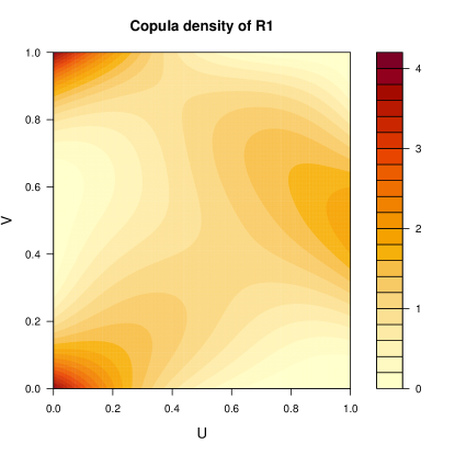
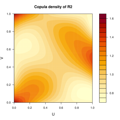
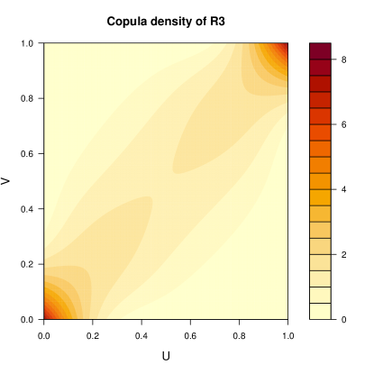
Figure 1: The copula densities with $R_{1},\ R_{2}$, and $R_{3}$ (left), and corresponding randomly generated data (right).

To examine the effectiveness of the methods in Section 3, we conduct three simulation studies. The first simulation study allows us to ascertain conditions under which the penalization is necessary and, using some examples, we also demonstrate the convergence of the algorithm for the penalized log-likelihood functions. The second study illustrates the performance of the cross-validation procedure for choosing tuning parameters, and the third study compares and contrasts methods of model selection including the cross-validation and AIC methods.

4.1 Conditions under which penalization is necessary (Simulation Study I)

Given the true parameter matrices $R_{1},R_{2}$, and $R_{3}$, and also using the generated data, we apply the EM method for penalized log-likelihood functions to estimate $\widehat{R}_{1}$, $\widehat{R}_{2}$, and $\widehat{R}_{3}$. For any such estimator $\widehat{R}$ we define the mean-square error (MSE) corresponding to each pair of tuning parameters $(\alpha,\beta)$ as

$$\mbox{MSE}(\widehat{R}\mathchar 24635\relax\;\alpha,\beta)=\frac{1}{J}\sum^{J}_{j=1}\sum_{k,\ell}(\widehat{r}^{(j)}_{k,\ell}(\alpha,\beta)-r_{k,\ell})^{2},$$ (4.1)

where $J=100$, $\alpha\in[0,0.25]$, $\beta\in[2,4.5]$, and each $\widehat{R}^{(j)}(\alpha,\beta)=\big{(}\widehat{r}^{(j)}_{k,\ell}(\alpha,\beta)\big{)}$ is obtained from the EM method with penalization for given $(\alpha,\beta)$ and data set $j$, where $j=1,\ldots,J$. Following (4.1), we calculate the mean-square errors $\mbox{MSE}(\widehat{R}\mathchar 24635\relax\;\alpha,\beta)$ for 15 equally spaced values of $\alpha$ and 10 equally spaced values of $\beta$, so that 150 MSEs are obtained for each $R_{i}$, $i=1,2,3$.

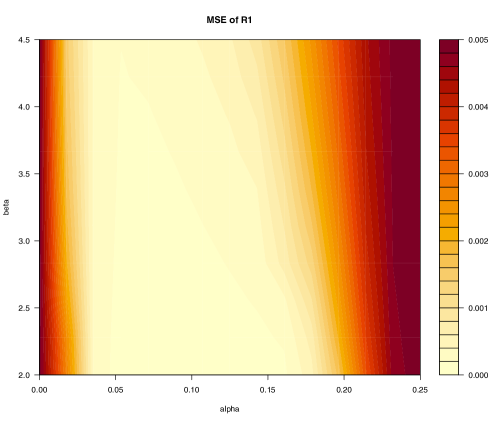
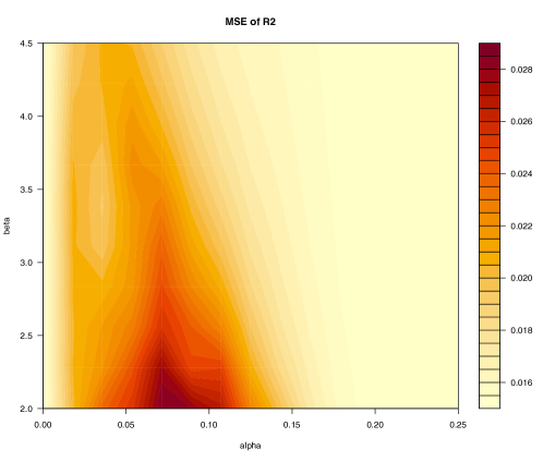
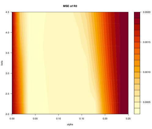
Figure 2: Horizontal axis is $\alpha\in[0,0.25]$, vertical axis is $\beta\in[2,4.5]$. Contour plots of MSEs in (4.1) of $\widehat{R}_{1}$, $\widehat{R}_{2}$ and $\widehat{R}_{3}$ for tuning parameters $(\alpha,\beta)$.

The MSEs of $\widehat{R}_{1}$, $\widehat{R}_{2}$, and $\widehat{R}_{3}$ for different pairs of $(\alpha,\beta)$ are shown in Figure 2 from top to bottom, respectively. We see that the MSEs of $\widehat{R}_{1}$ and $\widehat{R}_{3}$ are large when $\alpha$ is close to $0$ or greater than $0.2$; and the MSE is small when $0.05<\alpha<0.2$. However, the MSE of $\widehat{R}_{2}$ shows a contrary image, which indicates that it is the extreme values of $\alpha$ that will lead to good estimation of $R_{2}$. In other words, when the true parameter matrix $R$ is sparse, penalization is necessary and a properly chosen $\alpha>0$ can lead to better estimation of $R$; on the other hand, if $R$ is not sparse then the EM algorithm without penalization is generally superior.

We also note that the variability of the observed MSEs in the horizontal ($\alpha$) direction is larger than the variability in the vertical ($\beta$) direction. This phenomenon is due to the fact that, in the penalty function, the parameter $\alpha$ is a more essential tuning parameter than $\beta$.

4.2 Convergence properties of the EM algorithm (Simulation Study I)

With three examples of the simulation data sets in Simulation Study I, we illustrate the performance and the convergence properties of the EM algorithm.

The graphs on the left side of Figure 3 show monotonically increasing convergence of the average penalized pseudo-log-likelihood functions (3.5) when the algorithm is applied to each data set. As (3.5) also depends on the values of $(\alpha,\beta)$ then we have in each panel a group of 15 sets of penalized log-likelihood curves, and each group has 10 curves, for the $\alpha$’s and $\beta$’s, respectively.

As expected, when $\alpha=0$, the log-likelihood function attains its highest value; and as $\alpha$ increases, the penalized log-likelihood function takes large decreases in value. That is, each group of curves corresponds to a single value of $\alpha$, and increases in the value $\alpha$ leads to substantially smaller values of the penalized log-likelihood function. For the cases in which $\alpha=0$ or $\alpha\geq\max\{r_{k,\ell}\}$, since $L_{p}(R)=L_{p}^{*}(R)-\mbox{constant}$, we see that the top ($\alpha=0$) and bottom ($\alpha\geq\max\{r_{k,\ell}\}$) lines in each left panel of Figure 3 behave similarly.

For fixed $\alpha$, each group of curves indicate that changes in the value of $\beta$ lead only to minor changes in the values of the penalized log-likelihood function. This phenomenon again implies that the choice of $\alpha$ is more crucial to the penalized log-likelihood function than the choice of $\beta$. Further, it is also evident from these graphs that the EM algorithm maximizes the penalized log-likelihood in each case and without any difficulty.

For the same data sets, the graphs on the right-hand side of Figure 3 illustrate the behaviors of (3.6), the mean of the pseudo-log-likelihood functions for the 150 pairs of $(\alpha,\beta)$. For $0<\alpha<\max\{r_{k,\ell}\},\ k=1,\ldots,m,\ \ell=1,\ldots,n$, we see that the EM method enables (3.6) to attain its maximum value at early stages of convergence. However, the pseudo-log-likelihood function subsequently may decrease temporarily before attaining convergence. Nevertheless the EM algorithm without penalization, i.e., for the case in which $\alpha=0$, continues to increase and convergence is attained perhaps at a slow pace, as shown in the thick black line.

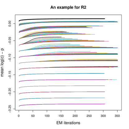
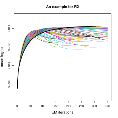
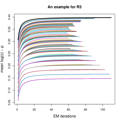
Figure 3: Horizontal axis is the number of EM iterations. Vertical axis is for (3.5) or (3.6) of three data sets. Left: convergence of (3.5) for different pairs of $(\alpha,\beta)$; Right: convergence of (3.6) for different pairs of $(\alpha,\beta)$.

4.3 Choosing the tuning parameters (Simulation Study II)

In the second simulation study, we evaluate the cross-validation method in Section 3.3 for the tuning parameters $(\alpha,\beta)$. Because of the time-consuming nature of cross-validation, we consider reduced sets of $\alpha$ and $\beta$, with $\alpha\in\{0,0.02,0.05,0.1,0.15,0.2,0.25\}$ and $\beta\in\{2,3,3.7,4\}$. For each $R_{i}$, $i=1,2,3$, we use the same $J=100$ sets of random data of size 1,000 as in the first simulation. For each data set $j,\ j=1,\ldots J$, we calculate $CV_{j}(\alpha,\beta\mathchar 24635\relax\;m,n)$ by (3.11), and then we calculate the arithmetic mean of the $CV_{j}$,

$$\overline{CV}(\alpha,\beta\mathchar 24635\relax\;m,n)=\frac{1}{J}\sum^{J}_{j=1}CV_{j}(\alpha,\beta\mathchar 24635\relax\;m,n).$$ (4.2)

The contour plots of $\overline{CV}(\alpha,\beta\mathchar 24635\relax\;m,n)$ are graphed in Figure 4.

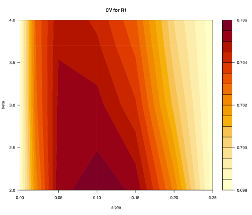
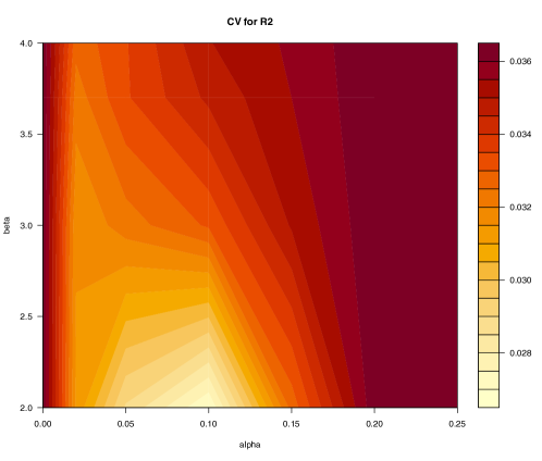
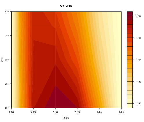
Figure 4: Horizontal axis is $\alpha\in\{0,0.02,0.05,\allowbreak 0.1,0.15,0.2,0.25\}$, vertical axis is $\beta\in\{2,3,3.7,4\}$. Contour plots of average $\overline{CV}(\alpha,\beta\mathchar 24635\relax\;m,n)$ in (4.2) for pairs of $(\alpha,\beta)$.

Since a larger value of $\overline{CV}(\alpha,\beta\mathchar 24635\relax\;m,n)$ indicates superior model fit, we see that the results of Simulation Study II are consistent with the results of Simulation Study I. That is, in the top and bottom panels for $R_{1}$ and $R_{3}$, respectively, for moderate values of $\alpha$, such as $0.05<\alpha<0.2$, cross-validation results in larger values of $\overline{CV}$; as $\alpha$ approaches zero or larger than 0.2, we see that $\overline{CV}(\alpha,\beta\mathchar 24635\relax\;m,n)$ decreases. This means that $\alpha\in(0.05,0.2)$ provides better estimates for $R_{1}$ and $R_{3}$. On the other hand, in the case of $R_{2}$, where no zero elements are contained in the parameter matrix, $\alpha=0$ and $\alpha>0.2$ give larger values of average $CV$ than those in the center. This also suggests that no penalization is necessary in estimating $R_{2}$. Therefore we infer from this study and the related graphs that the cross-validation method with (3.10) is effective for tuning parameter selection and is able to choose $(\alpha,\beta)$ accurately.

4.4 Model selection (Simulation Study III)

In this subsection, we use simulations to examine the performance of the cross-validation and AIC approaches to determining the size of the parameter matrix $R$. For selecting $(m,n)$ we set $\alpha=0$, for simplicity, and we also recall the monotonic increasing property of (3.6) when $\alpha=0$. With this choice of $\alpha$, the parameter $\beta$ becomes extraneous, so we will use the notation $CV(m,n)$ as shorthand for $CV(\alpha,\beta\mathchar 24635\relax\;m,n)$. For each $R_{i}$, $i=1,2,3$, with $d=3$, and equally-spaced interior knots of B-spline basis functions, we generate $J=100$ data sets, each of sample size 1,000 as before.

Using the $j$th data set, we calculate (3.11) for each pair of integers $(m,n)$; thus we obtain $CV_{j}(m,n)$, $j=1,\ldots,J$, and then we compute the mean and standard derivation of all $CV_{j}(m,n)$. We also define $AIC_{j}(m,n)$, the value of the AIC obtained by applying (3.12) to the $j$th data set, $j=1,\ldots,J$, and then we calculate the mean and standard derivation of all $AIC_{j}(m,n)$. The computed results for $m,n\in\{4,5,6,7,8\}$ are given in Tables 1–6.

Table 1: Mean and standard deviation of $CV(m,n)$ for $R_{1}$

$m\,\backslash\,n$		4	5	6	7	8
4	mean	0.518	0.698	0.685	0.685	0.679
	s.d.	0.042	0.075	0.071	0.076	0.078
5	mean	0.551	0.690	0.674	0.668	0.660
	s.d.	0.048	0.075	0.077	0.077	0.078
6	mean	0.550	0.679	0.664	0.655	0.647
	s.d.	0.050	0.077	0.080	0.082	0.084
7	mean	0.556	0.674	0.656	0.645	0.637
	s.d.	0.053	0.077	0.080	0.083	0.083
8	mean	0.551	0.668	0.646	0.635	0.623
	s.d.	0.055	0.078	0.082	0.084	0.084

Table 2: Mean and standard deviation of $CV(m,n)$ for $R_{2}$

$m\,\backslash\,n$		4	5	6	7	8
4	mean	0.039	0.036	0.030	0.023	0.017
	s.d.	0.028	0.030	0.032	0.033	0.033
5	mean	0.032	0.024	0.015	0.006	-0.003
	s.d.	0.030	0.033	0.036	0.036	0.038
6	mean	0.025	0.014	0.003	-0.008	-0.019
	s.d.	0.030	0.033	0.035	0.038	0.040
7	mean	0.020	0.008	-0.006	-0.019	-0.030
	s.d.	0.032	0.034	0.036	0.040	0.041
8	mean	0.014	0.000	-0.016	-0.030	-0.045
	s.d.	0.036	0.036	0.040	0.043	0.045

Table 3: Mean and standard deviation of $CV(m,n)$ for $R_{3}$

$m\,\backslash\,n$		4	5	6	7	8
4	mean	1.585	1.585	1.687	1.680	1.684
	s.d.	0.081	0.081	0.102	0.098	0.103
5	mean	1.585	1.781	1.774	1.772	1.765
	s.d.	0.081	0.115	0.112	0.114	0.116
6	mean	1.685	1.775	1.758	1.755	1.747
	s.d.	0.099	0.112	0.114	0.115	0.115
7	mean	1.678	1.771	1.754	1.747	1.738
	s.d.	0.097	0.115	0.115	0.116	0.115
8	mean	1.680	1.764	1.745	1.735	1.726
	s.d.	0.102	0.118	0.117	0.119	0.120

Table 4: Mean and standard deviation of $AIC(m,n)$ for $R_{1}$

$m\,\backslash\,n$		4	5	6	7	8
4	mean	-195.15	-261.39	-254.19	-254.17	-250.97
	s.d.	16.08	27.98	26.68	28.32	28.93
5	mean	-203.70	-255.60	-251.04	-248.10	-243.62
	s.d.	18.16	27.63	28.78	29.00	29.03
6	mean	-201.15	-251.18	-245.44	-241.23	-235.69
	s.d.	18.65	28.61	29.61	29.94	29.90
7	mean	-200.61	-246.12	-239.36	-233.97	-227.18
	s.d.	19.67	28.67	29.21	29.77	29.80
8	mean	-196.64	-240.96	-232.95	-226.38	-218.10
	s.d.	19.90	28.60	29.14	29.36	29.32

Table 5: Mean and standard deviation of $AIC(m,n)$ for $R_{2}$

$m\,\backslash\,n$		4	5	6	7	8
4	mean	-12.43	-11.38	-8.13	-4.93	-1.39
	s.d.	8.82	9.71	10.09	10.30	10.28
5	mean	-9.61	-7.04	-2.99	1.50	5.91
	s.d.	9.34	10.11	10.51	10.79	10.82
6	mean	-6.27	-2.69	2.51	8.19	13.74
	s.d.	9.54	10.29	10.79	11.19	11.50
7	mean	-2.87	1.63	8.04	14.86	21.46
	s.d.	9.84	10.50	10.84	11.29	11.43
8	mean	0.54	6.19	13.81	21.88	29.94
	s.d.	10.34	10.86	11.65	11.97	12.40

Table 6: Mean and standard deviation of $AIC(m,n)$ for $R_{3}$

$m\,\backslash\,n$		4	5	6	7	8
4	mean	-615.98	-610.00	-647.05	-638.55	-638.62
	s.d.	32.40	32.40	40.05	38.44	40.32
5	mean	-610.01	-686.51	-676.60	-674.80	-669.65
	s.d.	32.40	44.68	43.24	44.69	44.88
6	mean	-646.23	-676.93	-671.97	-666.42	-659.84
	s.d.	39.14	43.39	45.02	45.21	45.04
7	mean	-638.16	-674.47	-666.53	-659.31	-651.77
	s.d.	37.94	44.82	45.18	45.31	45.33
8	mean	-637.29	-669.25	-659.59	-651.06	-642.17
	s.d.	39.62	45.65	45.56	46.05	46.09

From the results given in these tables, we see that both the cross-validation and AIC approaches are useful for selecting $(m,n)$. For $R_{1}$ and $R_{3}$, with help of these methods, we easily detect the correct choices of $(m,n)$. In the case of $R_{2}$, both methods prefer $(m,n)=(4,4)$; however the values of $CV$ and $AIC$ for the second-best model, $(m,n)=(4,5)$, are close to the best and are much closer than all others values of $(m,n)$. Consequently, we may choose either $(m,n)=(4,4)$ or $(m,n)=(4,5)$ for $R_{2}$.

5 An illustrative example

This section presents an application of the proposed methods using birth and death rate data available at the website of “Our World in Data.” The data for year 2021 in Figure 5 pertain to 237 countries, and both the birth and death rates are given per 1,000 people of each country’s population. The marginal densities and distribution functions of the birth and death rates are estimated by the kernel method and by the empirical cumulative distribution function, and the estimates are graphed in Figure 6.

Figure 5: Scatterplot of the data set, birth and death rate

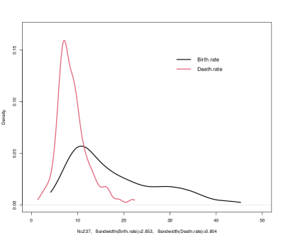
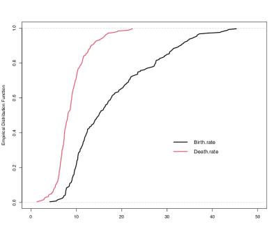
Figure 6: Marginal density functions and empirical cumulative distribution functions

Table 7: AIC values for $(m,n)$

$m\,\backslash\,n$	4	5	6	7	8
4	2798.83	2801.61	2803.66	2806.44	2809.85
5	2798.30	2799.45	2803.99	2810.09	2812.34
6	2798.61	2803.97	2809.58	2816.60	2821.65
7	2801.68	2806.98	2814.28	2822.04	2826.92
8	2805.92	2812.86	2821.63	2831.12	2835.92

Table 8: CV values for $(m,n)$

$m\,\backslash\,n$	4	5	6	7	8
4	0.457	0.445	0.447	0.440	0.435
5	0.525	0.521	0.496	0.451	0.469
6	0.501	0.480	0.419	0.380	0.408
7	0.526	0.442	0.404	0.332	0.449
8	0.508	0.431	0.385	0.272	0.386

By calculating the AIC and carrying out cross-validation for the size $(m,n)$ of the parameter matrix, we obtain the results in Tables 7 and 8. We observe that the AIC attains its minimum at $(m,n)=(5,4)$. However the cross-validation method causes us to hesitate because it provides two competitive larger values at $(m,n)=(7,4)$ and $(m,n)=(5,4)$.

Thus, let us consider the case $(m,n)=(5,4)$. We depict in Figure 7 the results of a five-fold cross-validation study to choose the tuning parameters, i.e., with $M=5$ in (3.11); from that study, we find that $(\widehat{\alpha},\widehat{\beta})=(0.03,2.7)$ from the combinations of $(\alpha,\beta)$ where

$$\alpha \in\{0,0.01,0.02,0.03,0.04,0.05,0.08,0.1,0.12,0.15,0.18,0.20\}$$

$$\beta \in\{2.1,2.2,2.3,2.7,3.0,3.3,3.7,4.0,4.3,4.7,5.0,6.0\}.$$

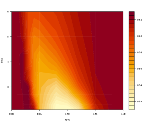
Figure 7: $CV(\alpha,\beta\mathchar 24635\relax\;m=5,n=4)$ of a 5-fold cross-validation for the birth and death rate data

The EM algorithm for the penalized log-likelihood function provides for $R$ the estimate

$$\widehat{R}=\begin{pmatrix}0.007&0.019&0&0.099\\ 0&0&0.099&0.150\\ 0.110&0.111&0.029&0\\ 0.133&0.117&0&0\\ 0&0.003&0.122&0\end{pmatrix}.$$

We present in Figure 8 the corresponding estimated copula density as well as a scatterplot of the empirical cumulative distribution function values of the data $(u_{t},v_{t})$, $t=1,\ldots,237$, calculated by (3.1). Also, the joint density of the data is shown in Figure 9.

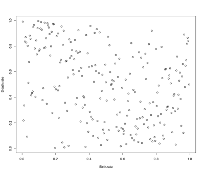
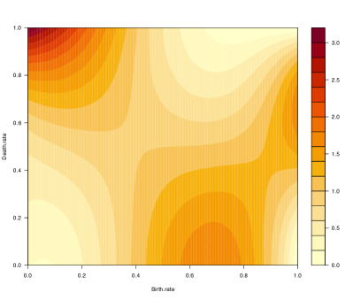
Figure 8: Empirical cumulative distribution function of each data point and the estimated copula density

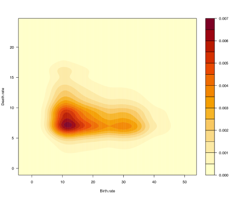
Figure 9: Joint density function of the data

6 Discussion

In this article, we have proposed the EM algorithm for penalized log-likelihood objective functions to estimate the parameter matrix of the B-spline copula. To determine the size of the parameter matrix and the tuning parameters, we provided a new model of $CV$. By means of simulations, we see that the penalized method achieves good performance when the parameter matrix is sparse. We have observed that the non-penalized EM algorithm is superior when there are no zeros in the parameter matrix, and in that case, by setting the tuning parameter $\alpha$ equal to $0$, we can change the EM algorithm to being non-penalized. We also showed that the cross-validation method can choose appropriate tuning parameters for the penalty function and further, that the cross-validation and AIC approaches are useful in model selection.

Acknowledgments

The authors thank Benjamin Poignard of Osaka University for his valuable discussion and advice on this work during the Workshop on Copula Theory in the Institute of Statistical Mathematics, 2022. This work was supported by Waseda University Grants for Special Research Projects (2022R-048).

Appendix A Proofs of Propositions 3.1 and 3.2

To prove the propositions, we first provide the following notation. Let $w$ denote the complete data; that is, $w$ consists of the observed data set $(\mbox{\boldmath{$u$}},\mbox{\boldmath{$v$}})=(u_{t},v_{t})_{t=1,\ldots,N}$ (referred to as the incomplete data), and the label $\tau_{t}\in\{1,\ldots,m\}\times\{1,\ldots,n\}$, $t=1,\ldots,N$, indicating the B-spline basis to which the $t$-th individual belongs (referred to as the missing data).

The likelihood function for the given incomplete data is

$$g(\mbox{\boldmath{$u$}},\mbox{\boldmath{$v$}}\mathchar 24635\relax\;R)=\left\{\prod^{N}_{t=1}\sum^{m}_{k=1}\sum^{n}_{\ell=1}r_{k,\ell}\phi_{k,m}(u_{t})\psi_{\ell,n}(v_{t})\right\}^{1/N},$$

and the penalty function is

$$\tilde{p}(R)=\sum_{k=1}^{m}\sum_{\ell=1}^{n}p(r_{k,\ell}\mathchar 24635\relax\;\alpha,\beta).$$

Then the penalized likelihood is

$$\tilde{g}(\mbox{\boldmath{$u$}},\mbox{\boldmath{$v$}}\mathchar 24635\relax\;R) =g(\mbox{\boldmath{$u$}},\mbox{\boldmath{$v$}}\mathchar 24635\relax\;R)\,\exp(-\tilde{p}(R))$$

$$=\bigg{[}\prod^{N}_{t=1}\sum^{m}_{k=1}\sum^{n}_{\ell=1}r_{k,\ell}\phi_{k,m}(u_{t})\psi_{\ell,n}(v_{t})\bigg{]}^{1/N}\exp\bigg{[}-\sum_{k,\ell}p(r_{k,\ell}\mathchar 24635\relax\;\alpha,\beta)\bigg{]}.$$

Denote by $g_{c}(\mbox{\boldmath{$w$}}\mathchar 24635\relax\;R)$ the likelihood function for the full data set; then the likelihood of the complete data is

$$\tilde{g}_{c}(\mbox{\boldmath{$w$}}\mathchar 24635\relax\;R)=g_{c}(\mbox{\boldmath{$w$}}\mathchar 24635\relax\;R)\,\exp(-\tilde{p}(R)).$$

The conditional likelihood of $w$ given $(\mbox{\boldmath{$u$}},\mbox{\boldmath{$v$}})$ is obtained as

$$k(\mbox{\boldmath{$w$}}|\mbox{\boldmath{$u$}},\mbox{\boldmath{$v$}}\mathchar 24635\relax\;R)=\frac{\tilde{g}_{c}(\mbox{\boldmath{$w$}}\mathchar 24635\relax\;R)}{\tilde{g}(\mbox{\boldmath{$u$}},\mbox{\boldmath{$v$}}\mathchar 24635\relax\;R)}=\frac{g_{c}(\mbox{\boldmath{$w$}}\mathchar 24635\relax\;R)}{g(\mbox{\boldmath{$u$}},\mbox{\boldmath{$v$}}\mathchar 24635\relax\;R)}.$$

The penalized log-likelihood of the incomplete data $L_{p}(R)$ in (3.5) can be rewritten as

$$L_{p}(R) =\log g(\mbox{\boldmath{$u$}},\mbox{\boldmath{$v$}}\mathchar 24635\relax\;R)-\tilde{p}(R)$$

$$=\log\tilde{g}(\mbox{\boldmath{$u$}},\mbox{\boldmath{$v$}}\mathchar 24635\relax\;R)$$

$$=\log\tilde{g}_{c}(\mbox{\boldmath{$w$}}\mathchar 24635\relax\;R)-\log k(\mbox{\boldmath{$w$}}|\mbox{\boldmath{$u$}},\mbox{\boldmath{$v$}}\mathchar 24635\relax\;R).$$ (A.1)

Let $R^{(s)}$ be the parameter matrix used in the $s$-th iteration of the EM algorithm, $\tilde{Q}(R\mathchar 24635\relax\;R^{(s)})$ be the expectation of the penalized log-likelihood of the complete data for $R^{(s)}$, and $H(R\mathchar 24635\relax\;R^{(s)})$ be the expectation of conditional log-likelihood of the complete data given $(\mbox{\boldmath{$u,\mbox{\boldmath{$v$}}$}})$ and $R^{(s)}$. Taking expectations in (A.1), we obtain

$$L_{p}(R) =E_{R^{(s)}}\left[\log\tilde{g}_{c}(\mbox{\boldmath{$w$}}\mathchar 24635\relax\;R)|(\mbox{\boldmath{$u,\mbox{\boldmath{$v$}}$}})\right]-E_{R^{(s)}}\left[\log k(\mbox{\boldmath{$w$}}|(\mbox{\boldmath{$u$}},\mbox{\boldmath{$v$}})\mathchar 24635\relax\;R)|(\mbox{\boldmath{$u$}},\mbox{\boldmath{$v$}})\right]$$

$$=\tilde{Q}(R\mathchar 24635\relax\;R^{(s)})-H(R\mathchar 24635\relax\;R^{(s)}).$$

Proof: [Proof of Proposition 3.1] Let $R^{(\infty)}$ be the maximizer of $\tilde{Q}(R\mathchar 24635\relax\;R^{(s)})$. Then

$$0 =\frac{\partial}{\partial R}\tilde{Q}(R\mathchar 24635\relax\;R^{(\infty)})\bigg{|}_{R=R^{(\infty)}}$$

$$=E_{R}\left[\frac{\partial}{\partial R}\log\tilde{g}_{c}(\mbox{\boldmath{$w$}}\mathchar 24635\relax\;R)|(\mbox{\boldmath{$u$}},\mbox{\boldmath{$v$}})\right]\bigg{|}_{R=R^{(\infty)}}$$

$$=E_{R}\left[\frac{\partial}{\partial R}\log\left\{\tilde{g}(\mbox{\boldmath{$u$}},\mbox{\boldmath{$v$}}\mathchar 24635\relax\;R)+\log k(\mbox{\boldmath{$w$}}|\mbox{\boldmath{$u$}},\mbox{\boldmath{$v$}}\mathchar 24635\relax\;R)\right\}|(\mbox{\boldmath{$u$}},\mbox{\boldmath{$v$}})\right]\bigg{|}_{R=R^{(\infty)}}$$

$$=\frac{\partial}{\partial R}\log\tilde{g}(\mbox{\boldmath{$u$}},\mbox{\boldmath{$v$}}\mathchar 24635\relax\;R)\bigg{|}_{R=R^{(\infty)}}+E_{R}\left[\frac{\partial}{\partial R}\log k(\mbox{\boldmath{$w$}}|\mbox{\boldmath{$u$}},\mbox{\boldmath{$v$}}\mathchar 24635\relax\;R)|(\mbox{\boldmath{$u$}},\mbox{\boldmath{$v$}})\right]\bigg{|}_{R=R^{(\infty)}}.$$

The second expression in the above equation is

$$E_{R}\bigg{[}\frac{\partial}{\partial R}\log k(\mbox{\boldmath{$w$}}|\mbox{\boldmath{$u$}},\mbox{\boldmath{$v$}}\mathchar 24635\relax\;R)|(\mbox{\boldmath{$u$}},\mbox{\boldmath{$v$}})\bigg{]}\bigg{|}_{R=R^{(\infty)}}$$

$$= \int_{\mathcal{W}(\mbox{\boldmath{$u$}},\mbox{\boldmath{$v$}})}\frac{\partial}{\partial R}\log k(\mbox{\boldmath{$w$}}|\mbox{\boldmath{$u$}},\mbox{\boldmath{$v$}}\mathchar 24635\relax\;R)\cdot k(\mbox{\boldmath{$w$}}|\mbox{\boldmath{$u$}},\mbox{\boldmath{$v$}}\mathchar 24635\relax\;R)\,dw\bigg{|}_{R=R^{(\infty)}}$$

$$= \frac{\partial}{\partial R}\int_{\mathcal{W}(\mbox{\boldmath{$u$}},\mbox{\boldmath{$v$}})}k(\mbox{\boldmath{$w$}}|\mbox{\boldmath{$u$}},\mbox{\boldmath{$v$}}\mathchar 24635\relax\;R)\,dw\bigg{|}_{R=R^{(\infty)}}=\frac{\partial}{\partial R}1=0.$$

Hence,

$$\frac{\partial}{\partial R}L_{p}(R)\bigg{|}_{R=R^{(\infty)}}=\frac{\partial}{\partial R}\log\tilde{g}(\mbox{\boldmath{$u$}},\mbox{\boldmath{$v$}}\mathchar 24635\relax\;R)\bigg{|}_{R=R^{(\infty)}}=0.$$

The proof now is complete.

Proof: [Proof of Proposition 3.2] For any $s$-th and $(s+1)$-th iterations of the EM algorithm, we consider the difference of their penalized log-likelihoods

$$L_{p} (R^{(s+1)})-L_{p}(R^{(s)})$$

$$=\big{[}\tilde{Q}(R^{(s+1)}\mathchar 24635\relax\;R^{(s)})-\tilde{Q}(R^{(s)}\mathchar 24635\relax\;R^{(s)})\big{]}-\big{[}H(R^{(s+1)}\mathchar 24635\relax\;R^{(s)})-H(R^{(s)}\mathchar 24635\relax\;R^{(s)})\big{]}.$$

Note that the first term on the right hand side satisfies

$$\tilde{Q}(R^{(s+1)}\mathchar 24635\relax\;R^{(s)})-\tilde{Q}(R^{(s)}\mathchar 24635\relax\;R^{(s)})\geq 0,$$

because the EM algorithm is designed to achieve a larger log-likelihood than the previous iteration. Also, the second term equals

$$H( R^{(s+1)}\mathchar 24635\relax\;R^{(s)})-H(R^{(s)}\mathchar 24635\relax\;R^{(s)})$$

$$=E_{R^{(s)}}\left[\log k(\mbox{\boldmath{$w$}}|\mbox{\boldmath{$u$}},\mbox{\boldmath{$v$}}\mathchar 24635\relax\;R^{(s+1)})|(\mbox{\boldmath{$u$}},\mbox{\boldmath{$v$}})\right]-E_{R^{(s)}}\left[\log k(\mbox{\boldmath{$w$}}|\mbox{\boldmath{$u$}},\mbox{\boldmath{$v$}}\mathchar 24635\relax\;R^{(s)})|(\mbox{\boldmath{$u$}},\mbox{\boldmath{$v$}})\right]$$

$$=E_{R^{(s)}}\left[\log\frac{k(\mbox{\boldmath{$w$}}|\mbox{\boldmath{$u$}},\mbox{\boldmath{$v$}}\mathchar 24635\relax\;R^{(s+1)})}{k(\mbox{\boldmath{$w$}}|\mbox{\boldmath{$u$}},\mbox{\boldmath{$v$}}\mathchar 24635\relax\;R^{(s)})}\bigg{|}(\mbox{\boldmath{$u$}},\mbox{\boldmath{$v$}})\right].$$

Since the logarithm function is concave then, by applying Jensen’s inequality, we obtain

$$H(R^{(s+1)}\mathchar 24635\relax\;R^{(s)}) -H(R^{(s)}\mathchar 24635\relax\;R^{(s)})$$

$$\leq\log E_{R^{(s)}}\left[\frac{k(\mbox{\boldmath{$w$}}|\mbox{\boldmath{$u$}},\mbox{\boldmath{$v$}}\mathchar 24635\relax\;R^{(s+1)})}{k(\mbox{\boldmath{$w$}}|\mbox{\boldmath{$u$}},\mbox{\boldmath{$v$}}\mathchar 24635\relax\;R^{(s)})}\big{|}(\mbox{\boldmath{$u$}},\mbox{\boldmath{$v$}})\right]$$

$$= \log\int_{\mathcal{W}(\mbox{\boldmath{$u$}},\mbox{\boldmath{$v$}})}\frac{k(\mbox{\boldmath{$w$}}|\mbox{\boldmath{$u$}},\mbox{\boldmath{$v$}}\mathchar 24635\relax\;R^{(s+1)})}{k(\mbox{\boldmath{$w$}}|\mbox{\boldmath{$u$}},\mbox{\boldmath{$v$}}\mathchar 24635\relax\;R^{(s)})}k(\mbox{\boldmath{$w$}}|\mbox{\boldmath{$u$}},\mbox{\boldmath{$v$}}\mathchar 24635\relax\;R^{(s)})\,dw$$

$$= \log\int_{\mathcal{W}(\mbox{\boldmath{$u$}},\mbox{\boldmath{$v$}})}k(\mbox{\boldmath{$w$}}|\mbox{\boldmath{$u$}},\mbox{\boldmath{$v$}}\mathchar 24635\relax\;R^{(s+1)})\,dw=\log 1=0.$$

Therefore, we obtain

$$L_{p}(R^{(s+1)})\geq L_{p}(R^{(s)}),$$

and since $s$ was chosen arbitrarily then we have proved that the algorithm always results in monotonically increasing values of $L_{p}(R^{(s)})$.

Appendix B Rejection sampling for generating random data from the B-spline copula

Algorithm 3 Generate random data from the B-spline copula

1:Set the degree of the B-spline basis functions to equal $d$, the size of $R$ to equal $m\times n$, and choose equally-spaced interior knots. This determines the basis functions as well as the $q_{k,m}$ and $q^{*}_{\ell,n}$ for each argument $(u,v)$ of the copula $c(u,v\mathchar 24635\relax\;R)$, $u\in[0,1]$, $v\in[0,1]$.

2:Choose a parameter matrix $R$ that satisfies the conditions in (2.5).

3:Calculate $c_{\max}:=\max_{u,v}c(u,v\mathchar 24635\relax\;R)$, the maximum value of $c(u,v\mathchar 24635\relax\;R)$ on $[0,1]\times[0,1]$, and then the scaling parameter is $K=1/c_{\max}$.

4:Generate independent observations, $U$ and $V$, both from the Unif$(0,1)$ distribution and calculate $c(U,V\mathchar 24635\relax\;R)$.

5:Compute $Kc(U,V)$, the rate of choosing such random pairs $(U,V)$.

6:Generate a new random number $S\sim$ Unif$(0,1)$.

7:If $S\leq Kc(U,V)$, then accept $(U,V)$ as a pair of random numbers of $c(u,v\mathchar 24635\relax\;R)$; otherwise reject $(U,V)$ and repeat Steps 4–7.

References

- \bibcommenthead
- Akaike (\APACyear1974) \APACinsertmetastarAkaike74{APACrefauthors}Akaike, H. \APACrefYearMonthDay1974. \BBOQ\APACrefatitleA new look at the statistical model identification A new look at the statistical model identification.\BBCQ \APACjournalVolNumPagesIEEE Transactions on Automatic Control19716–723. \PrintBackRefs\CurrentBib
- Baker (\APACyear2008) \APACinsertmetastarBaker08{APACrefauthors}Baker, R. \APACrefYearMonthDay2008. \BBOQ\APACrefatitleAn order-statistics-based method for constructing multivariate distributions with fixed marginals An order-statistics-based method for constructing multivariate distributions with fixed marginals.\BBCQ \APACjournalVolNumPagesJournal of Multivariate Analysis992312–2327. \PrintBackRefs\CurrentBib
- Cai \BBA Wang (\APACyear2014) \APACinsertmetastarCaiWang14{APACrefauthors}Cai, Z.\BCBT \BBA Wang, X. \APACrefYearMonthDay2014. \BBOQ\APACrefatitleSelection of mixed copula model via penalized likelihood Selection of mixed copula model via penalized likelihood.\BBCQ \APACjournalVolNumPagesJournal of the American Statistical Association109788–801. \PrintBackRefs\CurrentBib
- de Boor (\APACyear1972) \APACinsertmetastardeBoor72{APACrefauthors}de Boor, C. \APACrefYearMonthDay1972. \BBOQ\APACrefatitleOn calculating with B-splines On calculating with B-splines.\BBCQ \APACjournalVolNumPagesJournal of Approximation Theory650–62. \PrintBackRefs\CurrentBib
- de Boor (\APACyear2001) \APACinsertmetastardeBoor01{APACrefauthors}de Boor, C. \APACrefYear2001. \APACrefbtitleA Practical Guide to Splines, Revised edition A Practical Guide to Splines, revised edition. \APACaddressPublisherNew YorkSpringer. \PrintBackRefs\CurrentBib
- Dou \BOthers. (\APACyear2013) \APACinsertmetastarDou-etal13{APACrefauthors}Dou, X., Kuriki, S.\BCBL Lin, G.D. \APACrefYearMonthDay2013. \BBOQ\APACrefatitleDependence structures and asymptotic properties of Baker’s distributions with fixed marginals Dependence structures and asymptotic properties of Baker’s distributions with fixed marginals.\BBCQ \APACjournalVolNumPagesJournal of Statistical Planning and Inference1431343–1354. \PrintBackRefs\CurrentBib
- Dou \BOthers. (\APACyear2016) \APACinsertmetastarDou-etal16{APACrefauthors}Dou, X., Kuriki, S., Lin, G.D.\BCBL Richards, D. \APACrefYearMonthDay2016. \BBOQ\APACrefatitleEM algorithms for estimating the Bernstein copula EM algorithms for estimating the Bernstein copula.\BBCQ \APACjournalVolNumPagesComputational Statistics Data Analysis93228–245. \PrintBackRefs\CurrentBib
- Dou \BOthers. (\APACyear2021) \APACinsertmetastarDou-etal21{APACrefauthors}Dou, X., Kuriki, S., Lin, G.D.\BCBL Richards, D. \APACrefYearMonthDay2021. \BBOQ\APACrefatitleDependence properties of B-spline copulas Dependence properties of B-spline copulas.\BBCQ \APACjournalVolNumPagesSankhyā A83283–311. \PrintBackRefs\CurrentBib
- Fan \BBA Li (\APACyear2001) \APACinsertmetastarFanLi01{APACrefauthors}Fan, J.\BCBT \BBA Li, R. \APACrefYearMonthDay2001. \BBOQ\APACrefatitleVariable selection via nonconcave penalized likelihood and its oracle properties Variable selection via nonconcave penalized likelihood and its oracle properties.\BBCQ \APACjournalVolNumPagesJournal of the American Statistical Association961348–1360. \PrintBackRefs\CurrentBib
- Genest \BOthers. (\APACyear1995) \APACinsertmetastarGenest-etal95{APACrefauthors}Genest, C., Ghoudi, K.\BCBL Rivest, L\BHBIP. \APACrefYearMonthDay1995. \BBOQ\APACrefatitleA semiparametric estimation procedure of dependence parameters in multivariate families of distributions A semiparametric estimation procedure of dependence parameters in multivariate families of distributions.\BBCQ \APACjournalVolNumPagesBiometrika82543–552. \PrintBackRefs\CurrentBib
- Green (\APACyear1990) \APACinsertmetastarGreen90{APACrefauthors}Green, P.J. \APACrefYearMonthDay1990. \BBOQ\APACrefatitleOn use of the EM for penalized likelihood estimation On use of the EM for penalized likelihood estimation.\BBCQ \APACjournalVolNumPagesJournal of the Royal Statistical Society, Series B52443–452. \PrintBackRefs\CurrentBib
- Hastie \BOthers. (\APACyear2009) \APACinsertmetastarHastie-etal09{APACrefauthors}Hastie, T., Tibshirani, R.\BCBL Friedman, J. \APACrefYear2009. \APACrefbtitleThe Elements of Statistical Learning, Data Mining, Inference, and Prediction, 2nd edn. The Elements of Statistical Learning, Data Mining, Inference, and Prediction, 2nd edn. \APACaddressPublisherNew YorkSpringer. \PrintBackRefs\CurrentBib
- Kauermann \BOthers. (\APACyear2013) \APACinsertmetastarKauermann-etal13{APACrefauthors}Kauermann, G., Schellhase, C.\BCBL Ruppert, D. \APACrefYearMonthDay2013. \BBOQ\APACrefatitleFlexible copula density estimation with penalized hierarchical B-splines Flexible copula density estimation with penalized hierarchical B-splines.\BBCQ \APACjournalVolNumPagesScandinavian Journal of Statistics40685–705. \PrintBackRefs\CurrentBib
- Kojadinovic \BBA Yi (\APACyear2022) \APACinsertmetastarKojadinovic-Yi22{APACrefauthors}Kojadinovic, I.\BCBT \BBA Yi, B. \APACrefYearMonthDay2022. \BBOQ\APACrefatitleA class of smooth, possibly data-adaptive nonparametric copula estimators containing the empirical beta copula A class of smooth, possibly data-adaptive nonparametric copula estimators containing the empirical beta copula.\BBCQ \APACjournalVolNumPagesPreprint arXiv:2106.10726. \PrintBackRefs\CurrentBib
- McLachlan \BBA Krishnan (\APACyear2008) \APACinsertmetastarMcLachlan-Krishnan08{APACrefauthors}McLachlan, G.J.\BCBT \BBA Krishnan, T. \APACrefYear2008. \APACrefbtitleThe EM Algorithm and Extensions, 2nd edn. The EM Algorithm and Extensions, 2nd edn. \APACaddressPublisherNew YorkWiley. \PrintBackRefs\CurrentBib
- Nelsen (\APACyear2006) \APACinsertmetastarNelsen06{APACrefauthors}Nelsen, R. \APACrefYear2006. \APACrefbtitleAn Introduction to Copulas, 2nd edn. An Introduction to Copulas, 2nd edn. \APACaddressPublisherNew YorkSpringer. \PrintBackRefs\CurrentBib
- Sancetta \BBA Satchell (\APACyear2004) \APACinsertmetastarSancetta-Satchell04{APACrefauthors}Sancetta, A.\BCBT \BBA Satchell, S. \APACrefYearMonthDay2004. \BBOQ\APACrefatitleThe Bernstein copula and its applications to modeling and approximations of multivariate distributions The Bernstein copula and its applications to modeling and approximations of multivariate distributions.\BBCQ \APACjournalVolNumPagesEconometric Theory20535–562. \PrintBackRefs\CurrentBib
- Segers \BOthers. (\APACyear2016) \APACinsertmetastarSegers-etal16{APACrefauthors}Segers, J., Sibuya, M.\BCBL Tsukahara, H. \APACrefYearMonthDay2016. \BBOQ\APACrefatitleThe empirical beta copula The empirical beta copula.\BBCQ \APACjournalVolNumPagesJournal of Multivariate Analysis15535–51. \PrintBackRefs\CurrentBib
- Shen \BOthers. (\APACyear2008) \APACinsertmetastarShen-etal08{APACrefauthors}Shen, X., Zhu, Y.\BCBL Song, L. \APACrefYearMonthDay2008. \BBOQ\APACrefatitleLinear B-spline copulas with applications to nonparametric estimation of copulas Linear B-spline copulas with applications to nonparametric estimation of copulas.\BBCQ \APACjournalVolNumPagesComputational Statistics Data Analysis523806–3819. \PrintBackRefs\CurrentBib
- Sklar (\APACyear1959) \APACinsertmetastarSklar59{APACrefauthors}Sklar, A. \APACrefYearMonthDay1959. \BBOQ\APACrefatitleFonctions de répartition à dimensions et leurs marges Fonctions de répartition à dimensions et leurs marges.\BBCQ \APACjournalVolNumPagesPublications de l’Institut de Statistique de L’Université de Paris8229–231. \PrintBackRefs\CurrentBib