Stability of traveling waves in a nonlinear hyperbolic system approximating a dimer array of oscillators
Abstract
We study a semilinear hyperbolic system of PDEs which arises as a continuum approximation of the discrete nonlinear dimer array model introduced by Hadad, Vitelli and Alu (HVA) in [HVA17]. We classify the system’s traveling waves, and study their stability properties. We focus on traveling pulse solutions (“solitons”) on a nontrivial background and moving domain wall solutions (kinks); both arise as heteroclinic connections between spatially uniform equilibrium of a reduced dynamical system. We present analytical results on: nonlinear stability and spectral stability of supersonic pulses, and spectral stability of moving domain walls. Our stability results are in terms of weighted norms of the perturbation, which capture the phenomenon of convective stabilization; as time advances, the traveling wave “outruns” the growing disturbance excited by an initial perturbation; the non-trivial spatially uniform equilibria are linearly exponentially unstable. We use our analytical results to interpret phenomena observed in numerical simulations.
Keywords— solitary wave, kink, domain wall, stability and instability of coherent structures
1 Introduction
1.1 Background and motivation
We study the system of semi-linear hyperbolic PDEs:
| (1.1) | ||||
governing the time evolution of . The properties of the nonlinearity, are discussed below in section 1.2. Our study is inspired by work of Hadad, Vitelli and Alu (referred to as HVA in this article) [HVA17], who introduced a nonlinear variant of the discrete and linear Su-Schrieffer-Heeger (SSH) dimer model [ssh79], which can be experimentally realized via an array of coupled nonlinear electrical circuit elements; see (1.7) below. The SSH model is well-known to exhibit topological transitions, related to the closing (and formation of a linear crossing at “Dirac points” in the band structure) and re-opening of a spectral gap in its band structure as the ratio of the intra-cell to inter-cell coupling (hopping) coefficients is varied. HVA studied a continuum model, appropriate for wave-packet excitations centered on the Dirac point quasi-momentum. They derived, via phase portrait analysis and numerics, traveling pulse solutions (solitons) and traveling domain wall solutions (kinks/antikinks). They then studied, by numerical simulations, the spatially discrete nonlinear time-evolution for initial data given by such solitons and kinks, sampled on the lattice. These numerical simulations of the discrete model showed that the core of both kinks and supersonic pulses appears to be stable against small spatially localized perturbations. Extensive simulations of the time-dependent nonlinear continuum model, (1.1) (see [li2023thesis][du2023discontinuous]) demonstrate that this traveling core is convectively stable; the core persists although away from the core the solution tends to grow with advancing time.
In this article, we present analytical results for the system (1.1) on nonlinear stability and spectral stability of supersonic pulses (solitons) that asymptote to different nontrivial equilibria, and spectral stability of moving domain walls (kinks), which contribute to an understanding of the dynamics.
We next present a precise mathematical formulation, discuss numerical results which exhibit the phenomenon of convective stabilization of pulses and solitons, and summarize our analytical results.
1.2 Assumptions on the nonlinearity
Throughout this article, the nonlinearity in (1.1), for , is assumed to be smooth and to satisfy:
-
()
for , and , . 111By , etc., we always mean etc. The parameter
(1.2) will play an important role.
-
()
.
A common physical assumption is that the nonlinearity be saturable. We say that the nonlinearity is saturable if is replaced by
and further that , and its derivatives , , decay to zero sufficiently rapidly as .
An example of a saturable nonlinearity is . An example of a general nonlinearity is .
The system (1.1) is a semilinear hyperbolic system, whose characteristic lines are given by solutions of . Any solution satisfies the conservation law
| (1.3) |
The conservation law (1.3) plays a role in our classification of traveling wave solutions in section 2, and in the proof and application of finite propagation speed in sections 3.2 and section 4. The system (1.1) does not appear to be of Hamiltonian type. It does have certain discrete symmetries which we summarize in the following:
Proposition 1.1 (Discrete Symmetries).
The proof of proposition 1.1 is very straightforward and we omit it.
1.3 Phenomena motivating this work
System (1.1), with nonlinearity assumptions and , has spatially uniform equilibria:
| either or , where ; see . | (1.4) |
In section 2 we classify the traveling wave solutions (TWS) of (1.1), which are of the form
| (1.5) |
and tend to spatially uniform equilibria at infinity:
Here, and are among the spatially uniform states displayed in (1.4). Traveling wave solution profiles, , are heteroclinic orbits in the phase portrait of a two-dimensional dynamical system obtained from (1.1) via the ansatz (1.5); see Section 2.
Pulses are orbits connecting distinct nontrivial equilibria satisfying , and kinks (and antikinks) are those which connect the trivial equilibrium with a non-trivial equilibrium. Pulses may be supersonic () or subsonic (), while kinks and anti-kinks are all subsonic.
1.3.1 Convective stability and weighted spaces
Consider the case of a supersonic pulse with . figure 1 displays snapshots of the time-evolution of a localized perturbation of . This initial perturbation generates time-evolving perturbations of the pulse which, in a frame of reference moving with the traveling wave speed, , appear to travel leftward, away from the traveling pulse core, while also growing in amplitude. In this same moving frame of reference, the deviation from an exact traveling wave profile, when measured within a fixed semi-infinite “window” , tends zero as increases because perturbations exit the window at as increases. We say that the supersonic pulse (or its core) is convectively stable. The notion of convective stability has been considered previously in, for example, [pego1994asymptotic, martel2001asymptotic, pego1997convective].
We capture this stabilization of the traveling wave core by working in weighted function spaces. In a reference frame moving with the traveling wave solution , perturbations are studied as elements of , where the weight is chosen to be of exponential type. Specifically, is monotone and of the form
see section 5.1.1. If, in the moving frame (speed ), the perturbation travels in the direction of decrease of (to the left), then it is registered as decaying with advancing time if the time rate of amplitude growth is not too large. This intuition underlies our nonlinear and spectral stability results for supersonic pulses; see section 1.4.
Remark 1.2 (Do solutions grow without bound in ?).
We note that numerical simulations of the nonlinear PDEs suggest that the perturbation of traveling wave may be growing without bound. (Note that we have no a priori bound on the solution; see Theorem 3.2.) However, as time advances, the perturbation grows in regions which are further and further away from the traveling wave core. This behavior of the perturbation is registered as time-decay with respect to the weighted norm. This convective stability scenario differs from the more typical scenarios in solitary wave stability. For example, in KdV type equations, which are Hamiltonian and come with an a priori bound on the norm, the perturbation remains bounded and is in fact comprised of small amplitude solitary waves and a radiation component which together decay in appropriate weighted or local energy norms; see, for example, [pego1994asymptotic, martel2001asymptotic].
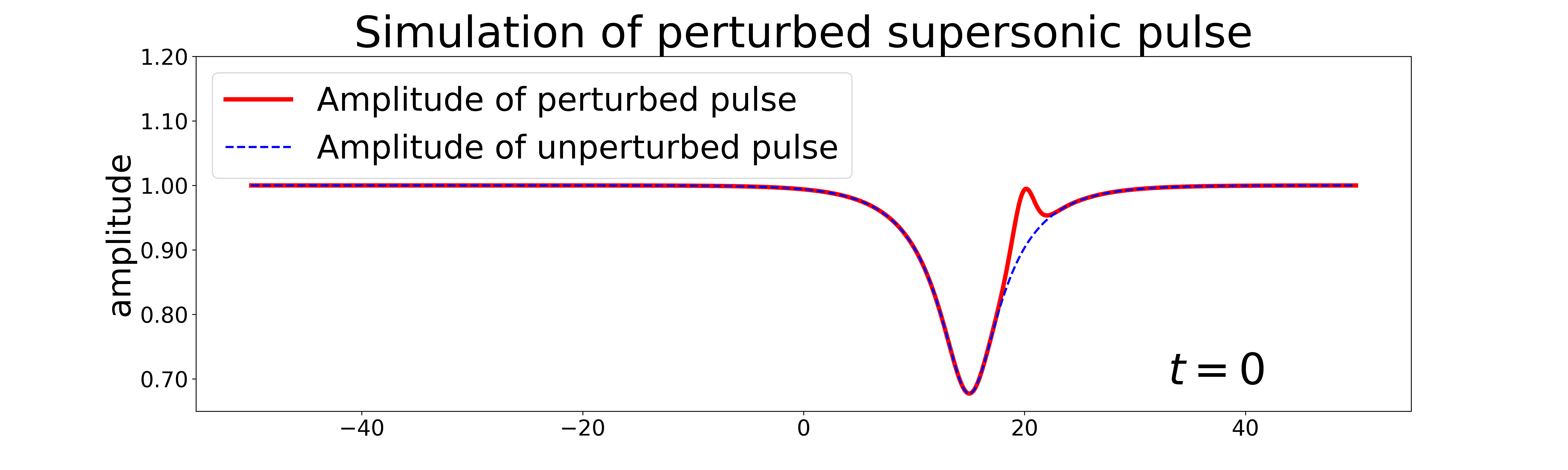
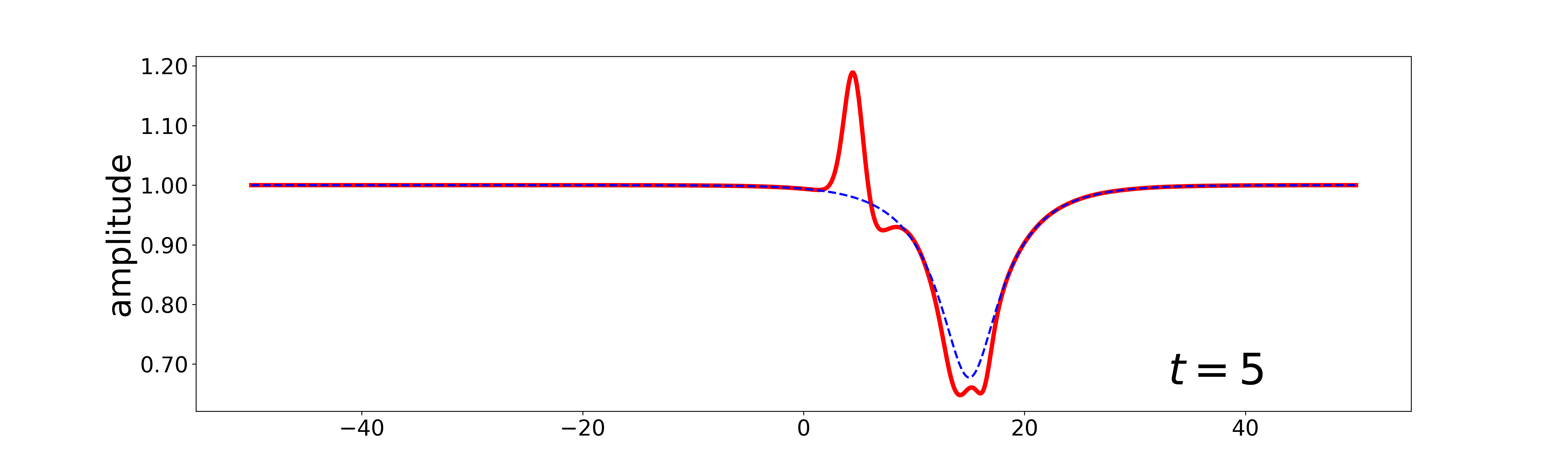
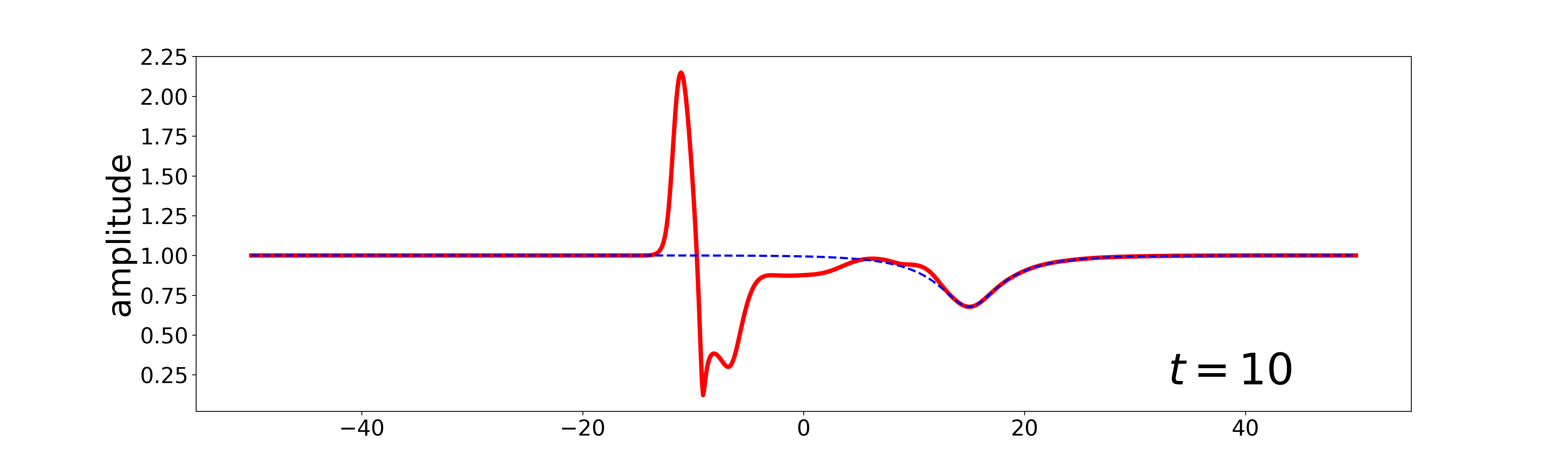
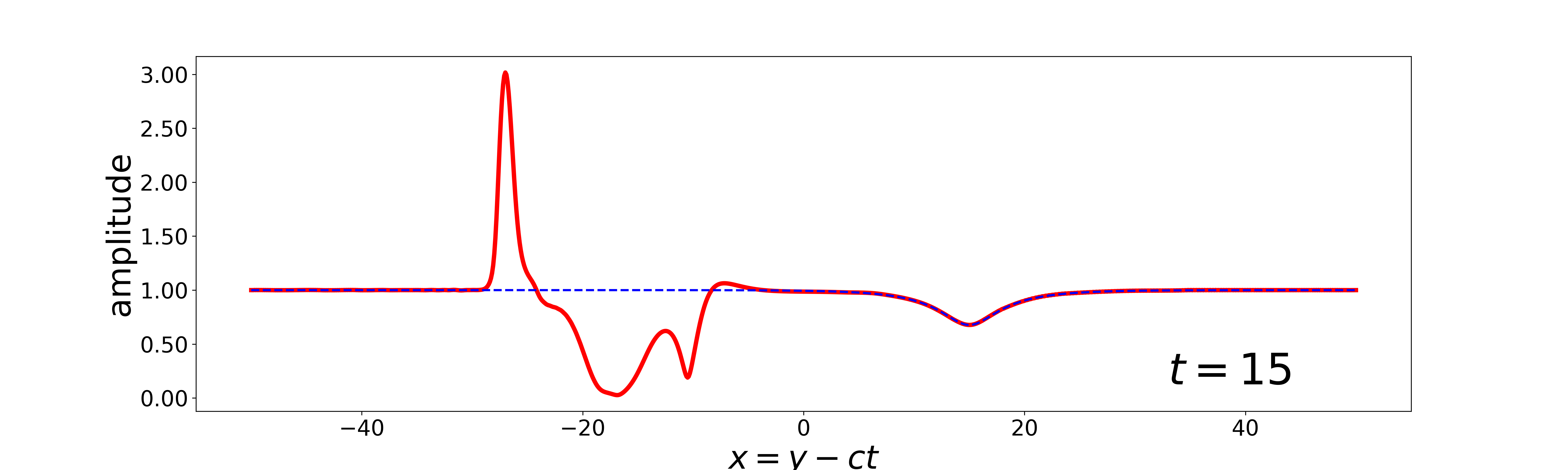
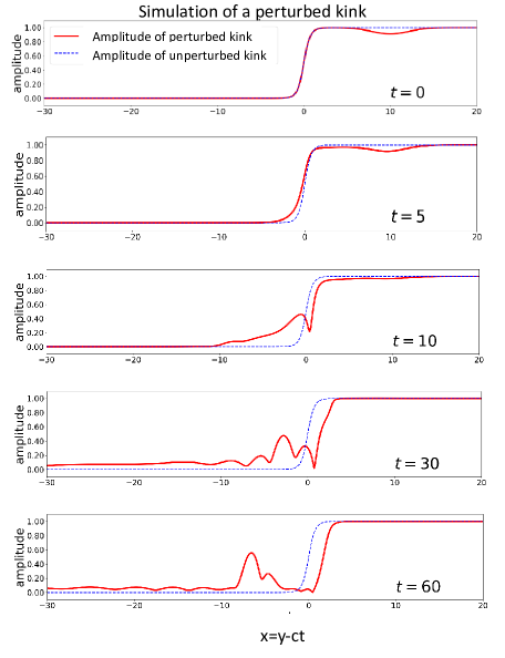
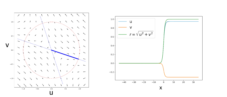
Figure 2 displays numerical simulations illustrating the convective stability of kinks, which are all subsonic (). Here too, we observe in a frame of reference traveling at the same speed as does the unperturbed kink. The kink outruns the generated perturbations as time advances, consistent with our results on linear stability of kinks; see section 1.4 and the discussion of section 1.5.2.
1.4 Summary of results
We summarize the results presented in this article.
- •
- •
- •
- •
1.5 Future directions, open questions
We list some possible directions for future investigation and corresponding open questions.
1.5.1 Large time selection of supersonic pulses problems
Consider a supersonic pulse of speed . Theorem 7.1 on spectral stability and Theorem 4.1 on nonlinear asymptotic stability are convective stability results, which measure the initial perturbation in spatial norms with an exponential weight. The exponential rate satisfies constraints which depend on the underlying traveling wave speed, , and properties of the nonlinearity. In particular, the weighted norm imposes a minimal decay rate of the perturbation in the direction of pulse propagation. What does a supersonic pulse evolve into, under perturbations which violate the decay rate constraints in Theorems 4.1 and 7.1 ?
Note that any supersonic pulse (of speed ) whose profile connects two equilibria on the unit circle, is embedded in a continuous family of supersonic pulses with speeds encompassing the range ; see Figure 7. Further, the profile of a supersonic pulse of speed approaches its asymptotic values at an exponential rate, given in (2.22), which becomes smaller as grows; see Section 2.4.
Does a supersonic pulse traveling with speed , when perturbed by a slow-decaying perturbation – outside the validity of Theorem 4.1 – evolve into a supersonic pulse of some speed , with a compatible spatial decay? If so, what determines the asymptotically selected profile?
1.5.2 Nonlinear stability of kinks
Our spectral stability analysis and numerical simulations (see figure 2) suggest that the family of spatial translates of a kink is nonlinearly convectively stable. We conjecture the following: Let denote a kink and a sufficiently rapidly decaying initial perturbation. Then, there exists , depending on (and ), such that the solution to (2.1) with initial data , satisfies
| (1.6) |
The phase shift in (1.6) is related to the zero energy translation mode of the linearized operator, see Theorem 8.7 and remark 8.8. In contrast, Theorem 4.1 on nonlinear and convective (asymptotic) stability of supersonic pulses, requires no asymptotic phase adjustment. This is corroborated by numerical studies showing no phase shift in the emerging stable supersonic pulse, see figure 1. Note: although there is a state which is formally in the kernel of the linearized operator (due to translation invariance of (1.1)), this state is not in the weighted space with respect to which the supersonic pulse is spectrally stable; see Theorem 7.1 and the discussion following proposition 7.3.
Another question is to clarify the scenario described in Remark 1.2, which is based on numerical simulations. And an example of further technical questions concerning kinks is whether, for example, spectral stability can be established if the concavity assumption () (used in (8.14)), on the nonlinearity, is relaxed.
1.5.3 Alternative measures of the perturbation’s spatial localization and size
Our stability results for pulses (nonlinear and spectral stability) and kinks (spectral stability) are formulated in function spaces, requiring exponential decay of the perturbation in the direction of propagation of the traveling wave. It would be of interest to extend these stability results to spaces with weaker spatial localization requirements; for example, algebraically weighted spaces [miller1997spectral] or [martel2001asymptotic].
1.6 Linear asymptotic stability
For the case of supersonic pulses, we believe that our results on linear spectral stability can be used to obtain exponential time-decay bounds for the linear semi-group , along the lines of the analysis of [pego1994asymptotic, pego1997convective]. For the case of kinks, where the spectrum of is spectrally stable, but with part of its spectrum on the imaginary axis, we expect the governing time decay to be dispersive type, after projecting out the zero energy mode.
1.6.1 Periodic solutions
As discussed in detail in [li2023thesis] (1.1) has rich families of periodic solutions traveling wave solutions. Their stability properties is an open question.
1.6.2 Relation between discrete and continuum models
Finally, system (1.1) is introduced in [HVA17] as a formal continuum approximation for a nonlinear discrete array of coupled nonlinear circuits, valid for excitations whose spatial scale is slow on the inter-dimer length scale. After scaling and nondimensionalization, the discrete system takes the form
| (1.7) | ||||
As demonstrated in[HVA17] there is evidence of the pulse-like and kink-like behaviors in the discrete system (1.7). It is of interest to understand the relation between our continuum analytical and numerical results for (1.1) and those observed, thus far only numerically, in (1.7).
1.7 Notation and conventions
-
1.
denotes the Sobelev space with norm given by:
where denotes the Fourier transform.
-
2.
Weighted spaces: We define the weighted spaces, with weight where is a real-valued function on as
(1.8) for details of the particular weighted spaces used in this work, see Section 5.1.1.
-
3.
Coordinates: The linear stability analysis of this work is always conducted in frames of reference that travel at the speed of an underlying traveling wave. We denote with the spatial coordinate in the non-moving (lab) frame of reference, cf. (1.1), and with the spatial coordinate in the frame of reference traveling with some speed ; see (2.1).
-
4.
Default branch of the square root function: We define function in such a way that its values have non-negative real parts. In particular, and is conformal from the cut complex plane, , to the open right-half plane . For , is continued from above the cut and its values always have non-negative imaginary parts, e.g., .
-
5.
Pauli matrices: We use the standard convention of defining Pauli matrices, and , as a set of basis in the linear space of 2-by-2 complex matrices:
(1.9) Here for and and .
1.8 Acknowledgements
The authors wish to thank A. Alù, Y. Hadad, Q. Du and L. Zhang for many stimulating discussions. This research was supported in part by NSF grant DMS-1908657 (MIW, HL), DMS-1937254 (MIW) and Simons Foundation Math + X Investigator Award # 376319 (MIW, HL). AH was supported in part by the Simons Collaboration on Extreme Wave Phenomena Based on Symmetries and AFSOR Grant No. FA9950-23-1-0144. Part of this research was completed during the 2023-24 academic year, when M.I. Weinstein was a Visiting Member in the School of Mathematics - Institute of Advanced Study, Princeton, supported by the Charles Simonyi Endowment, and a Visiting Fellow in the Department of Mathematics at Princeton University.
2 Traveling wave solutions
We express (1.1) with respect to a coordinate system traveling with speed , where . Setting we obtain
| (2.1) | ||||
For , the system (2.1) has the equilibria:
| (2.2) |
The profile of a traveling wave solution (TWS) profile, , of speed is an orbit of the dynamical system
| (2.3) | ||||
If , we say the TWS is supersonic and if say that it is subsonic.
Evaluating the conservation law (1.3) on a TWS , we conclude that along its phase plane trajectory, the “energy” of :
| (2.4) |
is independent of . Thus, traveling wave profiles correspond to connected subsets of level sets in of :
2.1 Level sets of
-
•
For , is positive definite. Hence, the level sets are ellipses parametrized by :
(2.5) This family of ellipses degenerates to the origin, as .
-
•
For , is negative definite. Hence, the level sets are ellipses parametrized by :
(2.6) This family of ellipses also degenerates to the origin, as .
-
•
For , is indefinite. The level sets are hyperbolas with two branches, with one orientation for and another orientation for . As , and as , these level sets degenerate to a pair of lines which intersect at the origin.
2.2 Bounded heteroclinic traveling wave solutions
We denote a bounded traveling wave solution (TWS) profile with speed for the parameter by . A bounded TWS, , corresponds to a bounded heteroclinic orbit of (2.3) which connect, as varies from to , distinct equilibria which lie in the set:
| (2.7) |
Hence, heteroclinic orbits are determined by the bounded connected subsets of level sets of , whose boundary points lie in the set of equilibria (2.7). See Figures 3-6 222The reduced dynamical system (2.3) also has periodic orbits for ; we do not study these solutions in the present work..
The following proposition, displays relations among traveling wave orbits, which are implied by the symmetries of (1.1).
Proposition 2.1 (Discrete symmetries of the family of traveling wave solutions).
Let be the profile of a TWS with speed . The corresponding solution of (1.1) can be transformed into other TWSs under discrete transformations , and given in proposition 1.1. In particular, the profiles of and corresponding conserved quantity of the transformed traveling wave solution is listed below.
-
(i)
is a TWS with speed whose profile is and .
-
(ii)
is a TWS with speed whose profile is and .
-
(iii)
is a TWS with speed whose profile is and .
Remark 2.2.
N.B. In view of Proposition 2.1 we shall focus, particularly in our stability analyses, on the case of right-moving pulses and kinks, . The linearized spectra of TWSs indeed respect these symmetries; see Theorem 6.2. A complete classification of all traveling wave solutions and their relation through discrete transformations is given in appendix A.
2.3 Traveling Pulses and Domain Walls (Kinks and Anti-kinks)
The set of equilibria (fixed points) of the system (2.3) consists of the origin together with the unit circle of the plane; see (2.7). There are no non-trivial homoclinic orbits – all homoclinic orbits are fixed points/equilibria. However, there are many heteroclinic orbits connecting either distinct points on the unit circle, or some point on the unit circle and the origin. A heteroclinic orbit connecting a pair of fixed points on the unit circle is called a pulse; its amplitude as . A heteroclinic orbit connecting the origin and the unit circle is either a kink or antikink (examples of moving domain walls); tends to as and as (kink) or tends to as and as (antikink).
2.3.1 Pulses: Supersonic and Subsonic
Consider a traveling pulse solution (with speed and energy parameter ) given by a heteroclinic orbit connecting distinct equilibria on the unit circle. If this orbit asymptotes to the equilibrium , then since is constant, we have
| (2.8) |
and hence . It is easy to see that if , then there are four distinct values of in the interval satisfying (2.8). Fix to be the solution of of smallest absolute value. If , then the ellipse intersects the unit circle at the four points
| (2.9a) | ||||
| (2.9b) | ||||
| (2.9c) | ||||
| (2.9d) | ||||
The point is a reflection of the point , and the is a reflection of the point , both with respect to the line . They are distinct points provided and form a pair of double points on this line for . Thus, any and (here with ) gives rise to an ellipse with the four intersection points (2.9). Note: if , then the four points come in pairs which are reflections about the line .
Conversely, given any and , we define via (2.8) and find that
| expressions (2.9), with replaced by , are the intersection points of the ellipse | |||
| (2.10) |
For , the level sets are hyperbolae with two branches in the plane. The branches are both symmetric about or about , and each branch intersects the unit circle at two distinct points, for a total (again) of four intersections.
Supersonic traveling pulses, : For the level set
| (2.11) |
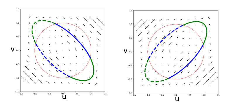
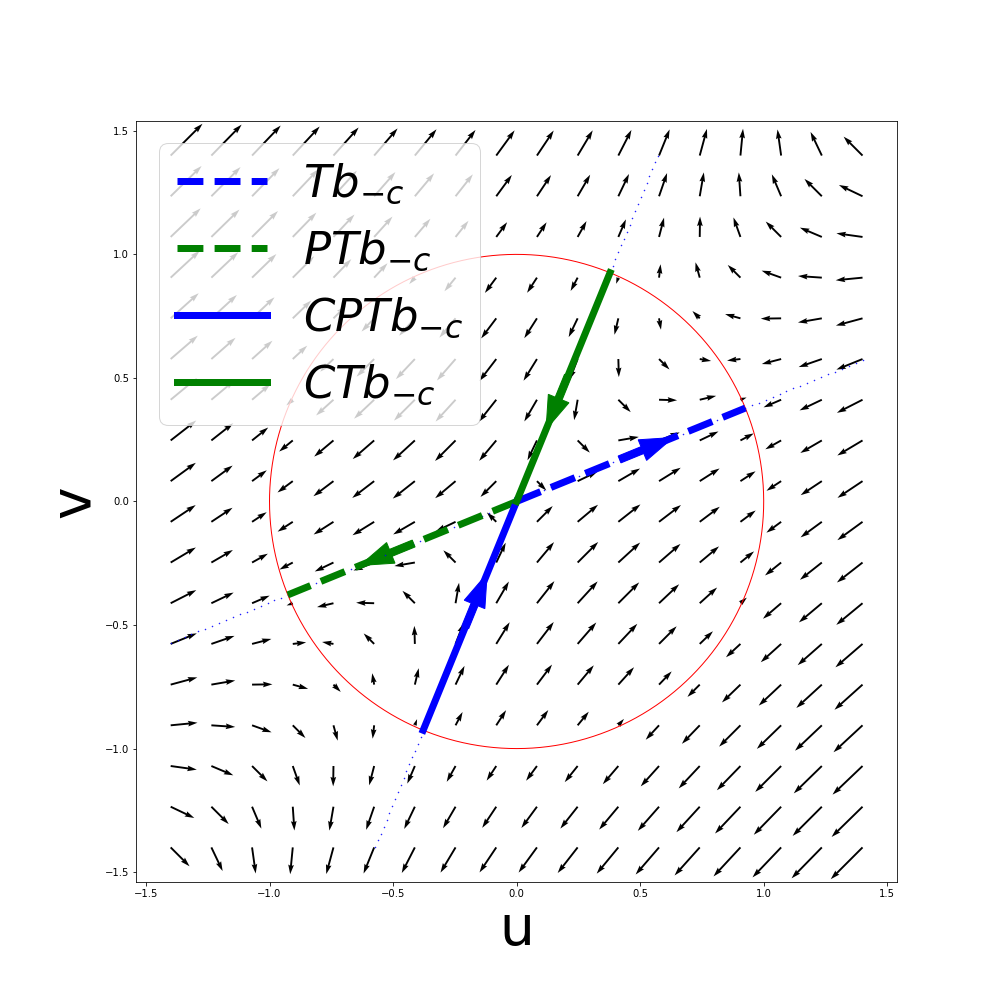
is an ellipse which passes through the four points (2.9) on the unit circle. The portion of this ellipse which is exterior to the unit circle is called a bright soliton pulse, and the portion of this ellipse which is interior to the unit circle is called a dark soliton pulse; see Figure 3. For given and , the orbits corresponding to supersonic pulses with speeds and phase portrait energy parameters can be related to one another via the discrete symmetries displayed in proposition 2.1; see figure 3.
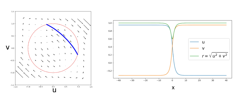
Subsonic traveling pulses, : From the above discussion, for the level set (2.11) is a hyperbola with two branch curves. Each branch curve intersects the unit circle at two points of the points in (2.9). The part of a branch curve contained inside the unit disc is a subsonic dark soliton pulse. The parts of branch curves which lie outside unit disc are unbounded and correspond to spatially unbounded traveling waves; we do not consider these.
2.3.2 Kinks and Antikinks as limits of subsonic pulses
For the case of subsonic () pulses, the hyperbolic level sets, which determine subsonic (dark) pulses, degenerate, as , into two straight lines. For example, if , then by the expression in (2.5), then the limiting two lines are given by:
| (2.12) |
These lines determine four line segments in the phase portrait which connect the origin to a distinct point on the unit circle; see figure 5.
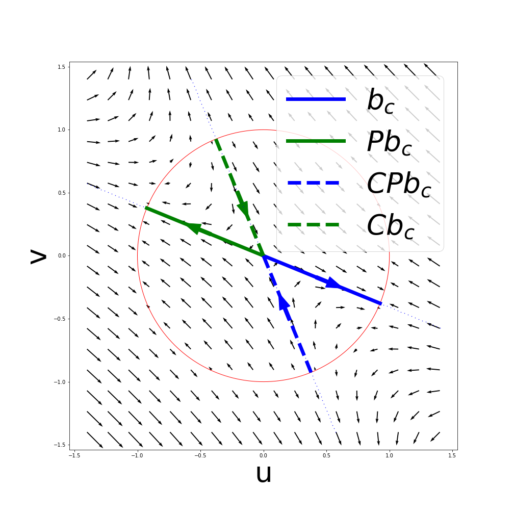
The corresponding four solutions consist of two kinks and two antikinks; those profiles for which the phase portrait trajectory radius approaches the unit circle in the direction of transport () are called kinks, and those for which the approach to the unit circle is in the direction which is opposite to the direction of propagation, are called antikinks. See figure 6 for an example. proposition 2.1 discusses relations among kink and antikink trajectories under discrete symmetry transformations. Along these four kink and antikink trajectories the dynamics (2.3) reduces, thanks to (2.12), to a one dimensional dynamical system of the general form 333Let (), denote the orbit connecting the origin to the unit circle at , with . Its amplitude increases to as : (2.13) where .
2.4 Convergence rate of heteroclinic orbits to asymptotic equilibria
Along a trajectory in the phase portrait, as approaches its asymptotic state on the circle, along its stable manifold. The behavior, near an equilibrium , is characterized by the constant coefficient linearization of (2.3):
| (2.14) |
The matrix in (2.14) has eigenpairs:
| (2.15) | |||
| (2.16) |
We may express the nontrivial eigenvalue of the linearization, in terms of the parameters and . Along a pulse or a kink solution we must have . Hence, and therefore .
For a kink, , from . Therefore, we have for the asymptotic behavior of kink as :
| (2.17) |
and as , for pulses
| (2.18) |
The translation modes has the same exponential decaying behavior, for kinks:
| (2.19) |
and for supersonic pulses
| (2.20) |
Note that the asymptotic behavior does not depend on which of the four non-trivial equilibria (see (2.9)) are approached as tends to infinity.
2.5 Family of supersonic pulses with fixed asymptotics
Consider supersonic pulses with speed , obtained from the ellipse
By the observation (2.10), for fixed , the family of ellipses has the same four intersection points with the unit circle for all . In polar coordinates, , these curves are given by
The minimum radius , is attained at :
| (2.21) |
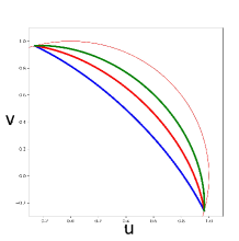
For each there is a traveling wave trajectory, , that connects to ; see Figure 7.
These pulses have different rates of approach to their asymptotic equilibria (see (2.20)) :
| (2.22) |
From (2.21) and (2.22) we see that supersonic pulses corresponding to slower speeds (say , but ) have a deeper dip in their intensity profile () and approach their spatial asymptotes rapidly, while supersonic pulses corresponding to faster speeds (say ) have a shallower dip in their intensity profile and approach their spatial asymptotes slowly.
3 Nonlinear dynamics around traveling wave solutions
Throughout this section, we require the nonlinearity to be saturable; see section 1.2. We derive the hyperbolic system of PDEs (3.2) for
| (3.1) |
the perturbation about a fixed traveling wave solution . We then establish well-posedness of the initial value problem for (3.2); local well-posedness using standard fixed-point techniques and global well-posedness via Grönwall’s inequality applied to integral inequalities for the norm of the solution. We then prove finite propagation speed of information via energy-type arguments. Then, we provide a bound on the growth rate of the perturbations, for an arbitrary initial perturbation. We use this bound, together with our finite propagation speed result, to prove nonlinear convective and asymptotic stability of supersonic pulses, for initial pertubations, , which decay rapidly enough as .
3.1 Local and global well-posedness
Consider (2.1) with initial data which is a perturbation of a TWS: . Writing , we obtain that the perturbation (see (3.1)) solves the initial value problem:
| (3.2) | ||||
where and
| (3.3) |
with initial data . A formally equivalent integral formulation of the IVP is
| (3.4) |
in terms of the semi-group
A solution of (3.4) is called a mild solution of the initial value problem for (3.2). For , Fourier transform with respect to of gives
Therefore is a unitary group on for all by Plancherel’s identity.
To prove our well-posedness results, we require properties of the nonlinearity (see (3.2)), which we summarize in the following proposition. The proof is given in appendix B.
Proposition 3.1.
Assume that in (2.1) is a saturable nonlinearity. Consider the nonlinear mapping given in (3.2). as a mapping only depends on the nonlinearity profile and the TWS . For , the following hold:
-
1.
is globally Lipschitz on . Namely, for any , there is a constant independent , such that
(3.5) -
2.
is locally Lipschitz on . In particular, for any , there is a constant independent of such that
(3.6) As a special case, for any ,
(3.7)
The following global well-posedness result holds:
Theorem 3.2 (Global well-posedness of the mild solution of (3.2)).
For , (3.2) has a unique global mild solution , which satisfies the following exponential bound:
| (3.8) |
The constant depends on and but does not depend on the initial data, .
Proof of Theorem 3.2.
The proof is standard so we only remark briefly on it. Local well-posedness follows from a standard application of contraction mapping principle, whose hypotheses on the nonlinear term, , are verified in proposition 3.1. The key to global well-posedness is the bound (3.8) which we now prove. From (3.4) and estimate (3.7) we have:
Therefore Grönwall’s integral inequality[HuNa01] yields (3.8). Following standard arguments (see, for example, [Reed76, Theorem]), we conclude the global existence of mild solutions to (3.4) in . ∎
3.2 Finite propagation speed
Substitute and in (1.1) (non-moving frame) and we have
| (3.9) | ||||
which governs the perturbation in the non-moving reference frame. For simplicity, we have introduced the notation
| (3.10) |
The following result says the speed of propagation of data for the system (3.2) is at most :
Proposition 3.3.
Consider the initial value problem for the system (3.9) with initial data . Fix and .
-
1.
Assume . If for all , then for all where
(3.11) is called the domain of dependence of the space-time point .
-
2.
Assume are such that for . Then, on .
-
3.
Suppose that for some , for all . Then, for all satisfying we have . In the moving frame with speed where the spatial coordinate is , we have for all .
Proof.
Introduce characteristic variables
| (3.12) |
and
Therefore,
| (3.13) | ||||
Denote a second solution which satisfies (3.9). Analogously we define, via (3.12), . Taking the difference, we obtain coupled equations of and :
| (3.14) | ||||
We next derive an energy inequality from (3.14). Multiply both sides of the first equation of (3.14) with , and similarly the second equation in (3.14) with . Adding the results gives
| (3.15) | ||||
Fix . Assume initial data on , and consider the closed trapezoidal region on the -plane:
| (3.16) |
where . The region is bounded by the four line segments and is shown in figure 8. It is easy to check ; see (3.11).
Integrating (3.18) over and applying Gauss’s divergence theorem we obtain:
| (3.19) | ||||
Now we bound pointwise the absolute value of the integrand on the last line. Note that , are bounded since the TWSs we work with in this paper are all bounded. The derivative of the nonlinearity, , is also bounded since it is continuous, and its arguments are all bounded. By the growth rate bound (3.8) of Theorem 3.2, we have that
on the fixed time interval , the thus the norm of the perturbation is bounded. Moreover,
where the constants depends on the nonlinearity, TWS profile as well as . These estimates imply that the absolute value of the expression on the last line of (3.19) has the upper bound:
Let be the nonnegative function of defined by the third line of (3.19):
Then,
where we used that by the assumption on . By Grönwall’s inequality for . This proves Part 2 of Proposition 3.3.
Part 3 of proposition 3.3 is an immediate consequence of Part 2. To see this, suppose on for some . Now if , then . Hence, for all such , we have for . Thus, for all such that . Equivalently, in a frame of reference moving with speed : . See figure 9 for illustration of this part of the proof. Part 3 is thus proved, and the proof of proposition 3.3 is now complete.
∎
4 Nonlinear convective stability of supersonic pulses
Consider a supersonic pulse, traveling with speed . The following theorem is stated in the comoving frame, i.e., for an “observer” that travels with the pulse at speed . We continue with the assumption that the nonlinearity is saturable as we do for the last section; see section 1.2.
Theorem 4.1 (Supersonic pulses are nonlinearly convectively stable).
Assume a saturable nonlinearity. Let be a supersonic pulse that travels with speed .
-
1.
Consider equation (3.9) for the perturbation in a non-moving frame of reference, with initial data . Assume that for some , if , then
(4.1) Then, for any , we have exponential time-decay:
(4.2) - 2.
In particular, any Gaussian perturbation, , centered at an arbitrary point, satisfies (4.1). Numerical simulations of the evolution, which are consistent with theorem 4.1 are presented in figure 1. Theorem 4.1 states that as long as the initial perturbation decays fast enough as , then in any finite window in the comoving frame with speed , the solution profile will eventually converge toward the unperturbed profile. The details of the perturbation outside this window are inaccessible to this approach. In fact, in view of the linear exponential instability of non-trivial equilibria, we believe that the perturbation grows outside the window. The numerical simulations of figure 1 support this.
Proof of Theorem 4.1.
We prove Part 2; Part 1 is equivalent. From Theorem 3.2, there is a constant , depending only on the nonlinearity and the traveling wave solution , such that for all :
| (4.4) |
Now we fix , and require that it satisfies (4.1), and will denote the solution to (3.2) with initial data for the rest of this proof.
Next, we define a family of initial data given this fixed . Let . Let be defined on all as the function obtained by reflecting the tail of to the right of about :
| (4.5) |
A graphical illustration of is given in figure 10.
Further, we introduce the corresponding one-parameter family, , of solutions of the IVP (3.2) (posed in the moving frame) with initial data . Therefore, by (4.4) we have
| (4.6) |
Now and are defined for each and . Note that for , since for , . Then by Part 3 of proposition 3.3, for any and any :
| (4.7) |
In the following, we shall use as a family of functions , which depends on , and which satisfies the parameterized family of identities (4.7) to bound the solution . Fix any . Then, for any and , we have
Therefore, by (4.7), let , we have,
| (4.8) |
See figure 11 for illustration as well as the idea of competing growth/decay rates used in the current proof below.
5 Linearized stability analysis
Motivation: The nonlinear stability analysis of supersonic pulses of the previous section relies on the assumption that nonlinearity is saturable and, in particular, both and its derivative are bounded. In fact, if the Lipschitz constant of grows with , then it may well be that solutions of the IVP do not, in general, exist globally in time; they may, for example, blow up in in finite time. Hence, the stability arguments which apply to supersonic pulses with saturated nonlinearities do not apply when considering non-saturable nonlinearities. Further, our stability analysis of supersonic pulses does not apply to kink-type traveling wave solutions; see Figure 6. Thus, we are motivated to study the linearized stability / instability properties of kinks and pulses.
We next give a general discussion of the linear spectral analysis of (heteroclinic) traveling waves, and then present results on the spectral stability properties of equilibria, which arise as the limits of traveling wave solutions. In section 7 we turn to the spectral stability of supersonic pulses, and then in section 8 to the spectral stability of kink traveling wave solutions.
5.1 Linearized spectral analysis of pulses and kinks; setup
Theorem 4.1 (for saturable nonlinearities), as well as numerical simulations described in the introduction and in [du2023discontinuous], indicate the convective stability of supersonic pulses and kinks (which are all subsonic). We now study this effect via a linear spectral analysis, by working in spatially weighted spaces, which register perturbations which move away from the core of the traveling wave, as decaying with time.
5.1.1 Exponentially weighted spaces
We work in exponentially weighted function spaces; see, for example, [pego1994asymptotic], [pego1997convective], [miller1996asymptotic]. In particular, we introduce weights , with differing exponential rates as tends to plus or minus infinity:
| (5.1) |
Here, , and , is chosen to be monotone, smooth and to interpolate between and . We shall work with the weighted Lebesgue and Sobolev spaces:
In our analysis of pulses and kinks, we’ll make use of the following special cases:
-
1.
. In this case we take , and for simplicity we will write
-
2.
, . Thus, for and for .
-
3.
, .
As we shall see, these choices are determined by the spectral properties of the spatially uniform states to which our heteroclinic traveling waves converge as .
5.1.2 Linearized perturbation equation in a moving frame with speed
Let denote a traveling wave solution, which in a frame of reference moving with speed is a static (time-independent) solution. Define . In a frame of reference, moving with speed , the perturbation, , is governed by equation (3.2). Keeping only linear terms in (3.2), we obtain the linearized perturbation equation, governing infinitesimal perturbations:
| (5.2) |
with
| (5.3) |
and
| (5.4) |
We refer to as the linearized operator about .
Suppose with , and are such that . Then, is a solution of (5.2), such that grows exponentially as . However, in appropriately weighted spaces needs not always grow. Indeed, the weighted perturbation satisfies
where is related to by conjugation:
| (5.5) |
The study of the weighted perturbation in or is equivalent to the study of in the corresponding weighted spaces or .
Definition 5.1 (Spectral stability).
Let denote a heteroclinic traveling wave solution of speed , whose profile satisfies (2.3). Let denote the linearized operator of . We say that is spectrally stable if
or equivalently
5.2 Spectral stability of equilibria
We study the spectral stability of equilibria
| and , |
in , where .
5.2.1 The trivial equilibrium
Consider the trivial equilibrium, , viewed in a frame of reference moving with speed . The relevance of considering the stability of equilbria in different reference frames lies in their determining the essential spectrum of the linearized operator, , for heteroclinic traveling waves of speed .
Let be fixed. The -spectral stability properties are determined by the -spectrum of the operator:
| (5.6) |
The spectrum of is determined [KaPr13] by the frequency of non-trivial plane wave solutions of wave numbers : , and , where satisfies:
yielding two branches (dispersion relations), depending on , the union of whose images is exactly the -spectrum of , equivalently the -spectrum of . It can be seen that the essential spectrum is stable (does not intersect the open right half plane) if and only if . The two branches of essential spectrum are swept out by the dispersion relations:
| (5.7) |
Proposition 5.2.
The trivial equilibrium, (, is spectral stable in .
There are two qualitatively distinct cases:
-
•
(subsonic frame of reference),
i.e. the spectrum is a subset of the imaginary axis and has a gap, which is symmetric about the origin, and
-
•
(supersonic frame of reference)
5.2.2 Nontrivial equilibria
Nontrivial equilibria are of the form ; see (2.2). In a frame of reference with speed , the linearized operator is given by (5.2). The weight-conjugated operator (see (5.5)) is:
| (5.8) |
recall that by assumption 1.2. The essential spectrum of is characterized by its (bounded) plane wave solutions , with . Thus, we obtain dispersion curves
| (5.9) |
and
| (5.10) |
We seek conditions on guaranteeing that . Note from (5.9) that for
| (5.11) |
Using (5.11) we obtain the following bounds on :
Proposition 5.3.
| (5.12) | ||||
| (5.13) |
Moreover, these extrema are not achieved if and only if ; otherwise, if and only if , .
We shall use the following technical lemma proved in appendix C.1:
Lemma 5.4.
Let be fixed, and consider the mapping given by:
where the square-root function is defined on the cut complex plane to have a positive real part; on the cut it is taken to have nonnegative imaginary part. Then, for all , we have
In particular, if , then for all . And if , then is attained only in the limit .
Proof of Proposition 5.3.
By definition, is -spectrally stable if and only if , which by (5.13) is the condition
| (5.14) |
For , condition (5.14) is equivalent to:
| (5.15) |
For ,
| (5.16) |
For ,
| (5.17) |
For parameters which satisfy (5.17) to exist, it is necessary that the indicated interval be non-empty. Thus we require:
| (5.18) |
We summarize the preceding discussion in:
Proposition 5.5 (Spectral Stability of Equilibria in ).
Fix a spatially uniform equilibrium, or , and consider, in a frame of reference moving with speed , the linearized operator, (trivial equilibrium) or (non-trivial equilibria).
-
1.
Trivial equilibrium: The trivial equilibrium is spectrally stable if and only if . In this case, is a subset of the imaginary axis.
- 2.
6 Strategy for studying TWS stability
The spectrum of a closed operator on a Banach space can be uniquely decomposed into two disjoint subsets of [KaPr13]: the essential spectrum and the discrete spectrum : . In particular, for , the linearization about a traveling wave solution, , we have
So is contained in the closed left-half plane (and hence is spectrally stable) if and only if both and are both contained in the closed left-half plane.
For heteroclinic traveling wave solutions, where approaches equilibria as , the corresponding right- and left-asymptotic linearized operators are, formally, given by:
| (6.1) |
due to the heteroclinic nature of our traveling waves.
Introduce the piecewise constant-coefficient asymptotic operator which transitions between and across :
| (6.2) |
Since is spatially well-localized, by Weyl’s theorem on the invariance of essential spectrum under relatively compact perturbations, we have
see proposition C.3. Therefore
| (6.3) |
The following result is used to located the maximum real part over the essential spectrum of in terms of the operators and .
Proposition 6.1.
Let denote any TWS with speed , which is asymptotic to spatially equilibria as . Denote by , the operator obtained by conjugating the linearized operator with the weight of the exponential type; see section 5.1.1 and (5.5). Finally, denote by (where we suppress the dependence on ), the constant coefficient asymptotic operators; see (6.1). Then we have
| (6.4) |
and
| (6.5) |
We sketch the proof of Proposition 6.1 in appendix C.2. It is a consequence of Proposition 6.1 and a direct application of the theory on the essential spectra of asymptotically constant differential operators [KaPr13, Chapter 3].
Before proceeding with a detailed stability analysis, we note that the linearized spectra of pairs of heteroclinic traveling waves which are related by discrete symmetries, in propositions 1.1 and 2.1, also have simple relations.
Theorem 6.2 (Discrete symmetry of linearized spectra).
Let be a TWS of speed and conserved quantity , see (2.4). Let be the weight-conjugated linearized operator of with weight .
-
(i)
Let . Then, is the profile of a TWS of the same speed and conserved quantity . Moreover, and hence
-
(ii)
Let . Then, is the profile of a TWS of speed with conserved quantity . Let . Then, , and hence the .
Remark 6.3.
Theorem 6.2 is convenient since it reduces checking the spectral stability of TWSs to checking that of representative ones. In particular, for supersonic pulses with speed we only need to work with and , corresponding to the solid blue line and the solid green line in figure 3. Other supersonic pulses with speed schematically shown in figure 3 can be obtained by acting and on these two representative solutions. Note that pulse solutions are all invariant under . On the other hand, for kinks, we only need to work with kink with , represented by the solid blue line in figure 5(a). For details of how heteroclinic traveling waves transform under discrete symmetries, see appendix A.
7 Supersonic pulses
By Remark 6.3, we need only study the two supersonic pulses corresponding to the solid blue and green trajectories in figure 3. Recall ; see (1.2).
Theorem 7.1 (Spectral stability for supersonic pulses).
Let be a supersonic pulse of speed and corresponding to a trajectory of (2.3) with phase portrait energy for , marked with solid blue or solid green lines in figure 3. Then,
- 1.
-
2.
Assume , or and , then, is always in the open left-half plane; the supremum is not attained. If and , is in the closed left-half plane and not in the open left-half plane.
-
3.
. In particular, the translation mode: , which satisfies , is not an solution of .
- 4.
We now proceed with the proof of Theorem 7.1. We have the decomposition . We will prove, for an appropriate choice of weight , that both the essential spectrum and the discrete spectrum of operator are contained in the open left-half plane, except when and , when is contained in the closed left-half plane.
7.1 Essential spectrum for supersonic pulses
The essential spectrum is determined by the operator evaluated on its asymptotic equilibria; in particular, we have the expression on the supremum of its essential spectrum; see proposition 6.1. For pulses, or , are the representative profiles, see remark 6.3. asymptotics to
| (7.2) | ||||
while asymptotics to
| (7.3) | ||||
where , consistent with definition of in section 2.3.1.
By Proposition 6.1 we have
where and whose expressions are given in (5.8), which we shall prove to be non-positive for satisfying (7.1). Note that the two choices of are identical operators, since by their definition (5.8), only depend on through cosine or sine of , which give the same values.
Now we apply proposition 6.1 to the weighted operator of supersonic pulse to find the range of for both the spectra of to be contained in the open left-half plane, or to be on the imaginary axis. By proposition 5.5, is in the closed left-half plane if (5.15) is satisfied:
Note that . Similarly for , since , if and only if
again as a result of (5.15). So
is equivalent to
since and . This is exactly (7.1). Moreover, the suprema of and satisfy the following inequality
since , and there is
| (7.4) |
If , the supremum is never achieved is a consequence of Proposition 5.3, i.e. . If , then (7.1) becomes . If , then from (5.8), both are both subsets the imaginary axis. So we have proved
Proposition 7.2.
-
1.
The essential spectrum of , , is contained in the closed left half plane, if and only if condition (7.1) on the weight parameter is satisfied.
-
2.
Assume (7.1). is in the open left-half plane, if and only if additionally we have that either or .
-
3.
Assume (7.1). Then, is on the imaginary axis if and only if and .
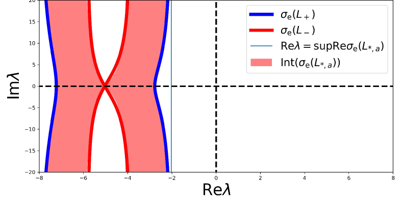
Spectrum of linearized operator, , for a supersonic pulse
7.2 Discrete spectrum for supersonic pulses
In this section we prove that for any , does not have any discrete spectrum to the right of its essential spectrum. That is,
| (7.5) |
proposition 7.2 ensures that if that if (7.1) holds, then which implies spectral stability, along with (7.5).
We now prove (7.5). By definition, if and only if there is an function such that . We rewrite this spectral problem as an equivalent system of ODEs:
| (7.6) |
where is given by (5.3) and is given by (5.4). We show that for all such that , that ; this is the case if for such , all nontrivial solutions of (7.6) are unbounded as . We claim that the matrix has the following properties:
-
(1)
is a mapping into the space of complex square matrices which, for each , varies analytically for all .
-
(2)
exponentially fast as , where is analytic for all .
-
(3)
For all , such that , has two eigenvalues with strictly positive real parts.
Assuming (3) holds, the set of all solutions of ODE are expressible as a linear combinations of (a) either two linearly independent solutions with exponential growth rates equal to the (positive) real parts of eigenvalues of or (b) in the case of a non-diagonal Jordan normal form (due to a degenerate eigenvalue ) a solution with growth and a solution with growth . Hence, all solutions grow exponentially as .
It suffices to verify ()-) for any given , in particular for that satisfies (7.1). Properties ) and ) are trivial. We next show ). Due to the equivalence of the equation to (7.6), the eigenvalues, , of are roots of the characteristic polynomial, arising by seeking solutions of , with ansatz where is a nonzero vector. Recall that , is the weight-conjugated linearized operator evaluated at using the nontrivial equilibrium , where , see (5.8). Therefore, satisfies
These roots are given by
| (7.7) |
Recall that and .
Let
As varies over the set of roots is always equal to . In a neighborhood which is small enough of any point where these roots vary analytically. To be precise, there is a pair of analytic functions and in some small neighborhood of , such that . This is true as long as is not one of the branch points at which , where is the square-root expression appearing in (7.7), where
If is not on the cut of , we can simply choose and , otherwise we just perturb the cut so that is not on it. Therefore, for , is continuous. Note that for , and as . Hence
varies continuously on .
We claim next that for all satisfying , we have that . Indeed, for such that :
| (7.8) |
which implies that for all large , since .
Now consider varying over the region . Suppose is not always positive in this region. Since is continuous, there must be a for which
| (7.9) |
such that . Therefore either or is purely imaginary. Without loss of generality we may assume that for . It follows there is a function , such that . Since , it follows that . However, this contradicts (7.9). This contradiction implies that for all such that (7.9) holds, we have .
Summarizing the result in this section, we have:
Proposition 7.3.
Let denote the linearization about a supersonic pulse, with the weight parameter, , satisfying (7.1). Then,
-
1.
If , then is not in .
-
2.
. In particular, the translation mode: , which satisfies , is not an solution of .
7.3 Remark on instability of subsonic pulses and antikinks
Proposition 6.1 implies, for a TWS to be spectrally stable in some exponential weighted space , it is necessary that both the spectra of asymptotic operators of is in the closed left-half plane. Since we have restricted the weight to be of exponential type defined in (5.1), both of the asymptotic equilibria of need to be spectrally stable in some space, when observed in the reference frame moving with the same speed of . Conversely, if it is impossible to find, WLOG, , such either is stable in , as a result, for any of the exponential type, and is not stable in any with exponential type weight. This is precisely what happens for the subsonic pulses, as well as antikinks.
In fact, since the subsonic pulses and antikinks are all subsonic, it is straightforward to verify that one of the asymptotic equilibria of a subsonic pulse, as well as the equilibrium of an antikink, cannot be rendered spectrally stable in any space since for these equilibria (5.18) is violated.
8 Spectral stability of kinks
Consider a kink profile satisfying (2.13). As noted in remark 6.3, we may restrict our attention to kinks with speed , , where is the solution to (2.13), represented by the solid blue line in figure 5(a). The profile tends to the equilibrium as and to a non-trivial equilibrium at . We have shown in section 5.2.1 that the trivial equilibrium is spectrally stable in the unweighted () space, . We will first characterize the essential spectrum of kinks by applying proposition 6.1 again, before tackling the problem of locating the discrete spectrum.
8.1 Essential spectrum for kinks
Let denote the linearized operator about . Introduce a smooth spatial exponential weight , where
| (8.1) |
The linearized operator whose spectrum determines the spectrum of in is given by ; see (5.5).
Proposition 8.1.
Proof.
The ODE for a kink profile is given in (2.13). The kink is a heteroclinic connection between the trivial equilibrium at and the nontrivial equilibrium at , with ; see Section 2.3.1. By proposition 6.1, the supremum of essential spectrum is determined by the spectra of the asymptotic operators and ; specifically,
The spectrum of is on the imaginary axis, by proposition 5.2, so . Therefore if and only if . By proposition 5.5, the spectrum of is in the closed left-half plane if and only if satisfies (5.17). Hence, if and only if (5.17) is satisfied. Since , condition (5.17) is equivalent to (8.2).
∎
Figure 13 shows a typical case of the essential spectrum of a moving kink.
Spectrum of linearized operator, , for a kink
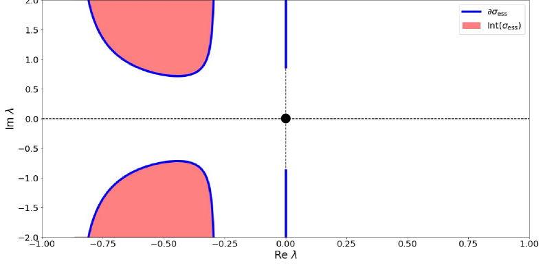
8.2 Neutral spectral stability of Non-moving () kinks
The fact that non-moving kinks are spectrally stable in an appropriate weighted space is a special case of Theorem 8.7 in section 8.3 below. However, the current section 8.2 provides a stronger result and simpler treatment for the special case. Therefore we advise that the readers start with this section first, for pedagogical purposes. In particular, in the current section we do not assume that the nonlinearity satisfies the concavity condition (8.14). Moreover, the transformation (8.10) in the current section is a special case of the one provided in proposition 8.10 in section 8.3, and is less complicated. For non-moving kinks with speed the only possible asymptotic weight as is if it were to be spectrally stable in , as a result of proposition 8.1 where the only possible is . There are four non-moving kinks, each connecting the trivial equilibrium to different nontrivial equilibria, but WLOG we study the one that asymptotes to as , by virtue of Theorem 6.2. The polar angle of this equilibrium on the phase plane of (2.3) is , setting and in (LABEL:eq:_theta_c_E). Now we note that, for this particular kink, in (2.13), which now implies
| (8.3) |
So exponentially as , and exponentially as .
Theorem 8.2 (Neutral spectral stability for non-moving () kinks).
Consider the non-moving kink () namely satisfying (2.13) with , connecting the trivial fixed point and the fixed point on the phase plane. Let such that
Then, is neutrally spectrally stable in , i.e. . In particular,
-
(i)
The essential spectrum of is a subset of the imaginary axis:
where .
-
(ii)
The discrete spectrum of is a subset of gap, on the imaginary axis. Furthermore, always, and is a simple eigenvalue of .
The essential spectrum of a non-moving kink is a subset of the imaginary axis; this is because the spectra of the left- and right-asymptotic operators of , namely and , are all on the imaginary axis. This can be seen from (5.7) and (5.9). In fact:
| (8.4) |
Therefore to prove Theorem 8.2, it suffices to locate the discrete spectrum, since the essential spectrum is the union of and given by (8.4). We consider the eigenvalue problem
| (8.5) |
and and satisfies (8.5). From (5.5) and (5.3) we have an equivalent formulation of (8.5):
| (8.6) |
where
| (8.7) |
Note that for kinks with speed , see (2.13) and set there. Multiplying both sides of (8.6) by the Pauli matrix , we find that (8.6) is equivalent to
| (8.8) |
Introducing an integrating factor, we rewrite (8.8) as
So is a solution of
| (8.9) |
if and only if
| (8.10) |
is a solution to (8.5). That the eigenvalue problem associated with (8.5) is equivalent to the eigenvalue problem associated with equation (8.10), is a consequence of the following lemma, which is proved in appendix C.3:
Lemma 8.3.
Let , and let and be related by (8.10). Then, if and only if .
It then follows immediately that:
Corollary 8.4.
Now, it is convenient to write out (8.9):
| (8.11) | ||||
We are now able to reduce the problem of finding eigenpairs of to finding bound state and bound state energies of some linear Schrödinger operator on the real line, as shown in the following lemma. For proof of this lemma see appendix C.4.
Lemma 8.5.
Assume that the pair where
solves (8.9). Then,
-
(i)
with and , is an eigenpair for the eigenvalue problem:
with the real-valued potential
-
(ii)
Moreover, is the ground state of operator .
We are ready to prove Theorem 8.2
Proof of Theorem 8.2.
It follows from lemma 8.5, by self-adjointness of that and therefore,
| is either real or purely imaginary. |
We may constrain further. Indeed, note that approaches as (since ) and approaches as (since ). Hence, , and . It follows that . It follows that
| is either real or purely imaginary with . | (8.12) |
Now we claim there are no real non-zero eigenvalues of . Once proved, this implies that there are
no eigenvalues with nonzero real part,
and the non-moving kink is neutrally spectrally stable in .
Suppose there exists and that solves (8.5),
then from corollary 8.4 and lemma 8.5
there would be an eigenpair and of the operator .
In fact, this is impossible since is the ground state energy of . Indeed, from (8.11) is a multiple of ,
which does not change sign.
Therefore there is no real eigenvalues of , and proof of Theorem 8.2 is concluded. ∎
Remark 8.6.
We remark that has no embedded eigenvalues in the essential spectrum, see statement (8.12), and that and is a finite subset of the imaginary interval . Indeed, these facts hold for any potential, , satisfying citation of Fadeev criterion
8.3 Spectral stability of moving kinks
Introduce the smooth weight , where
| (8.13) |
We furthermore require the nonlinearity satisfies the following concavity condition:
| (8.14) |
Theorem 8.7.
Assume the nonlinearity satisfies the concavity condition (8.14). Then,
Remark 8.8.
The neutral mode by translation invariance which corresponds to the neutral eigenvalue , is always in the spectrum, since as . In fact, the rate in Theorem 8.7 satisfies
where comes from the decay rate of the kink as , namely (2.19). This is in contrast to the case of supersonic pulses, see proposition 7.3 and the discussion which follows it.
Remark 8.9.
We can improve the result a bit by merely requiring that the parameter in for to satisfy
However for simplicity we made the restriction above. This restriction does not affect our understanding of the “big picture”. Moreover, with this weight, when , the results in Theorem 8.2 are recovered.
Recall for we transformed eigenvalue problem (8.5) to (8.9), through transformation (8.10). We proceed in an analogous manner. We begin with the eigenvalue problem:
| (8.15) |
Explicitly, defined in (5.5) is the (weight-conjugated) linearized operator about a kink of speed :
where and
The expression for is the general expression (5.3) where set set satisfying (2.13) with speed ; the kink profile which tends to as and to as . Here, ; see Section 2.3.1.
Eigenvalue problem (8.15) is rather complicated, in view of the expression of above. However, it is possible to reduce it to a simpler form:
Proposition 8.10.
The proof of proposition 8.10 is given in appendix C.5. Note that setting , transformation (8.10) is recovered from (8.17) and (8.16).
Remark 8.11.
We remark on the intuition behind the transform (C.5) above. Consider the ODE (2.13) which the profiles of kinks and antikinks satisfy (without the restriction on the second line of (2.13)). For , the orbits of possible kinks lie on the -axis, and those of possible antikinks lie on the -axis. In general, however, the kink and lie on the line parallel to vector , and the antikinks and lie on the line parallel to the vector , see figure 5(a); note that for , . We would like to express the perturbation in terms of coordinates along these two vectors, hence the transform (C.5).
The following result states that to preclude unstable discrete spectrum, it suffice to prove that there are no eigenpairs of (8.18).
Lemma 8.12.
We now show there is no that satisfies (8.18) with some . We proceed with shorthand and . Acting on both sides of the second equation of (8.18), then use the first equation for , we obtain a closed equation for
| (8.19) |
Lemma 8.13.
Proof.
Suppose . Then, is also smooth. Take -inner product of with (8.19) and obtain
| (8.20) |
a quadratic equation in . We claim that the coefficients of this quadratic are all non-negative. Note that the quadratic coefficient of (8.20), namely , and
since is monotonically decreasing; so the linear coefficient as well. Furthermore, . In fact, since is monotonically increasing in , and
is monotonically decreasing in . is so by definition, and as a result of the concavity condition (8.14), there is also monotonically decreases in . Therefore and whence . We conclude that is a root of a quadratic polynomial:
where , . It is easily checked that either is one of two negative real roots or its real part is equal to . In all cases, , contradicting the assumption that . As a result there is no with nonnegative real part such that (8.20) holds. This argument carries over for any and we will be done. ∎
Now we summarize the discussion above and give the proof of Theorem 8.7:
Proof of Theorem 8.7.
The essential spectrum of is in the closed left-half plane since , satisfying the condition (8.2) in proposition 8.1.
Assume there was an eigenpair of , where and . Then by lemma 8.12, there would be a pair which would solve the generalized eigenvalue problem (8.18). In particular we would have and . Such would in fact be smooth since the coefficients in (8.18) are bounded and smooth. As a result the pair would solve a generalized eigenvalue problem expressed by a second-order variant coefficient ODE, namely (8.19). However such does not exist by lemma 8.13.
Therefore the assumption does not hold; namely does not have any eigenvalue with a positive real part.
9 Conclusions
There is a large family of heteroclinic traveling wave solutions of (1.1), in both supersonic () and subsonic () regimes; section 2. The bounded heteroclinic traveling waves are either heteroclinic connections between the zero solution and an equilibrium on the unit circle (kinks, antikinks) or heteroclinic connections between distinct equilbria on the unit circle (pulses). For saturable nonlinearities, supersonic pulses are nonlinearly convectively stable against perturbations, which decay rapidly as . This follows from an a priori bound on the growth of general solutions of the IVP and finite propagation speed property for the semilinear hyperbolic system (1.1) (Theorem 4.1). For general nonlinearities, supersonic pulses are linear spectrally stable (Theorem 7.1) in an appropriate weighted space; the spectra of their linearized operators lie in the left half plane. Kinks are linearly and neutrally spectrally stable in suitably weighted spaces: (a) for the case of non-moving kinks (Theorems 8.2) and (b) for arbitrary kinks under a concavity condition on the nonlinearity (Theorem 8.7); section 8; the spectra of their linearized operators lie on the imaginary axis. Antikinks and subsonic pulses are exponentially unstable; section 7.3. Open questions and future directions are discussed in section 1.5.
Appendix A A complete list of the bounded traveling wave solutions
The following list of bounded TWS types is exhaustive.
-
1.
Equilibria. These corresponds to spatially constant time-independent solutions of (1.1):
which are TWSs of arbitrary speeds .
-
2.
Kinks and antikinks. For each , there are four kink-like solutions; in particular, they are , which are kinks, and which are antikinks; for each , there are four kink-like solutions. In particular, they are , which are kinks, and , which are antikinks. See figure 6.
TWSs of all the following types are invariant under .
-
3.
Subsonic pulses. In each of the four following cases there are two subsonic pulse solutions. For each and each they are and ; for each and each they are and ; for each and each they are and ; for each and each they are and .
-
4.
Supersonic pulses. For each of the following cases there are four supersonic pulse solutions, except for the marginal cases which will be indicated. For each and each , these are , which respectively degenerates to at , and and which respectively degenerates to at . For each and each , they are and which respectively degenerates to at , and and which respectively degenerates to at . See figure 3.
-
5.
Periodic wave trains. For each of the following cases there is one periodic wave train solution. In particular, for each and , it is counterclockwise and “small”; for each and each , it is clockwise and “large”; for each and it is clockwise and “small”; for each and each it is counterclockwise and “large”.
Appendix B Proof of proposition 3.1
Recall
| (B.1) |
where is bounded, real-valued and sufficiently smooth,
satisfying , and is the only zero of .
Moreover, there is such that
as , and for each there is such that
as .
Moreover, , the TWS we work with, as well as its components and all their derivatives with respect to ,
asymptotes to their respective limits exponentially as , and are all bounded, in particular we only need to work out the estimate details for terms and in (B.1), since those for and are almost identical.
B.1 Self-mapping properties
B.1.1 Estimates for on
If we have , also ( being weakly differentiable), for each :
Thus
Where only depends on and the profile of .
B.1.2 Estimates for in
The following calculus lemma will be repeatedly used in the sequel.
Lemma B.1.
For positive integers, let Assume
-
(i)
for all , and is bounded.
-
(ii)
There is a nonnegative continuous function on such that
uniformly for all .
Then, there is a constant such that, uniformly in , we have
Proof of lemma B.1.
For any and for all ,
For ,
Hence,
Therefore, uniformly in and for all , we have
∎
B.1.3 Estimates for on
We only need to prove the derivative in of namely the following function is in :
Apply lemma B.1 to to obtain
thus
For a fixed ,
We only need to estimate the expression inside , since is bounded:
the first term can be bounded because decays fast enough as so is bounded since it is also continuous. Then we apply to the second term lemma B.1 and note that is bounded. Therefore
Thus we have:
for a constant depending only on and .
B.2 Lipschitz properties on
B.2.1 is trivially globally Lipschitz
is trivially globally Lipschitz in since it is linear in .
B.2.2 Lipschitz property of
Let . Note that
is bounded:
Integrating both sides we have
Doing the same estimate for and for and we have obtained the global Lipschitz property:
B.3 Lipschitz properties on
B.3.1 is trivially globally Lipschitz on
is trivially globally Lipschitz since it is linear in for and is smooth in .
B.3.2 Lipschitz property of
Now we estimate
the second term can be estimated similarly as in is the Lipschitz estimate above:
To estimate the first term, note that
| (B.2) | ||||
Term is bounded pointwise by
since is bounded. For term , set and define
Then is a bounded function of , and continuously differentiable, vanishes for . Consider the gradient of with respect to for a fixed (suppressing explicit dependence on ):
Both of the terms are bounded uniformly for all . Therefore applying lemma B.1 on , and note that
there is
Where here is a constant only depending on the profile of .
Thus integrating and ,
The last inequality is due to Sobolev embedding.
Appendix C Proofs of some technical results
C.1 Proof of lemma 5.4
If , and and is purely imaginary. Therefore and we are done. Moreover, , for or for . So we can study the case when and .
Consider the conformal mapping from half plane to . Now the line cuts into two path-connected components:
and . Under , transforms to the parabola given by
where . The set is transformed into by , which is the “left” path-connected component of the cut complex plane of which is an element. Now the image of is a subset of the open right-half plane since on is the inverse of . is equivalent to that the image of , , is in ; this is further equivalent to the image of , , is in . In fact,
whose image is
and since , the image of sits to the left (inclusive) of , namely and equivalently , and this is further equivalent to
Now we prove that . In fact, WLOG assume and
which is exactly what needs to be proved.
C.2 Sketch of proof of proposition 6.1
Now the asymptotic operator by (6.2). is constant-coefficient for both and . We can characterize its essential spectrum. We adapt Theorem 3.1.11 and Remark 3.1.14 of Kapitula and Promislow (2013) [KaPr13].
Theorem C.1 (Essential spectrum of ).
if and only if either of the following two statements is true:
-
(i)
-
(ii)
The index of , defined by
(C.1) is not equal to zero.
In the theorem above, is the number of independent vectors such that the following generalized eigenvalue problem is solved with some :
similarly for . The following theorem adapted from the Theorem 3.1.13 of [KaPr13] characterizes the border of :
Theorem C.2 (Characterization of ).
-
(i)
The border of the essential spectrum of is contained in the union of the essential spectra of . Namely
-
(ii)
The set
consists of connected components that are either entirely contained in or does not intersect with it.
We are interested in the essential spectrum of . In fact,
Theorem C.3.
The essential spectra of an and are identical.
Theorem C.3 follows as an immediate corollary of the following Theorem C.4 of Weyl on the invariance of the essential spectrum of a linear operator under relatively compact perturbations [EdEv18], and proposition C.5:
Theorem C.4 (Weyl).
Let be a closed operator between Banach spaces and , and relatively compact to then
We say is relatively compact with respect to , if it is a compact operator on equipped with the graph norm to . For our case, the domain of is , and the graph norm of is equivalent to norm since , with being a invertible constant matrix. To apply Theorem C.4 we need the following proposition
Proposition C.5.
is a relatively compact perturbation of .
Proof.
Note that where
So it can be identified with a piecewise smooth matrix function, with a type-1 discontinuity at . The proof has two steps. First we prove that for any , the operator defined by
is compact relative to . Let be an arbitrary sequence bounded in and as a result of the equivalence of and the graph norm, it is also bounded in the graph norm. Note that
and can be identified with a bounded smooth matrix function on and , respectively. So both sequences are bounded in , therefore both admit convergent subsequences in , as a result of the Rellich-Kondrachev compactness theorem[Hahe2010kolmogorov]; so is their sum . As a result compact from to .
Then we prove is convergent in norm as bounded operators from to . Let be a positive integer and we have
from Sobolev embedding with independent of as long as we fix . Since exponentially fast as , we have
for some independent of , and vanishes as . Thus converges to in operator norm of , the space of bounded linear operators from to . Since is compact in this space, it is compact relative to and the proof is complete. ∎
C.3 Proof of lemma 8.3
It is equivalent to proving that the weight in (8.10) is bounded for all . Equivalently, the exponent
| (C.2) |
is bounded uniformly for . Note that for ; also exponentially as , so exponentially as as well since is bounded for all . As a result, the expression in (C.2) is bounded for all large and negative . For , there is . Also, exponentially fast as , since is also bounded near and exponentially fast as . Thus, for some and all , we have:
for some which is bounded for all . as .
C.4 Proof of lemma 8.5
Written out, (8.9) is
| (C.3) | ||||
It is easy to see in fact is twice continuously differentiable. Now, differentiate the first equation with respect to and using the second to eliminate :
or
where is a time-independent Schrödinger equation with a real-valued potential
Let . We observe that if ; otherwise if and , it would follow from (C.3) that , which contradicts the assumption that .
Now we prove that is an eigenvalue of . From the definition of and in (8.7),
so there is an at which hold that and that its derivative is negative. At , there is
Therefore .
Now is an eigenvalue of . In fact, in this case, and from (C.3) we see since as ,
so cannot be bounded as , unless it vanishes for all , and there is a unique given by (up to a constant):
| (C.4) |
that solves the first of the (now decoupled) equations in (C.3). In fact, direct differentiation yields:
Now for any there is , otherwise, there would be . So has no nodes and thus it is the ground state of , and is the (nondegenerate) ground state energy.
C.5 Proof of proposition 8.10
We will express formulas with Pauli matrices in this proof. See (1.9) and (LABEL:eq:_pauli_commutation). Throughout this proof, .
We must take care when plugging (C.5) into (8.15). Consider a generic differential equation of the form which holds for all . Consequently we have
for all . So write , (8.15) is equivalent to
| (C.6) |
For convenience we further define
| (C.7) |
For satisfying (2.13), since for all and , we have
| (C.8) |
Note that for , satisfies
| (C.9) |
and satisfies
| (C.10) |
Combining (C.9) and (C.10), we see satisfies (C.8) and have value at . Therefore for all ,
and equivalently for all ,
| (C.11) |
Now we transform (8.15) according to (C.6). In the first identity below we used (C.11):
| (C.12) | ||||
In the last line we have used . Using (C.12) above, plug the transformation (C.5) relating with into (C.6), (8.15) is equivalent to
| (C.13) | ||||
In the last identity we have used the fact that and anti-commute for and . See (LABEL:eq:_pauli_commutation). We would like to obtain a differential equation in which there is no coefficient in front of . For this, we multiply on both sides (on the left) by
| (C.14) |
Note that and commute, therefore so does their inverses. Explicitly, we have:
and, note that , there is also
Now multiplying to the left by (C.14) on both sides of the last identity of (C.13):
| (C.15) | ||||
The second term of LHS of (C.15) is
| (C.16) |
the third term:
| (C.17) | ||||
where again . The fourth term is
| (C.18) | ||||
Combining (C.15), (C.16), (C.17) and (C.18):
which is
| (C.19) |
Further, we let
| (C.20) | ||||
which is exactly (8.16). Plugging (C.20) into (C.19) we get rid of the first first term on the RHS of (C.19):
Equivalently, satisfies
| (C.21) |
which is exactly (8.18), and the proof of proposition 8.10 is done.
C.6 Proof of lemma 8.12
By assumption . Since the coefficients of are all bounded and smooth with respect to , is actually smooth. Moreover, with is not in the essential spectrum of since satisfies the condition in proposition 8.1. Hence there are constants with such that as ; similarly for . As a result, if and only if as . From the transform (C.5) relating and , if and only if , if and only if as .
Now assume and rewrite (C.20) as
where
For , , see (C.7); and approaches exponentially fast as . So as . Since , if , there must be (exponentially fast) as .
On the other hand as since for , and exponentially fast. Since (C.21) is also exponentially asymptotically constant, as , also behaves exponentially. There must be where satisfies the following, obtained by taking limits of the coefficients of (C.21) (note that ):
namely . Since as ,
| (C.22) |
This forces since otherwise there must be . Due to the following relation
| (C.23) |
so condition (C.22) is violated. To prove (C.23), note that since , by the following elementary fact:
| (C.24) |
and thus
with , so , and for . As a result (C.23) holds.
So as . Therefore if , there must be exponentially fast as , which implies .
Now we prove inequality (C.24) 444The authors thank Dr. SUN Guanhao of UCSD for pointing out this is not a trivial fact and for providing the following proof.
Proof of (C.24) .
Note that for any ,
| (C.25) |
Write . Since , where . Equation (C.24) becomes . Dividing by , we find that (C.24) is equivalent to
Note that the real part of is always nonnegative, it is equivalent to prove
Using (C.25), the LHS satisfies
with and since the latter requires , contradicting the requirement that . Thus we have concluded the proof of (C.24). ∎