iSLAT: the Interactive Spectral-Line Analysis Tool for JWST and beyond

Abstract

We present iSLAT (the Interactive Spectral-Line Analysis Tool), a python-based graphical tool that allows users to interactively explore and manually fit line emission observed in molecular spectra. iSLAT adopts a simple slab model that simulates emission spectra with a small set of parameters (temperature, emitting area, column density, and line broadening) that users can adjust in real time for multiple molecules or multiple thermal components of a same molecule. A central feature of iSLAT is the possibility to interactively inspect individual lines or line clusters to visualize their properties at high resolution and identify them in the population diagram. iSLAT provides a number of additional features, including the option to identify lines that are not blended at the instrumental resolution, the possibility to save custom line lists selected by the user, and to fit and measure their properties (line flux, width, and centroid) for later analysis. In this paper we launch the tool and demonstrate it on infrared spectra from the James Webb Space Telescope and ground-based instruments that provide higher resolving power. We also share curated line lists that are useful for the analysis of the forest of water emission lines observed from protoplanetary disks. iSLAT is shared with the community on GitHub.

1 Introduction

The analysis of molecular emission spectra in astrophysics can be a daunting challenge due to the overlap of spectral forests of lines, more so if multiple chemical species are present. This is especially true when spectrographs do not have the necessary resolving power to separate individual lines from each other. Famous examples of that are the molecular forests observed at infrared wavelengths with the Spitzer Space Telescope at the resolution of $R\approx 700$ with IRS (Houck et al., 2004), where hundreds of emission blends from H2O, OH, HCN, C2H2, and CO2 were observed from the warm inner regions of protoplanetary disks (Carr & Najita, 2008, 2011; Pontoppidan et al., 2010; Salyk et al., 2011). Even at the $\times 30-100$ higher resolving power provided by ground-based spectrographs, infrared molecular spectra can be dominated by line blending from different molecules and/or emission components (e.g. Najita et al., 2003; Mandell et al., 2012; Brown et al., 2013; Banzatti et al., 2022, 2023a). With the recent and upcoming improvements in resolution and spectral coverage of infrared spectrographs in space and on the ground, the analysis and interpretation of hundreds of emission lines from multiple molecules is at the same time very promising and still very challenging, as demonstrated by the new spectral forests observed with the MIRI spectrograph (Rieke et al., 2015; Wright et al., 2023) on the James Webb Space Telescope (JWST) (e.g. Grant et al., 2023; Gasman et al., 2023; Banzatti et al., 2023b; Pontoppidan et al., 2023).

iSLAT has been built with this potential and challenge in mind, to provide the community with a tool that enables real-time interaction with infrared molecular spectra by comparison to simulated spectra. To handle the combination of large wavelength range and spectral detail of hundreds of lines provided by modern infrared spectrographs, iSLAT features a fully interactive graphical user interface (GUI) that allows users to zoom in/out and pan across the spectra, adjust model parameters for multiple molecules in real time, compare simulated spectra to the data, and perform a number of analysis actions that will be described below.

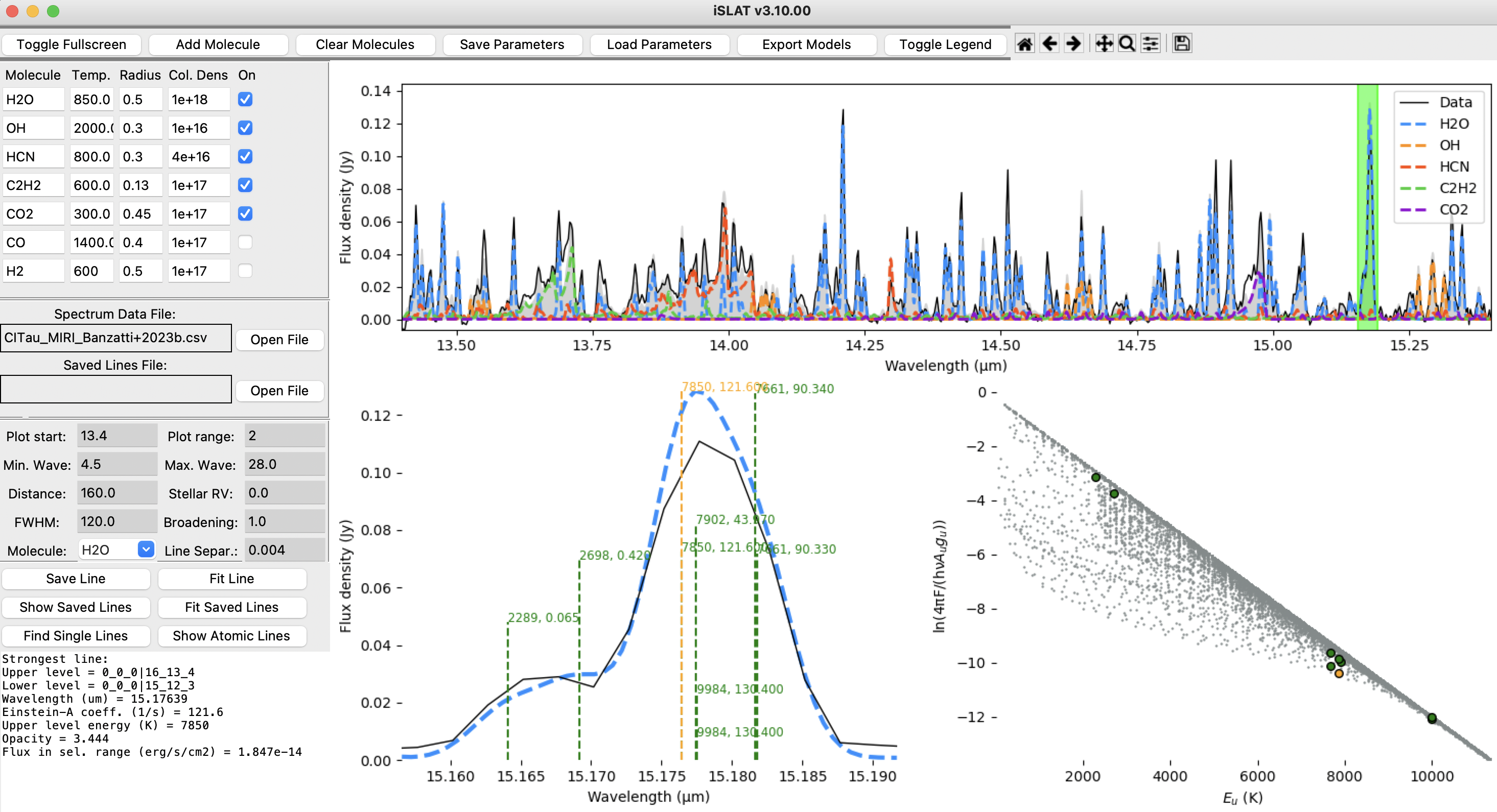
Figure 1: Screenshot of iSLAT’s GUI, using as an example the JWST-MIRI spectrum of CI Tau from Banzatti et al. (2023b). Top graph: observed spectrum (black line) and overlaid model spectra (colored lines). The gray shaded region is the sum of all model spectra selected for plotting. Bottom left graph: Zoomed-in view of the data and H2O model spectrum in the selected wavelength region (light green region in the spectrum graph above). Individual H2O transitions are shown with vertical dashed lines with height proportional to transition intensity for the specific model shown. The strongest line is shown in orange. Bottom right graph: H2O population diagram for the entire model. The specific lines selected in the bottom left are highlighted in the population diagram too. Left: The left side of iSLAT’s GUI provides the user with control over all model parameters and functions. The text box reports action messages and the properties of the strongest line in the selected region.

The slab model code for generating the molecular spectra in iSLAT was written in python by Simon Bruderer and described in the Appendix of Banzatti et al. (2012). The model has four fundamental parameters: the excitation temperature $T$ and the column density $N$ that determine line ratios, the slab surface area $A$ with equivalent emitting radius $R$ that scales all lines equally, and a line width from thermal and turbulent broadening. The synthetic spectra are then scaled to the distance of the specific object, convolved with the instrumental resolution, and shifted to the stellar radial velocity (RV). All these parameters are controlled from the GUI.

iSLAT currently uses line parameters from the HITRAN database and can therefore include any molecule offered with the current HITRAN release (Gordon et al., 2022). A list of six common molecules is loaded into iSLAT by default: CO, H2O, OH, HCN, C2H2, and CO2. Users can then add any other molecules from the HITRAN database as needed in their analyses. Users may also add multiple instances of the same molecule with their own independent parameters. This may be useful, for example, to explore how each parameter affects the molecule spectral excitation in different lines, or when multiple components (or a temperature gradient) of the same molecule are present (e.g. Banzatti et al., 2023a, b; Gasman et al., 2023).

In its conception, iSLAT has been designed to support the analysis of molecular spectra obtained with space telescopes (Spitzer and JWST) and ground-based high-resolution spectrographs (CRIRES, iSHELL, NIRSPEC), with specific reference to the dense forests of lines observed from protoplanetary disks (see e.g. the case of water spectra as observed with multiple instruments in Banzatti et al., 2023a). iSLAT’s flexible structure, however, makes it a versatile tool for molecular spectra observed with other past, present, and future instruments.

2 iSLAT’s GUI and its features

iSLAT’s GUI is illustrated in Figure 1. At the top of the GUI, an interactive matplotlib graph is used to visualize spectra that the user can upload in .csv file format. The input spectrum is assumed to be continuum-subtracted (this needs to be done before using iSLAT) and to have a wavelength (“wave”, in $\mu$m) and flux (“flux”, in Jy) arrays. The input spectrum is plotted on the interactive graph that allows users to pan and zoom on any wavelength region of the spectrum. Within the same graph, iSLAT generates simulated model spectra for multiple molecules that can be overlaid on the data. All model parameters including the temperature (T), column density (N), and equivalent emission radius (R), can be controlled from the GUI for each molecule independently. Any changes in these parameters will adjust the model spectra in the graph in real time. The observed resolution and flux of model spectra is controlled by other parameters in the GUI, including the distance to the observed object and the full width at half maximum (FWHM) of the observed lines, whether that is set by the gas kinematics (if observed at high resolution from the ground) or by the resolving power of the instrument (as in the case of Spitzer and JWST). The model parameters (T, N, R) set by the user for multiple molecules can be saved and loaded for any specific input data spectrum (using the file name as identifier) to allow users to quickly start where they left off at each startup of iSLAT. A text box at the bottom left of the GUI reports messages when specific actions are performed in the GUI (e.g. the temperature of a molecule is updated) and information on any lines selected in the top graph. Additional information from specific functions is printed on terminal, as explained below.

2.1 Spectral-line inspection

Users can select any range in the spectrum graph for inspection at high resolution by clicking and dragging a region (light green region of the top graph in Figure 1). This is one of the central functionalities that motivated the design of iSLAT due to its importance to study molecular spectra as observed at moderate or low resolving powers, as in the case of Spitzer-IRS and JWST-MIRI, where many of the observed emission lines are blend of transitions from multiple energy levels or even from different molecules. After defining a region in the top graph, a zoomed-in version of the data and model spectra in that region will be visualized in the lower-left graph in the GUI. This new graph will visualize the individual transitions as observed at infinite resolution, each one labeled with its upper-level energy and Einstein-$A$ coefficient. The height of transitions visualized in this graph is proportional to the line intensity, with the strongest line in the selected region used as reference. For example, a line that has half the intensity of the strongest line will be half as tall in this graph. Lines that are weaker than 1% of the strongest line are not plotted, to avoid over-crowding the plot.

The properties of the strongest line will be printed in the text box to the left of the graph, including the line upper and lower level quantum numbers, the upper-level energy, the transition wavelength, Einstein-$A$ coefficient, and the opacity at line center (for its definition, see the appendix in Banzatti et al., 2012). A measurement of the line flux is also provided here, as measured by integration of the area below the observed pixels within the region defined by the user. This allows users, for example, to save the flux value for specific regions of interest and use these measurements in their analyses. The properties of the other lines in the selected range are printed on terminal to allow user inspection of weaker lines. The molecule considered in this function is controlled by the drow-down menu in the GUI, i.e. if a user wishes to analyze the spectrum of a molecule other than water (the default), this molecule should be selected in the menu.

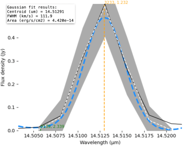
Figure 2: Example of a single line fit using the “Fit Line” function in the GUI. The fit is performed using lmfit and currently adopts a single Gaussian function, which is overlaid as a white dashed line on top of the black data line (the grey area shows the fit uncertainty). The fit results reported in iSLAT’s message box are included in the inset.

The line selected as described above can also be fitted with a Gaussian function using the “Fit Line” button; the fit is done using lmfit and the fit results are added to the message box (Figure 2). The full fit report from lmfit, which includes the uncertainties on model parameters, is printed on terminal for reference. The line centroid from the fit can be used to check for any Doppler shift of the observed lines, for instance due to stellar RV or gas outflows. The line FWHM of individual unresolved lines can be used as a measurement of the instrumental resolving power, e.g. $\sim 110$ km/s in the example shown in Figure 2. This method has been applied to estimate the MIRI resolving power from observed water lines in Pontoppidan et al. (2023).

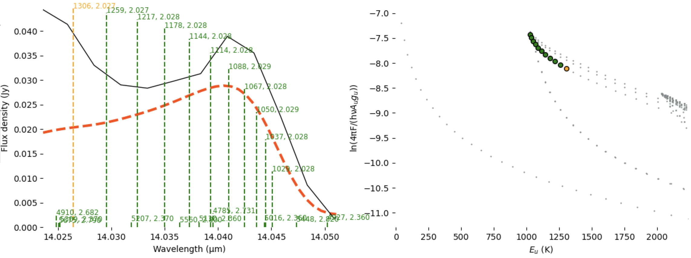
Figure 3: Example of inspection of ro-vibrational lines in the $Q$-branch of HCN. These lines can be blended to water and OH lines, when emission from these molecules is present.

The strongest transition in a chosen spectral region selected as described above can then be appended to a .csv file using the “Save Line” function in the GUI. To use this function, the user has first to select or define an output file under “Saved Lines File”. The line properties will then be appended to the selected .csv file. Any .csv file of previously saved lines can be loaded into iSLAT allowing for the user to identify these lines in the spectrum graph by using the “Show Saved Lines” button. iSLAT’s release includes some line lists that are useful for the analysis of water spectra as observed with JWST-MIRI, see Appendix A.

2.2 Population diagram

In the lower-right part of the GUI, iSLAT includes a plot of the population diagram for a single molecule at a time, as selected from the drop-down menu. The population diagram (also called rotation diagram) is generated in real time for any model parameters set by the user in the GUI, and visualizes the whole spectrum for inspection of excitation conditions and their effects on the population of lines at different upper level energies (for an overview of the technique, see Goldsmith & Langer, 1999). When a user selects a spectral region as described above, all transitions in that region are highlighted in the population diagram too, with the strongest one marked in orange. Figure 3 shows the example of ro-vibrational lines in the $Q$-branch of HCN.

2.3 Identification of isolated lines

iSLAT is built to maximize the prompt and flexible interaction with the data. To this end, the slab models need to run quickly and adjust in real time to user input. The slab model code currently used therefore does not consider the opacity overlap of nearby lines when producing the spectrum. This greatly decreases the computational requirements of the tool and reduces the processing time after adjusting model parameters. However, line opacity overlap has been found to become important for some molecules as observed in protoplanetary disks (Tabone et al., 2023).

To address that, iSLAT includes a filter tool to automatically identify isolated lines that do not overlap. These lines and their associated fluxes can then be used as reference points when fitting a model to the data, while overlapping lines will be overestimated by the model when the column density is high enough for those lines to become partially or fully optically thick. The single-line filter works by first grouping lines in the selected spectral region that are within a given wavelength range from each other (set by the “Line Separation” parameter). Lines that are alone in their group are considered isolated and the filter highlights them in the spectrum graph. For all other groups, the strongest line is identified. The filter then considers the strengths of the other lines in the same group. If the other lines have intensities below a desired percentage (currently set to 10%) of the strongest line in the group, then the strongest line is still considered to be isolated and is highlighted in the spectrum graph. This line selection functionality can be useful for a number of applications besides the line opacity overlap, for instance when users wish to use specific lines or line ratios at different energies as proxies for excitation conditions (e.g. temperature or column density) in modeling explorations.

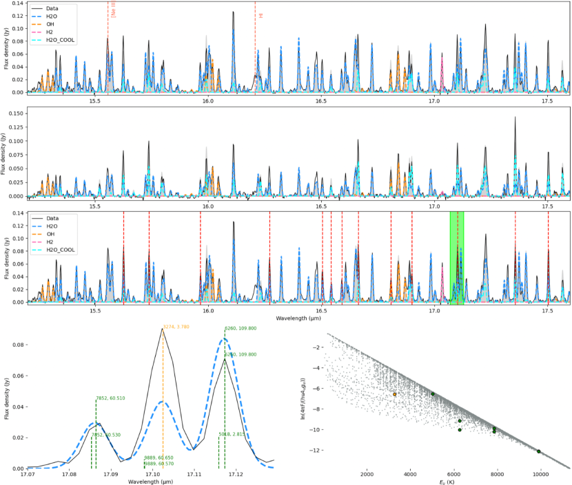
Figure 4: Application of iSLAT to study water temperature components in protoplanetary disks as done in Banzatti et al. (2023b). At the top, the hotter-water dominated case of the large, multi-gapped disk of CI Tau. At the center, the cooler-water dominated case of the compact disk of GK Tau. The two temperatures used for water in this figure are 850 K (in light blue) and 400 K (in cyan, labeled as “H2O cool”). In the third plot, an example of using the “Find Single Lines” function illustrates how even emission lines that look “single” at the resolution of MIRI can be blends of multiple transitions. Only the central line in the selected example is isolated enough to be measured as a single line flux. The model for the hot water emission under-predicts this line, which requires cooler water from a larger emitting area (for more details, see the analysis in Banzatti et al., 2023b).

3 Example Applications

In this section, we present two example applications of iSLAT to analyze molecular spectra observed from space and from the ground.

3.1 Water emission and line blends in MIRI spectra

A first important application of iSLAT is the analysis of the complex spectrum of water as observed with JWST-MIRI. Hundreds of rotational lines are spread across infrared wavelengths, but most of them are close enough to be spectrally blended with lines from other levels when observed at the resolution of MIRI. Figure 4 shows the case of two protoplanetary disks where the water spectrum is dominated by hotter (850 K) vs colder (400 K) water emission, the disks of CI Tau and GK Tau from Banzatti et al. (2023b). With iSLAT, it is easy to compare their spectra to models of water at different temperatures to check which thermal component dominates the observed flux in different emission lines. Blending with other molecules (the case of OH transitions is shown in the figure) can also easily be checked, as well as emission from atomic species that are prominent in some disk spectra (CI Tau in this example).

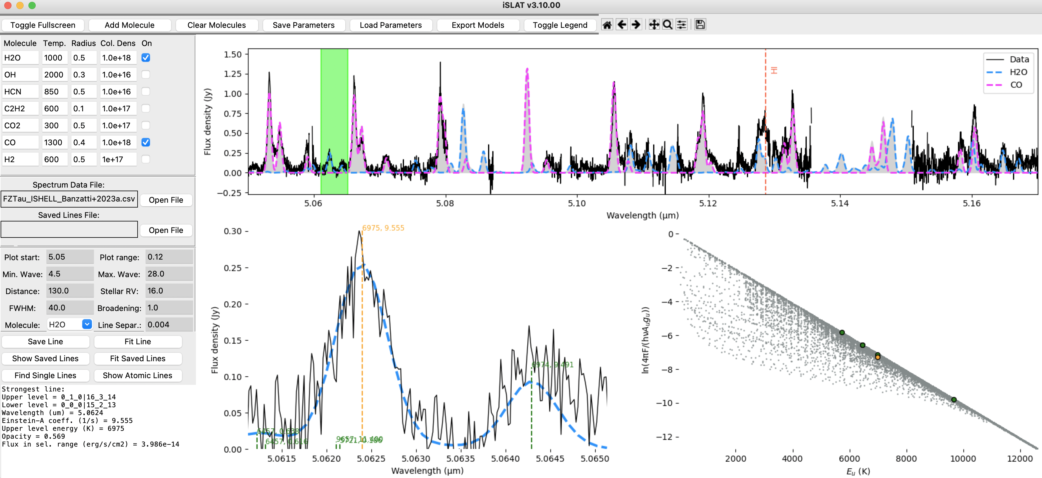
Figure 5: Application of iSLAT to a high-resolution $M$-band spectrum from IRTF-iSHELL for the disk of FZ Tau from Banzatti et al. (2023a). A stellar RV of 16 km/s has been applied to shift the data, as measured from optical spectra (Banzatti et al., 2019). Water lines at these wavelength are predominantly from the fundamental $v=1-0$ band. The gaps in the observed spectrum are due to detector gaps or low telluric transmission.

The bottom of Figure 4 illustrates an example of inspecting water lines for blending from different energy transitions. Using the “Find Single Lines” function, transitions that are not significantly blended with transitions from the same molecule but different energy levels will be marked in the spectrum with a vertical dashed line. Inspection of a complex of three nearby lines shows why only one of them is marked as single: the other two are blends of ortho-para pairs of lines, and in one case include contamination from a lower energy level too. Even at the resolution of MIRI, most of the observed water lines are actually blends of multiple transitions, and iSLAT allows users to identify the single ones in one click. Users may want to explore using different line separation limits (the “Line Separ.” parameter in the GUI) to make sure the line selection is appropriate in different wavelength and resolution conditions. For instance, while a line separation of 0.004 $\mu$m seems to be appropriate for water lines in the 10–27 $\mu$m range of MIRI spectra, a line separation of 0.0011–0.0015 $\mu$m seems more appropriate to identify isolated lines in the ro-vibrational band at 5–8 $\mu$m. Appendix A provides useful lists of isolated water lines relevant for JWST-MIRI spectra and used in recent analyses of protoplanetary disks (Banzatti et al., 2023b). These line lists are also provided to users in the iSLAT GitHub repository, ready to be loaded and visualized in the GUI.

3.2 CO and H2O spectra at high resolving power

Figure 5 shows the application of iSLAT to analyze the CO and H2O emission spectra observed from FZ Tau with the iSHELL spectrograph on IRTF (Rayner et al., 2016, 2022) in Banzatti et al. (2023a). In iSLAT, we can now use the FWHM parameter to match the observed line width as broadened by Keplerian rotation in the disk (in this case, about 40 km/s). The other functions demonstrated above can be used in this case too, to identify atomic lines and inspect line blends. One additional parameter that is essential in the case of high-resolution spectra is the stellar radial velocity (RV) in Heliocentric frame, which will shift the observed spectrum to correct for Doppler shift with the emitting source. In the case of FZ Tau, the RV is about 16 km/s (Banzatti et al., 2019). At these wavelengths water transitions belong to ro-vibrational fundamental bands, predominantly from the first vibrational level down to ground ($v=1-0$) but including some from the second level too ($v=2-1$).

4 Tool release

iSLAT is shared with the community on the GitHub page of the SpExoDisks organization (https://github.com/spexod/iSLAT). A README file guides users through installation and definitions of parameters and functions. A few example spectra from MIRI, iSHELL, and IRS are included in the tool release for users to practice and get familiar with iSLAT; the spectra are continuum subtracted and were originally published in Pontoppidan et al. (2010); Banzatti et al. (2020, 2023a, 2023b); Pontoppidan et al. (2023). The original spectra are available on https://spexodisks.com. We invite the scientific community to contribute to improving and expanding iSLAT on GitHub.

Appendix A Useful line lists for the analysis of water spectra from JWST-MIRI

The tables in this Section report selected water line lists that are useful for the analysis of JWST-MIRI spectra; the full tables are provided to users as .csv files that can be loaded into iSLAT as part of the tool release on GitHub. Water is an asymmetric top molecule with three vibrational ($v_{1}~{}v_{2}~{}v_{3}$, for symmetric stretching, bending, and asymmetric stretching modes respectively) and three rotational ($J~{}K_{a}~{}K_{c}$) quantum numbers, which are included in the table. Transition data are from the current HITRAN release (Gordon et al., 2022).

Table 1 reports single/isolated rotational lines in the ground vibrational level ($v=0-0$) at 10–28 $\mu$m that have been selected using the “Single Lines” function as described in Section 3.1, and additionally filtered to avoid blending with emission from other common molecules.

Table 2 reports ortho-para line pairs in rotational transitions at 10–28 $\mu$m. Most of these transitions are close enough to overlap and contribute to the total opacity of the observed spectral line (see examples in Figure 4).

Table 3 reports rotational lines in the first vibrational level ($v=1-1$) emitting at 10–28 $\mu$m. These lines can be excited enough to be detected in protoplanetary disks, but may show sub-excitation due to non-LTE conditions (Banzatti et al., 2023a). LTE model fits to the spectra may therefore show a discrepancy to the data at these wavelengths, see e.g. the lines at 16.93, 17.31, and 17.68 $\mu$m that are over-predicted by the model in Figure 4.

Table 4 reports single/isolated ro-vibrational lines at 5–8.5 $\mu$m that have been selected using the “Single Lines” function as described in Section 3.1. The ro-vibrational bands at these wavelengths are also usually detected in disks, but typically show sub-excitation due to non-LTE conditions (Bosman et al., 2022; Banzatti et al., 2023a).

Table 1: List of strong isolated (single) H₂O rotational transitions available at JWST-MIRI wavelengths.

Wavelength	Transition (upper-lower levels)	$A_{ul}$	$E_{u}$
($\mu$m)	(level format: $v_{1}v_{2}v_{3}~{}~{}J_{\>K_{a}\>K_{c}}$)	(s-1)	(K)
10.1132	000-000   $17_{\>7\>10}-16_{\>4\>13}$	1.558	6371
10.76435	000-000   $14_{\>9\>6}-13_{\>6\>7}$	0.7628	5302
10.85307	000-000   $15_{\>6\>9}-14_{\>3\>12}$	0.6586	4996
11.00168	000-000   $12_{\>6\>7}-11_{\>1\>10}$	0.06643	3501
11.17771	000-000   $20_{\>8\>13}-19_{\>5\>14}$	14.51	8556
11.2531	000-000   $12_{\>9\>4}-11_{\>6\>5}$	0.2919	4363
11.26877	000-000   $20_{\>7\>14}-19_{\>4\>15}$	16.82	8257
11.61657	000-000   $18_{\>8\>11}-17_{\>5\>12}$	7.511	7244
11.64764	000-000   $17_{\>3\>14}-16_{\>2\>15}$	4.608	5483
11.70161	000-000   $13_{\>5\>8}-12_{\>2\>11}$	0.1994	3783
11.96812	000-000   $14_{\>8\>7}-13_{\>5\>8}$	1.268	4985
12.26544	000-000   $18_{\>7\>12}-17_{\>4\>13}$	12.28	6953
12.5645	000-000   $10_{\>6\>5}-9_{\>1\>8}$	0.03912	2697
12.72945	000-000   $17_{\>7\>11}-16_{\>4\>12}$	9.669	6344
12.89409	000-000   $12_{\>5\>7}-11_{\>2\>10}$	0.2562	3310
12.98575	000-000   $12_{\>7\>5}-11_{\>4\>8}$	0.7422	3759
13.13243	000-000   $16_{\>7\>10}-15_{\>4\>11}$	7.028	5763
13.29319	000-000   $15_{\>3\>12}-14_{\>2\>13}$	3.783	4431
13.50312	000-000   $11_{\>7\>4}-10_{\>4\>7}$	0.4852	3340
13.91485	000-000   $15_{\>5\>11}-14_{\>2\>12}$	6.253	4704
14.19856	000-000   $20_{\>10\>11}-19_{\>9\>10}$	80.31	9218
14.34608	000-000   $14_{\>3\>11}-13_{\>2\>12}$	3.382	3941
14.42757	000-000   $15_{\>4\>11}-14_{\>3\>12}$	6.089	4668
14.51301	000-000   $13_{\>2\>11}-12_{\>1\>12}$	1.232	3232
14.60337	000-000   $19_{\>10\>10}-18_{\>9\>9}$	78.26	8547
14.89513	000-000   $14_{\>5\>10}-13_{\>2\>11}$	5.491	4198
15.62568	000-000   $13_{\>3\>10}-12_{\>2\>11}$	2.988	3474
15.73819	000-000   $12_{\>3\>10}-11_{\>0\>11}$	1.102	2823
15.96622	000-000   $13_{\>5\>9}-12_{\>2\>10}$	4.676	3721
16.27136	000-000   $15_{\>5\>10}-14_{\>4\>11}$	9.232	4835
16.50525	000-000   $17_{\>7\>10}-16_{\>6\>11}$	28.79	6371
16.54402	000-000   $11_{\>6\>6}-10_{\>3\>7}$	1.37	3082
16.59123	000-000   $16_{\>9\>7}-15_{\>8\>8}$	56.44	6369
16.66379	000-000   $12_{\>4\>9}-11_{\>1\>10}$	2.691	3057
16.8082	000-000   $8_{\>6\>2}-7_{\>3\>5}$	0.1388	2031
16.90054	000-000   $9_{\>5\>4}-8_{\>2\>7}$	0.2601	2125
17.10254	000-000   $12_{\>5\>8}-11_{\>2\>9}$	3.78	3273
17.35766	000-000   $11_{\>2\>9}-10_{\>1\>10}$	0.9617	2432
17.50436	000-000   $13_{\>4\>9}-12_{\>3\>10}$	4.941	3645
18.25429	000-000   $11_{\>5\>7}-10_{\>2\>8}$	2.805	2857
18.33865	000-000   $8_{\>4\>4}-7_{\>1\>7}$	0.07159	1628
19.12996	000-000   $15_{\>7\>9}-14_{\>6\>8}$	27.0	5214
19.24597	000-000   $11_{\>3\>8}-10_{\>2\>9}$	2.275	2608
19.34995	000-000   $10_{\>5\>6}-9_{\>2\>7}$	1.829	2472
19.68805	000-000   $14_{\>7\>8}-13_{\>6\>7}$	27.3	4696

Note. — Line properties are from HITRAN (Gordon et al., 2022). The full table is available on GitHub.

Table 2: List of strong H₂O ortho-para line pairs available at JWST-MIRI wavelengths.

Wavelength	Transition (upper-lower levels)	$A_{ul}$	$E_{u}$
($\mu$m)	(level format: $v_{1}v_{2}v_{3}~{}~{}J_{\>K_{a}\>K_{c}}$)	(s-1)	(K)
11.03377	000-000   $17_{\>3\>15}-16_{\>0\>16}$	1.85	5132
11.03475	000-000   $17_{\>2\>15}-16_{\>1\>16}$	1.85	5132
11.72455	000-000   $16_{\>3\>14}-15_{\>0\>15}$	1.682	4620
11.72672	000-000   $16_{\>2\>14}-15_{\>1\>15}$	1.682	4619
13.55068	000-000   $20_{\>12\>8}-19_{\>11\>9}$	118.9	9978
13.55091	000-000   $20_{\>12\>9}-19_{\>11\>8}$	118.9	9978
13.55404	000-000   $19_{\>14\>6}-18_{\>13\>5}$	154.2	10121
13.55404	000-000   $19_{\>14\>5}-18_{\>13\>6}$	154.1	10121
13.73089	000-000   $19_{\>13\>6}-18_{\>12\>7}$	134.3	9708
13.7309	000-000   $19_{\>13\>7}-18_{\>12\>6}$	134.4	9708
13.76219	000-000   $18_{\>16\>2}-17_{\>15\>3}$	190.2	10297
13.76219	000-000   $18_{\>16\>3}-17_{\>15\>2}$	190.2	10297
13.8552	000-000   $18_{\>15\>3}-17_{\>14\>4}$	169.5	9882
13.8552	000-000   $18_{\>15\>4}-17_{\>14\>3}$	169.4	9882
13.95566	000-000   $19_{\>12\>7}-18_{\>11\>8}$	115.1	9305
13.9557	000-000   $19_{\>12\>8}-18_{\>11\>7}$	115.1	9305
13.98964	000-000   $18_{\>14\>4}-17_{\>13\>5}$	149.4	9468
13.98964	000-000   $18_{\>14\>5}-17_{\>13\>4}$	149.4	9468
14.16883	000-000   $18_{\>13\>5}-17_{\>12\>6}$	130.0	9059
14.16883	000-000   $18_{\>13\>6}-17_{\>12\>5}$	130.0	9059
14.21063	000-000   $17_{\>17\>1}-16_{\>16\>0}$	205.7	10062
14.21063	000-000   $17_{\>17\>0}-16_{\>16\>1}$	205.6	10062
14.23737	000-000   $19_{\>11\>8}-18_{\>10\>9}$	96.63	8916
14.2388	000-000   $19_{\>11\>9}-18_{\>10\>8}$	96.57	8916
14.24955	000-000   $17_{\>16\>2}-16_{\>15\>1}$	184.7	9660
14.24955	000-000   $17_{\>16\>1}-16_{\>15\>2}$	184.8	9660
14.33547	000-000   $17_{\>15\>3}-16_{\>14\>2}$	164.4	9252
14.33547	000-000   $17_{\>15\>2}-16_{\>14\>3}$	164.4	9252
14.39851	000-000   $18_{\>12\>6}-17_{\>11\>7}$	111.4	8660
14.39857	000-000   $18_{\>12\>7}-17_{\>11\>6}$	111.4	8660
14.46772	000-000   $17_{\>14\>3}-16_{\>13\>4}$	144.7	8844
14.46772	000-000   $17_{\>14\>4}-16_{\>13\>3}$	144.7	8844
14.64871	000-000   $17_{\>13\>5}-16_{\>12\>4}$	125.8	8440
14.64871	000-000   $17_{\>13\>4}-16_{\>12\>5}$	125.8	8440
14.68765	000-000   $18_{\>11\>7}-17_{\>10\>8}$	93.55	8274
14.68822	000-000   $18_{\>11\>8}-17_{\>10\>7}$	93.53	8274
14.79081	000-000   $16_{\>16\>1}-15_{\>15\>0}$	179.5	9050
14.79081	000-000   $16_{\>16\>0}-15_{\>15\>1}$	179.5	9050
14.86608	000-000   $16_{\>15\>1}-15_{\>14\>2}$	159.5	8650
14.86608	000-000   $16_{\>15\>2}-15_{\>14\>1}$	159.5	8650
14.88384	000-000   $17_{\>12\>6}-16_{\>11\>5}$	107.6	8044
14.88385	000-000   $17_{\>12\>5}-16_{\>11\>6}$	107.6	8044
14.99421	000-000   $16_{\>14\>3}-15_{\>13\>2}$	140.1	8248
14.99421	000-000   $16_{\>14\>2}-15_{\>13\>3}$	140.1	8248

Note. — Line properties are from HITRAN (Gordon et al., 2022). The full table is available on GitHub.

Table 3: List of strong $v=1-1$ H₂O transitions available at JWST-MIRI wavelengths.

Wavelength	Transition (upper-lower levels)	$A_{ul}$	$E_{u}$
($\mu$m)	(level format: $v_{1}v_{2}v_{3}~{}~{}J_{\>K_{a}\>K_{c}}$)	(s-1)	(K)
10.33669	010-010   $17_{\>2\>15}-16_{\>1\>16}$	2.598	7488
10.43161	010-010   $18_{\>4\>15}-17_{\>1\>16}$	6.625	8433
10.9884	010-010   $16_{\>3\>14}-15_{\>0\>15}$	2.322	6974
11.06768	010-010   $18_{\>5\>14}-17_{\>2\>15}$	10.52	8788
11.08288	010-010   $17_{\>3\>14}-16_{\>2\>15}$	5.979	7864
11.45486	010-010   $13_{\>7\>6}-12_{\>4\>9}$	1.107	6681
11.57343	010-010   $18_{\>6\>13}-17_{\>3\>14}$	13.54	9108
11.73657	010-010   $15_{\>3\>13}-14_{\>0\>14}$	2.073	6485
11.74744	010-010   $15_{\>2\>13}-14_{\>1\>14}$	2.07	6484
11.75123	010-010   $16_{\>4\>13}-15_{\>1\>14}$	5.417	7329
11.76071	010-010   $13_{\>6\>7}-12_{\>3\>10}$	1.036	6392
11.81779	010-010   $16_{\>3\>13}-15_{\>2\>14}$	5.376	7322
12.00584	010-010   $17_{\>4\>13}-16_{\>3\>14}$	9.3	8173
12.10458	010-010   $16_{\>7\>10}-15_{\>4\>11}$	6.272	8230
12.28718	010-010   $11_{\>7\>4}-10_{\>4\>7}$	0.4983	5810
12.40411	010-010   $14_{\>7\>8}-13_{\>4\>9}$	2.493	7165
12.44545	010-010   $16_{\>5\>12}-15_{\>2\>13}$	8.52	7640
12.555	010-010   $15_{\>4\>12}-14_{\>1\>13}$	4.864	6814
12.59914	010-010   $14_{\>3\>12}-13_{\>0\>13}$	1.845	6021
12.60313	010-010   $12_{\>7\>6}-11_{\>4\>7}$	0.8958	6228
12.62215	010-010   $14_{\>2\>12}-13_{\>1\>13}$	1.84	6018
12.68409	010-010   $15_{\>3\>12}-14_{\>2\>13}$	4.796	6802
12.75847	010-010   $16_{\>6\>11}-15_{\>3\>12}$	9.816	7930
12.94375	010-010   $16_{\>4\>12}-15_{\>3\>13}$	8.302	7596
13.15066	010-010   $11_{\>6\>5}-10_{\>3\>8}$	0.6687	5515
13.2367	010-010   $11_{\>5\>6}-10_{\>2\>9}$	0.4325	5265
13.2474	010-010   $15_{\>5\>11}-14_{\>2\>12}$	7.513	7105
13.33791	010-010   $15_{\>6\>10}-14_{\>3\>11}$	7.738	7384
13.47704	010-010   $14_{\>4\>11}-13_{\>1\>12}$	4.337	6324
13.4916	010-010   $17_{\>5\>12}-16_{\>4\>13}$	12.73	8395
13.60264	010-010   $13_{\>3\>11}-12_{\>0\>12}$	1.636	5582
13.65169	010-010   $13_{\>2\>11}-12_{\>1\>12}$	1.626	5578
13.72562	010-010   $14_{\>3\>11}-13_{\>2\>12}$	4.239	6305
13.86514	010-010   $14_{\>6\>9}-13_{\>3\>10}$	5.628	6868
14.08938	010-010   $15_{\>4\>11}-14_{\>3\>12}$	7.416	7042
14.1191	010-010   $14_{\>5\>10}-13_{\>2\>11}$	6.465	6597
14.30909	010-010   $13_{\>6\>8}-12_{\>3\>9}$	3.717	6384
14.33815	010-010   $17_{\>12\>5}-16_{\>11\>6}$	120.2	10707
14.45525	010-010   $18_{\>10\>9}-17_{\>9\>8}$	87.23	10493
14.47554	010-010   $9_{\>6\>3}-8_{\>3\>6}$	0.2775	4778
14.53518	010-010   $13_{\>4\>10}-12_{\>1\>11}$	3.829	5861
14.59253	010-010   $17_{\>11\>6}-16_{\>10\>7}$	101.9	10287
14.63497	010-010   $16_{\>13\>4}-15_{\>12\>3}$	134.7	10546
14.65748	010-010   $12_{\>6\>7}-11_{\>3\>8}$	2.228	5932
14.72218	010-010   $16_{\>5\>11}-15_{\>4\>12}$	12.17	7791
14.78088	010-010   $12_{\>3\>10}-11_{\>0\>11}$	1.443	5168

Note. — Line properties are from HITRAN (Gordon et al., 2022). The full table is available on GitHub.

Table 4: List of strong ro-vibrational H₂O transitions available at JWST-MIRI wavelengths.

Wavelength	Transition (upper-lower levels)	$A_{ul}$	$E_{u}$
($\mu$m)	(level format: $v_{1}v_{2}v_{3}~{}~{}J_{\>K_{a}\>K_{c}}$)	(s-1)	(K)
5.2357	010-000   $7_{\>3\>4}-6_{\>2\>5}$	1.27	3543
5.34529	010-000   $10_{\>3\>8}-9_{\>2\>7}$	5.813	4420
5.58362	010-000   $8_{\>2\>7}-7_{\>1\>6}$	7.856	3589
5.61179	010-000   $9_{\>3\>6}-8_{\>4\>5}$	2.009	4179
5.63179	010-000   $7_{\>2\>6}-6_{\>1\>5}$	6.867	3335
5.64107	010-000   $3_{\>3\>0}-2_{\>2\>1}$	5.815	2744
5.70511	010-000   $7_{\>4\>4}-7_{\>3\>5}$	3.115	3696
5.80878	010-000   $8_{\>4\>4}-8_{\>3\>5}$	4.529	3987
5.96224	020-010   $6_{\>0\>6}-5_{\>1\>5}$	20.56	5179
6.0059	020-010   $5_{\>1\>5}-4_{\>0\>4}$	18.77	5010
6.01912	010-000   $6_{\>3\>4}-5_{\>4\>1}$	0.6975	3268
6.07016	010-000   $4_{\>2\>2}-4_{\>1\>3}$	7.676	2766
6.07545	010-000   $3_{\>2\>1}-3_{\>1\>2}$	6.863	2617
6.08018	020-010   $5_{\>1\>4}-5_{\>0\>5}$	6.438	5129
6.14316	010-000   $2_{\>0\>2}-1_{\>1\>1}$	3.778	2395
6.17528	020-010   $2_{\>1\>2}-1_{\>0\>1}$	13.86	4658
6.1854	010-000   $1_{\>1\>0}-1_{\>0\>1}$	10.94	2360
6.19356	030-020   $5_{\>0\>5}-4_{\>1\>4}$	25.99	7188
6.20278	020-010   $3_{\>0\>3}-2_{\>1\>2}$	11.85	4732
6.34443	010-000   $1_{\>0\>1}-1_{\>1\>0}$	12.63	2328
6.37028	010-000   $2_{\>0\>2}-2_{\>1\>1}$	10.99	2395
6.37373	010-000   $2_{\>2\>1}-3_{\>1\>2}$	1.14	2506
6.42663	010-000   $6_{\>4\>3}-7_{\>3\>4}$	0.5998	3450
6.43355	010-000   $5_{\>1\>4}-5_{\>2\>3}$	11.52	2878
6.49224	010-000   $2_{\>1\>2}-3_{\>0\>3}$	7.211	2412
6.52896	010-000   $7_{\>3\>4}-7_{\>4\>3}$	9.451	3543
6.97738	010-000   $9_{\>0\>9}-9_{\>1\>8}$	4.239	3614
6.99328	010-000   $3_{\>2\>2}-4_{\>3\>1}$	8.566	2609
7.14692	010-000   $4_{\>2\>3}-5_{\>3\>2}$	5.629	2745
7.21253	010-000   $7_{\>2\>5}-8_{\>3\>6}$	4.477	3442
7.27924	010-000   $5_{\>3\>2}-6_{\>4\>3}$	8.014	3065
7.30659	010-000   $5_{\>3\>3}-6_{\>4\>2}$	7.835	3059
8.0696	010-000   $10_{\>5\>6}-11_{\>6\>5}$	5.949	4867

Note. — Line properties are from HITRAN (Gordon et al., 2022).

References

- Astropy Collaboration et al. (2022) Astropy Collaboration, Price-Whelan, A. M., Lim, P. L., et al. 2022, ApJ, 935, 167
- Banzatti et al. (2019) Banzatti, A., Pascucci, I., Edwards, S., et al. 2019, ApJ, 870, 76
- Banzatti et al. (2012) Banzatti, A., Meyer, M. R., Bruderer, S., et al. 2012, ApJ, 745, 90
- Banzatti et al. (2020) Banzatti, A., Pascucci, I., Bosman, A. D., et al. 2020, ApJ, 903, 124
- Banzatti et al. (2022) Banzatti, A., Abernathy, K. M., Brittain, S., et al. 2022, AJ, 163, 174
- Banzatti et al. (2023a) Banzatti, A., Pontoppidan, K. M., Pére Chávez, J., et al. 2023a, AJ, 165, 72
- Banzatti et al. (2023b) Banzatti, A., Pontoppidan, K. M., Carr, J. S., et al. 2023b, ApJ, 957, L22
- Bosman et al. (2022) Bosman, A. D., Bergin, E. A., Calahan, J., & Duval, S. E. 2022, ApJ, 930, L26
- Brown et al. (2013) Brown, J. M., Pontoppidan, K. M., van Dishoeck, E. F., et al. 2013, ApJ, 770, 94
- Carr & Najita (2008) Carr, J. S., & Najita, J. R. 2008, Science, 319, 1504
- Carr & Najita (2011) —. 2011, ApJ, 733, 102
- Gasman et al. (2023) Gasman, D., van Dishoeck, E. F., Grant, S. L., et al. 2023, A&A, 679, A117
- Goldsmith & Langer (1999) Goldsmith, P. F., & Langer, W. D. 1999, ApJ, 517, 209
- Gordon et al. (2022) Gordon, I. E., Rothman, L. S., Hargreaves, R. J., et al. 2022, J. Quant. Spec. Radiat. Transf., 277, 107949
- Grant et al. (2023) Grant, S. L., van Dishoeck, E. F., Tabone, B., et al. 2023, ApJ, 947, L6
- Houck et al. (2004) Houck, J. R., Roellig, T. L., van Cleve, J., et al. 2004, ApJS, 154, 18
- Hunter (2007) Hunter, J. D. 2007, Computing in Science and Engineering, 9, 90
- Mandell et al. (2012) Mandell, A. M., Bast, J., van Dishoeck, E. F., et al. 2012, ApJ, 747, 92
- Najita et al. (2003) Najita, J., Carr, J. S., & Mathieu, R. D. 2003, ApJ, 589, 931
- Pontoppidan et al. (2010) Pontoppidan, K. M., Salyk, C., Blake, G. A., et al. 2010, ApJ, 720, 887
- Pontoppidan et al. (2023) Pontoppidan, K. M., Salyk, C., Banzatti, A., et al. 2023, arXiv e-prints, arXiv:2311.17020
- Rayner et al. (2016) Rayner, J., Tokunaga, A., Jaffe, D., et al. 2016, in Society of Photo-Optical Instrumentation Engineers (SPIE) Conference Series, Vol. 9908, Ground-based and Airborne Instrumentation for Astronomy VI, ed. C. J. Evans, L. Simard, & H. Takami, 990884
- Rayner et al. (2022) Rayner, J., Tokunaga, A., Jaffe, D., et al. 2022, Publications of the Astronomical Society of the Pacific, 134, 015002. https://doi.org/10.1088/1538-3873/ac3cb4
- Rieke et al. (2015) Rieke, G. H., Wright, G. S., Böker, T., et al. 2015, PASP, 127, 584
- Salyk et al. (2011) Salyk, C., Pontoppidan, K. M., Blake, G. A., Najita, J. R., & Carr, J. S. 2011, ApJ, 731, 130
- Tabone et al. (2023) Tabone, B., Bettoni, G., van Dishoeck, E. F., et al. 2023, Nature Astronomy, 7, 805
- van der Walt et al. (2011) van der Walt, S., Colbert, S. C., & Varoquaux, G. 2011, Computing in Science and Engineering, 13, 22
- Virtanen et al. (2020) Virtanen, P., Gommers, R., Oliphant, T. E., et al. 2020, Nature Methods, 17, 261
- Wright et al. (2023) Wright, G. S., Rieke, G. H., Glasse, A., et al. 2023, PASP, 135, 048003