Deep Learning for Multivariate Time Series Imputation: A Survey

Abstract

The ubiquitous missing values cause the multivariate time series data to be partially observed, destroying the integrity of time series and hindering the effective time series data analysis. Recently deep learning imputation methods have demonstrated remarkable success in elevating the quality of corrupted time series data, subsequently enhancing performance in downstream tasks. In this paper, we conduct a comprehensive survey on the recently proposed deep learning imputation methods. First, we propose a taxonomy for the reviewed methods, and then provide a structured review of these methods by highlighting their strengths and limitations. We also conduct empirical experiments to study different methods and compare their enhancement for downstream tasks. Finally, the open issues for future research on multivariate time series imputation are pointed out. All code and configurations of this work, including a regularly maintained multivariate time series imputation paper list, can be found in the GitHub repository https://github.com/WenjieDu/Awesome_Imputation.

1 Introduction

The data collection process of multivariate time series in various fields, such as finance Bai and Ng (2008), medicine Esteban et al. (2017), and transportation Gong et al. (2021), is often fraught with difficulties and uncertainty, like sensor failures, instable system environment, privacy concerns, or other reasons. This leads to datasets usually containing a great number of missing values, and can significantly affect the accuracy and reliability of downstream analysis and decision-making. For example, the public real-world medical time series dataset PhysioNet2012 Silva et al. (2012) takes even above 80$\%$ average missing rate, making it challenging to analyze. Consequently, exploring how to reasonably and effectively impute missing components in multivariate time series data is attractive and essential.

The earlier statistical imputation methods have historically been widely used for handling missing data. Those methods substitute the missing values with the statistics (e.g., zero value, mean value, and last observed value Amiri and Jensen (2016)) or simple statistical models, including ARIMA Bartholomew (1971), ARFIMA Hamzaçebi (2008), and SARIMA Hamzaçebi (2008). Furthermore, machine learning techniques like regression, K-nearest neighbor, matrix factorization, etc., have gained prominence in the literature for addressing missing values in multivariate time series. Key implementations of these approaches include KNNI Altman (1992), TIDER Liu et al. (2022), MICE Van Buuren and Groothuis-Oudshoorn (2011), etc. While statistical and machine learning imputation methods are simple and efficient, they fall short in capturing the intricate temporal relationships and complex variation patterns inherent in time series data, resulting in limited performance.

More recently, deep learning imputation methods have shown great modeling ability in missing data imputation. These methods exploit powerful deep learning models like Transformers, Variational AutoEncoders (VAEs), Generative Adversarial Networks (GANs), and diffusion models to capture the intrinsic properties and potentially complex dynamics of time series. In this way, deep learning imputation methods can learn the true underlying data distribution from the observed data, so as to predict more reliable and reasonable values for the missing components. We note that there are several related surveys Khayati et al. (2020); Fang and Wang (2020) that primarily focus on statistical and machine learning imputation methods, but they offer only limited consideration of deep learning imputation methods. Considering that multivariate time series imputation is a crucial data preprocessing step for subsequent time series analysis, a thorough and systematic survey on deep multivariate time series imputation methods would significantly contribute to the advancement of the time series community.

In this paper, we endeavor to bridge the existing knowledge gap by providing a comprehensive summary of the latest developments in deep learning methods for multivariate time series imputation (MTSI). First, we present a succinct introduction to the topic, followed by the proposal of a novel taxonomy, categorizing approaches based on two perspectives: imputation uncertainty and neural network architecture. Imputation uncertainty reflects confidence in imputed values for missing data, and capturing this involves stochastically generating samples and conducting imputations based on these varied samples Little and Rubin (2019). Accordingly, we categorize imputation methods into predictive ones, offering fixed estimates, and generative ones, which provide a distribution of possible values to account for imputation uncertainty. For neural network architecture, we explore a range of deep learning models tailored for MTSI, including Recurrent Neural Network (RNN)-based ones, Graph Neural Network (GNN)-based ones, Convolutional Neural Network (CNN)-based ones, attention-based ones, Variational AutoEncoder (VAE)-based ones, Generative Adversarial Network (GAN)-based ones, and diffusion-based ones. To provide practical imputation guidelines in real scenarios, we conduct extensive empirical studies that examine multiple aspects of deep multivariate time series imputation models, including imputation performance and improvement on downstream tasks like classification. To the best of our knowledge, this is the first comprehensive and systematic review of deep learning algorithms in the realm of MSTI, aiming to stimulate further research in this field. A corresponding resource that has been continuously updated can be found in our GitHub repository.

In summary, the contributions of this paper include: 1) A new taxonomy for deep multivariate time series imputation methods, considering imputation uncertainty and neural network architecture, with a comprehensive methodological review; 2) A thorough empirical evaluation of imputation algorithms via the PyPOTS toolkit we developed; 3) An exploration of future research opportunities for MTSI.

2 Preliminary and Taxonomy

2.1 Background of MTSI

Problem Definition

A complete time series dataset on $[0,T]$ typically can be denoted as $\mathcal{D}=\{\mathbf{X}_{i},\mathbf{t}_{i}\}_{i=1}^{N}$. Hereby, $\mathbf{X}_{i}=\{x_{1:K,1:L}\}\in\mathcal{R}^{K\times L}$ and $\mathbf{t}_{i}=({t_{1},\cdots,t_{L}})\in[0,T]^{L}$, where $K$ is the number of features and $L$ is the length of time series. In the missing data context, each complete time series can be split into an observed and a missing part, i.e., $\mathbf{X}_{i}=\{\mathbf{X}^{o}_{i},\mathbf{X}^{m}_{i}\}$. For encoding the missingness, we also denote an observation matrix as $\mathbf{M}_{i}=\{m_{1:K,1:L}\}$, where $m_{k,l}=0$ if $x_{k,l}$ is missing at timestamp $t_{l}$, otherwise $m_{k,l}=1$. Furthermore, we can also calculate a time-lag matrix $\boldsymbol{\delta}_{i}=\{\delta_{1:K,1:L}\}$ by the following rule,

$$\delta_{k,l}=\left\{\begin{array}[]{ll}{0,}&{\text{if }l=1}\\ {t_{l}-t_{l-1},}&{\text{if }m_{k,l-1}=1\text{ and }l>1}\\ {\delta_{k,l-1}+t_{l}-t_{l-1},}&{\text{if }m_{k,l-1}=0\text{ and }l>1}\end{array}\right.$$

Hence, each incomplete time series is expressed as $\{\mathbf{X}_{i}^{o},\mathbf{M}_{i},\boldsymbol{\delta}_{i}\}$. The objective of MTSI is to construct an imputation model $\mathcal{M}_{\theta}$, parameterized by $\theta$, to accurately estimate missing values in $\mathbf{X}^{o}$. The imputed matrix is defined as:

$$\mathbf{\hat{X}}=\mathbf{{M}}\odot\mathbf{{X}}^{o}+(1-\mathbf{M})\odot\mathbf{\bar{X}},$$ (1)

where $\odot$ denotes element-wise multiplication, and $\mathbf{\bar{X}}=\mathcal{M}_{\theta}(\mathbf{{X}}^{o})$ is the reconstructed matrix. The aim of $\mathcal{M}_{\theta}$ is twofold: (i) to make $\mathbf{\hat{X}}$ approximate the true complete data $\mathbf{X}$ as closely as possible, or (ii) to enhance the downstream task performance using $\mathbf{\hat{X}}$ compared to using the original $\mathbf{X}^{o}$.

Missing Mechanism

The missing mechanisms, i.e., the cause of missing data, represent the statistical relationship between observations and the probability of missing data Nakagawa (2015). In real-life scenarios, missing mechanisms are inherently complex, and the performance of an imputation model is significantly influenced by how closely the assumptions we make align with the actual missing data mechanisms. According to Robin’s theory Rubin (1976), the missing mechanisms fall into three categories: Missing Completely At Random (MCAR), Missing At Random (MAR), and Missing Not At Random (MNAR). MCAR implies that the probability of data being missing is independent of both the observed and missing data. Conversely, MAR indicates that the missing mechanism depends solely on the observed data. MNAR suggests that the missingness is related to the missing data itself and may also be influenced by the observed data. These three mechanisms can be formally defined as follows:

• MCAR: $p(\mathbf{M}|\mathbf{X})=p(\mathbf{M})$,

• MAR: $p(\mathbf{M}|\mathbf{X})=p(\mathbf{M}|\mathbf{X}^{o})$,

• MNAR: $p(\mathbf{M}|\mathbf{X})=p(\mathbf{M}|\mathbf{X}^{o},\mathbf{X}^{m})$.

MCAR and MAR are stronger assumptions compared to MNAR and are considered “ignorable” Little and Rubin (2019). This means that the missing mechanism can be disregarded during imputation, focusing solely on learning the data distribution, i.e., $p(\mathbf{X}^{o})$. In contrast, MNAR, often more reflective of real-life scenarios, is “non-ignorable”, overlooking its missing mechanism can lead to biased parameter estimates. The objective here shifts to learning the joint distribution of the data and its missing mechanism, i.e., $p(\mathbf{X}^{o},\mathbf{M})$.

2.2 Taxonomy of Imputation Methods

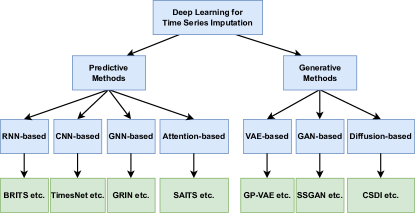
Figure 1: The taxonomy of deep learning methods for multivariate time series imputation from the view of imputation uncertainty and neural network architecture. For each category, one representative model is picked to display.

Method	Venue	Category	Imputation Uncertainty	Neural Network Architecture	Missing Mechanism
GRU-D Che et al. (2018)	Scientific Reports	predictive		RNN	MCAR
M-RNN Yoon et al. (2019)	TBME	predictive		RNN	MCAR
BRITS Cao et al. (2018)	NeurIPS	predictive		RNN	MCAR
TimesNet Wu et al. (2023a)	ICLR	predictive		CNN	MCAR
GRIN Cini et al. (2022)	ICLR	predictive		GNN	MCAR / MAR
SPIN Marisca et al. (2022)	NeurIPS	predictive		GNN, Attention	MCAR / MAR
CDSA Ma et al. (2019)	arXiv	predictive		Attention	MCAR
Transformer Vaswani et al. (2017)	NeurIPS	predictive		Attention	MCAR
SAITS Du et al. (2023)	ESWA	predictive		Attention	MCAR
DeepMVI Bansal et al. (2021)	VLDB	predictive		Attention, CNN	MCAR
NRTSI Shan et al. (2023)	ICASSP	predictive		Attention	MCAR
GP-VAE Fortuin et al. (2020)	AISTATS	generative		VAE, CNN	MCAR / MAR
V-RIN Mulyadi et al. (2021)	Trans. Cybern.	generative		VAE, RNN	MCAR / MAR
supnotMIWAE Kim et al. (2023)	ICML	generative		VAE	MNAR
GRUI-GAN Luo et al. (2018)	NeurIPS	generative		GAN, RNN	MCAR
E2GAN Luo et al. (2019)	IJCAI	generative		GAN, RNN	MCAR
NAOMI Liu et al. (2019)	NeurIPS	generative		GAN, RNN	MCAR
SSGAN Miao et al. (2021)	AAAI	generative		GAN, RNN	MCAR
CSDI Tashiro et al. (2021)	NeurIPS	generative		Diffusion, Attention, CNN	MCAR
SSSD Alcaraz and Strodthoff (2023)	TMLR	generative		Diffusion, Attention	MCAR
CSBI Chen et al. (2023)	ICML	generative		Diffusion, Attention	MCAR
MIDM Wang et al. (2023)	KDD	generative		Diffusion, Attention	MCAR
PriSTI Liu et al. (2023)	ICDE	generative		Diffusion, Attention, GNN, CNN	MCAR
DA-TASWDM Xu et al. (2023)	CIKM	generative		Diffusion, Attention	MCAR
SPD Biloš et al. (2023)	ICML	generative		Diffusion, Attention	MCAR

Table 1: Summary of deep learning methods for multivariate time series imputation.  and  indicate methods capable of accounting for imputation uncertainty, whereas  denotes methods that do not. Furthermore,  denotes that the methods also define the fidelity score to explicitly measure the imputation uncertainty.

To summarize the existing deep multivariate time series imputation methods, we propose a taxonomy from the perspectives of imputation uncertainty and neural network architecture as illustrated in Figure 1, and provide a more detailed summary of these methods in Table 1. For imputation uncertainty, we categorize imputation methods into predictive and generative types, based on their ability to yield varied imputations that reflect the inherent uncertainty in the imputation process. In the context of the neural network architecture, we examine prominent deep learning models specifically designed for time series imputation. The discussed models encompass RNN-based ones, CNN-based ones, GNN-based ones, attention-based ones, VAE-based ones, GAN-based ones, and diffusion-based ones. In the following two sections, we will delve into and discuss the existing deep time series imputation methods from these two perspectives.

3 Predictive Methods

This section delves into predictive imputation methods, and our discussion primarily focuses on four types: RNN-based, CNN-based, GNN-based, and attention-based models.

3.1 Learning Objective

Predictive imputation methods consistently predict deterministic values for the same missing components, thereby not accounting for the uncertainty in the imputed values. Typically, these methods employ a reconstruction-based learning manner with the learning objective being,

$$\mathcal{L}_{det}(\theta)=\sum_{i=1}^{N}\ell_{e}(\mathbf{M}_{i}\odot{\mathbf{\bar{X}}_{i}},\mathbf{M}_{i}\odot\mathbf{X}^{o}_{i}),$$ (2)

where $\ell_{e}$ is an absolute or squared error function.

3.2 RNN-based Models

As a natural way to model sequential data, Recurrent Neural Networks (RNNs) get developed early on the topic of advanced time-series analysis, and imputation is not an exception. GRU-D Che et al. (2018), a variant of GRU, is designed to process time series containing missing values. It is regulated by a temporal decay mechanism, which takes the time-lag matrix $\mathbf{\delta}_{i}$ as input and models the temporal irregularity caused by missing values. Temporal belief memory Kim and Chi (2018), inspired by a biological neural model called the Hodgkin–Huxley model, is proposed to handle missing data by computing a belief of each feature’s last observation with a bidirectional RNN and imputing a missing value based on its according belief. M-RNN Yoon et al. (2019) is an RNN variant that works in a multi-directional way. This model interpolates within data streams with a bidirectional RNN model and imputes across data streams with a fully connected network. BRITS Cao et al. (2018) models incomplete time series with a bidirectional RNN. It takes missing values as variables of the RNN graph and fills in missing data with the hidden states from the RNN. In addition to imputation, BRITS is capable of working on the time series classification task simultaneously. Both M-RNN and BRITS adopt the temporal decay function from GRU-D to capture the informative missingness for performance improvement. Subsequent works, such as Luo et al. (2018, 2019); Liu et al. (2019); Miao et al. (2021), combine RNNs with the GAN structure to output imputation with higher accuracy.

3.3 CNN-based Models

Convolutional Neural Networks (CNNs) represent a foundational deep learning architecture, extensively employed in sophisticated time series analysis. TimesNet Wu et al. (2023a) innovatively incorporates Fast Fourier Transform to restructure 1D time series into a 2D format, facilitating the utilization of CNNs for data processing. Also in GP-VAE Fortuin et al. (2020), CNNs play the role of the backbone in both the encoder and decoder. Furthermore, CNNs serve as pivotal feature extractors within attention-based models like DeepMVI Bansal et al. (2021), as well as in diffusion-based models such as CSDI Tashiro et al. (2021), by mapping input data into an embedding space for subsequent processing.

3.4 GNN-based Models

GNN-based models, treating time series as graph sequences, reconstruct missing values using learned node representations. The authors in Cini et al. (2022) introduce GRIN, the first graph-based recurrent architecture for MTSI. GRIN utilizes a bidirectional graph recurrent neural network to effectively harness both temporal dynamics and spatial similarities, thereby achieving significant improvements in imputation accuracy. Furthermore, SPIN Marisca et al. (2022) is developed, integrating a unique sparse spatiotemporal attention mechanism into the GNN framework. This mechanism notably overcomes the error propagation issue of GRIN and bolsters robustness against the data sparsity presented by highly missing data.

3.5 Attention-based Models

Since Transformer is proposed in Vaswani et al. (2017), the self-attention mechanism has been widely used to model sequence data including time series Wen et al. (2023). CDSA Ma et al. (2019) is proposed to impute geo-tagged spatiotemporal data by learning from time, location, and measurement jointly. DeepMVI Bansal et al. (2021) integrates transformers with convolutional techniques, tailoring key-query designs to effectively address missing value imputation. For each time series, DeepMVI harnesses attention mechanisms to concurrently distill long-term seasonal, granular local, and cross-dimensional embeddings, which are concatenated to predict the final output. NRTSI Shan et al. (2023) directly leverages a Transformer encoder for modeling and takes time series data as a set of timestamp and measurement tuples. As a permutation model, this model has to iterate over the time dimension to process time series. SAITS Du et al. (2023) employs a self-supervised training scheme to deal with missing data, which integrates dual joint learning tasks: a masked imputation task and an observed reconstruction task. This method, featuring two diagonal-masked self-attention blocks and a weighted-combination block, leverages attention weights and missingness indicators to enhance imputation precision. In addition to the above models, the attention mechanism is also widely adapted to build the denoising network in diffusion models like CSDI Tashiro et al. (2021), MIDM Wang et al. (2023), PriSTI Liu et al. (2023), etc.

3.6 Pros and Cons

This subsection synthesizes the strengths and challenges of the predictive imputation methods discussed. RNN-based models, while adept at capturing sequential information, are inherently limited by their sequential processing nature and memory constraints, which may lead to scalability issues with long sequences Khayati et al. (2020). Although CNNs have decades of development and are useful feature extractors to capture neighborhood information and local connectivity, their kernel size and working mechanism intrinsically limit their performance on time series data as the backbone. Due to the attention mechanism, attention-based models generally outperform RNN-based and CNN-based methods in imputation tasks due to their superior ability to handle long-range dependencies and parallel processing capabilities. GNN-based methods provide a deeper understanding of spatio-temporal dynamics, yet they often come with increased computational complexity, posing challenges for large-scale or high-dimensional data.

4 Generative Methods

In this section, we examine generative imputation methods, including three primary types: VAE-based, GAN-based, and diffusion-based models.

4.1 Learning Objective

Generative methods are essentially built upon generative models like VAEs, GANs, and diffusion models. They are characterized by their ability to generate varied outputs for missing observations, enabling the quantification of imputation uncertainty. Typically, these methods learn probability distributions from the observed data and subsequently generate slightly different values aligned with these learned distributions for the missing observation. The primary learning objective of generative methods is thus defined as,

$$\mathcal{L}_{pro}(\theta)=\sum_{i=1}^{N}\log p_{\theta}(\mathbf{{X}}^{o}_{i}).$$ (3)

where $\theta$ is the model parameters of the imputation model $\mathcal{M}$.

4.2 VAE-based Models

VAEs employ an encoder-decoder structure to approximate the true data distribution by maximizing the Evidence Lower Bound (ELBO) on the marginal likelihood. This ELBO enforces a Gaussian-distributed latent space from which the decoder reconstructs diverse data points

The authors in Fortuin et al. (2020) propose the first VAE-based imputation method GP-VAE, where they utilized a Gaussian process prior in the latent space to capture temporal dynamics. Moreover, the ELBO in GP-VAE is only evaluated on the observed features of the data. Authors in Mulyadi et al. (2021) design V-RIN to mitigate the risk of biased estimates in missing value imputation. V-RIN captures uncertainty by accommodating a Gaussian distribution over the model output, specifically interpreting the variance of the reconstructed data from a VAE model as an uncertainty measure. It then models temporal dynamics and seamlessly integrates this uncertainty into the imputed data through an uncertainty-aware GRU. More recently, authors in  Kim et al. (2023) propose supnotMIWAE and introduce an extra classifier, where they extend the ELBO in GP-VAE to model the joint distribution of the observed data, its mask matrix, and its label. In this way, their ELBO effectively models the imputation uncertainty, and the additional classifier encourages the VAE model to produce missing values that are more advantageous for the downstream classification task.

4.3 GAN-based Models

GANs facilitate adversarial training through a minimax game between two components: a generator aiming to mimic the real data distribution, and a discriminator tasked with distinguishing between the generated and real data. This dynamic fosters a progressive refinement of synthetic data that increasingly resembles real samples.

In Luo et al. (2018), authors propose a two-stage GAN imputation method (GRUI-GAN), which is the first GAN-based method for imputing time series data. GRUI-GAN first learns the distribution of the observed multivariate time series data by a standard adversarial training manner, and then optimizes the input noise of the generator to further maximize the similarity of the generated and observed multivariate time series data. However, the second stage in GRUI-GAN needs a lot of time to find the best matched input vector, and this vector is not always the best especially when the initial value of the “noise” is not properly set. Then, an end-to-end GAN imputation model $E^{2}$GAN Luo et al. (2019) is further proposed, where the generator takes a denoising autoencoder module to avoid the “noise” optimization stage in GRUI-GAN. Meanwhile, authors in  Liu et al. (2019) propose a non-autoregressive multi-resolution GAN model (NAOMI), where the generator is assembled by a forward-backward encoder and a multiresolution decoder. The imputed data are recursively generated by the multiresolution decoder in a non-autoregressive manner, which mitigates error accumulation in scenarios involving high-missing and long sequence time series data. On the other hand, in Miao et al. (2021), authors propose USGAN, which generates high-quality imputed data by integrating a discriminator with a temporal reminder matrix. This matrix introduces added complexity to the training of the discriminator and subsequently leads to improvements in the generator’s performance. Furthermore, they extend USGAN to a semi-supervised model SSGAN, by introducing an extra classifier. In this way, SSGAN takes advantage of the label information, so that the generator can estimate the missing values, conditioned on observed components and data labels at the same time.

4.4 Diffusion-based Models

As an emerging and potent category of generative models, diffusion models are adept at capturing complex data distributions by progressively adding and then reversing noise through a Markov chain of diffusion steps. Distinct from VAE, these models utilize a fixed training procedure and operate with high-dimensional latent variables that retain the dimensionality of the input data.

CSDI, introduced in Tashiro et al. (2021), stands out as the pioneering diffusion model specifically designed for MTSI. Different from conventional diffusion models, CSDI adopts a conditioned training approach, where a subset of observed data is utilized as conditional information to facilitate the generation of the remaining segment of observed data. However, the denoising network in CSDI relies on two transformers, exhibiting quadratic complexity concerning the number of variables and the time series length. This design limitation raises concerns about memory constraints, particularly when modeling extensive multivariate time series. In response to this challenge, a subsequent work by Alcaraz and Strodthoff (2023) introduces SSSD, which addresses the quadratic complexity issue by replacing transformers with structured state space models Gu et al. (2022). This modification proves advantageous, especially when handling lengthy multivariate time series, as it mitigates the risk of memory overflow. Another approach CSBI, introduced in  Chen et al. (2023), improves the efficiency by modeling the diffusion process as a Schrodinger bridge problem, which could be transformed into computation-friendly stochastic differential equations.

Moreover, the efficacy of diffusion models is notably influenced by the construction and utilization of conditional information. MIDM Wang et al. (2023) proposes to sample noise from a distribution conditional on observed data’s representations in the denoising process, In this way, it can explicitly preserve the intrinsic correlations between observed and missing data. PriSTI Liu et al. (2023) introduces the spatiotemporal dependencies as conditional information, i.e., provides the denoising network with spatiotemporal attention weights calculated by the conditional feature for spatiotemporal imputation. Additionally, DA-TASWDM Xu et al. (2023) suggests incorporating dynamic temporal relationships, i.e. the varying sampling densities, into the denoising network for medical time series imputation.

Contrasting with the above diffusion-based methods that treat time series as discrete time steps, SPD Biloš et al. (2023) views time series as discrete realizations of an underlying continuous function and generates data for imputation using stochastic process diffusion. In this way, SPD posits the continuous noise process as an inductive bias for the irregular time series, so as to better capture the true generative process, especially with the inherent stochasticity of the data.

4.5 Pros and Cons

This subsection delineates the advantages and limitations of the aforementioned generative imputation models. VAE-based models are adept at modeling probabilities explicitly and offering a theoretical foundation for understanding data distributions. However, they are often constrained by their generative capacity, which can limit their performance in capturing complex data variability. GAN-based models, on the other hand, excel in data generation, providing high-quality imputations with impressive fidelity to the original data distributions. Yet, they are notoriously challenging to train due to issues like vanishing gradients Wu et al. (2023b), which can hamper model stability and convergence. Diffusion-based models emerge as powerful generative tools with a strong capacity for capturing intricate data patterns. Nevertheless, their computational complexity is considerable, and they also suffer from issues related to boundary coherence between missing and observed parts Lugmayr et al. (2022).

5 Time Series Imputation Toolkits

On the time series imputation task, there are existing libraries providing naive processing ways, statistical methods, machine learning imputation algorithms, and deep learning imputation neural networks for convenient usage.

imputeTS Moritz and Bartz-Beielstein , a library in R provides several naive approaches (e.g., mean values, last observation carried forward, etc.) and commonly-used imputation algorithms (e.g., linear interpolation, Kalman smoothing, and weighted moving average) but only for univariate time series. Another well-known R package, mice Van Buuren and Groothuis-Oudshoorn (2011), implements the method called multivariate imputation by chained equations to tackle missingness in data. Although it is not for time series specifically, it is widely used in practice for multivariate time-series imputation, especially in the field of statistics. Impyute and Autoimpute both offer naive imputation methods for cross-sectional data and time-series data. Impyute is only with simple approaches like the moving average window, and Autoimpute integrates parametric methods, for example, polynomial interpolation and spline interpolation. More recently, GluonTS Alexandrov et al. (2020), a generative machine-learning package for time series, provides some naive ways, such as dummy value imputation and casual mean value imputation, to handle missing values. In addition to simple and non-parametric methods, Sktime Löning et al. (2019) implements one more option that allows users to leverage integrated machine learning imputation algorithms to fit and predict missing values in the given data, though this works in a univariate way. When it comes to deep learning imputation, PyPOTS Du (2023) is a toolbox focusing on modeling partially-observed time series end-to-end. It contains more than a dozen deep-learning neural networks for tasks on incomplete time series, including eight imputation models so far.

6 Experimental Evaluation and Discussion

In this section, empirical experiments are conducted to evaluate and analyze deep multivariate time series imputation methods from different categories. The results are obtained with a machine with AMD EPYC 7543 32-Core CPU and an NVIDIA GeForce RTX 4090 GPU. All code, including the data preprocessing scripts, model configurations, and training scripts, are publicly available in the GitHub repository https://github.com/WenjieDu/Awesome_Imputation.

6.1 Datasets and Imputation Methods

Specifically, three naive imputation approaches and eight deep-learning neural networks are tested on three real-world datasets (Air Zhang et al. (2017), PhysioNet2012 Silva et al. (2012), and ETTm1 Zhou et al. (2021) in Table 2) which are commonly used in the literature.

Regarding the imputation methods, apart from three naive ways Mean, Median, and LOCF (last observation carried forward) as baselines, the eight following representative deep-learning models are selected from different categories for experimental studies: M-RNN Yoon et al. (2019), GP-VAE Fortuin et al. (2020), BRITS Cao et al. (2018), USGAN Miao et al. (2021), CSDI Tashiro et al. (2021), TimesNet Wu et al. (2023a), Transformer Du et al. (2023), and SAITS Du et al. (2023). Experiments are performed with PyPOTS Du (2023) and all the above imputation methods are instantly available in the toolbox. Moreover, for a fair comparison, hyperparameters of all deep learning methods are optimized by the tuning functionality in PyPOTS.

	Air	PhysioNet2012	ETTm1
Number of samples	1,458	11,988	722
Sequence length	24	48	96
Number of features	132	37	7
Original missing rate	1.6%	80.0%	0%

Table 2: The general information of the three preprocessed datasets. Note the detailed descriptions are available in the code repository.

Method	Air		PhysioNet2012		ETTm1
	MAE $\downarrow$	MSE $\downarrow$	MAE $\downarrow$	MSE $\downarrow$	MAE $\downarrow$	MSE $\downarrow$
Mean	0.692$\pm$0.000	0.970$\pm$0.000	0.702$\pm$0.000	0.954$\pm$0.000	0.663$\pm$0.000	0.809$\pm$0.000
Median	0.660$\pm$0.000	1.027$\pm$0.000	0.685$\pm$0.000	0.991$\pm$0.000	0.657$\pm$0.000	0.825$\pm$0.000
LOCF	0.206$\pm$0.000	0.279$\pm$0.000	0.411$\pm$0.000	0.569$\pm$0.000	0.135$\pm$0.000	0.072$\pm$0.000
M-RNN	0.524$\pm$0.001	0.648$\pm$0.003	0.674$\pm$0.001	0.864$\pm$0.002	0.651$\pm$0.060	1.074$\pm$0.120
GP-VAE	0.280$\pm$0.003	0.266$\pm$0.009	0.400$\pm$0.007	0.433$\pm$0.011	0.290$\pm$0.017	0.178$\pm$0.015
BRITS	0.142$\pm$0.001	0.129$\pm$0.001	0.246$\pm$0.001	0.325$\pm$0.002	0.124$\pm$0.002	0.046$\pm$0.002
USGAN	0.141$\pm$0.001	0.132$\pm$0.001	0.250$\pm$0.001	0.306$\pm$0.001	0.127$\pm$0.005	0.048$\pm$0.003
CSDI	0.105$\pm$0.003	0.153$\pm$0.021	0.211$\pm$0.003	0.260$\pm$0.050	0.157$\pm$0.052	0.292$\pm$0.456
TimesNet	0.159$\pm$0.002	0.172$\pm$0.003	0.266$\pm$0.007	0.272$\pm$0.006	0.113$\pm$0.006	0.027$\pm$0.002
Transformer	0.163$\pm$0.003	0.160$\pm$0.004	0.209$\pm$0.002	0.225$\pm$0.002	0.133$\pm$0.009	0.035$\pm$0.004
SAITS	0.133$\pm$0.002	0.128$\pm$0.001	0.202$\pm$0.002	0.218$\pm$0.002	0.115$\pm$0.011	0.030$\pm$0.006

Table 3: The MAE and MSE comparisons between imputation methods on the datasets Air,
PhysioNet2012, and ETTm1. The reported values are means $\pm$ standard deviations of five runs.

Method	PR-AUC $\uparrow$	ROC-AUC $\uparrow$
Mean	0.434$\pm$0.016	0.813$\pm$0.009
Median	0.434$\pm$0.018	0.808$\pm$0.014
LOCF	0.425$\pm$0.015	0.804$\pm$0.007
M-RNN	0.424$\pm$0.022	0.807$\pm$0.015
GP-VAE	0.384$\pm$0.018	0.788$\pm$0.008
BRITS	0.428$\pm$0.017	0.821$\pm$0.008
USGAN	0.431$\pm$0.017	0.814$\pm$0.010
CSDI	0.433$\pm$0.017	0.811$\pm$0.005
TimesNet	0.406$\pm$0.012	0.787$\pm$0.013
Transformer	0.446$\pm$0.016	0.807$\pm$0.018
SAITS	0.455$\pm$0.016	0.822$\pm$0.002

Table 4: The means and standard deviations of classification results in five runs.

6.2 Results and Analysis

Imputation Accuracy Evaluation

Imputation results in error metrics MAE (mean absolute error) and MSE (mean squared error) of twelve methods across three datasets are displayed in Table 4. The numbers tell that the performance of the methods varies on different datasets and there is no clear winner in this study. Further work needs to be done to deeply compare predictive and generative imputation methods. Notably, in cases like the Air and ETTm1 datasets, where data is continuously recorded by sensors and the proportion of missingness is relatively low, the non-parametric LOCF method shows commendable performance. Conversely, in the PhysioNet2012 dataset, which has a high missing rate, deep learning imputation methods markedly outperform statistical approaches. This observation corroborates the capability of deep learning methods to effectively capture complex temporal dynamics and accurately learn data distributions, especially in scenarios with highly sparse, discrete observations.

Downstream Task Evaluation

Generally, the better quality of imputed values represents the better overall dataset quality after imputation. Consequently, in addition to the imputation performance comparison, there is an experiment setting in the literature that evaluates the methods from the perspective of downstream task performance Du et al. (2023). Such a study is adopted in this work as well to help assess the selected methods. A simple LSTM model performs the binary classification task on the PhysioNet2012 dataset where each sample has a label indicating whether the patient in the ICU was deceased. The PhysioNet2012 dataset is processed by the imputation methods and the results are presented in Table 4. PR-AUC (area under the precision-recall curve) and ROC-AUC (area under the receiver operating characteristic curve) are chosen to be the metrics, considering the dataset has imbalanced classes and 14.2% positive samples. Note that the only variable in this experiment is the imputed data.

As shown in Table 4, the classifier can benefit from better imputation on the downstream classification task. The best results from SAITS imputation obtain 5% and 1% gains than the best naive imputation Mean separately on the metrics PR-AUC and ROC-AUC. Please note that such improvements are achieved simply by better imputation, which can be seen as a data-preprocessing step in this experiment. Furthermore, this raises a research question about how to make deep learning imputation models learn from both the imputation task and downstream tasks to obtain a consistent and unified representation from the incomplete time series.

Complexity Analysis

We summarize the time and memory complexity of the deep learning imputation models in Table 5. Additionally, their actual inference time on the test set of PhysioNet2012 is also listed for clear comparison.

Method	Computation	Memory	Running Time
M-RNN	$\mathcal{O}(L*K)$	$\mathcal{O}(1)$	5s
GP-VAE	$\mathcal{O}(L*\log{}K)$	$\mathcal{O}(1)$	1s
BRITS	$\mathcal{O}(L)$	$\mathcal{O}(1)$	9s
USGAN	$\mathcal{O}(L)$	$\mathcal{O}(1)$	9s
CSDI	$\mathcal{O}(L^{2})$	$\mathcal{O}(L^{2})$	104s
TimesNet	$\mathcal{O}(L*\log{}K)$	$\mathcal{O}(1)$	1s
Transformer	$\mathcal{O}(L^{2})$	$\mathcal{O}(L^{2})$	1s
SAITS	$\mathcal{O}(L^{2})$	$\mathcal{O}(L^{2})$	1s

Table 5: Computational and space complexity of imputation models, and their running time in seconds on the PhysioNet2012 test set.

7 Conclusion and Future Direction

This paper presents a systematic review of deep learning models specifically tailored for multivariate time series imputation. We introduce a novel taxonomy to categorize the reviewed methods, providing a comprehensive introduction and an experimental comparison of each. To advance this field, the paper concludes by identifying and discussing the following potential avenues for future research.

Missingness Patterns

Existing imputation algorithms predominantly operate under the MCAR or MAR. However, real-world missing data mechanisms are often more complex, with the MNAR data being prevalent in diverse fields such as IoT devices Li et al. (2023), clinical studies Ibrahim et al. (2012), and meteorology Ruiz et al. (2023). The non-ignorable nature of MNAR indicates a distributional shift exists between observed and true data Kyono et al. (2021). For example, in airflow signal analysis Ruiz et al. (2023), the absence of high-value observations causes MNAR missing mechanism and leads to saturated peaks, visibly skewing the observed data distribution compared to the true underlying one. This scenario illustrates how imputation methods may incur inductive bias in model parameter estimation and underperform in the presence of MNAR. Addressing missing data in MNAR contexts, distinct from MCAR and MAR, calls for innovative methodologies to achieve better performance.

Downstream Performance

The primary objective of imputing missing values lies in enhancing downstream data analytics, particularly in scenarios with incomplete information. The prevalent approach is the “impute and predict” two-stage paradigm, where missing value imputation is a part of data preprocessing and followed by task-specific downstream models (e.g. a classifier), either in tandem or sequentially. An alternative method is the “encode and predict” end-to-end paradigm, encoding the incomplete data into a proper representation for multitask learning, including imputation and other tasks (e.g. classification and forecasting, etc.). Despite the optimal paradigm for partially-observed time series data still remains an open area for future investigation, the latter end-to-end way turns out to be more promising especially when information embedded in the missing patterns is helpful to the downstream tasks Miyaguchi et al. (2021).

Scalability

While deep learning imputation algorithms have shown impressive performance, their computational cost often exceeds that of statistical and machine learning based counterparts. In the era of burgeoning digital data, spurred by advancements in communication and IoT devices, we are witnessing an exponential increase in data generation. This surge, accompanied by the prevalence of incomplete datasets, poses significant challenges in training deep models effectively Wu et al. (2023b). Specifically, the high computational demands of existing deep imputation algorithms render them less feasible for large-scale datasets. Consequently, there is a growing need for scalable deep imputation solutions, leveraging parallel and distributed computing techniques, to effectively address the challenges of large-scale missing data.

Large Language Model for MTSI

Large Language Models (LLMs) have catalyzed significant advancements in fields such as computer vision (CV) and natural language processing (NLP), and more recently in time series analysis Jin et al. (2024). LLMs, known for their exceptional generalization abilities, exhibit robust predictive performance, even when confronted with limited datasets. This characteristic is especially valuable in the context of MTSI. LLMs can adeptly mitigate these data gaps by leveraging multimodal knowledge, exemplified by their ability to incorporate additional textual information into analyses Jin et al. (2023), thus generating multimodal embeddings. Such a modeling paradigm not only enriches the imputation process by providing a more holistic understanding and representation of the data but also expands the horizons of MTSI. It enables the inclusion of varied data sources, thereby facilitating a more detailed and context-aware imputation. Exploring the integration of LLMs in MTSI represents a promising direction, with the potential to significantly enhance the efficacy and efficiency of handling missing data in multivariate time series data.

References

- Alcaraz and Strodthoff [2023] Juan Lopez Alcaraz and Nils Strodthoff. Diffusion-based time series imputation and forecasting with structured state space models. Transactions on Machine Learning Research, 2023.
- Alexandrov et al. [2020] Alexander Alexandrov, Konstantinos Benidis, Michael Bohlke-Schneider, Valentin Flunkert, Jan Gasthaus, et al. GluonTS: Probabilistic and Neural Time Series Modeling in Python. Journal of Machine Learning Research, 21(116):1–6, 2020.
- Altman [1992] Naomi S Altman. An introduction to kernel and nearest-neighbor nonparametric regression. The American Statistician, 46(3):175–185, 1992.
- Amiri and Jensen [2016] Mehran Amiri and Richard Jensen. Missing data imputation using fuzzy-rough methods. Neurocomputing, 205(1):152–164, 2016.
- Bai and Ng [2008] Jushan Bai and Serena Ng. Forecasting economic time series using targeted predictors. Journal of Econometrics, 146(2):304–317, 2008.
- Bansal et al. [2021] Parikshit Bansal, Prathamesh Deshpande, and Sunita Sarawagi. Missing value imputation on multidimensional time series. In VLDB, 2021.
- Bartholomew [1971] David J Bartholomew. Time series analysis forecasting and control. Journal of the Operational Research Society, 22(2):199–201, 1971.
- Biloš et al. [2023] Marin Biloš, Kashif Rasul, Anderson Schneider, Yuriy Nevmyvaka, and Stephan Günnemann. Modeling temporal data as continuous functions with stochastic process diffusion. In ICML, 2023.
- Cao et al. [2018] Wei Cao, Dong Wang, Jian Li, Hao Zhou, Lei Li, and Yitan Li. Brits: Bidirectional recurrent imputation for time series. NeurIPS, 2018.
- Che et al. [2018] Zhengping Che, Sanjay Purushotham, Kyunghyun Cho, David Sontag, and Yan Liu. Recurrent neural networks for multivariate time series with missing values. Scientific Reports, 8(1), Apr 2018.
- Chen et al. [2023] Yu Chen, Wei Deng, Shikai Fang, Fengpei Li, Nicole Tianjiao Yang, Yikai Zhang, et al. Provably convergent schrödinger bridge with applications to probabilistic time series imputation. In ICML, 2023.
- Cini et al. [2022] Andrea Cini, Ivan Marisca, and Cesare Alippi. Filling the g_ap_s: Multivariate time series imputation by graph neural networks. In ICLR, 2022.
- Du et al. [2023] Wenjie Du, David Cote, and Yan Liu. SAITS: Self-Attention-based Imputation for Time Series. Expert Systems with Applications, 219:119619, 2023.
- Du [2023] Wenjie Du. PyPOTS: a Python toolbox for data mining on Partially-Observed Time Series. In SIGKDD workshop on Mining and Learning from Time Series, 2023.
- Esteban et al. [2017] Cristóbal Esteban, Stephanie L Hyland, and Gunnar Rätsch. Real-valued (medical) time series generation with recurrent conditional gans. ArXiv Preprint ArXiv:1706.02633, 2017.
- Fang and Wang [2020] Chenguang Fang and Chen Wang. Time series data imputation: A survey on deep learning approaches. arXiv preprint arXiv:2011.11347, 2020.
- Fortuin et al. [2020] Vincent Fortuin, Dmitry Baranchuk, Gunnar Raetsch, and Stephan Mandt. GP-VAE: Deep probabilistic time series imputation. In AISTATS, 2020.
- Gong et al. [2021] Yongshun Gong, Zhibin Li, Jian Zhang, Wei Liu, Yilong Yin, and Yu Zheng. Missing value imputation for multi-view urban statistical data via spatial correlation learning. IEEE Transactions on Knowledge and Data Engineering, 2021.
- Gu et al. [2022] Albert Gu, Karan Goel, and Christopher Re. Efficiently modeling long sequences with structured state spaces. In ICLR, 2022.
- Hamzaçebi [2008] Coşkun Hamzaçebi. Improving artificial neural networks’ performance in seasonal time series forecasting. Information Sciences, 178(23):4550–4559, 2008.
- Ibrahim et al. [2012] Joseph G Ibrahim, Haitao Chu, and Ming-Hui Chen. Missing data in clinical studies: issues and methods. Journal of clinical oncology, 2012.
- Jin et al. [2023] Ming Jin, Qingsong Wen, Yuxuan Liang, Chaoli Zhang, Siqiao Xue, Xue Wang, James Zhang, Yi Wang, Haifeng Chen, Xiaoli Li, et al. Large models for time series and spatio-temporal data: A survey and outlook. arXiv preprint arXiv:2310.10196, 2023.
- Jin et al. [2024] Ming Jin, Shiyu Wang, Lintao Ma, Zhixuan Chu, James Y Zhang, Xiaoming Shi, Pin-Yu Chen, Yuxuan Liang, Yuan-Fang Li, Shirui Pan, and Qingsong Wen. Time-LLM: Time series forecasting by reprogramming large language models. In ICLR, 2024.
- Khayati et al. [2020] Mourad Khayati, Alberto Lerner, Zakhar Tymchenko, and Philippe Cudré-Mauroux. Mind the gap: an experimental evaluation of imputation of missing values techniques in time series. In VLDB, 2020.
- Kim and Chi [2018] Yeo Jin Kim and Min Chi. Temporal Belief Memory: Imputing missing data during rnn training. In IJCAI, 2018.
- Kim et al. [2023] Seunghyun Kim, Hyunsu Kim, Eunggu Yun, Hwangrae Lee, Jaehun Lee, and Juho Lee. Probabilistic imputation for time-series classification with missing data. In ICML, 2023.
- Kyono et al. [2021] Trent Kyono, Yao Zhang, Alexis Bellot, and Mihaela van der Schaar. Miracle: Causally-aware imputation via learning missing data mechanisms. In NeurIPS, 2021.
- Li et al. [2023] Xiao Li, Huan Li, Harry Kai-Ho Chan, Hua Lu, and Christian S Jensen. Data imputation for sparse radio maps in indoor positioning. In ICDE, 2023.
- Little and Rubin [2019] Roderick JA Little and Donald B Rubin. Statistical analysis with missing data, volume 793. John Wiley & Sons, 2019.
- Liu et al. [2019] Yukai Liu, Rose Yu, Stephan Zheng, Eric Zhan, and Yisong Yue. Naomi: Non-autoregressive multiresolution sequence imputation. In NeurIPS, 2019.
- Liu et al. [2022] Shuai Liu, Xiucheng Li, Gao Cong, Yile Chen, and Yue Jiang. Multivariate time-series imputation with disentangled temporal representations. 2022.
- Liu et al. [2023] Mingzhe Liu, Han Huang, Hao Feng, Leilei Sun, Bowen Du, and Yanjie Fu. Pristi: A conditional diffusion framework for spatiotemporal imputation. arXiv preprint arXiv:2302.09746, 2023.
- Löning et al. [2019] Markus Löning, Anthony Bagnall, Sajaysurya Ganesh, Viktor Kazakov, Jason Lines, et al. sktime: A unified interface for machine learning with time series. arXiv preprint arXiv:1909.07872, 2019.
- Lugmayr et al. [2022] Andreas Lugmayr, Martin Danelljan, Andres Romero, Fisher Yu, Radu Timofte, and Luc Van Gool. Repaint: Inpainting using denoising diffusion probabilistic models. In CVPR, 2022.
- Luo et al. [2018] Yonghong Luo, Xiangrui Cai, Ying ZHANG, Jun Xu, and Yuan xiaojie. Multivariate time series imputation with generative adversarial networks. In NeurIPS, 2018.
- Luo et al. [2019] Yonghong Luo, Ying Zhang, Xiangrui Cai, and Xiaojie Yuan. E2GAN: End-to-end generative adversarial network for multivariate time series imputation. In IJCAI, 2019.
- Ma et al. [2019] Jiawei Ma, Zheng Shou, Alireza Zareian, Hassan Mansour, Anthony Vetro, and Shih-Fu Chang. CDSA: cross-dimensional self-attention for multivariate, geo-tagged time series imputation. arXiv preprint arXiv:1905.09904, 2019.
- Marisca et al. [2022] Ivan Marisca, Andrea Cini, and Cesare Alippi. Learning to reconstruct missing data from spatiotemporal graphs with sparse observations. NeurIPS, 2022.
- Miao et al. [2021] Xiaoye Miao, Yangyang Wu, Jun Wang, Yunjun Gao, Xudong Mao, and Jianwei Yin. Generative semi-supervised learning for multivariate time series imputation. In AAAI, 2021.
- Miyaguchi et al. [2021] Kohei Miyaguchi, Takayuki Katsuki, Akira Koseki, and Toshiya Iwamori. Variational inference for discriminative learning with generative modeling of feature incompletion. In ICLR, 2021.
- [41] Steffen Moritz and Thomas Bartz-Beielstein. imputeTS: Time Series Missing Value Imputation in R. The R Journal.
- Mulyadi et al. [2021] Ahmad Wisnu Mulyadi, Eunji Jun, and Heung-Il Suk. Uncertainty-aware variational-recurrent imputation network for clinical time series. IEEE Transactions on Cybernetics, 52(9):9684–9694, 2021.
- Nakagawa [2015] Shinichi Nakagawa. Missing data: mechanisms, methods and messages. pages 81–105. Oxford University Press Oxford, UK, 2015.
- Rubin [1976] Donald B. Rubin. Inference and missing data. Biometrika, 63(3):581–592, 12 1976.
- Ruiz et al. [2023] Joaquin Ruiz, Hau-tieng Wu, and Marcelo A Colominas. Enhancing missing data imputation of non-stationary signals with harmonic decomposition. arXiv preprint arXiv:2309.04630, 2023.
- Shan et al. [2023] Siyuan Shan, Yang Li, and Junier B. Oliva. Nrtsi: Non-recurrent time series imputation. In ICASSP, 2023.
- Silva et al. [2012] Ikaro Silva, George Moody, Daniel J Scott, Leo A Celi, and Roger G Mark. Predicting in-hospital mortality of icu patients: The physionet/computing in cardiology challenge 2012. Computing in cardiology, 39:245, 2012.
- Tashiro et al. [2021] Yusuke Tashiro, Jiaming Song, Yang Song, and Stefano Ermon. CSDI: Conditional score-based diffusion models for probabilistic time series imputation. In NeurIPS, 2021.
- Van Buuren and Groothuis-Oudshoorn [2011] Stef Van Buuren and Karin Groothuis-Oudshoorn. mice: Multivariate imputation by chained equations in r. Journal of statistical software, 45:1–67, 2011.
- Vaswani et al. [2017] Ashish Vaswani, Noam Shazeer, Niki Parmar, Jakob Uszkoreit, Llion Jones, Aidan N Gomez, et al. Attention is all you need. In NeurIPS, 2017.
- Wang et al. [2023] Xu Wang, Hongbo Zhang, Pengkun Wang, Yudong Zhang, Binwu Wang, Zhengyang Zhou, and Yang Wang. An observed value consistent diffusion model for imputing missing values in multivariate time series. In SIGKDD, 2023.
- Wen et al. [2023] Qingsong Wen, Tian Zhou, Chaoli Zhang, Weiqi Chen, Ziqing Ma, Junchi Yan, and Liang Sun. Transformers in time series: A survey. In International Joint Conference on Artificial Intelligence(IJCAI), 2023.
- Wu et al. [2023a] Haixu Wu, Tengge Hu, Yong Liu, Hang Zhou, Jianmin Wang, and Mingsheng Long. TimesNet: Temporal 2D-Variation Modeling for General Time Series Analysis. In ICLR, 2023.
- Wu et al. [2023b] Yangyang Wu, Jun Wang, Xiaoye Miao, Wenjia Wang, and Jianwei Yin. Differentiable and scalable generative adversarial models for data imputation. IEEE Transactions on Knowledge and Data Engineering, 2023.
- Xu et al. [2023] Jingwen Xu, Fei Lyu, and Pong C Yuen. Density-aware temporal attentive step-wise diffusion model for medical time series imputation. In CIKM, 2023.
- Yoon et al. [2019] Jinsung Yoon, William R. Zame, and Mihaela van der Schaar. Estimating missing data in temporal data streams using multi-directional recurrent neural networks. IEEE Trans. on Biomedical Engineering, 2019.
- Zhang et al. [2017] Shuyi Zhang, Bin Guo, Anlan Dong, Jing He, Ziping Xu, and S. Chen. Cautionary tales on air-quality improvement in beijing. Proceedings of the Royal Society A: Mathematical, Physical and Engineering Sciences, 473, 2017.
- Zhou et al. [2021] Haoyi Zhou, Shanghang Zhang, Jieqi Peng, Shuai Zhang, Jianxin Li, Hui Xiong, and Wancai Zhang. Informer: Beyond efficient transformer for long sequence time-series forecasting. In AAAI, 2021.