Abstract

Global Climate Models (GCM) are very useful tools to study theoretically the general dynamics and specific phenomena in planetary atmospheres. In the case of Venus, several GCMs succeeded in reproducing the atmosphere’s superrotation and the global temperature field. However, the highly variable polar temperature and the permanent cold collar present at $60\degree-80\degree$ latitude have not been reproduced satisfactorily yet.

Here we improve the radiative transfer scheme of the Institut Pierre Simon Laplace Venus GCM in order to numerically simulate the polar thermal features in Venus atmosphere. The main difference with the previous model is that we now take into account the latitudinal variation of the cloud structure. Both solar heating rates and infrared cooling rates have been modified to consider the cloud top’s altitude decrease toward the poles and the variation in latitude of the different particle modes’ abundances.

A new structure that closely resembles the observed cold collar appears in the average temperature field at $2\times 10^{4}-4\times 10^{3}$ Pa ($\sim 62-66$ km) altitude range and $60\degree-90\degree$ latitude band. It is not isolated from the pole as in the observation-based maps, but the obtained temperature values (220 K) are in good agreement with observed values. Temperature polar maps across this region show an inner warm region where the polar vortex is observed, but the obtained 230 K average value is colder than the observed mean value and the simulated horizontal structure does not show the fine-scale features present within the vortex.

The comparison with a simulation that does not take into account the latitudinal variation of the cloud structure in the infrared cooling computation, shows that the cloud structure is essential in the cold collar formation. Although our analysis focuses on the improvement of the radiative forcing and the variations it causes in the thermal structure, polar dynamics is definitely affected by this modified environment and a noteworthy upwelling motion is found in the cold collar area.

Kew words: Venus atmosphere, cold collar, modelling.

1 Introduction

In the last two decades, Global Climate Models (GCMs) have turned out to be very useful tools to study the general atmospheric circulation on Venus and the role of different phenomena in the angular momentum budget. Several numerical simulations by different GCMs have already reproduced the main characteristic of the Venus atmosphere: its superrotation (e.g. Yamamoto and Takahashi,, 2003; Lee et al.,, 2007; Sugimoto et al., 2014a, ; Lebonnois et al.,, 2016). At about 70 km altitude clouds circle the solid planet at $\sim$100 m/s, sixty times faster than the rotation of the planet. These simulations support the Gierasch-Rossow-Williams mechanism (Gierasch,, 1975; Rossow and Williams,, 1979) to explain the maintenance of the superrotation, which holds the latitudinal transport of angular momentum by horizontal planetary-scale waves and by the meridional circulation responsible for the velocity field in the atmosphere. GCMs also confirmed that in the case of Venus, the thermal tides play a key role in transporting the angular momentum vertically (Takagi and Matsuda,, 2007; Lebonnois et al.,, 2010). On the other hand, it is well known that there is a wide variety of waves in the main cloud deck (Belton et al.,, 1976; Rossow et al.,, 1980; Del Genio and Rossow,, 1990; Peralta et al.,, 2008; Piccialli et al.,, 2014) that may contribute to the transport of angular momentum and, therefore, recent GCMs studies have focused on the analysis of the wave activity present in the Venusian atmosphere (Sugimoto et al., 2014b, ; Lebonnois et al.,, 2016).

One of the pending questions for the Venus GCMs is the simulation of the atmospheric thermal structure. Although the average temperature field has been reproduced adequately, no model has satisfactorily simulated one of its most puzzling properties: the polar temperature distribution, formed by highly variable vortices and cold air areas that surround the vortices permanently (Zasova et al.,, 2007; Tellmann et al.,, 2009).

The temperature in the deep atmosphere is almost constant from equator to around $50\degree$, and slowly decreases polewards (Tellmann et al.,, 2009). However, above $\sim$70 km altitude temperatures increase from equator to pole, in contrast to what is expected from radiative-convective equilibrium, since solar heating is higher at equator than at the poles. This is known as the warm polar mesosphere. At 60 - 70 km altitude the temperature field in the $60\degree-80\degree$ region has a striking feature in both hemispheres, a strong temperature inversion called the cold collar (Taylor et al.,, 1980). It is a collar of cold air circling each pole of Venus. The latitudinally averaged temperature between $60\degree$ and $80\degree$ is about 20 K colder than at the equator and 15 K colder than at the poles, i.e. between $80\degree$ and $90\degree$ (Haus et al.,, 2014). This temperature difference would cause it to dissipate rapidly, however the cold collar is a permanent structure at the sub-polar latitudes of Venus, implying that it is forced by some unknown mechanism. Enclosed by the cold collar there is a warm polar vortex in each pole of Venus. These are rapidly rotating cloud and temperature structures that show highly variable and complex morphologies with warm small-scale filaments (Piccioni et al.,, 2007; Luz et al.,, 2011; Garate-Lopez et al.,, 2013). This region features the greatest horizontal temperature gradient at the cloud top level. Neither the cold collar nor the warm vortex are completely uniform along the latitude circles (Grassi et al.,, 2010; Garate-Lopez et al.,, 2015); therefore, the latitudinally averaged temperature field hides the real thermal contrast between these two features. The mean temperature difference between the coldest area of the cold collar and the warmest nucleus of the vortex is $\sim$30 K, but the temperature gradient can be as high as $dT/dr$ = 0.1 K/km ($\delta T$ = 50 K over 500 km) in this region (Garate-Lopez et al.,, 2015).

Although these polar structures have been observed repeatedly, their origin and formation mechanism are still unknown and, therefore, numerical studies of the Venusian polar region were recently conducted (Yamamoto and Takahashi,, 2015; Ando et al.,, 2016, 2017; Lebonnois et al.,, 2016). Using GCMs that force the temperature structure with Newtonian cooling and previously prepared heating rate profiles, Yamamoto and Takahashi, (2015) and Ando et al., (2016) concluded that thermal tides play an important dynamical role in the formation of the cold collar and warm vortex. The former stated that the baroclinic waves are also part of the formation mechanism while the latter attributed the origin of the polar structures to the combination of the thermal tides and the residual meridional circulation. Ando et al., (2017) investigated the vertical structure of the temperature fluctuation in the Venusian polar atmosphere by comparing radio occultation measurements and GCM results, and concluded that the thermal disturbance associated to the polar vortex could be a neutral barotropic Rossby wave related to barotropic instability. These three works obtained a temporally evolving polar region and some horizontal structure within the vortex. However, the average latitude-altitude distributions of temperature do not exactly reproduce the observed cold collar structure. In observation-based maps (Zasova et al.,, 2007; Tellmann et al.,, 2009; Haus et al.,, 2014) the cold collar is an isolated region and is located slightly lower than in the maps of Yamamoto and Takahashi, (2015) and Ando et al., (2016, 2017). In addition, the average temperature values obtained by Ando et al., (2016) are not warm enough compared to observations.

On the other hand, Lebonnois et al., (2016) used the IPSL (Institut Pierre Simon Laplace) Venus GCM, that has a full radiative transfer module, to model the Venus atmosphere paying a special attention to polar regions. Their zonally and temporally averaged latitudinal profiles showed a small cold collar signature at the cloud top ($\sim$70 km), located slightly higher than observed. Due to its axi-asymmetric distribution, the obtained cold collar looked subtle when zonally averaged but it was more evident in the polar temperature fields. They related the shape of the polar temperature distribution (cold collar and warm vortex) to the combination of thermal tide and high-frequency wave activity but the temperature contrasts obtained inside the polar regions ($\sim$10 K) were weaker than those presented by Ando et al., (2016, 2017) ($\sim$20-25 K) and were far from the observed $\sim$30 K on average (Garate-Lopez et al.,, 2015).

In order to perform an in-depth study of the Venus polar atmosphere and try to better understand the origin and nature of the cold collar and warm vortex, we have adapted the IPSL Venus GCM by taking into account the latitudinal variation of the cloud structure (not considered in any GCM mentioned above). The details about the improvements on the radiative transfer scheme are described in Section 2. Then, Section 3 shows the average temperature and zonal wind fields obtained by the current model, which are in better agreement with observations and reproduce the characteristic cold collar feature in a more realistic way than previously. We discuss the formation of the cold collar in terms of radiative transfer effects in Section 4 and we sum up the conclusions in Section 5.

2 Simulations

2.1 IPSL Venus GCM

The general characteristics of the IPSL Venus GCM have been described in detail in Lebonnois et al., (2010) and Lebonnois et al., (2016). Therefore, only a short summary is given here. The model is based on the LMDZ latitude-longitude grid finite-difference dynamical core (Hourdin et al.,, 2006). Since the goal of the current study is the polar regions, it must be noted that this dynamical core includes a longitudinal polar filter that limits the effective resolution to that at mid-latitudes. Some of the most important features of the model are: the boundary layer scheme used, based on Mellor and Yamada, (1982); the implementation of topography, with hybrid vertical coordinates (50 vertical levels, from surface to roughly 95 km altitude); the temperature dependence of the specific heat $C_{p}(T)$, which affects the definition of the potential temperature (as detailed in Lebonnois et al.,, 2010); and the horizontal resolution currently used, 96 longitudes x 96 latitudes, i.e. 3.75° x 1.875°.

The previous version of the model (Lebonnois et al.,, 2016) reproduced consistently the average zonal wind and temperature fields, but the obtained equatorial jet was too intense compared to mid-latitude jets and the winds below the clouds were too slow compared to measurements made by Venera and Pioneer Venus probes (Schubert,, 1983; Gierasch et al.,, 1997). On the other hand, the modeled average temperature structure, although generally consistent with observations, resulted in colder temperatures in the deep atmosphere and at surface compared to observed profiles (Seiff et al.,, 1985), and in slightly higher temperatures above the clouds (Tellmann et al.,, 2009; Migliorini et al.,, 2012; Grassi et al.,, 2014). The latitudinal profiles showed a small cold collar signature at $\sim$70 km and the polar temperature distribution at $\sim$67 km displayed some inner structure. However, in the average altitude-latitude temperature map the cold collar was not an isolated feature as in observation-based maps (Tellmann et al.,, 2009; Haus et al.,, 2014) and the contrast between cold collar and warm vortex was weaker than observed, about 10 K in the model vs $\sim$30 K in temperature retrievals from VIRTIS instrument (Garate-Lopez et al.,, 2015). The latitudinal structure of the clouds was not taken into account in this previous IPSL model, though Lebonnois et al., (2016) noted that it could play a role in the shape and strength of the cold collar.

Due to the development of different tools necessary to implement the latitudinal variation of the cloud structure in the solar heating rates and in the infrared cooling rates, the improvements in the radiative transfer were done in two stages; (1) implementation of the cloud structure in the solar heating rates, plus some tuning, and (2) implementation of the cloud structure in the IR cooling rates (these improvements and tuning are described in the next section). The simulation started from an already superrotating atmosphere obtained from previous simulations (Lebonnois et al.,, 2016) and it was then run for 200 Venus days (Vd, 117 Earth days) with the partially-improved radiative transfer, the one obtained after the first stage of the improvements. Two simulations were then pursued for another 100 Vd: one with latitudinally uniform clouds in the IR cooling computation (referred to as unifcld hereon) and another one with latitudinal variations of the cloud structure for studying the cold collar (varcld hereon). The former case, unifcld simulation, is used for control by comparing it to the varcld simulation in the discussion of the formation of the cold collar, but this simulation and its results have no physical sense and should not be considered alone. In the latter case (varcld simulation) a stable state of the atmosphere was obtained after roughly 60 Vd of simulation, so it is the simulation that represents the current IPSL Venus GCM model. The different inputs used in each stage and simulations are summarized in Table 1.

TABLE 1

2.2 Improved radiative transfer

Previously, the radiative transfer included solar heating rate profiles as a function of solar zenith angle taken from look-up tables based on Crisp, (1986), and used the infrared net-exchange rate matrix formulation (Eymet et al.,, 2009) with horizontally uniform opacity sources (gas and clouds).

For the current study, the main modification in the radiative transfer is related to the cloud model. Our computations now take into account the more recent cloud model described by Haus et al., (2014, 2015), which is based on the most recent observations performed by the Venus-Express spacecraft. In particular, this model describes latitudinal variations of the cloud structure. According to Haus et al., (2014), the cloud top altitude (defined as the altitude where the optical depth equals the unity at 1 $\mu$m) decreases slowly from about 71 km at the equator to about 70 km at $50\degree$, but then it quickly drops poleward reaching about 61 km over both poles. Authors also found a strong latitude dependence of cloud opacity, which is transposed into the latitudinal behavior of cloud mode factors, scaling the abundance of the different modes compared to the equatorial vertical distribution. Retrieved mode 1 and 2 factors gradually decrease poleward of $30\degree$ showing a small local minimum at $55\degree$. The mode 3 factor is nearly constant from equator to $\sim 15\degree$, decreases between $15\degree$ and $30\degree$, remains almost constant up to $55\degree$, but then strongly increases poleward (Haus et al.,, 2014). This new cloud model and some tuning (see details below) were implemented both in the solar heating and infrared cooling rates’ computations.

2.2.1 Solar heating

For the short-wavelength part of the radiative transfer scheme, the principle used is basically the same as previously. Look-up tables are used, that contain the vertical profile of the solar heating rate as a function of solar zenith angle. The model described in Haus et al., (2015) is now used to produce these tables. In addition, since the latitudinal structure of the cloud is now taken into account, the tables vary with latitude, in bins of $5\degree$. It can be noted that in this cloud model, the unknown ultraviolet absorber is modeled independently from the cloud particle modes, regardless of the absorber’s chemical composition.

The vertical profile of the solar heating plays a crucial role in the temperature profile, as shown e.g. by Lebonnois et al., (2015). However, it is poorly constrained by available data. A series of tests were performed with the new solar heating rates (Lebonnois and Schubert,, 2017, Methods and Supplementary Materials). Below approximately the cloud base, these solar heating rates are smaller than the ones that were used previously (Crisp,, 1986), and this resulted in deep atmospheric temperature profiles significantly colder than observed. The composition of the lower haze particles, located between the cloud base (48 km) and 30 km and observed by in-situ probe instruments (Knollenberg et al.,, 1980), is not established, so their optical properties are not well constrained. This sub-cloud haze is not taken into account in the Haus et al., (2015) model, except for the tail of the sulfuric acid cloud mode vertical distributions. The absorption of the solar flux in this region is therefore subject to uncertainty. To better reproduce the temperature structure in the middle cloud and below, we decided to increase the solar heating rates in this region, multiplying the solar heating rates provided by the Haus et al., (2015) model by a factor of 3. This tuning brings the values in the same range as other models (Crisp,, 1986; Lee and Richardson,, 2011), and allows the temperature profile to reach observed values.

2.2.2 Infrared cooling

The long-wavelength part of the radiative transfer scheme is based on the net-exchange rate (NER) formalism (Eymet et al.,, 2009). The cloud model (density profile of each mode, $n_{i}(z)$) used in the previous computation of the net-exchange rate matrices was from Zasova et al., (2007). In this work, we now use the cloud model described in Haus et al., (2014). In order to take into account the latitudinal variations of this model, matrices are computed for five latitudinal bins: $0\degree$ - $50\degree$, $50\degree$ - $60\degree$, $60\degree$ - $70\degree$, $70\degree$ - $80\degree$ and $80\degree$ - $90\degree$. When running the GCM, the matrices are interpolated between the central latitudes of each bin.

The gas opacities are computed first for high-resolution spectra, taking into account updated spectral dataset, Voigt line shape profiles, and a truncation at 200 cm^-1. Then correlated-k coefficients are computed and used in the NER matrix calculation. In addition, CO₂ and H₂O collision-induced absorption are taken into account, as detailed in Lebonnois et al., (2015). However, as mentioned in Lebonnois et al., (2015) and Lebonnois and Schubert, (2017), it is difficult to have consistent temperature profiles in the middle and lower cloud and in the atmosphere below without including some small additional continuum to close the windows located in the [3 - 7] $\mu$m range, through which energy is exchanged between the cloud base and the layers just below. Here, an additional continuum of $1.3\times 10^{-6}$cm^-1amagat^-2 is taken into account in the 30 - 48 km region, and $4\times 10^{-7}$cm^-1amagat^-2 in the 16 - 30 km region, for a best fit of the VIRA (Seiff et al.,, 1985) and VeGa-2 (Linkin et al.,, 1987; Zasova et al.,, 2006) temperature profiles (see Lebonnois and Schubert,, 2017, Methods and Supplementary Information).

3 Results

3.1 Average temperature field

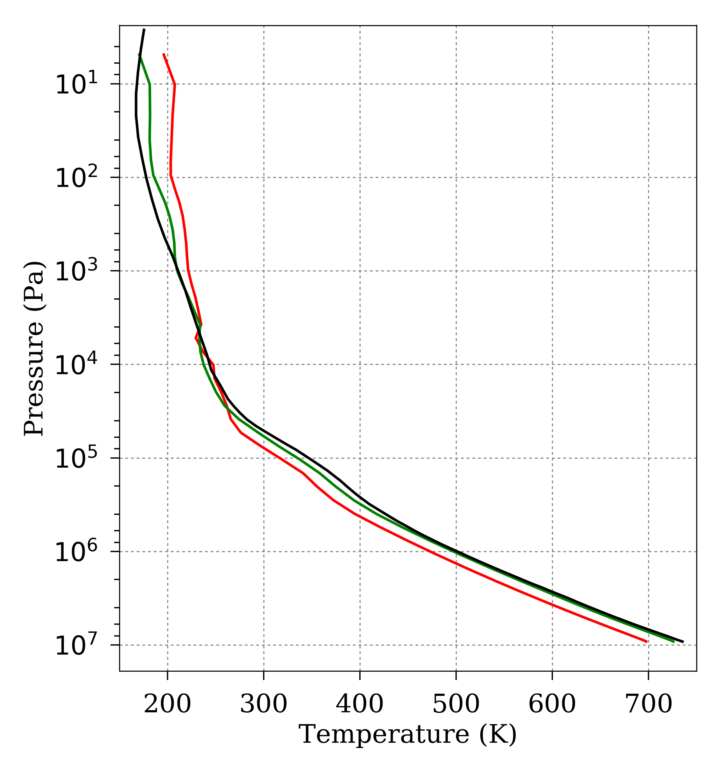
Figure 1: Horizontally and temporally averaged temperature profile for the previous (red) and current (green) IPSL Venus GCM models at the end of simulation (300 Vd) compared to VIRA reference profile (black). Data is globally averaged over all longitudes and latitudes in each altitude, and over 2 Vd in time.

As a direct consequence of the above described modifications done in the radiative transfer (considering both stages), the average temperature field has significantly improved. The horizontally and temporally averaged temperature profile is now (varcld simulation mentioned above) closer to the VIRA profile (see Figure 1) with warmer modeled temperatures below the clouds (and colder above) than in the previous model (Lebonnois et al.,, 2016). In the 3-dimensional simulations presented here, and compared to the 1-dimensional tests performed in Lebonnois and Schubert, (2017) (Methods and Supplementary Information), the average temperature field is still approximately 10 K colder than observed below roughly 70 km. However, due to the sensitivity to the solar heating rates below the clouds and the associated uncertainties, no additional tuning was performed.

FIG 1

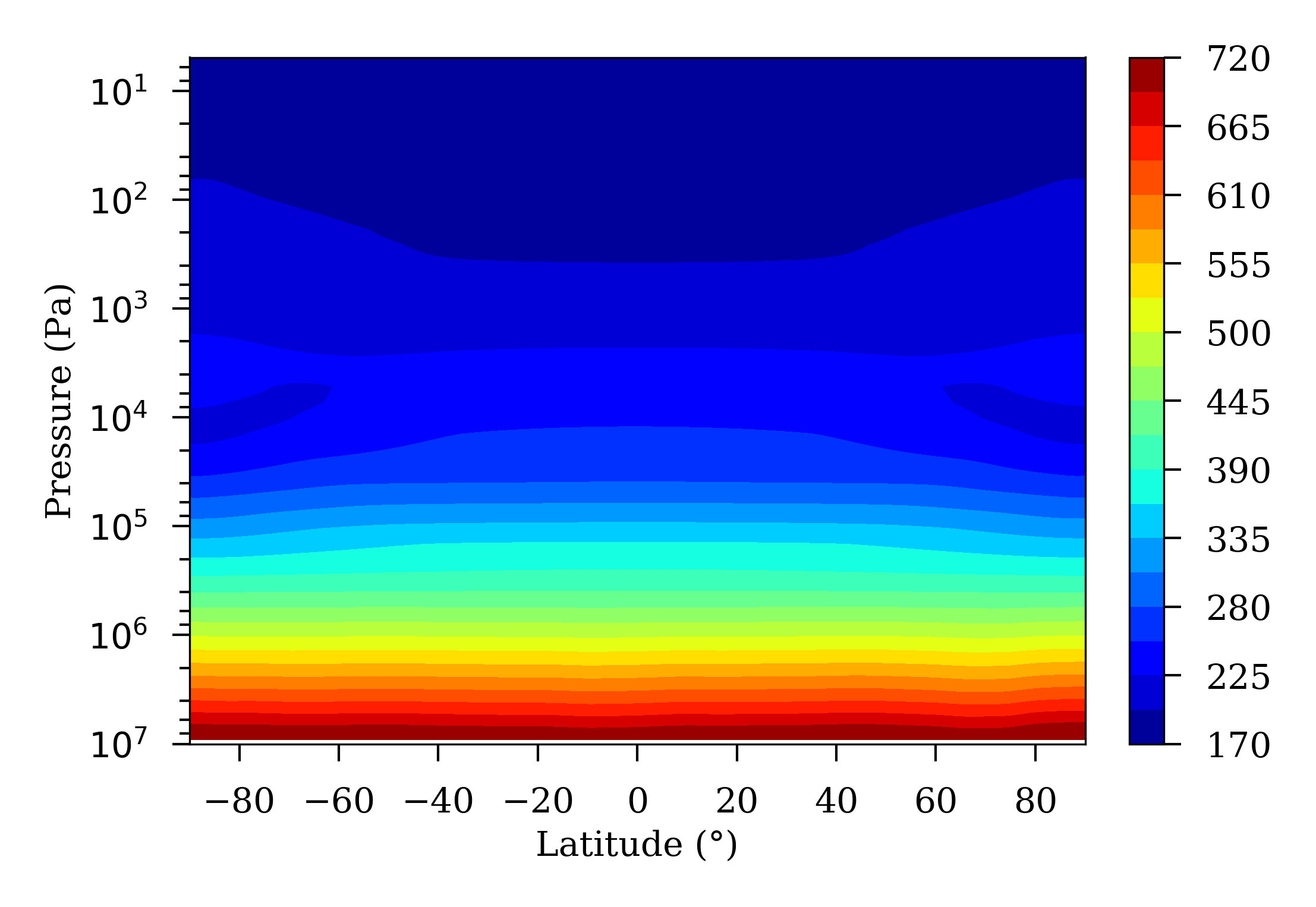
Figure 2: Zonally and temporally averaged temperature field (K) for the current IPSL Venus GCM model at the end of simulation (300 Vd). Data is averaged over $360\degree$ in longitude and 2 Vd in time.

The altitude-latitude distribution of the zonally and temporally averaged temperature (Figure 2) shows two clearly differentiated behaviors. Above $4\times 10^{3}$ Pa the temperature increases from equator to pole, but below $2\times 10^{4}$ Pa it smoothly decreases towards the pole, just as seen in observation-based maps (e.g. Tellmann et al.,, 2009; Haus et al.,, 2014). Moreover, a new structure that resembles clearly the cold collar appears for the first time in the IPSL Venus GCM, at $2\times 10^{4}-4\times 10^{3}$ Pa ($\sim 62-66$ km) altitude and between $60\degree$ and $90\degree$ in both hemispheres. This feature is not isolated from the pole as in the observation-based maps, but it is the most similar feature reproduced so far. The temperature values obtained with our model ($\sim$220 K) are in good agreement with observations. Therefore, the latitudinal variation of the clouds’ structure plays a key role in the formation of the cold collar. The development of the cold collar related to the radiative transfer in the polar atmosphere of Venus is discussed in detail below (Section 4).

FIG 2

3.2 Cold collar

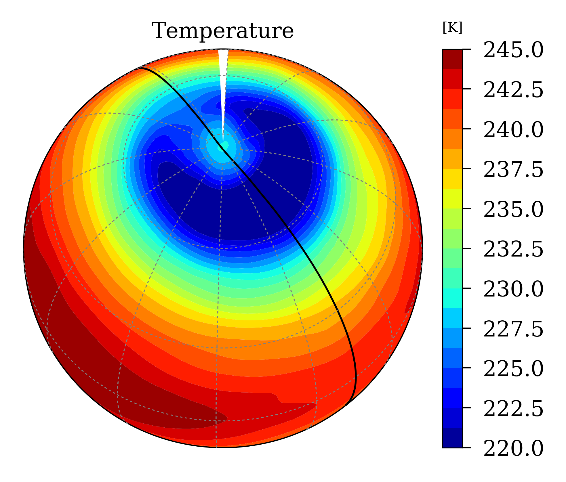
Figure 3: Example of polar temperature field at $7\times 10^{3}$ Pa ($\sim$64 km) for the current IPSL Venus GCM model. Temperature is averaged over 1/24 Vd $\sim$ 4.88 Earth days. Black line shows the terminator with dayside on front.

Figure 3 shows an example of the temperature field at the northern pole at $7\times 10^{3}$ Pa ($\sim$64 km) altitude. The atmosphere between $60\degree$ and $85\degree$ is clearly colder than the rest of the latitudes, being on average $\sim$20 K colder than the equator and about 10 K colder than the pole. The coldest region seen close to the terminator shows values about 220 K, in good agreement with values observed by VIRTIS (e.g. Haus et al.,, 2014; Garate-Lopez et al.,, 2015). The inner warm core shows an average value of 230 K (colder than the observed mean values). However, we find values as high as 240 K in about $3\%$ of the time over the last simulated 2 Vd.

FIG 3

The temporal evolution of the polar temperature obtained by our current model does not always show an inner region surrounded by the cold collar and the structure simulated within the inner core is smoother than obtained by Yamamoto and Takahashi, (2015) and Ando et al., (2016, 2017) (these GCMs use spectral dynamical cores that do not have singularities at the pole). The altitude level where the cold collar is reproduced ($\sim$64 km) and the temperature values ($\sim$220 K) obtained by the IPSL Venus GCM are, however, more consistent with observations (e.g. $\sim$62 km and $\sim$220 K by Tellmann et al., 2009).

The coldest region shows a rotation around the pole with a period of about 5.85 Earth days in the model, that agrees with the 5 - 10 Earth days period found by (Luz et al.,, 2011) for the drift of the rotation center of the vortex around the pole. However, the modeled inner core does not show a clear rotation around the pole, so it is difficult to compare its motion to the one observed for the warm vortex (Luz et al.,, 2011; Garate-Lopez et al.,, 2013).

Figure 3 in Lebonnois et al., (2016) displayed four temperature fields at pressure $3\times 10^{3}$ Pa ($\sim$67 km) in the northern polar region that showed a cold polar region with an inner warmer core. The altitude level where these features are obtained is slightly different comparing the previous and current models but the horizontal structure simulated in both cases is very similar in general, probably due to the longitudinal polar filter of the model that does not allow to reproduce fine-scale features.

3.3 Average wind field

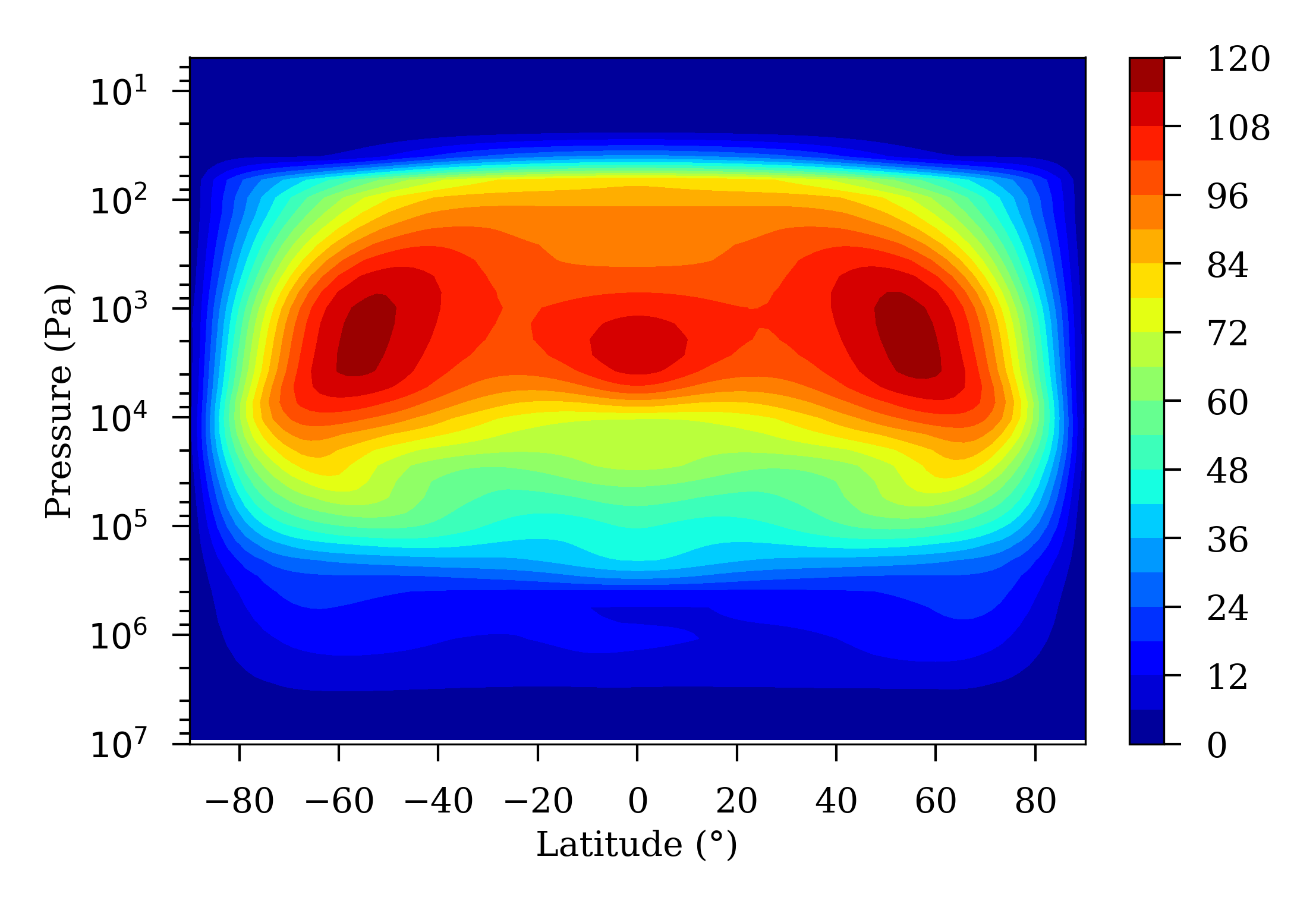
Figure 4: Zonally and temporally averaged zonal wind field for the current IPSL Venus GCM model at the end of simulation (300 Vd). Data is averaged over $360\degree$ in longitude and 2 Vd in time.

Considering the latitudinal structure of the clouds has also improved the zonally and temporally averaged zonal wind field. The modeled equatorial jet is now less intense than the mid-latitude jets (Figure 4) as cloud-tracking measurements suggest (Hueso et al.,, 2015). The modeled mid-latitude jets are still located too close to the poles (and, therefore, the latitudinal wind gradient is still high poleward of $70\degree$) but their altitude has gone down slightly, while the equatorial jet has ascended a bit.

FIG 4

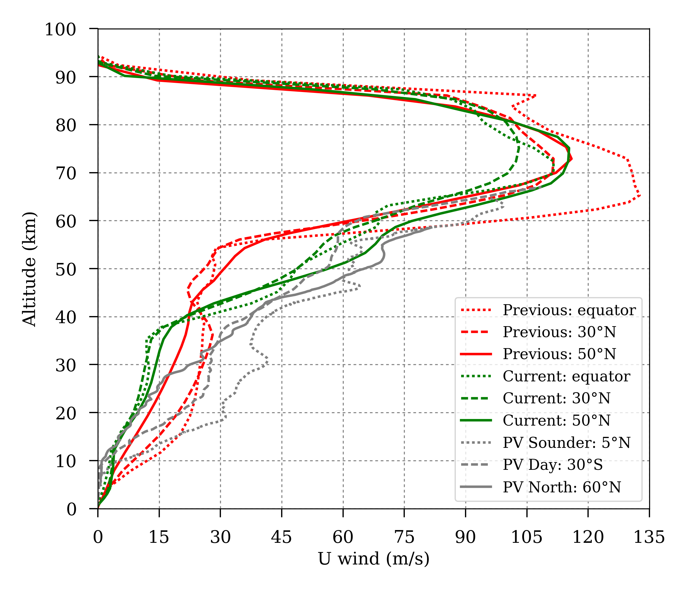
Figure 5: Vertical profiles of the zonally and temporally averaged zonal wind at different latitudes for the previous (red) and current (green) IPSL Venus GCM models at the end of simulation (300 Vd). Data is averaged over $360\degree$ in longitude and 2 Vd in time. Measurements from different Pioneer Venus probes are added in gray.

In the previous model (Lebonnois et al.,, 2016) winds at 40 - 60 km were approximately half of the observed values, but the currently modeled winds at this altitude range are on average $\sim 20~{}m/s$ (about $75\%$) faster and are now in good agreement with the Venera and Pioneer Venus probes’ profiles (see Figure 5). According to a new wave activity analysis that is still on-going work and will be presented in a subsequent publication, this improvement of the averaged zonal wind could be due to a new baroclinic activity found between 40 and 60 km altitude and that transports heat and angular momentum equatorwards. Nevertheless, the velocity of the zonal winds below 40 km altitude has decreased showing winds significantly slower than observed, which was not the case previously. The large-scale gravity waves present in the deep atmosphere in the previous simulation (Lebonnois et al.,, 2016) are no longer obtained, which probably explains this worsening in the zonal wind below 40 km.

FIG 5

4 Cold Collar Analysis

To analyze in detail the influence of the latitudinal structure of the clouds in the formation of the cold collar, the simulation with the latitudinal variations of the cloud structure (varcld simulation) is compared to a control simulation in which a uniform cloud structure is maintained in the IR cooling computation (unifcld simulation). Note that the simulations differ in the second stage of the implementation (see Section 2.1), i.e. in the last 100 Vd, so the solar heating rates take into account the latitudinal variations in both simulations (same look-up table). The unifcld simulation has no physical sense since the cloud model is different in the solar heating and IR cooling treatments, and its results are very similar to the previous simulation presented by Lebonnois et al., (2016), but we think that the comparison between unifcld and varcld simulations is useful to identify which are the key elements in the formation of the cold collar.

The cold collar is formed in the varcld simulation but not in the unifcld simulation, which indicates that the generation of this characteristic feature is not affected by latitudinal variations of the clouds in the solar heating rates. It is the influence that the cloud structure has in the IR cooling rates that forms the cold collar.

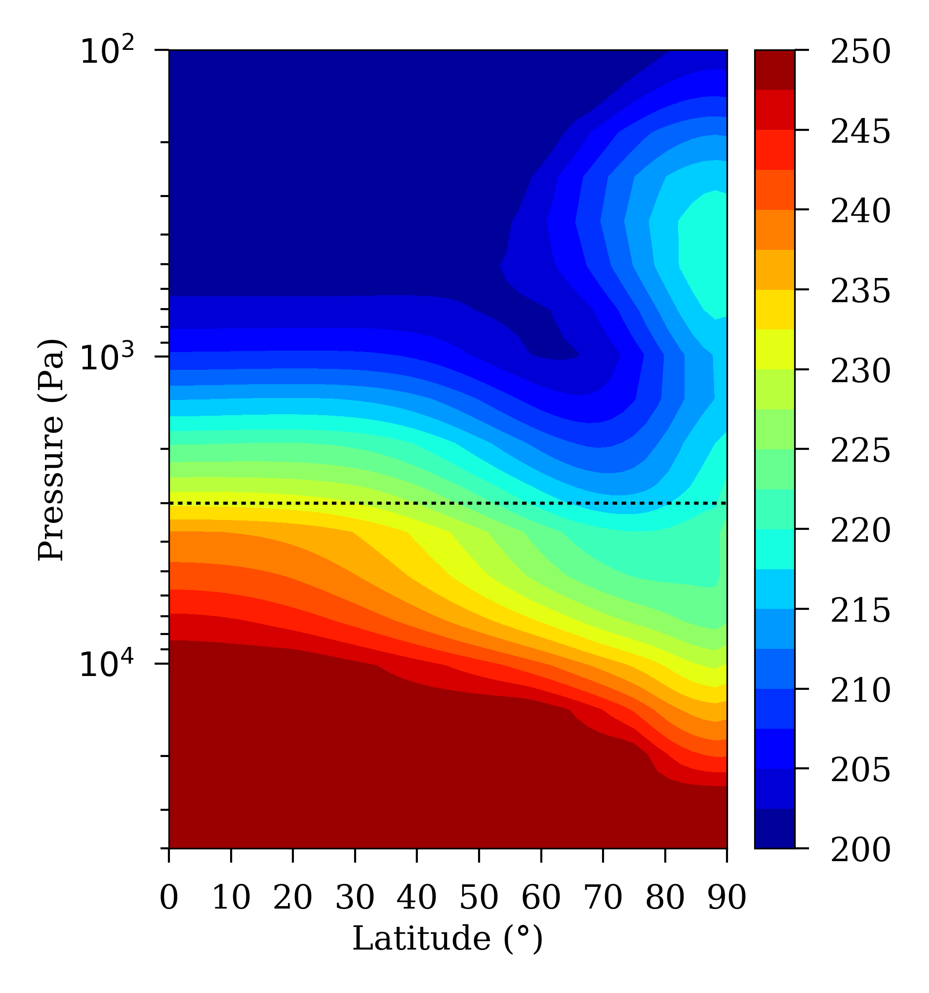
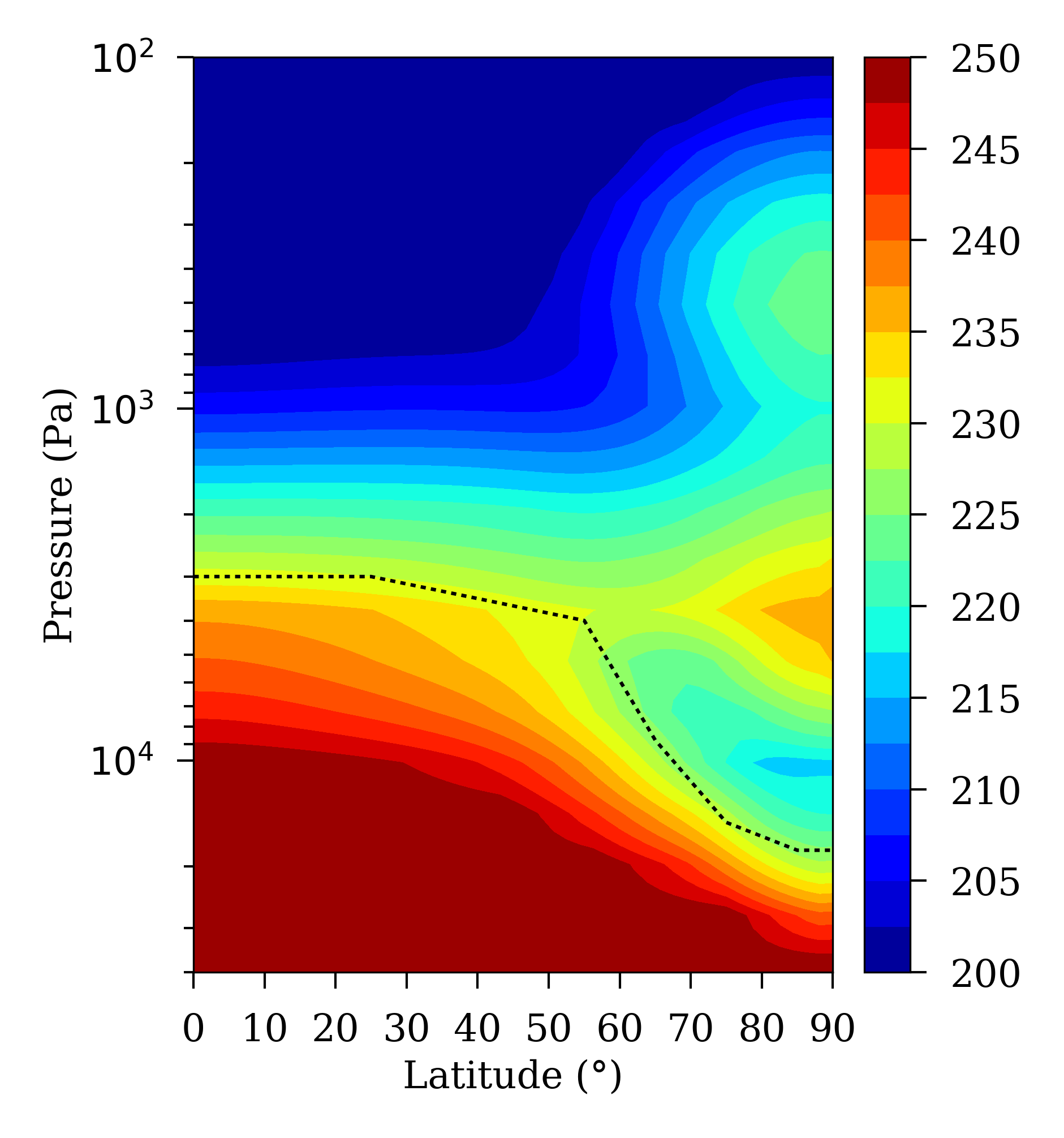
Figure 6: Zonally and temporally averaged temperature field (K) obtained at the end of simulation (300 Vd) when considering uniform (left) and variable (right) clouds in the IR cooling computation during the last 100 Vd. Data is averaged over $360\degree$ in longitude and 2 Vd in time. Dashed line shows the cloud top altitude at 1 $\mu$m corresponding to the Haus et al., (2014) cloud model.

In the unifcld simulation (Figure 6a), there is a cold region around $10^{3}$ Pa and $65\degree$ that extends downward and poleward, creating a warmer region close to the pole and above that altitude level, but this cold feature is not exactly as the one observed (e.g. Tellmann et al.,, 2009; Haus et al.,, 2014), it is not completely surrounded by warmer air. This structure, as well as the global thermal structure in the unifcld simulation, is very similar to the structure obtained in previous works and presented there as the cold collar (Ando et al.,, 2016, 2017; Lebonnois et al.,, 2016). The relation between this structure and the thermal tides in the polar atmosphere was demonstrated by Ando et al., (2016) and it should be similar in the unifcld simulation presented here.

FIG 6

On the other hand, the cold feature seen in the average temperature map that corresponds to the varcld simulation resembles significantly more to the observed cold collar, being more contrasted from the surrounding warmer atmosphere and located at the correct altitude and latitude. It is not completely isolated which is a characteristic different from observations. It is connected to the pole at an altitude of about $10^{4}$ Pa ($\sim$62 km) and then extends upward and equatorward. However, the connection to the pole is most likely related to the grid used currently in the model which is based on a longitude-latitude scheme with a longitudinal polar filter that reduces the latitudinal resolution and removes the high frequency variations in the polar regions. So the results at latitudes higher than $80\degree$ should be taken with caution. A new icosahedral dynamical core (Dubos et al.,, 2015) will be used in the near future that should improve the robustness of the computation of the polar circulation. This should affect the fine structure of the cold collar and the inner warm core (at about $4\times 10^{3}$ Pa and $80\degree$ - $90\degree$).

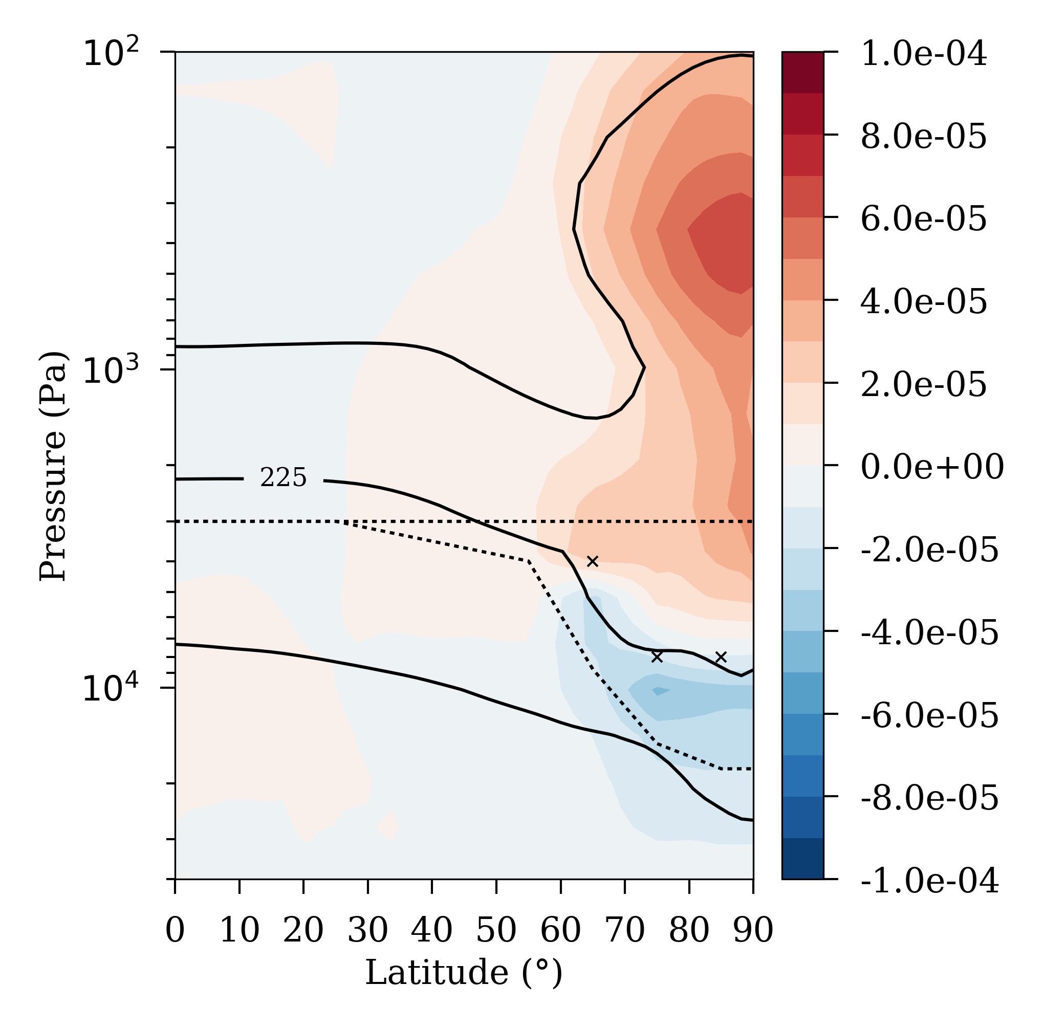
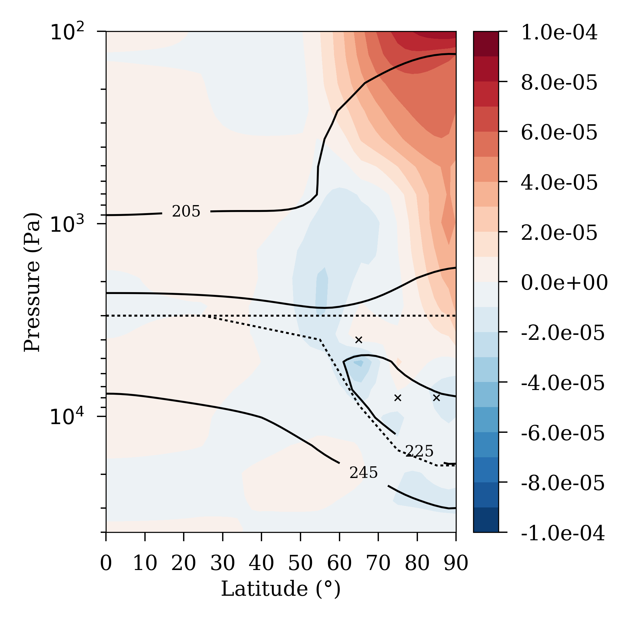
Figure 7: Difference of the IR cooling rates (K/s) between the varcld and unifcld simulations as soon as the latitudinal cloud structure is implemented in the IR cooling computation (a, 0.01 Vd, instantaneous field) and 100 Vd after (b, field averaged over 2 Vd). Data is averaged over $360\degree$ in longitude. Solid lines show 205K, 225K, and 240K temperature contours of the varcld simulation (unifcld simulation’s temperature field at 0.01 Vd is the same as the varcld simulation and 100 Vd after is very similar to that at 0.01 Vd). Dotted lines show the cloud top at 1 $\mu$m for the uniform and variable cloud models. Crosses show the cloud upper altitude boundary (see text).

To confirm the dominant influence of the cloud structure on the IR cooling and on the temperature field, the IR cooling rates of both unifcld and varcld simulations are compared. Figure 7 shows the difference between varcld and unifcld IR cooling (IR_varcld - IR_unifcld) at the first timestep of the simulations after the new cloud model is implemented in the IR cooling computation (0.01 Vd), so that the background temperature field has not changed and is the same for both simulations, and after 100 Vd, at the end of simulations. Note that the negative values in Figure 7 mean IR cooling is stronger in the varcld simulation while positive values mean it is stronger in the unifcld simulation. The unit used in the Figure is K/s, so that $1\times 10^{-4}$ K/s corresponds to $\sim$8.64 K/Earth day. This is in good agreement with Lee and Richardson, (2011) who states that the IR cooling exceeds 10 K/Ed only above 100 Pa.

FIG 7

From the very first moment when the cloud’s latitudinal structure is taken into account in the IR radiation computation, unifcld and varcld simulations evolve in a completely different way with no possible convergence. The atmosphere at the varcld simulation develops a stronger cooling region around $75\degree$ latitude and $10^{4}$ Pa altitude. It also develops a weaker cooling region around $85\degree$ latitude and $4\times 10^{2}$ Pa altitude. During tens of Venusian days the polar atmosphere evolves in such a way that after 60 Vd it reaches a new equilibrium, although the average temperature at the cold collar oscillates slightly afterwards. Figure 7b shows that the stronger and weaker cooling regions in the varcld simulation are still present 40 Vd after reaching the equilibrium, at 100 Vd. This is important because it means that the atmosphere at the newly formed cold collar will be constantly cooling by means of IR radiation in a quite stronger way than the atmosphere above it (referred to as the warm mesospheric pole hereon). As long as this new equilibrium endures, the cold collar will remain colder than its surroundings due to this stronger IR cooling.

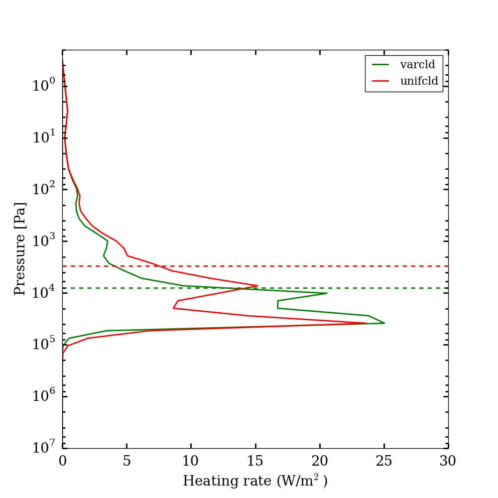
Figure 8: IR energy exchanges between each layer and space at $75\degree$ latitude at the end of simulation (300 Vd, profiles averaged over $360\degree$ in longitude and 2 Vd in time) when considering uniform (red, unifcld) and variable (green, varcld) clouds in the IR cooling computation during the last 100 Vd. Red dashed line indicates the 1 $\mu$m cloud-top level in the unifcld simulation, while the green dashed line indicates the cloud upper altitude boundary in the varcld simulation.

Figure 8 displays the vertical profile of the IR energy exchange between different atmospheric levels and space for both unifcld and varcld simulations at the end of simulation (100 Vd) and at $75\degree$ latitude (cold collar region). The energy loss to space from the upper clouds ($\sim$50 - 70 km altitude) is more localized in altitude in the varcld simulation than in the unifcld simulation. This, as well as the decay rate of the cooling with altitude above the clouds, is inherited from the cloud model by Haus et al., (2014). At high-latitude (higher than $60\degree$) the retrieval of the cloud top altitude required the estimation of another quantity, the cloud upper altitude boundary, above which no cloud particles are considered. This cloud upper altitude boundary (located slightly above the cloud top defined at 1 $\mu$m) strongly affects the highest peak in the cooling rates, intensifying it. This peak corresponds mainly to the cooling rates in the 6-12 $\mu$m range and it is associated to the uppermost layer of cloud particles in the model. The lowest peak in the vertical profiles of Figure 8 corresponds mostly to the cooling at 20-30 $\mu$m and is associated to the base of the upper clouds, while the cooling above the clouds occurs mainly in the aisles of the 15 $\mu$m band (Lebonnois et al.,, 2015).

FIG 8

The position of the cold collar with respect to the cloud top (defined at 1 $\mu$m) and the cloud upper boundary is better seen in Figure 7. It is located just in between, coinciding with the highest peak of the cooling rates in the vertical profile. This means that the opacity at 1 $\mu$m equals unity within the upper clouds, but that there is a region with cloud particles above it where the cold collar is formed. The cold collar is, therefore, located at the uppermost layer of the clouds. Its position is, however, cloud model dependent since it is strongly linked to the cloud upper boundary defined by Haus et al., (2014).

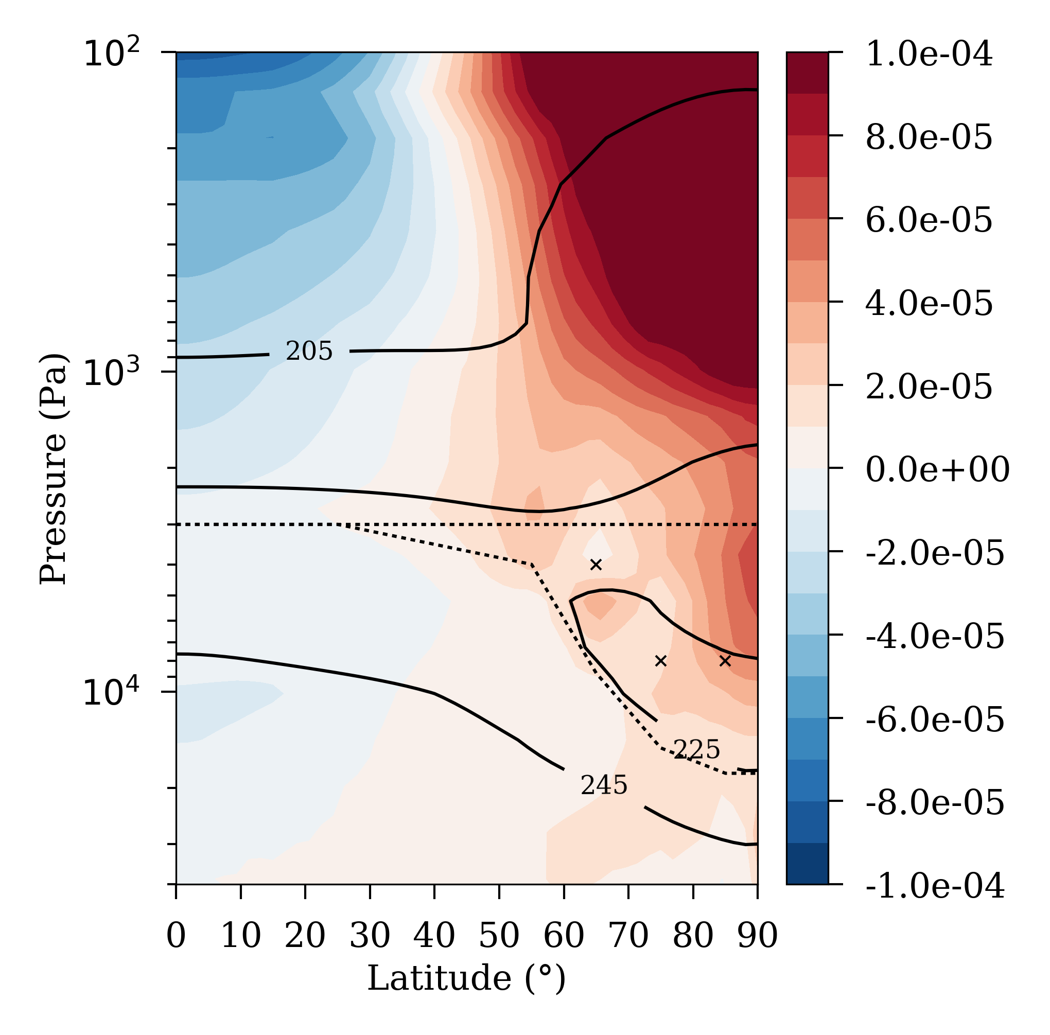
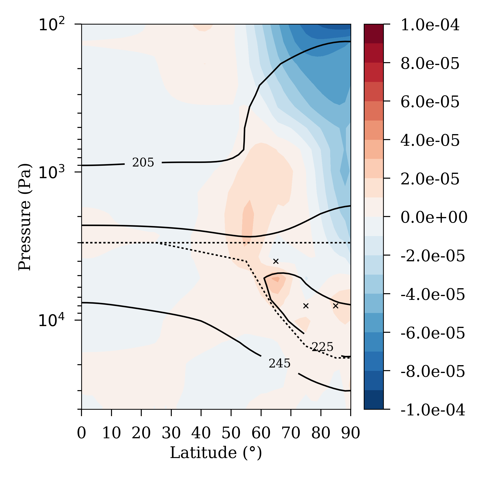
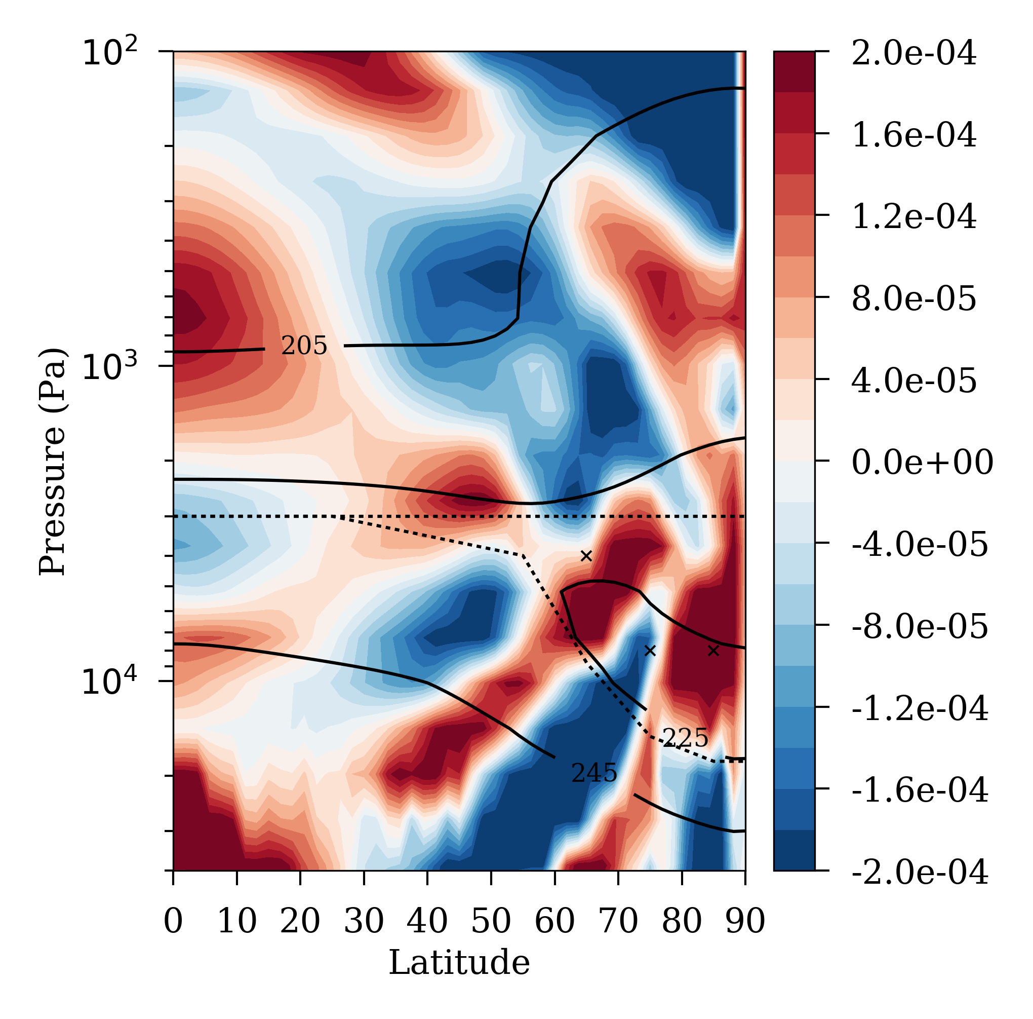
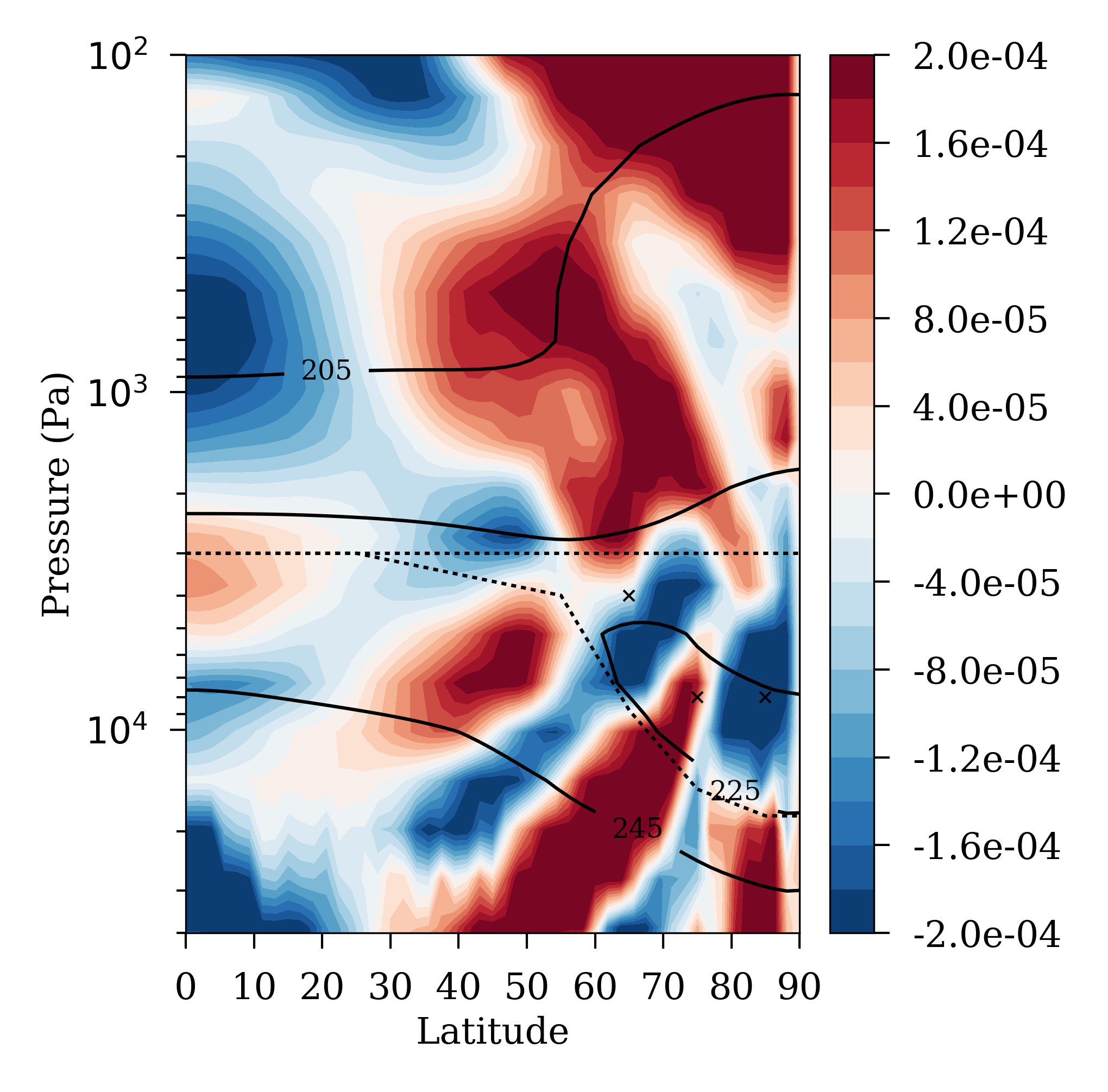
Figure 9: (a) dynamical heating in the varcld simulation, (b) difference of the dynamical heating between varcld and unifcld simulations, (c) horizontally and (d) vertically transported dynamical heating in the varcld simulation. All fields are plotted after 100 Vd with the latitudinal cloud structure implemented (varcld) or not (unifcld) in the IR cooling computation and are averaged over $360\degree$ in longitude and 2 Vd in time. Solid lines, dotted lines and crosses: same as in Fig. 7. Units: K/s.

The induced modifications in the temperature structure affects the circulation and the thermal energy transport, both horizontally and vertically. A detailed analysis of the new dynamical state of the polar atmosphere and of the transport of heat and angular momentum is beyond the scope of the present paper, but the tendencies in the temperature fields due to dynamical heat transport are analyzed here to better understand the new equilibrium in which the cold collar is formed. The heating/cooling rates due to the dynamics in the varcld simulation can be seen in Figure 9a. Dynamics is globally cooling the low-latitudes and heating the polar regions, as in the simulation with uniform cloud model and previous simulations (not shown here). Figure 9b shows the dynamical heating difference between unifcld and varcld simulations with positive values meaning stronger heating in the varcld simulation. Not surprisingly, it is the inverse of Figure 7b since dynamical heating should compensate the radiative cooling in order to have an atmosphere in thermal equilibrium. Actually, in the cold collar area this heating due to dynamics is slightly stronger in the varcld simulation than in the unifcld simulation to compensate the excess of IR cooling. And in the warm pole, including the warm mesospheric pole ($85\degree$ latitude and $4\times 10^{2}$ Pa) and the inner warm core ($85\degree$ latitude and $4\times 10^{4}$ Pa), the dynamical heating is weaker due to the weaker IR cooling there.

FIG 9

In Figures 9c and 9d dynamical heating in the varcld simulation is separated between horizontally and vertically transported heating. In both panels heating is represented by red colors (positive values) and the cooling due to dynamics by blue colors (negative values). The atmosphere shows a patchy structure with dynamical heating and cooling regions interspersed with each other in both horizontal and vertical terms. These two terms are inversely related; regions where the horizontal dynamics heats the atmosphere are cooled by vertical dynamics, and vice versa. However, recall that the effects of taking into account the latitudinal variations of the clouds take place in the cold collar and warm pole areas (Figure 9b), where dynamics heats the atmosphere (Figure 9a). Above the clouds, in the warm mesospheric pole, the polar heating due to dynamics occurs by means of vertical transport (Figure 9d), but it is mitigated by horizontal transport (Figure 9c). On the other hand, in the cold collar and inner warm core areas, horizontal transport mostly heats the area (although a region of dynamical cooling is appreciated between the main two heating regions). This heating is mitigated by vertical heating transport.

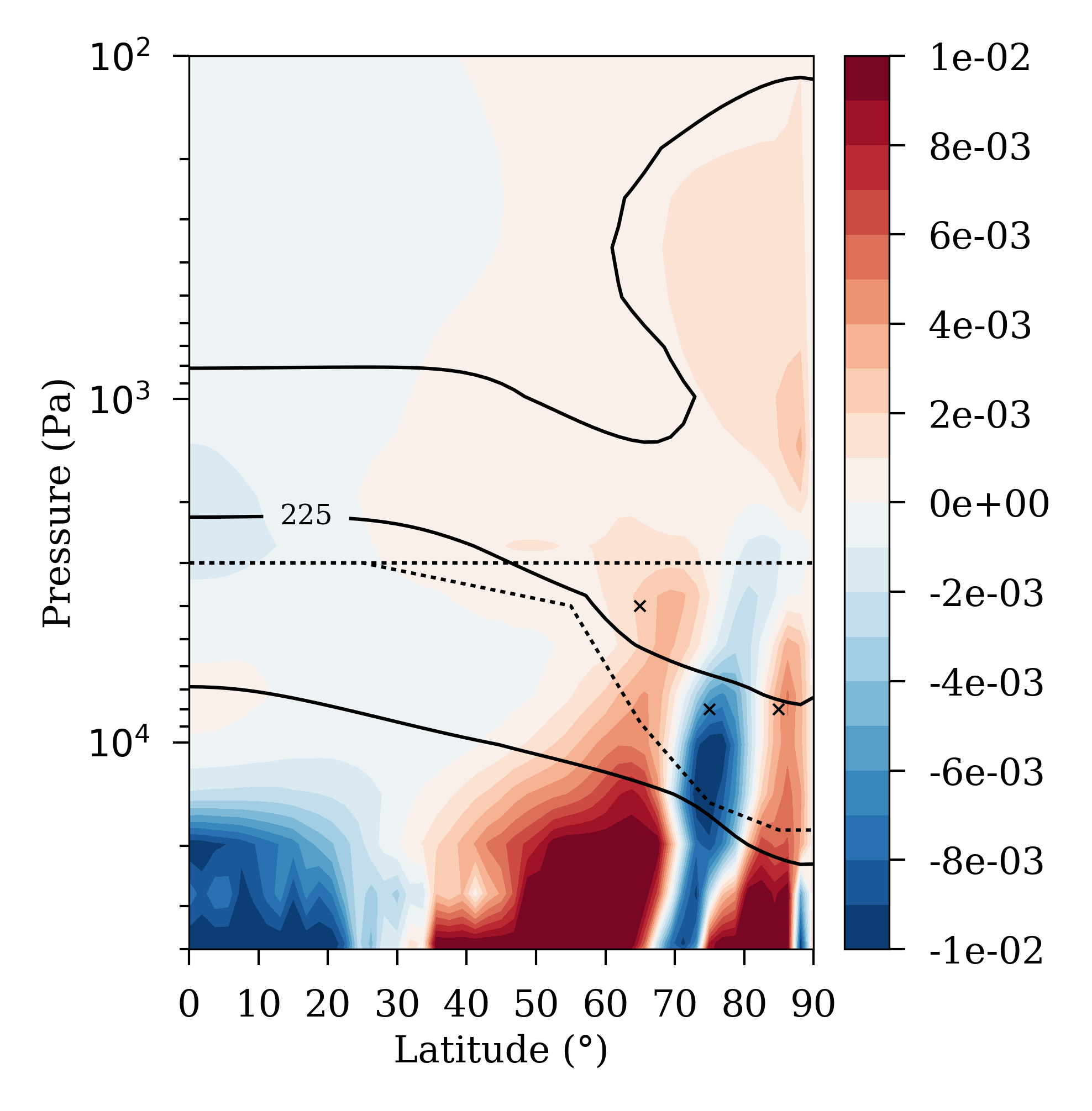
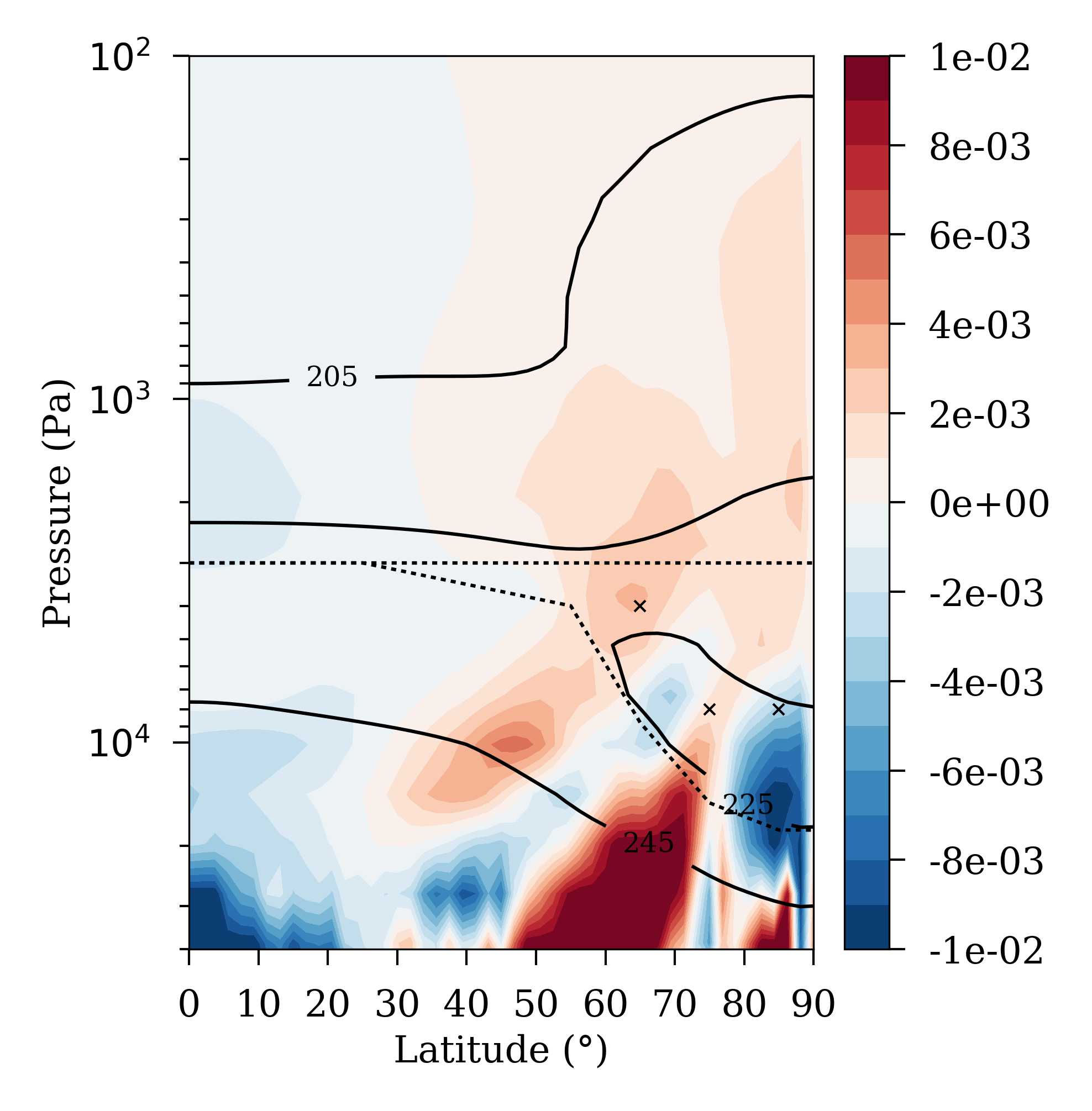
Figure 10: Zonally and temporally averaged vertical wind velocity (Pa/s) at the end of simulation (300 Vd), when considering uniform (a) and variable (b) clouds in the IR cooling computation during the last 100 Vd. Data is averaged over $360\degree$ in longitude and 2 Vd in time. Solid lines, dotted lines and crosses: same as in Fig. 7.

Studying the variation of the circulation, particularly of the zonal and meridional winds, is not trivial due to the high variability present in the polar regions. This study of the horizontal distribution of the dynamical polar atmosphere in the varcld simulation will be presented in a subsequent paper together with the new wave activity. However, the variation of vertical wind is interesting and noteworthy. Figure 10 shows the vertical wind velocity fields in both unifcld and varcld simulations (in Pa/s units, so negative values mean upwelling motion). Although the main differences take place at the clouds and levels below, an altered subsidence structure that extends down to $50\degree$ latitude is seen in the varcld simulation, responsible of the vertical heating seen in Figure 9d. Ascending air is found in the cold collar between $60\degree$ and $70\degree$ latitudes and at about $10^{4}$ Pa altitude for the varcld simulation which is associated with the dynamical cooling seen in Figure 9d. A reversal of the vertical circulation in the $70\degree$ - $90\degree$ polar region from unifcld to varcld simulations is also clearly seen.

FIG 10

Hence, according to the results of the new IPSL Venus GCM, the cold collar feature observed in Venus’ polar atmosphere is formed by the infrared cooling region generated by the decrease of the cloud top altitude poleward and the latitudinal variation of the particles modes. Since the radiative forcing cools the area while the dynamics heats it, resulting in a region characteristically cold, it seems that the driver of the cold collar is the radiative transfer rather than dynamics. However, the presence of the cold collar strongly influences the dynamics, thus affecting the polar circulation of Venus. Even though the cloud distribution, radiative transfer, and dynamics form a coupled system in reality and, therefore, any change in one of the mentioned aspects will bring along a change in the other aspects, this coupling is not yet present in our GCM and we can not characterize it in detail.

The temporal evolution observed in the modeled polar temperature maps at $7\times 10^{3}$ Pa altitude (not shown here) presents a cold collar that is displaced from the pole and rotates around it. The obtained rotation period of 5.85 Earth days agrees with the period found by Luz et al., (2011) for the drift of the rotation center of the vortex around the pole. This result, together with the structure of the cold feature in the average temperature field, indicates that the current IPSL Venus GCM models satisfactorily the subpolar latitudes. However, the current polar latitudes’ treatment is not ideally suited and, therefore, the modeled inner core does not show neither a clear rotation around the pole nor detailed horizontal structure within it, as the observed polar vortex does.

5 Conclusions

The previous IPSL Venus GCM (Lebonnois et al.,, 2016) has been modified in order to improve the radiative transfer, update the cloud model, and take into account the latitudinal variation of the clouds (by means of cloud top altitude and different modes’ abundances) in the solar heating profiles and infrared cooling computation. The new cloud model used in the current version is described by Haus et al., (2014) and shows that the cloud top altitude decreases towards the pole in Venus’s atmosphere and that the different particle modes’ abundances change from equator to pole.

The zonally and temporally averaged zonal wind and temperature fields have been improved showing now a better agreement with the observations. Particularly, the equatorial jet’s intensity has decreased compared to the mid-latitude jets’ intensity, the zonal wind velocities between 40 and 60 km altitude are faster than previously, and the averaged temperature values below (resp. above) the clouds are now warmer (resp. colder), thus closer to the VIRA reference profile.

The main result, however, is the appearance of a feature in the averaged altitude-latitude temperature map that resembles the subpolar cold collar observed in Venus’s atmosphere. The atmosphere between $60\degree$ and $85\degree$ shows a thermal minimum at $2\times 10^{4}-4\times 10^{3}$ Pa ($\sim 62-66$ km) altitude, being $\sim$20 K colder than the equator and about 10 K colder than the pole. The coldest region shows values about 220 K, in good agreement with observed values, but the inner warm core shows an average value of 230 K that is colder than the observed values. The structure simulated within the inner core is smoother than that obtained by Yamamoto and Takahashi, (2015) and Ando et al., (2016, 2017), but the altitude level where the cold collar is reproduced and the modeled temperature values are more consistent with observations.

According to our analysis the cloud’s latitudinal structure is an essential element in the formation of the cold collar via the IR cooling rates. A strong cooling region at $\sim 75\degree$ and $10^{4}$ Pa is developed as soon as the new cloud structure is implemented in the IR computations and it remains cooling strongly after a new equilibrium is reached and the cold collar is formed. A region of weak IR cooling is also developed above the polar clouds just where the warm mesospheric pole is observed.

The position of the cold collar is cloud model dependent since it is strongly linked to the cloud upper altitude boundary (level above which no particles are considered) defined by Haus et al., (2014) at high latitudes. The IR cooling peak is located right below this cloud upper boundary, above the cloud top altitude. This means that the cold collar is located at the uppermost layer of the clouds, in a region with cloud particles but above the level where the opacity equals one at 1 $\mu$m.

Once the atmosphere reaches a new thermal equilibrium, the radiative cooling is compensated by heating due to dynamics. Consequently, the dynamical heating is stronger at the cold collar area than in the warm mesospheric pole ($85\degree$ and $4\times 10^{2}$ Pa). Our analysis points to vertical transport (associated to a subsidence motion that extends down to $50\degree$) as the main source of dynamical heating in the warm mesospheric pole and to horizontal transport at the cold collar.

Since the radiative forcing cools the area while the dynamics heats it, resulting in a region characteristically cold, it seems that the driver of the cold collar is the radiative transfer rather than dynamics.

Table 1: Chosen inputs for the simulations.

	Solar heating		Correlated-k set		Cloud model (IR)			Continuum (3-7$\mu m$)
	C86a	H15b	L16c	updated	Z07d	H13e	H14f	L16c	updatedg
Initial state	$\times$		$\times$		$\times$			$\times$
0-200 Vd		$\times$	$\times$			$\times$			$\times$
200-300 Vd:
- unifcld		$\times$		$\times$		$\times$			$\times$
- varcld		$\times$		$\times$			$\times$		$\times$

^a Crisp, (1986)
^b Haus et al., (2015), with additional tuning in lower haze area (see text)
^c Lebonnois et al., (2016)
^d Zasova et al., (2007)
^e Haus et al., (2013), clouds taken as uniform with latitude
^f Haus et al., (2014), clouds taken as variable with latitude
^g see text

References

- Ando et al., (2017) Ando, H., Imamura, T., Sugimoto, N., Takagi, M., Kashimura, H., Tellmann, S., Pätzold, M., Häusler, B., and Matsuda, Y. (2017). Vertical structure of the axi-asymmetric temperature disturbance in the Venusian polar atmosphere: comparison between radio occultation measurements and GCM results. J. Geophys. Res. Planets, 122:1687–1703.
- Ando et al., (2016) Ando, H., Sugimoto, N., Takagi, M., Kashimura, H., Imamura, T., and Matsuda, Y. (2016). The puzzling Venusian polar atmospheric structure reproduced by a general circulation model. Nature Comm., 7:10398.
- Belton et al., (1976) Belton, M. J. S., Smith, G. R., Schubert, G., and del Genio, A. D. (1976). Cloud patterns, waves and convection in the Venus atmosphere. J. Atm. Sci., 33:1394–1417.
- Crisp, (1986) Crisp, D. (1986). Radiative forcing of the Venus mesosphere. I - Solar fluxes and heating rates. Icarus, 67:484–514.
- Del Genio and Rossow, (1990) Del Genio, A. D. and Rossow, W. B. (1990). Planetary-scale waves and the cyclic nature of cloud top dynamics on Venus. J. Atmos. Sci., 47:293–318.
- Dubos et al., (2015) Dubos, T., Dubey, S., Tort, M., Mittal, R., Meurdesoif, Y., and Hourdin, F. (2015). DYNAMICO-1.0, an icosahedral hydrostatic dynamical core designed for consistency and versatility. Geosci. Model Dev., 8:3131–3150.
- Eymet et al., (2009) Eymet, V., Fournier, R., Dufresne, J.-L., Lebonnois, S., Hourdin, F., and Bullock, M. A. (2009). Net-exchange parameterization of the thermal infrared radiative transfer in Venus’ atmosphere. J. Geophys. Res., 114:E11008.
- Garate-Lopez et al., (2015) Garate-Lopez, I., García Muñoz, A., Hueso, R., and Sánchez-Lavega, A. (2015). Instantaneous three-dimensional thermal structure of the South Polar Vortex of Venus. Icarus, 245:16–31.
- Garate-Lopez et al., (2013) Garate-Lopez, I., Hueso, R., Sánchez-Lavega, A., Peralta, J., Piccioni, G., and Drossart, P. (2013). A chaotic long-lived vortex at the southern pole of Venus. Nature Geosci., 6:254–257.
- Gierasch, (1975) Gierasch, P. (1975). Meridional circulation and the maintenance of the Venus atmospheric rotation. J. Atmos. Sci., 32:1038–1044.
- Gierasch et al., (1997) Gierasch, P. J. et al. (1997). The general circulation of the Venus atmosphere: an assessment. In S. W. Bougher, D. M. Hunten and R. J. Phillips, editor, Venus II, geology, geophysics, atmosphere, and solar wind environnement, pages 459–500. Univ. of Arizona Press.
- Grassi et al., (2010) Grassi, D., Migliorini, A., Montabone, L., Lebonnois, S., Cardesin-Moinelo, A., Piccioni, G., Drossart, P., and Zasova, L. V. (2010). The thermal structure of Venusian night-time mesosphere as observed by VIRTIS-Venus Express. J. Geophys. Res., 115:E09007.
- Grassi et al., (2014) Grassi, D., Politi, R., Ignatiev, N. I., Plainaki, C., Lebonnois, S., Wolkenberg, P., Monatbone, L., Migliorini, A., Piccioni, G., and Drossart, P. (2014). The Venus nighttime atmosphere as observed by VIRTIS-M instrument. Average fields from the complete infrared data set. J. Geophys. Res. Planets, 119:837–849.
- Haus et al., (2013) Haus, R., Kappel, D., and Arnold, G. (2013). Self-consistent retrieval of temperature profiles and cloud structure in the northern hemisphere of Venus using VIRTIS/VEX and PMV VENERA-15 radiation measurements. Planet. & Space Sci., 89:77–101.
- Haus et al., (2014) Haus, R., Kappel, D., and Arnold, G. (2014). Atmospheric thermal structure and cloud features in the southern hemisphere of Venus as retrieved from VIRTIS/VEX radiation measurements. Icarus, 232:232–248.
- Haus et al., (2015) Haus, R., Kappel, D., and Arnold, G. (2015). Radiative heating and cooling in the middle and lower atmosphere of Venus and responses to atmospheric and spectroscopic parameter variations. Planet. & Space Sci., 117:262–294.
- Hourdin et al., (2006) Hourdin, F., Musat, I., Bony, S., Braconnot, P., Codron, F., Dufresne, J.-L., Fairhead, L., Filiberti, M.-A., Friedlingstein, P., Grandpeix, J.-Y., Krinner, G., Levan, P., Li, Z.-X., and Lott, F. (2006). The LMDZ4 general circulation model: climate performance and sensitivity to parameterized physics with emphasis on tropical convection. Clim. Dyn., 27:787–813.
- Hueso et al., (2015) Hueso, R., Peralta, J., Garate-Lopez, I., Bandos, T. V., and Sánchez-Lavega, A. (2015). Six years of Venus winds at the upper cloud level from UV, visible and near infrared observations from VIRTIS on Venus Express. Planet. & Space Sci., 113-114:78–99.
- Knollenberg et al., (1980) Knollenberg, R. G., Travis, L., Tomasko, M., Smith, P., Ragent, B., Esposito, L., McCleese, D., Martonchik, J., and Beer, R. (1980). The clouds of Venus: A synthesis report. J. Geophys. Res., 85(A13):8059–8081.
- Lebonnois et al., (2015) Lebonnois, S., Eymet, V., Lee, C., and Vatant d’Ollone, J. (2015). Analysis of the radiative budget of Venus atmosphere based on infrared Net Exchange Rate formalism. J. Geophys. Res. Planets, 120:1186–1200.
- Lebonnois et al., (2010) Lebonnois, S., Hourdin, F., Eymet, V., Crespin, A., Fournier, R., and Forget, F. (2010). Superrotation of Venus’ atmosphere analysed with a full General Circulation Model. J. Geophys. Res., 115:E06006.
- Lebonnois and Schubert, (2017) Lebonnois, S. and Schubert, G. (2017). The deep atmosphere of Venus and the possible role of density-driven separation of CO2 and N2. Nature Geosci., 10:473–477.
- Lebonnois et al., (2016) Lebonnois, S., Sugimoto, N., and Gilli, G. (2016). Wave analysis in the atmosphere of Venus below 100-km altitude, simulated by the LMD Venus GCM. Icarus, 278:38–51.
- Lee et al., (2007) Lee, C., Lewis, S. R., and Read, P. L. (2007). Superrotation in a Venus general circulation model. J. Geophys. Res., 112:E04S11.
- Lee and Richardson, (2011) Lee, C. and Richardson, M. I. (2011). A Discrete Ordinate, Multiple Scattering, Radiative Transfer Model of the Venus Atmosphere from 0.1 to 260m. J. Atm. Sci., 68:1323–1339.
- Linkin et al., (1987) Linkin, V. M., Blamont, J., Deviatkin, S. I., Ignatova, S. P., and Kerzhanovich, V. V. (1987). Thermal structure of the Venus atmosphere according to measurements with the Vega-2 lander. Kosm. Issled., 25:659–672.
- Luz et al., (2011) Luz, D., Berry, D. L., Piccioni, G., Drossart, P., Politi, R., Wilson, C. F., Erard, S., and Nuccilli, F. (2011). Venus’s southern polar vortex reveals precessing circulation. Science, 332:577–.
- Mellor and Yamada, (1982) Mellor, G. L. and Yamada, T. (1982). Development of a turbulent closure model for geophysical fluid problems. Rev. Geophys. Space Phys., 20:851–875.
- Migliorini et al., (2012) Migliorini, A., Grassi, D., Montabone, L., Lebonnois, S., Drossart, P., and Piccioni, G. (2012). Investigation of air temperature on the nightside of Venus derived from VIRTIS-H on board Venus-Express. Icarus, 217:640–647.
- Peralta et al., (2008) Peralta, J., Hueso, R., Sanchez-Lavega, A., Piccioni, G., Lanciano, O., and Drossart, P. (2008). Characterization of mesoscale gravity waves in the upper and lower clouds of Venus from VEX-VIRTIS images. J. Geophys. Res., 113:E00B18.
- Piccialli et al., (2014) Piccialli, A., Titov, D. V., Sanchez-Lavega, A., Peralta, J., Shalygina, O., Markiewicz, W. J., and Svedhem, H. (2014). High latitude gravity waves at the Venus cloud tops as observed by the Venus Monitoring Camera on board Venus Express. Icarus, 227:94–111.
- Piccioni et al., (2007) Piccioni, G. et al. (2007). South-polar features on Venus similar to those near the north pole. Nature, 450:637–640.
- Rossow et al., (1980) Rossow, W. B., Fels, S. B., and Stone, P. H. (1980). Comments on ’A three-dimensional model of dynamical processes in the Venus atmosphere’. J. Atmos. Sci., 37:250–252.
- Rossow and Williams, (1979) Rossow, W. B. and Williams, G. P. (1979). Large-scale motion in the Venus’ stratosphere. J. Atmos. Sci., 36:377–389.
- Schubert, (1983) Schubert, G. (1983). General circulation and the dynamical state of the Venus atmosphere. In D. M. Hunten, L. Colin, T. M. Donahue and V. I. Moroz, editor, Venus, pages 681–765. Univ. of Arizona Press.
- Seiff et al., (1985) Seiff, A., Schofield, J. T., Kliore, A. J., et al. (1985). Model of the structure of the atmosphere of Venus from surface to 100 km altitude. Adv. Space Res., 5(11):3–58.
- (37) Sugimoto, N., Takagi, M., and Matsuda, Y. (2014a). Baroclinic instability in the Venus atmosphere simulated by GCM. J. Geophys. Res. Planets, 119:1950–1968.
- (38) Sugimoto, N., Takagi, M., and Matsuda, Y. (2014b). Waves in a Venus general circulation model. Geophys. Res. Lett., 41:7461–7467.
- Takagi and Matsuda, (2007) Takagi, M. and Matsuda, Y. (2007). Effects of thermal tides on the Venus atmospheric superrotation. J. Geophys. Res., 112:D09112.
- Taylor et al., (1980) Taylor, F. W. et al. (1980). Structure and meteorology of the middle atmosphere of Venus: Infrared remote sounding from the Pioneer Orbiter. J. Geophys. Res., 85:7963–8006.
- Tellmann et al., (2009) Tellmann, S., Pätzold, M., Hausler, B., Bird, M. K., and Tyler, G. L. (2009). Structure of the Venus neutral atmosphere as observed by the radio science experiment VeRa on Venus Express. J. Geophys. Res., 114:E00B36.
- Yamamoto and Takahashi, (2003) Yamamoto, M. and Takahashi, M. (2003). The fully developed superrotation simulated by a General Circulation Model of a Venus-like atmosphere. J. Atm. Sc., 60:561–574.
- Yamamoto and Takahashi, (2015) Yamamoto, M. and Takahashi, M. (2015). Dynamics of polar vortices at cloud top and base on Venus inferred from a general circulation model: Case of a strong diurnal thermal tide. Planet. & Space Sci., 113:109–119.
- Zasova et al., (2007) Zasova, L. V., Ignatiev, N. I., Khatuntsev, I. A., and Linkin, V. (2007). Structure of the Venus atmosphere. Planet. & Space Sci., 55:1712–1728.
- Zasova et al., (2006) Zasova, L. V., Moroz, V. I., Linkin, V. M., Khatuntsev, I. V., and Maiorov, B. S. (2006). Structure of the Venusian atmosphere from surface up to 100 km. Cosmic Res., 44:364–383.