Fast solutions to $k$-parity and $k$-synchronisation using parallel automata networks

Abstract

We present a family of automata networks that solve the $k$-parity problem when run in parallel. These solutions are constructed by connecting cliques in a non-cyclical fashion. The size of the local neighbourhood is linear in the size of the alphabet, and the convergence time is proven to always be the diameter of the interaction graph. We show that this family of solutions can be slightly altered to obtain an equivalent family of solutions to the $k$-synchronisation problem, which means that these solutions converge from any initial configuration to the cycle which contains all the uniform configurations over the alphabet, in order.

1 Introduction

Automata networks are general, distributed and discrete models of computation that are studied for their capacity for complex behaviour despite simple local rules. They are widely used as models of gene regulatory networks [5, 15, 2]. Cellular automata are a related family of discrete models with uniform geometry and local rule. with wide applications for the simulation of real-world phenomena [4]. Examples inclue disease spread [9], urban growth [1] or fluid dynamics [16].

The parity problem is a classical benchmark problem in artificial intelligence, dating back to [10], where it referred to the challenge of computing the parity of a binary sequence without resorting to scanning the entire sequence. It has been adapted to a problem over cellular automata [11, 14, 17], in which solutions have been found using a specific pair and a specific triplet of rules in different positions for both the parity problem and the synchronisation problem. Other solutions exist that allow the local rule to change over time [6, 7], which were generalised to the modulo 3 case in [18] and the modulo N case in [8], meaning that the decision is about whether the number of 1s in the configuration is a perfect multiple of N. Finally, conditional solutions using single rules have been found using rule 60 [12] and rule 150 [13].

In this paper we present automata network solutions to particular distributed problems, namely the parity problem and the synchronisation problem. The former is solved by any Boolean network that converges, from any starting configuration, to the uniform configuration made by the parity of the values of the initial configuration. The latter is solved by any Boolean network that always converges to the limit cycle containing the uniform configurations $0^{n}$ and $1^{n}$ for $n$ the size of the network. Both of these problems are generalised for larger alphabets; in this case, instead of computing the parity of the values of the initial configuration which are in $\{0,1\}$, the network must converge to the sum modulo $k$ of the values of the initial configuration which are in $\{0,\ldots,k-1\}$. We call this the $k$-parity problem. Similarly, the $k$-synchronisation problem requires the solution to always converge to a limit cycle of size $k$ containing all of the uniform configurations. While there is no canonical order in which these configurations must proceed in the limit cycle, the solutions presented in this paper will cycle through them in increasing order.

Section 2 goes through all the background definitions needed. Section 3 presents our solution to the parity problem, and its equivalent in the synchronisation case, and Section 4 shows their generalisations for alphabets of any finite size. Section 5 details properties and proof over the convergence times of the solutions, and describe how it can be made faster at the cost of the size of local neighbourhoods.

2 Definitions

2.1 Background definitions

Let $\Sigma$ be a finite alphabet. We call a configuration of size $n$ any vector $x\in\Sigma^{n}$. For $i\in\{1,\ldots,n\}$, we denote by $x_{i}$ the value of the component of index $i$ in $x$. For $I\subseteq\{1,\ldots,n\}$, we denote $x|_{I}$ the projection of $x$ over the indexes $I$, which is a vector over $\Sigma^{I}$.

A directed graph is a pair $G=(V,E)$, where $V$ is the set of vertices and $E\subseteq V\times V$ is the set of edges. A set $V^{\prime}\subseteq V$ is called a clique if and only if $V^{\prime}\times V^{\prime}\subset E$, that is, there is an edge between every pair of vertex in $V^{\prime}$, including from every edge to itself.

For $G=(V,E)$ a directed graph and $v\in V$, the neighbourhood of radius $r$ of $v$ is defined as the set of vertices at distance no more than $r$ from $v$; that is, $v^{\prime}$ is in the neighbourhood of radius $r$ of $v$ if and only if there exists a path from $v$ to $v^{\prime}$ or from $v^{\prime}$ to $v$ that takes $r$ edges, or less.

2.2 Automata networks

An automata network (AN) is a function $F:\Sigma^{n}\to\Sigma^{n}$, where $n$ is the size of the network. Such a network is typically divided into components, called automata; for any $i\in\{1,\ldots,n\}$, we denote $f_{i}:\Sigma^{n}\to\Sigma$ the local function such that $F(x)_{i}=f_{i}(x)$.

Example 1

Let $\Sigma=\{0,1\}$, and $F$ be an automata network of size $n=3$ with local functions $f_{1}(x)=\neg x_{2}\vee x_{3}$, $f_{2}(x)=x_{1}$ and $f_{3}(x)=x_{2}$.

We call interaction digraph of $F$ the digraph with the automata $\{1,\ldots,n\}$ for nodes and $(u,v)$ is an edge if and only if there exist $x,x^{\prime}\in\Sigma^{n}$ such that $x_{i}\neq x^{\prime}_{i}\Leftrightarrow i=u$ and $f_{v}(x)=f_{v}(x^{\prime})$. In other terms, $x$ and $x^{\prime}$ are only distinct in node $u$, and that is sufficient to change the evaluation of $f_{v}$ over both configurations. It means that the value of the configuration in node $u$ has a decisive role on the evaluation of $v$. The interaction graph of the network detailed in Example 1 is illustrated at the top of Figure 1.

The parallel dynamics of $F$, also called the configuration space of $F$, is the graph with node set $\Sigma^{n}$, such that $(x,y)$ is an edge if and only if $F(x)=y$. A trap set of the dynamics is a subset $T\subset\Sigma^{n}$ such that $x\in T\Rightarrow F(x)\in T$. We call the minimal trap sets of $F$ the attractors of $F$, and the subgraph of the dynamics containing the attractors is called the limit dynamics of $F$. In the parallel dynamics case, the limit dynamics are a collection of cycles, called limit cycles. A limit cycle is said to have size $c$ if $c$ is the minimal integer such that $F^{c}(x)=x$ for all $x$ in the limit cycle. In particular, limit cycles of size $1$ are called the fixed points of the network.

Given an automata network $F:\Sigma^{n}\rightarrow\Sigma^{n}$, $x\in\Sigma^{n}$ is said to converge to a limit cycle $C$ if there is an integer $t_{0}$ such that, for any integer $t\geq t_{0}$, $F^{t}(x)\in C$.

Example 2

The dynamics of the automata network detailed in Example 1 are illustrated as part of Figure 1. The limit dynamics of this network are the fixed point $111$, and the limit cycle of size $3$ composed of $110$, $011$ and $101$.

2.3 Network convergence problems

We now describe the parity, $k$-parity and synchronisation problems.

We say that $F$ decides if its limit dynamics are restricted to the fixed points $\{s^{n}\mid s\in\Sigma\}$. In the Boolean case where $\Sigma=\mathbb{B}=\{0,1\}$, these fixed points are $0^{n}$ and $1^{n}$. A deciding Boolean network converges to either all $0$s or all $1$s from any starting configuration. More precisely in the Boolean case, we say that $F$ decides parity if it decides, and if for any starting configuration $x$, $F$ converges to $1^{n}$ if $x$ has an odd number of $1$s, and converges to $0^{n}$ otherwise. Note that this implies that $n$ is odd, as otherwise $1^{n}$ would itself have an even number of $1$s, and would then have to converge to $0^{n}$.

In the more general case in which $\Sigma=\{0,1,\cdots,k-1\}$, $F$ decides $k$-parity if it decides and any configuration $x\in\Sigma^{n}$ converges to $\left\{\left(s\right)^{n}\right\}$, where $s\in\Sigma$ is the $k$-parity of $x$, that is, the sum of the values of the initial configuration modulo $k$ is $s\in\Sigma$, then convergence should be to $s^{n}$. In that case, $n$ cannot be a multiple of $k$, otherwise the problem is not well-defined.

We say that $F$ synchronises if its limit dynamics are restricted to one limit cycle of size $|\Sigma|$ containing all the configurations in $\{s^{n}\mid s\in\Sigma\}$. For example, a Boolean synchronising network starting from any configuration will converge to either $0^{n}$ or $1^{n}$, and then swap between them at each step.

Figure 1: Representations of different examples of automata networks composed of their respective local functions (left), interaction graph (center) and parallel dynamics (right). These automata networks are, respectively, the one detailed in Example 1 (top), a parity deciding network (center), and a synchronising network (bottom).

3 The solutions

3.1 Their basis

We now define our solution to the $k$-parity decision problem in the Boolean case, for any odd value of $n$, on a family of networks we refer to by Clique Trees, or CTs. Let us define them.

Starting with $n=1$, we define $CT_{1}$ as the singleton containing the network of size $1$, with $F(x)=x$. For any $n\in\mathbb{N}$, we define the elements $CT_{n+2}$ as extensions of the elements of $CT_{n}$: for $F\in CT_{n}$, for any $i\in\{1,\ldots,n\}$, we define $F^{\prime}:\mathbb{B}^{n+2}\to\mathbb{B}^{n+2}$ such that:

• $\forall j\in\{1,\ldots n\},j\neq i\Rightarrow F^{\prime}(x)_{j}=F(x|_{\{1,\ldots,n\}})_{j}$

• $F^{\prime}(x)_{i}=F(x|_{\{1,\ldots,n\}})_{i}\oplus x_{n+1}\oplus x_{n+2}$

• $F^{\prime}(x)_{n+1}=F^{\prime}(x)_{n+2}=x_{i}\oplus x_{n+1}\oplus x_{n+2}$,

where $\oplus$ denotes the XOR function, or sum modulo two, also known as the parity function. As even sized solutions are not possible, we also note that $CT_{2n}=\varnothing$ for $n\in\mathbb{N}$. Finally, we collect all the solutions in the set $CT$ such that

$$CT=\bigcup_{n\in\mathbb{N}}CT_{n}.$$

Example 3

Let $F\in CT_{11}$ be composed of the automaton $\{1,\ldots,11\}$ with local functions as follows:

$$f_{1}(x) =x_{1}\oplus x_{2}\oplus x_{3}\oplus x_{8}\oplus x_{9}$$

$$f_{2}(x) =x_{1}\oplus x_{2}\oplus x_{3}\oplus x_{4}\oplus x_{5}$$

$$f_{3}(x) =x_{1}\oplus x_{2}\oplus x_{3}\oplus x_{4}\oplus x_{5}$$

$$f_{4}(x) =x_{2}\oplus x_{4}\oplus x_{5}$$

$$f_{5}(x) =x_{2}\oplus x_{4}\oplus x_{5}$$

$$f_{6}(x) =x_{3}\oplus x_{6}\oplus x_{7}$$

$$f_{7}(x) =x_{3}\oplus x_{6}\oplus x_{7}$$

$$f_{8}(x) =x_{1}\oplus x_{8}\oplus x_{9}$$

$$f_{9}(x) =x_{1}\oplus x_{8}\oplus x_{9}\oplus x_{10}\oplus x_{11}$$

$$f_{10}(x) =x_{9}\oplus x_{10}\oplus x_{11}$$

$$f_{11}(x) =x_{9}\oplus x_{10}\oplus x_{11}.$$

This solution is constructed from the initial network containing $\{1\}$, to which we add new automata two-by-two, in order; first $2$ and $3$ are added to $1$, then $4$ and $5$ added to $2$, and so on, until $10$ and $11$ are added to $9$. The interaction digraph of the resulting automata network is illustrated in Figure 2.

Note that the AN described in Example 3 is only one of all possible ANs in $CT_{11}$, as the vertex at which the new automata are added at each step may vary.

Figure 2: Interaction digraph of the network in $CT_{11}$ detailed in Example 3. Each local function is the XOR function of its influencing neighbors.

Some preliminary remarks and properties of this solution are that every automaton is auto-regulated, in the sense that, for any $F\in CT$ and $u$ an automaton of $F$, $(u,u)$ is an edge in the interaction digraph, and that every automaton $u$ is influenced by an odd number of automata in $F$. This can be seen by construction. First, it is true for $F\in CT_{1}$; second, our construction of $CT_{n+2}$ involves two operations: it adds two new automata $n+1$ and $n+2$, both with $3$ interactions, and it adds both of them as new influences to an automaton $i$, keeping the amount of influences an odd number. Finally, we note that all influences are both ways; if $(u,v)$ is an edge in the interaction graph, so is $(v,u)$.

Another set of remarks concern the overall structure of the graph. Our method of constructing the solutions generates bigger solutions from smaller ones. It can be seen as growing a solution from $CT_{1}$; in this process of growth, it is important to remark that the distance between two automata is never reduced; that is because while new automata are added at each step of the construction, these automata are only connected to one automaton of the graph and never create any new smaller path within that graph. As such, when considering any clique $(u,v,w)$, the rest of the network can be partitioned in sets $V_{u},V_{v},V_{w}$ depending on closest proximity to each automaton in $(u,v,w)$. We remark that there is no possible ambiguity when doing this decomposition, and that any path connecting $u$ to any automaton in $V_{v}$ or $V_{w}$ must go through $v$ or $w$, respectively.

3.2 Solution to $k$-parity

Theorem 3.1

All $F\in CT$ decide parity.

Proof

Let $F\in CT$ be of size $n$. For $u\in\{1,\ldots,n\}$ and $r\in\mathbb{N}$, we denote by $N_{r}(u)$ the neighbourhood of radius $r$ of $u$. That is, $N_{0}(u)=\{u\}$, and $N_{r+1}(u)$ is defined as the union of $N_{r}(u)$ with the set of automata that influence the automata in $N_{r}(u)$.

We claim the following: from any starting configuration $x\in\mathbb{B}^{n}$, for any number of steps $r$ and for any automaton $i\in\{1,\ldots,n\}$, $F^{r}(x)_{i}=\bigoplus x|_{N_{r}(i)}$. That is, after $r$ steps, the value of every automaton of the network is the sum modulo 2 of their neighbourhood of radius $r$ over the initial configuration.

This is evidently true for $r=0$, as $F^{0}(x)_{i}=x_{i}$ $=\bigoplus x|_{\{i\}}=\bigoplus x|_{N_{r}(i)}$. We shall now assume the claim to be true for some $r$, and need to prove it for $r+1$.

By hypothesis, every value in $F^{r}(x)$ is the sum modulo 2 of a neighbourhood of radius $r$ in $x$. Let $i\in\{1,\ldots,n\}$ be an automaton, and $N_{1}(i)$ its immediate neighbourhood. When updating $i$, we take the sum modulo 2 of the neighbourhoods of size $r$ of every automaton in $N_{1}(i)$. We will now show that this XOR over the neighbourhoods of radius $r$ merge to form a sum modulo 2 over the neighbourhoods of radius $r+1$.

First, let us remark that any automaton at distance $r-1$ or less from $i$ is at distance $r$ from any node in $N_{1}(i)$; that is because every automaton in $N_{1}(i)$ is by definition at distance (at most) $1$ of $i$. Thus, when updating $i$, every automaton at distance $r-1$ is added as many times as there are automata in $N_{1}(i)$, which is always an odd number.

Second, any automaton at distance exactly $r$ from $i$ is also at distance $r$ from an odd number of automata in $N_{1}(i)$. If $|N_{1}(i)|=3$, then it is at distance $r$ from all three automata in $N_{1}(i)$. If $|N_{1}(i)|>3$, then it depends in which direction this automaton is; it will be at distance $r-1$ of an even number of automata in $N_{1}(i)$, exactly at distance $r$ from $i$, and at distance $r+1$ from any other neighbour in $N_{1}(i)$. This is true because of the way the graph has been generated; the distances between two given automata is never reduced. Overall, it means that the values of the automaton at distance $r$ of $i$ are added an odd number of times in the update of $i$.

Finally, any automaton at distance $r+1$ from $i$ must be at distance $r$ of exactly one automata in $N_{1}(i)$, and it gets added exactly once in the update of $i$.

Gathering all this, the update of $i$ after $r+1$ is an addition modulo 2 of the values in the initial configuration $x$ of all of the automata at distance $r+1$ from $i$, each added an odd number of times. This cancels out to simply be $\bigoplus N_{r+1}(i)$.

Now that our claim is proven, simply consider that after a number of steps greater than the diameter of the graph, every automaton has converged to the sum modulo 2 of the initial configuration, which is both uniform and with every node in the state of the parity of the initial configuration. ∎

Figure 3: Illustration of the recursion argument in the proof of Theorem 3.1, after one iteration of the network. Labels such as $\times 3$ indicate that this particular automaton is to be counted $3$ times in the next evaluation of the center automaton, which itself is labelled by $\times 5$. By hypothesis, every automaton in the network has as value the sum modulo $2$ of their neighbourhood of radius $1$, illustrated here as dashed circles. In the next update, the center cell will thus take the sum modulo $2$ of all these neighbourhoods. As each automaton in the neighborhood of this sum is counted in an odd number of neighbourhoods, this overall sum turns out to be the sum modulo $2$ over the neighbourhood of radius $2$ of the center automaton over the initial configuration. The conclusion of this argument is that after enough updates, every automaton will be evaluated as the sum modulo $2$ of a neighbourhood that spans the entire network, proving the result.

Figure 3 illustrates the main argument of the proof of Theorem 3.1. From this proof we can directly extract the convergence time of the network, which is always less or equal than the diameter of its interaction graph. This is clearly optimal over these particular interaction graphs, as any amount of time shorter than the diameter prevents information from getting from one end to the other. Further arguments over the convergence time of the solutions can be found in Section 5. The temporal evolution of a solution of size 289 is illustrated in Figure 4.

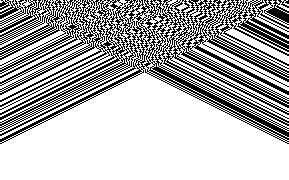
Figure 4: Temporal evolution of a parity solution of size 289, with convergence time 144. This image is obtained from a solution in $CT_{289}$ which is constructed as a single chain of cliques, and to flatten its graphical representation into a line. Each line in the image represents a configuration of the network, where white means $1$ and black means $0$. Time goes down.

Our second result is that any deciding Boolean network that is negation invariant provides a simple solution to the synchronisation problem. A network is negation invariant if $\neg F(x)=F(\neg x)$, for all $x\in\mathbb{B}^{n}$. Notice that both of these conditions are always true in the case of a parity solution built on the XOR function.

3.3 Solution to $k$-synchronisation

Theorem 3.2

If $F$ is a deciding automata network such that $\neg F(x)=F(\neg x)$, then $F^{\prime}=\neg\circ F$ is a solution to the synchronisation problem.

Proof

Since $\neg F(x)=F(\neg x)$, we have that

$F^{\prime}(F^{\prime}(x))=\neg F(\neg F(x))=\neg\neg F(F(x))=F(F(x))$.

As $F$ decides, $F\circ F$ also decides, which means that $F^{\prime}\circ F^{\prime}$ decides, which means that it always converges. Note that on $0^{n}$ or $1^{n}$, $F^{\prime}$ is simply the negation, and thus it synchronises. ∎

This theorem allows us to adapt our previous $CT$ solution to the synchronisation problem simply by taking any $F\in CT$ and adding a negation on all local functions, providing solutions for any odd value of $n$. Solutions for even $n$ can easily be provided by adding an extra automaton that takes the negation of any other automaton, at the price of breaking the strong connectivity of the network. The temporal evolution of a solution of size 289 is illustrated in Figure 5.

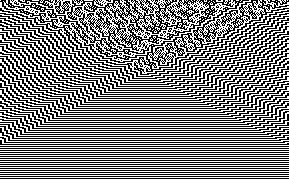
Figure 5: Temporal evolution of a synchronisation solution of size 289, with convergence time 144.

4 Generalisation to arbitrary alphabet sizes

We now prove that our construction generalises well to any finite alphabet $\Sigma$. Let $k=|\Sigma|$, we call $CT^{k}$ the families of solution that solve the $k$-parity problem. This generalisation rests on the fact that the XOR function is also the sum modulo $2$; for an alphabet of size $k$, we will instead use the sum modulo $k$ as the local function. Where we added $2$ automata for each new step of the construction of $CT^{2}_{n+2}$, in general we will add $k$ automata in the construction of $CT^{k}_{n+k}$, while $CT^{k}_{1}$ stays the identity network of size $1$ for all $k$. The interaction graph of a such a solution over the ternary alphabet is illustrated in Figure 6.

Figure 6: Interaction digraph of a solution in $CT^{3}_{16}$. Each local function is the sum modulo 3 of its influencing neighbours. The automata are numbered in one of the possible orders of addition that construct this solution.

In this generalisation, deciding means always converging to any fixed point $s^{n}$ for some $s\in\Sigma$. The generalisation of the parity problem is now the $k$-parity problem; to solve it, a network with alphabet $\Sigma$ must always converge to the fixed point with symbol the sum modulo $k$ of the values of the initial configuration.

The generalisation of the synchronisation problem is the $k$-synchronisation problem, where instead of oscillating between $0^{n}$ and $1^{n}$, a $k$-synchronising network over an alphabet of size $k$ must cycle through the $k$ previously described fixed points. While our construction cycles through these fixed points in increasing order, the order of this cycle is unimportant, as a solution with a different order can always be converted to a solution in any order.

Theorem 4.1

All $F\in CT^{k}$ solve the $k$-parity problem, i.e., the sum modulo $k$ decision problem.

Proof

This proof follows the same arguments as the binary case; given $x$ a starting configuration, initially every automaton computes the sum modulo $k$ of its neighbourhood of radius $0$.

Let us suppose that for values up to some $r$, all automata compute the sum modulo $k$ of the initial configuration over their neighbourhood of radius $r$ after $r$ steps. By the construction of the interaction digraph, the next update of all automata will result in a sum modulo $k$ of the value in the initial configuration of their neighbours of distance up to $r+1$, each neighbour being counted $m\times k+1$ times, for $m$ some positive integer.

As a result, after $r$ steps, every automaton computes the sum modulo $k$ of the values in the initial configuration of their neighbourhood of radius $r$. After $r=n$ steps, the network has solved the $k$-parity problem.

The temporal evolution of a solution to the 3-parity problem over a configuration of size 289 is illustrated in Figure 7.

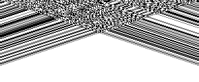
Figure 7: Temporal evolution of a 3-parity solution of size 289, with convergence time 96, flowing downwards. White means $2$, gray means $1$ and black means $0$.

Similarly, our argument that transformed the parity solution into a synchronisation solution also works for any finite alphabet; but instead of the invariance to be over the negation, we now require it to be over the $+1$ operator.

Theorem 4.2

If $F$ decides and is $+1$ invariant, then $F^{\prime}=(+1)\circ F$ is a solution to the $k$-synchronisation problem.

Proof

This proof follows the same arguments as the binary case: the $k$ repetition of $F^{\prime}$ is equivalent to the $k$ repetition of $F$ thanks to the invariance hypothesis. This means that since $F$ converges, $F^{k}$ also converges, and so $F^{\prime k}$ converges to a uniform configuration; this also implies that $F^{\prime}$ always converges to the cycles that go through every uniform fixed point in increasing order.

The temporal evolution of a synchronisation solution over the ternary alphabet and a configuration of size 289 is illustrated in Figure 8.

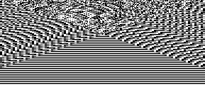
Figure 8: Temporal evolution of a 3-synchronisation solution of size 289, with convergence time 96, flowing downwards. White means $2$, gray means $1$ and black means $0$.

Whereas our the binary solution can be described as a collection fully connected cliques of size $3$ lightly connected to each other, the $k$-parity solution can be described as a collection of fully connected cliques of size $k+1$ lightly connected to each other.

5 Convergence times

5.1 Direct convergence

As a final analysis point, we present some facts about the convergence times of the presented solutions.

Central to the convergence proof is the fact that each automaton computes the sum modulo $k$ of its neighbourhood of radius $r$ after $r$ steps; this means that every automaton will have converged as soon as $r$ is large enough to include the entire graph. This value is exactly the diameter of the graph.

The interaction digraph of any solution in $CT^{k}$ could be described as a collection of cliques of size $k+1$ connected to each other through their nodes such as they form a tree; for any $n$ and $k$, the solution in $CT^{k}_{n}$ with the maximal diameter is the solution composed of cliques that together form a line. Let us call $C$ the number of such components and $D$ the diameter. In the case of a line, the diameter is always the number of cliques: $D=C$. Every connected component is of size $k+1$. By construction every connected component shares a node with the next, except for the last one; this means that overall, the network has $n=(C-1)\times k+(k+1)$ automata. We can infer the following:

$$n =(C-1)\times k+(k+1)=$$

$$=(D-1)\times k+k+1=$$

$$=D\times k+1,$$

which implies that $D=\frac{n-1}{k}$. In the binary case this means that the convergence times tends to $\frac{n}{2}$ as $n$ grows larger. Notice also that the convergence time decreases as $k$ grows larger for a given $n$; this is explained by the fact that a larger $k$ implies larger cliques which means that the network is more connected and has a smaller diameter relative to its size. This fact can be exploited to increase convergence time for a given $k$.

5.2 Trading component size for convergence time

For a given $k$, we can decrease convergence time as close to $0$ as desired by first constructing a solution for an alphabet of size a multiple of $k$, and then projecting that solution unto the alphabet of size $k$. By construction, this solution will converge faster, and it can be checked that it stills solves the sum modulo $k$ problem. For $m\in\mathbb{N}$, we denote $\pi_{mk,k}:\{0,\ldots,mk-1\}\to\{0,\ldots,k-1\}$ the projection which maps any $v$ to the reminder of the Euclidean division of $v$ by $k$.

Theorem 5.1

If $F\in CT^{mk}$, then $\pi_{mk,k}\circ F\in CT^{k}$.

Proof

Since after $r$ steps every automaton in $F$ computes the sum modulo $mk$ of its neighbourhood of radius $r$, it also follows that every automaton in $\pi_{mk,k}\circ F$ computes the sum modulo $k$ of its neighbourhood of radius $r$ in the same time.

The temporal evolution of a solution to the parity problem that converges twice as fast compared to the base solution is illustrated in Figure 9.

Hence for a given network with $n$ automata we can cut the convergence time of the network by a factor of $m$ by simply considering the solution for the alphabet of size $mk$, and projecting down. The trade-off of this acceleration is that this new solution needs to be constructed out of cliques of size $mk+1$, which means that each automaton has at least $mk+1$ neighbours. In other terms, the number of edges in the interaction graph grows as a polynomial of $k$.

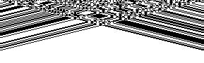
Figure 9: Temporal evolution of a faster parity solution of size 289, with convergence time 72, flowing downwards. This solution is the combination of the solution $CT^{4}_{289}$ together with a projection to the binary alphabet. It is guaranteed to converge twice as fast compared to any solution in $CT^{2}_{289}$.

This reasoning reaches its natural conclusion by simply taking $k=n-1$ and then projecting down, in which case the interaction digraph simply becomes the complete graph of size $n$, in which case computing the parity of the initial configuration only takes one step.

All of these observations also apply to our solutions to the $k$-synchronisation problem. The temporal evolution of such a solution in the binary synchronisation case projected down from the alphabet of size $4$ is illustrated in Figure 10.

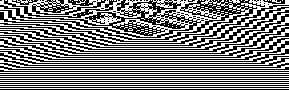
Figure 10: Temporal evolution of a faster synchronisation solution of size 289, with convergence time 72, flowing downwards. It has been obtained from a solution over the alphabet $\{0,1,2,3\}$ combined with a projection to the binary alphabet.

6 Concluding remarks

In this paper we presented solutions to the parity and synchronisation problems that are generalisable to any finite alphabet, using the flexible geometry of automata networks. The convergence time of these solutions is easy to compute and is always the diameter of their interaction graph. Further results are provided to accelerate this convergence time by projecting down a solution over an alphabet the size of which is a multiple of the desired solution’s alphabet.

Figures 4, 5, 7, 8, 9 and 10 all use configurations of size 289 specifically because 289 is one plus a multiple of $3$ and $4$, which allows these configurations to work in the context of their specific problem, while keeping a coherent pixel resolution throughout the illustrations of the paper.

The geometry of our solutions is more complex than the geometry of standard cellular automata lattices, yet they conserve a simple, local and repeatable form. We believe that this showcases interesting possibilities for designing new solutions to convergence problems in the realm of cellular automata. We believe other problems such as the well-known density classification task [3] could be approached this way.

References

- [1] M.M. Aburas, Y.M. Ho, M.F. Ramli, and Z.H. Ash’aari. The simulation and prediction of spatio-temporal urban growth trends using cellular automata models: A review. International Journal of Applied Earth Observation and Geoinformation, 52:380–389, 2016.
- [2] G. Bernot, J. Guespin-Michel, J.-P. Comet, P. Amar, A. Zemirline, F. Delaplace, P. Ballet, and A. Richard. Modeling, observability and experiment, a case study. In Proceedings of the Dieppe Spring school on Modelling and simulation of biological processes in the context of genomics, pages 49–55, 2003.
- [3] P.P.B. de Oliveira. On density determination with cellular automata: Results, constructions and directions. Journal of Cellular Automata, 9, 2014.
- [4] A.G. Hoekstra, J. Kroc, and P.M.A. Sloot. Introduction to modeling of complex systems using cellular automata. In Simulating Complex Systems by Cellular Automata, pages 1–16. Springer, 2010.
- [5] S. A. Kauffman. Metabolic stability and epigenesis in randomly constructed genetic nets. J. Theor. Biol., 22:437–467, 1969.
- [6] K.M. Lee, H. Xu, and H.F. Chau. Parity problem with a cellular automaton solution. Physical Review E, 64(2):026702, 2001.
- [7] C.L.M. Martins and P.P.B. de Oliveira. Improvement of a result on sequencing elementary cellular automata rules for solving the parity problem. Electronic Notes in Theoretical Computer Science, 252:103–119, 2009.
- [8] C.L.M. Martins and P.P.B. de Oliveira. Merging cellular automata rules to optimise a solution to the modulo-N problem. In Cellular Automata and Discrete Complex Systems: 21st IFIP WG 1.5 International Workshop, AUTOMATA 2015, Turku, Finland, June 8-10, 2015. Proceedings 21, pages 196–209. Springer, 2015.
- [9] A.R. Mikler, S. Venkatachalam, and K. Abbas. Modeling infectious diseases using global stochastic cellular automata. Journal of Biological Systems, 13(04):421–439, 2005.
- [10] M. Minsky and S. Papert. An introduction to computational geometry. Cambridge tiass., HIT, 479(480):104, 1969.
- [11] M. Montalva-Medel, P.P.B. de Oliveira, and E. Goles. A portfolio of classification problems by one-dimensional cellular automata, over cyclic binary configurations and parallel update. Natural Computing, 17:663–671, 2018.
- [12] S. Ninagawa. Solving the parity problem with elementary cellular automaton rule 60. Proc. of AUTOMATA and JAC, 2012, 2012.
- [13] E.L.P. Ruivo and P.P.B. de Oliveira. A perfect solution to the parity problem with elementary cellular automaton 150 under asynchronous update. Information Sciences, 493:138–151, 2019.
- [14] M. Sipper. Computing with cellular automata: Three cases for nonuniformity. Physical Review E, 57(3):3589, 1998.
- [15] R. Thomas. Boolean formalization of genetic control circuits. J. Theor. Biol., 42:563–585, 1973.
- [16] D.A. Wolf-Gladrow. Lattice-gas cellular automata and lattice Boltzmann models: an introduction. Springer, 2004.
- [17] D. Wolz and P.P.B. de Oliveira. Very effective evolutionary techniques for searching cellular automata rule spaces. Journal of Cellular Automata, 3(4), 2008.
- [18] H. Xu, K.M. Lee, and H.F. Chau. Modulo three problem with a cellular automaton solution. International Journal of Modern Physics C, 14(03):249–256, 2003.