4D Gaussian Splatting:
Towards Efficient Novel View Synthesis for Dynamic Scenes

Yuanxing Duan1*   Fangyin Wei2*   Qiyu Dai1,4   Yuhang He1   Wenzheng Chen3†   Baoquan Chen1,4†
1Peking University 2Princeton University 3NVIDIA 4National Key Lab of General AI, China
Abstract

We consider the problem of novel view synthesis (NVS) for dynamic scenes. Recent neural approaches have accomplished exceptional NVS results for static 3D scenes, but extensions to 4D time-varying scenes remain non-trivial. Prior efforts often encode dynamics by learning a canonical space plus implicit or explicit deformation fields, which struggle in challenging scenarios like sudden movements or capturing high-fidelity renderings. In this paper, we introduce 4D Gaussian Splatting (4DGS), a novel method that represents dynamic scenes with anisotropic 4D $XYZT$ Gaussians, inspired by the success of 3D Gaussian Splatting in static scenes [26]. We model dynamics at each timestamp by temporally slicing the 4D Gaussians, which naturally compose dynamic 3D Gaussians and can be seamlessly projected into images. As an explicit spatial-temporal representation, 4DGS demonstrates powerful capabilities for modeling complicated dynamics and fine details—especially for scenes with abrupt motions. We further implement our temporal slicing and splatting techniques in a highly optimized CUDA acceleration framework, achieving real-time inference rendering speeds of up to 277 FPS on an RTX 3090 GPU and 583 FPS on an RTX 4090 GPU. Rigorous evaluations on scenes with diverse motions showcase the superior efficiency and effectiveness of 4DGS, which consistently outperforms existing methods both quantitatively and qualitatively.

\begin{overpic}[height=88.2037pt,width=119.24821pt]{fig/figteaser/whiteim.png} \put(-2.0,19.0){ \includegraphics[height=65.44142pt,width=78.04842pt]{fig/figteaser/results/gt-coffee.png} } \put(2.0,14.0){ \includegraphics[height=65.44142pt,width=78.04842pt]{fig/figteaser/results/gt-coffee.png} } \put(6.0,9.0){ \includegraphics[height=65.44142pt,width=78.04842pt]{fig/figteaser/results/gt-coffee.png} } \put(10.0,4.0){ \includegraphics[height=65.44142pt,width=78.04842pt]{fig/figteaser/results/gt-coffee.png} } \put(14.0,0.0){ \leavevmode\hbox to92.95pt{\vbox to65.77pt{\pgfpicture\makeatletter\hbox{\hskip-0.2pt\lower 0.2pt\hbox to0.0pt{\pgfsys@beginscope\pgfsys@invoke{ }\definecolor{pgfstrokecolor}{rgb}{0,0,0}\pgfsys@color@rgb@stroke{0}{0}{0}\pgfsys@invoke{ }\pgfsys@color@rgb@fill{0}{0}{0}\pgfsys@invoke{ }\pgfsys@setlinewidth{0.4pt}\pgfsys@invoke{ }\nullfont\hbox to0.0pt{\pgfsys@beginscope\pgfsys@invoke{ }{{}}\hbox{\hbox{{\pgfsys@beginscope\pgfsys@invoke{ }{{}{}{{}}{} {{}{{}}}{{}{}}{}{{}{}} { }{{{{}}\pgfsys@beginscope\pgfsys@invoke{ }\pgfsys@transformcm{1.0}{0.0}{0.0}{1.0}{0.2pt}{0.2pt}\pgfsys@invoke{ }\hbox{{\definecolor{pgfstrokecolor}{rgb}{0,0,0}\pgfsys@color@rgb@stroke{0}{0}{0}\pgfsys@invoke{ }\pgfsys@color@rgb@fill{0}{0}{0}\pgfsys@invoke{ }\hbox{{\begin{overpic}[height=65.44142pt,width=89.43048pt]{fig/figteaser/results/gt-coffee.png}\put(66.6,66.6){\framebox{\leavevmode\hbox{\set@color\resizebox{}{}{{\leavevmode\hbox{\set@color{\includegraphics[width=24.28261pt,trim=1.00374pt 1.00374pt 1.00374pt 1.00374pt,clip]{fig/figteaser/results/3-cropped-gt-coffee.png}}}}}}}} \put(-25.4,66.6){\framebox{\leavevmode\hbox{\set@color\resizebox{}{}{{\leavevmode\hbox{\set@color{\includegraphics[width=23.84592pt,trim=2.00749pt 2.00749pt 2.00749pt 2.00749pt,clip]{fig/figteaser/results/4-cropped-gt-coffee.png}}}}}}}} \end{overpic} }} }}\pgfsys@invoke{\lxSVG@closescope }\pgfsys@endscope}}} \pgfsys@invoke{\lxSVG@closescope }\pgfsys@endscope}}} \pgfsys@beginscope\pgfsys@invoke{ }{ {}}{}{ {}}{} {}{{}}{} {}{{}}{}{}{}{}{{}}{}\pgfsys@beginscope\pgfsys@invoke{ }\color[rgb]{0.61,0.87,1.0}\definecolor[named]{pgfstrokecolor}{rgb}{0.61,0.87,1.0}\pgfsys@color@rgb@stroke{0.61}{0.87}{1.0}\pgfsys@invoke{ }\pgfsys@color@rgb@fill{0.61}{0.87}{1.0}\pgfsys@invoke{ }\definecolor[named]{pgffillcolor}{rgb}{0.61,0.87,1.0}\pgfsys@setlinewidth{0.6pt}\pgfsys@invoke{ }{}\pgfsys@moveto{40.79279pt}{12.24048pt}\pgfsys@moveto{40.79279pt}{12.24048pt}\pgfsys@lineto{40.79279pt}{18.85745pt}\pgfsys@lineto{47.60703pt}{18.85745pt}\pgfsys@lineto{47.60703pt}{12.24048pt}\pgfsys@closepath\pgfsys@moveto{47.60703pt}{18.85745pt}\pgfsys@stroke\pgfsys@invoke{ } \pgfsys@invoke{\lxSVG@closescope }\pgfsys@endscope{}{{}}{} {}{{}}{}{}{}{}{{}}{}\pgfsys@beginscope\pgfsys@invoke{ }\color[rgb]{1.0,0.74,0.85}\definecolor[named]{pgfstrokecolor}{rgb}{1.0,0.74,0.85}\pgfsys@color@rgb@stroke{1.0}{0.74}{0.85}\pgfsys@invoke{ }\pgfsys@color@rgb@fill{1.0}{0.74}{0.85}\pgfsys@invoke{ }\definecolor[named]{pgffillcolor}{rgb}{1.0,0.74,0.85}\pgfsys@setlinewidth{0.6pt}\pgfsys@invoke{ }{}\pgfsys@moveto{71.50525pt}{5.09448pt}\pgfsys@moveto{71.50525pt}{5.09448pt}\pgfsys@lineto{71.50525pt}{9.79218pt}\pgfsys@lineto{76.35811pt}{9.79218pt}\pgfsys@lineto{76.35811pt}{5.09448pt}\pgfsys@closepath\pgfsys@moveto{76.35811pt}{9.79218pt}\pgfsys@stroke\pgfsys@invoke{ } \pgfsys@invoke{\lxSVG@closescope }\pgfsys@endscope \pgfsys@invoke{\lxSVG@closescope }\pgfsys@endscope \pgfsys@invoke{\lxSVG@closescope }\pgfsys@endscope{}{}{}\hss}\pgfsys@discardpath\pgfsys@invoke{\lxSVG@closescope }\pgfsys@endscope\hss}}\lxSVG@closescope\endpgfpicture}} } \end{overpic} \begin{overpic}[height=88.2037pt,width=119.24821pt]{fig/figteaser/results/ours-coffee.png}\put(75.0,50.0){\framebox{\leavevmode\hbox{\set@color\resizebox{}{}{{\leavevmode\hbox{\set@color{\includegraphics[width=24.28261pt,trim=1.00374pt 1.00374pt 1.00374pt 1.00374pt,clip]{fig/figteaser/results/3-cropped-ours-coffee.png}}}}}}}} \put(0.0,50.0){\framebox{\leavevmode\hbox{\set@color\resizebox{}{}{{\leavevmode\hbox{\set@color{\includegraphics[width=23.84592pt,trim=2.00749pt 2.00749pt 2.00749pt 2.00749pt,clip]{fig/figteaser/results/4-cropped-ours-coffee.png}}}}}}}} \end{overpic} \begin{overpic}[height=88.2037pt,width=119.24821pt]{fig/figteaser/results/hyperreel-coffee.png}\put(75.0,50.0){\framebox{\leavevmode\hbox{\set@color\resizebox{}{}{{\leavevmode\hbox{\set@color{\includegraphics[width=24.28261pt,trim=1.00374pt 1.00374pt 1.00374pt 1.00374pt,clip]{fig/figteaser/results/3-cropped-hyperreel-coffee.png}}}}}}}} \put(0.0,50.0){\framebox{\leavevmode\hbox{\set@color\resizebox{}{}{{\leavevmode\hbox{\set@color{\includegraphics[width=23.84592pt,trim=2.00749pt 2.00749pt 2.00749pt 2.00749pt,clip]{fig/figteaser/results/4-cropped-hyperreel-coffee.png}}}}}}}} \end{overpic} [Uncaptioned image]
Dynamic Video Input The Proposed Method HyperReel [2] Evaluation on PSNR vs. FPS
Figure 1: We present 4D Gaussian Splatting, a novel approach that takes videos as input and synthesizes dynamic novel-view images with fine details. The proposed method outperforms prior arts in rendering quality and achieves up to 277 FPS inference speed on an RTX 3090 GPU at Plenoptic Dataset [33].
footnotetext: * Equal contributionfootnotetext: $\dagger$ Co-corresponding authors

1 Introduction

Reconstructing 3D scenes from 2D images and synthesizing their appearance from novel views has been a long-standing goal in computer vision and graphics. This task is pivotal in numerous industrial applications including film, gaming, and VR/AR, where there is a substantial demand for high-speed, photo-realistic rendering effects. The task diverges into two different scene types: static scenes where objects are still across all images [37, 27, 24, 4] and dynamic scenes where scene contents exhibit temporal variations [43, 40, 33, 57, 11]. While the former has witnessed significant progress recently, efficient and accurate NVS for dynamic scenes remains challenging due to the complexities introduced by the temporal dimension and diverse motion patterns.

A variety of methods have been proposed to tackle the challenges posed by dynamic NVS. A series of methods model the 3D scene and its dynamics jointly [14, 21]. However, these methods often fall short in preserving fine details in the NVS renderings due to the complexity caused by the highly entangled spatial and temporal dimensions. Alternatively, many existing techniques [39, 40, 51, 43, 15] decouple dynamic scenes by learning a static canonical space and then predicting a deformation field to account for the temporal variations. Nonetheless, this paradigm struggles in capturing complex dynamics such as objects appearing or disappearing suddenly. More importantly, prevailing methods on dynamic NVS mostly build upon volumetric rendering [37] which requires dense sampling on millions of rays. As a consequence, these methods typically cannot support real-time rendering speed even for static scenes [33, 47].

Recently, 3D Gaussian Splatting (3DGS) [26] has emerged as a powerful tool for efficient NVS of static scenes. By explicitly modeling the scene with 3D Gaussian ellipsoids and employing fast rasterization technique, it achieves photo-realistic NVS in real time. Inspired by this, we propose to lift Gaussians from 3D to 4D and provide a novel spatial-temporal representation that enables NVS for more challenging dynamic scenes.

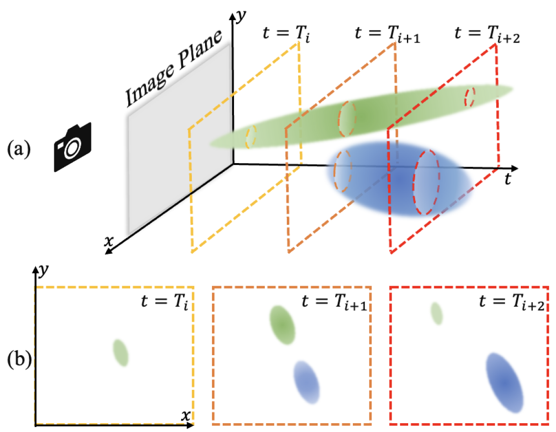
Our key observation is that 3D scene dynamics at each timestamp can be viewed as 4D spatial-temporal Gaussian ellipsoids sliced with different time queries. Fig. 2 illustrates a simplified $XYT$ case: the dynamics in 2D $XY$ space at time $T_{i}$ is equivalent to building 3D $XYT$ Gaussians and slicing by the $t=T_{i}$ plane. Analogously, we extend 3D Gaussians to 4D $XYZT$ space to model dynamic 3D scenes. The temporally sliced 4D Gaussians compose 3D Gaussians that can be seamlessly projected to 2D screens via fast rasterization, inheriting both exquisite rendering effects and high speed characteristic from 3DGS. Moreover, extending the prune-split mechanism in the temporal dimension makes 4D Gaussians particularly suitable for representing complex dynamics, including abrupt appearances or disappearances.

It is non-trivial to lift 3D Gaussians into 4D space, where tremendous challenges exist in the design of the 4D rotation, slicing, as well as the joint spatial-temporal optimization scheme. We draw inspiration from geometric algebra and carefully choose 4D rotor [6] to represent 4D rotation, which is a spatial-temporal separable rotation representation. Notably, rotor representation accommodates both 3D and 4D rotation: when the temporal dimension is set to zero, it becomes equivalent to a quaternion and can represent 3D spatial rotation as well. Such adaptability grants our method the flexibility to model both dynamic and static scenes. In other words, 4DGS is a generalizable form of 3DGS: when closing the temporal dimension, our 4DGS reduces to 3DGS.

We enhance the optimization strategies in 3DGS and introduce two new regularization terms to stabilize and improve the dynamic reconstruction. We first propose an entropy loss that pushes the opacity of Gaussians towards either one or zero, which proves effective to remove “floaters” in our experiments. We further introduce a novel 4D consistency loss to regularize the motion of Gaussian points and yield more consistent dynamics reconstruction. Experiments show that both terms notably improve the rendering quality.

While existing Gaussian-based methods [35, 60, 56, 61] are mostly based on PyTorch [41], we further develop a highly optimized CUDA framework with careful engineering designs for fast training and inference speed. Our framework supports rendering 1352$\times$1014 videos at an unprecedented 583 FPS on an RTX 4090 GPU and 277 FPS on an RTX 3090 GPU. We conduct extensive experiments on two datasets spanning a wide range of settings and motion patterns, including monocular videos [43] and multi-camera videos [33]. Quantitative and qualitative evaluations demonstrate the distinct advantages over preceding methods, including the new state-of-the-art rendering quality and speed.

2 Related Work

Refer to caption
Figure 2: A Simplified 2D Illustration of the Proposed Temporal Slicing. (a) we model 2D dynamics with 3D $XYT$ ellipsoids and slice them with different time queries. (b) The sliced 3D ellipsoids form 2D dynamic ellipses at each timestamp.

In this section, we mainly review optimization-based novel view synthesis (NVS) methods, where the input is a set of posed images and the output is new appearance from novel viewpoints. We first describe NVS for static scenes, then talk about its dynamic extensions. Lastly, we discuss recent Gaussian-based NVS methods.

Static Novel View Synthesis Previous approaches formalize light-field [30] or lumigraph [22, 7] that generate novel-view images by interpolating from existing views, which require densely captured images in order to acquire realistic renderings. Other classical methods exploit geometric proxies such as mesh and volume to reproject and blend contents from source images onto novel views. Mesh-based methods [13, 44, 49, 53, 55] represent the scenes with surfaces that support efficient rendering but are hard to optimize. Volume-based methods use voxel grids [29, 42, 45] or multi-plane images (MPIs) [17, 36, 48, 63], which provide delicate rendering effects but are memory-inefficient or limited to small view changes. Recently, the trend of NVS was spearheaded by Neural Radiance Fields (NeRFs) [37], which achieves photo-realistic rendering quality. Since then, a series of efforts have emerged to improve the training speed [38, 18, 10], enhance rendering quality [3, 52], or extend to more challenging scenarios such as reflection and refraction [28, 5, 59]. Still, most of these methods rely on volume rendering that requires sampling millions of rays and hinders real-time rendering [37, 3, 10].

Dynamic Novel View Synthesis This poses new challenges due to the temporal variations in the input images. Traditional methods estimate varying geometries such as surfaces [31, 12] and depth maps [25, 64] to account for dynamics. Inspired by NeRFs, recent work typically models dynamic scenes with neural representations. A branch of methods implicitly model the dynamics by adding a temporal input or latent code [14, 21]. Another line of works [39, 40, 51, 43, 15] explicitly model deformation fields that map 3D points at arbitrary timestamp into a canonical space. Other techniques explore decomposing a scene into static and dynamic components [47], using key frames to reduce redundancy [33, 2], estimating a flow field [34, 23, 50], or exploiting 4D grid-based representations [32, 19, 8, 54, 15, 20, 46]etc. The common issues of dynamic scene modeling are the complexities introduced by the spatial-temporal entanglement, as well as the additional memory and time cost caused by the temporal dimension.

Gaussian-Based NVS The recent seminal work [62, 58, 1, 26] models static scenes with Gaussians whose positions and appearance are learned through a differentiable splatting-based renderer. Particularly, 3D Gaussian Splatting (3DGS) [26] achieves impressive real-time rendering thanks to its Gaussian split/clone operations and the fast splatting-based rendering technique. Our work draws inspiration from 3DGS but lifts 3D Gaussians into 4D space and focuses on dynamic scenes. Several concurrent works also extend 3DGS to model dynamics. Deformable3DGS [35] directly learns the temporal motion and rotation of each 3D Gaussian along time, which makes it suitable for dynamic tracking applications. Similarly, [60, 56] utilize MLPs to predict the temporal movement. However, it is challenging for these methods to represent dynamic contents that suddenly appear or disappear. Similar to us, RealTime4DGS [61] also leverages 4D Gaussian representation to model 3D dynamics. They choose a dual-quaternion based 4D rotation formulation that is less interpretable and lacks the spatial-temporal separable property compared to rotor-base representation. Moreover, we further investigate better spatial-temporal optimization strategies and develop a high-performance framework that achieves much higher rendering speed and better rendering quality.
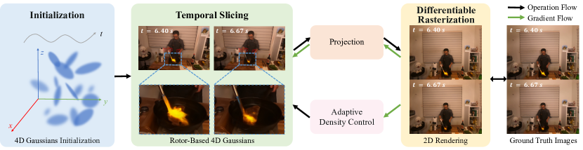
3 Method

In this section, we first review the 3D Gaussian Splatting (3DGS) method [26] in Sec. 3.1. We then describe our 4G Gaussian Splatting algorithm in Sec. 3.2, where we present rotor-based 4D Gaussian representation in Sec. 3.2.1 and discuss the temporal slicing technique for differentiable real-time rasterization in Sec. 3.2.2. Finally, we introduce our dynamic optimization strategies in Sec. 3.3.

3.1 Preliminary of 3D Gaussian Splatting

3D Gaussian Splatting (3DGS) [26] has demonstrated real-time, state-of-the-art rendering quality on static scenes. It models a scene with a dense cluster of $N$ anisotropic 3D Gaussian ellipsoids. Each Gaussian is represented by a full 3D covariance matrix $\mathbf{\Sigma}$ and its center position $\mathbf{\mu}$:

$${G}(\mathbf{x})=e^{-\frac{1}{2}(\mathbf{x}-\mathbf{\mu})^{T}\mathbf{\Sigma}^{-1}(\mathbf{x}-\mathbf{\mu})}.$$ (1)

To ensure a valid positive semi-definite covariance matrix during optimization, $\mathbf{\Sigma}$ is decomposed into the scaling matrix $\mathbf{S}$ and the rotation matrix $\mathbf{R}$ to characterize the geometry of a 3D Gaussian ellipsoid:

$$\mathbf{\Sigma}=\mathbf{R}\mathbf{S}\mathbf{S}^{T}\mathbf{R}^{T},$$ (2)

where $\mathbf{S}=\text{diag}(s_{x},s_{y},s_{z})\in\mathbb{R}^{3}$ and $\mathbf{R}\in SO(3)$ are stored as a $3D$ vector and quaternion, respectively. Beyond $\mathbf{\mu}$, $\mathbf{S}$ and $\mathbf{R}$, each Gaussian maintains additional learnable parameters including opacity $o\in(0,1)$ and spherical harmonic (SH) coefficients in $\mathbb{R}^{k}$ representing view-dependent colors ($k$ is related to SH order). During optimization, 3DGS adaptively controls the Gaussian distribution by splitting and cloning Gaussians in regions with large view-space positional gradients, as well as the culling of Gaussians that exhibit near-transparency.

Efficient rendering and parameter optimization in 3DGS are powered by the differentiable tile-based rasterizer. Firstly, 3D Gaussians are projected to 2D space by computing the camera space covariance matrix $\mathbf{\Sigma^{\prime}}$:

$$\mathbf{\Sigma^{\prime}}=\mathbf{J}\mathbf{V}\mathbf{\Sigma}\mathbf{V}^{T}\mathbf{J}^{T},$$ (3)

where $\mathbf{J}$ is the Jacobian matrix of the affine approximation of the projection transformation, and $\mathbf{V}$ is the extrinsic camera matrix. Then, the color of each pixel on the image plane is calculated by blending Gaussians sorted by their depths:

$$C=\sum_{i=1}^{N}c_{i}\alpha_{i}\prod_{j=1}^{i-1}(1-\alpha_{j}),$$ (4)

where $c_{i}$ is the color of the $i$-th 3D Gaussian ${G}_{i}$, $\alpha_{i}=o_{i}G^{\prime}_{i}$ with $o_{i}$ and $G^{\prime}_{i}$ as the opacity and 2D projection of ${G}_{i}$, respectively. Please refer to 3DGS [26] for more details.

3.2 4D Gaussian Splatting

We now discuss our 4D Gaussian Splatting (4DGS) algorithm. Specifically, we model the 4D Gaussian with rotor-based rotation representation (Sec. 3.2.1) and slice the time dimension to generate dynamic 3D Gaussians at each timestamp (Sec. 3.2.2). The 3D Gaussian ellipsoids sliced at each timestamp can be efficiently rasterized onto a 2D image plane for real-time and high-fidelity rendering of dynamic scenes.

Refer to caption
Figure 3: Framework Overview. After initialization, we first temporally slice the 4D Gaussians whose spatio-temporal movements are modeled with rotors. The dynamics such as the flickering flames naturally evolve through time, even within a short period of less than 0.3 second. The sliced 3D Gaussians are then projected onto 2D using differentiable rasterization. The gradients from image difference loss are back-propagated and guide the adaptive density control of 4D Gaussians.

3.2.1 Rotor-Based 4D Gaussian Representation

Analogous to 3D Gaussians, a 4D Gaussian can be expressed with the 4D center position $\mathbf{\mu}_{4D}=(\mathbf{\mu}_{x},\mathbf{\mu}_{y},\mathbf{\mu}_{z},\mathbf{\mu}_{t})$ and the 4D covariance matrix $\mathbf{\Sigma}_{4D}$ as

$${G}_{4D}(x)=e^{-\frac{1}{2}(x-\mathbf{\mu}_{4D})^{T}\mathbf{\Sigma}_{4D}^{-1}(x-\mathbf{\mu}_{4D})}.$$ (5)

The covariance $\Sigma_{4D}$ can be further factorized into the 4D scaling $S_{4D}$ and the 4D rotation $R_{4D}$ as

$$\mathbf{\Sigma}_{4D}=\mathbf{R}_{4D}\mathbf{S}_{4D}\mathbf{S}_{4D}^{T}\mathbf{R}_{4D}^{T}.$$ (6)

While modeling $\mathbf{S}_{4D}=\text{diag}(s_{x},s_{y},s_{z},s_{t})$ is straightforward, seeking a proper 4D rotation representation for $R_{4D}$ is a challenging problem.

In geometric algebra, rotations of high-dimensional vectors can be described using rotors [6]. Motivated by this, we introduce 4D rotors to characterize the 4D rotations. A 4D rotor $\mathbf{r}$ is composed of 8 components based on a set of basis:

$\displaystyle\mathbf{r}$ $\displaystyle=s+b_{01}\mathbf{e}_{01}+b_{02}\mathbf{e}_{02}+b_{03}\mathbf{e}_{03}+b_{12}\mathbf{e}_{12}$
$\displaystyle\quad+b_{13}\mathbf{e}_{13}+b_{23}\mathbf{e}_{23}+p\mathbf{e}_{0123},$ (7)

where $\mathbf{e}_{0123}=\mathbf{e}_{0}\wedge\mathbf{e}_{1}\wedge\mathbf{e}_{2}\wedge\mathbf{e}_{3}$, and $\mathbf{e}_{ij}=\mathbf{e}_{i}\wedge\mathbf{e}_{j}$ is the outer product between 4D axis $\mathbf{e}_{i}$ ($i\in\{0,1,2,3\}$) that form the orthonormal basis in 4D Euclidean space. Therefore, a 4D rotation can be determined by 8 coefficients $\left(s,b_{01},b_{02},b_{03},b_{12},b_{13},b_{23},p\right)$.

Analogous to quaternion, a rotor $\mathbf{r}$ can also be converted into a 4D rotation matrix $\mathbf{R}_{4D}$ with proper normalization function $\mathcal{F}_{norm}$ and rotor-matrix mapping function $\mathcal{F}_{map}$. We carefully derive a numerically stable normalization method for rotor transformation and provide details of the two functions in Supplementary Material:

$$\mathbf{R}_{4D}=\mathcal{F}_{map}(\mathcal{F}_{norm}(\mathbf{r})).$$ (8)

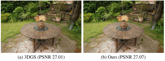
Our rotor-based 4D Gaussian offers a well-defined, interpretable rotation representation: the first four components encode the 3D spatial rotation, and the last four components define spatio-temporal rotation, i.e., spatial translation. In particular, setting the last four components to zero effectively reduces $\mathbf{r}$ to a quaternion for 3D spatial rotation, thereby enabling our framework to model both static and dynamic scenes. Fig. 4 presents an example where our result on a static 3D scene matches that of original 3DGS [26].

Alternatively, concurrent work [61] also models dynamic scenes with 4D Gaussian. However, they represent 4D rotation with two entangled isoclinic quaternions [9]. As a result, their spatial and temporal rotations are tightly coupled, and it is unclear how to constrain and normalize this alternative rotation representation during optimization to model static 3D scenes.

3.2.2 Temporally-Sliced 4D Gaussians Splatting

We now describe how to slice 4D Gaussians into 3D space. Given that $\mathbf{\Sigma}_{4D}$ and its inverse $\mathbf{\Sigma}_{4D}^{-1}$ are both symmetric matrices, we define

$$\mathbf{\Sigma}_{4D}=\left(\begin{matrix}\mathbf{U}&\mathbf{V}\\ \mathbf{V}^{T}&\mathbf{W}\\ \end{matrix}\right)\text{~{}and~{}}\mathbf{\Sigma}_{4D}^{-1}=\left(\begin{matrix}\mathbf{A}&\mathbf{M}\\ \mathbf{M}^{T}&\mathbf{Z}\\ \end{matrix}\right),$$ (9)

where both $\mathbf{U}$ and $\mathbf{A}$ are $3\times 3$ matrices. Then, given a time $t$, the projected 3D Gaussian is obtained as (detailed derivation in the Supplementary Material):

$${G}_{3D}(\mathbf{x},t)=\text{e}^{-\frac{1}{2}\lambda(t-\mathbf{\mu}_{t})^{2}}\text{e}^{-\frac{1}{2}\left[\mathbf{x}-\mathbf{\mu}(t)\right]^{T}\mathbf{\Sigma}_{3D}^{-1}\left[\mathbf{x}-\mathbf{\mu}(t)\right]},$$ (10)

where

$\displaystyle\lambda$ $\displaystyle=\mathbf{W}^{-1},$ (11)
$\displaystyle\mathbf{\Sigma}_{3D}$ $\displaystyle=\mathbf{A}^{-1}=\mathbf{U}-\dfrac{\mathbf{V}\mathbf{V}^{T}}{\mathbf{W}},$
$\displaystyle\mathbf{\mu}(t)$ $\displaystyle=(\mathbf{\mu}_{x},\mathbf{\mu}_{y},\mathbf{\mu}_{z})^{T}+(t-\mathbf{\mu}_{t})\dfrac{\mathbf{V}}{\mathbf{W}}.$

Compared with Eq. 1 in the original 3DGS [26], the sliced 3D Gaussian in Eq. 10 contains a temporal decay term $\text{e}^{-\frac{1}{2}\lambda(t-\mathbf{\mu}_{t})^{2}}$. As $t$ goes by, a Gaussian point first appears once $t$ is sufficiently close to its temporal position $\mathbf{\mu}_{t}$ and starts to grow. It reaches the peak opacity when $t=\mathbf{\mu}_{t}$. After that, the 3D Gaussian gradually shrinks in density until vanishing when $t$ is sufficiently far from $\mathbf{\mu}_{t}$. By controlling the temporal position and scaling factor, 4D Gaussian can represent challenging dynamics, e.g., motions that suddenly appear or disappear. During rendering, we filter points that are too far from current time, where the threshold for visibility $\frac{1}{2}\lambda(t-\mathbf{\mu}_{t})^{2}$ is empirically set to 16.

Moreover, the sliced 3D Gaussian exhibits a new motion term of $(t-\mathbf{\mu}_{t}){\mathbf{V}}/{\mathbf{W}}$ added to the center position $(\mathbf{\mu}_{x},\mathbf{\mu}_{y},\mathbf{\mu}_{z})^{T}$. In theory, linear movement of a 3D Gaussian emerges from our 4D slicing operation. We assume in a small time interval, all motions can be approximated by linear motions, and more complex non-linear cases can be represented by combination of multiple Gaussians. Further, ${\mathbf{V}}/{\mathbf{W}}$ indicates the motion speed in the current timestamp. Therefore, by modeling a scene with our framework, we can acquire speed field for free. We visualize the optical flow in Fig. 8.

Finally, following 3DGS [26], we project the sliced 3D Gaussians to the 2D image plane in depth order and perform the fast differentiable rasterization to obtain the final image. We implement rotor representation and slicing in a high-performance CUDA framework and achieve much higher rendering speed compared to PyTorch implementation.

Refer to caption
Figure 4: Modeling 3D Static Scenes. Our rotor-based representation enables both 3D static and 4D dynamic scene modeling. Our framework matches the results of 3DGS [26] on static 3D scenes.

3.3 Optimization Schema

When lifting 3D Gaussians into 4D space, the increased dimension extends the freedom of Gaussian points. Therefore, we introduce two regularization terms to help stabilize the training process: entropy loss and 4D consistency loss.

3.3.1 Entropy Loss

Similar to NeRFs, each Gaussian point has a learnable opacity term $o_{i}$ and the volume rendering formula is applied to composite the final color. Ideally, a Gaussian point should be close to the object surface, and in most cases its opacity should be close to one. Therefore, we encourage the opacity to be close to one or close to zero by adding an entropy loss, and by default Gaussians with near-zero opacity will be pruned during training:

$\displaystyle L_{\text{entropy}}=$ $\displaystyle\frac{1}{N}\sum_{i=1}^{N}-o_{i}log(o_{i}).$ (12)

We find that $L_{\text{entropy}}$ helps condense Gaussian points and filter noisy floaters, which is very useful when training with sparse views.

3.3.2 4D Consistency Loss

Intuitively, nearby Gaussians in 4D space should have similar motions. We further regularize the 4D Gaussian points by adding the 4D spatial-temporal consistency loss. Recall when slicing a 4D Gaussian at a given time $t$, a speed term $\mathbf{s}$ is derived. Thus, given the $i$-th Gaussian point, we gather $K$ nearest 4D points from its neighbour space $\Omega_{i}$ and regularize their motions to be consistent:

$\displaystyle L_{\text{consistent4D}}=$ $\displaystyle\frac{1}{N}\sum_{i=1}^{N}\left|\left|\mathbf{s}_{i}-\frac{1}{K}\sum_{j\in\Omega_{i}}\mathbf{s}_{j}\right|\right|_{1}.$ (13)

For 4D Gaussians, 4D distance is a better metric for point similarity than 3D distance, because points that are neighbors in 3D do not necessarily follow the same motions, e.g., when they belong to two objects with different motions. Note that calculating 4D nearest neighbors is uniquely and naturally enabled in our 4D representation, which cannot be exploited by deformation-based methods [56]. We balance the different scales of each dimension by dividing with the corresponding spacial and temporal scene scales.

3.3.3 Total Loss

We follow original 3DGS [26] and add $L_{1}$ and SSIM losses between the rendered images and ground truth images. Our final loss is defined as:

$\displaystyle L=$ $\displaystyle(1-\lambda_{1})L_{1}+\lambda_{1}L_{ssim}+\lambda_{2}L_{\text{entropy}}+\lambda_{3}L_{\text{consistent4D}}.$ (14)

3.3.4 Optimization Framework

We implement two versions of our method: one using PyTorch for fast development and one highly-optimized equivalent in C++ and CUDA for fast training and inference. Compared to the PyTorch version, our CUDA acceleration allows to render at an unprecedented 583 FPS at 1352$\times$1014 resolution on a single NVIDIA RTX 4090 GPU. Further, our CUDA framework also accelerates training by 16.6x. For benchmarking with baselines, we also test our framework on an RTX 3090 GPU and achieve 277 FPS, which significantly outperforms current state of the art (114 FPS [61]).

4 Experiments

4.1 Datasets

We evaluate our method on two commonly used datasets that are representative of various challenges in dynamic scene modeling. Plenoptic Video Dataset [33] contains real-world multi-view videos of 6 scenes. It includes abrupt motion as well as transparent and reflective materials. Following prior work [33], we use resolution of 1352$\times$1014. D-NeRF Dataset [43] contains one-second monocular videos for 8 synthetic scenes. We use resolution of 400$\times$400 following standard practice [43].

4.2 Implementation Details

Initialization. We uniformly sample 100,000 points in a 4D bounding box as Gaussian means. For Plenoptic dataset, we initialize with colored COLMAP [16] reconstruction. 3D scales are set as the distance to the nearest neighbor. Rotors are initialized with $(1,0,0,0,0,0,0,0)$ equivalent of static identity transformation.

Training. Using Adam optimizer, we train for 20,000 steps with batch size 3 on D-NeRF dataset and 30,000 steps with batch size 2 on Plenoptic dataset. Densification gradient thresholds are $5e-5$ and $2e-4$ for D-NeRF and Plenoptic datasets, respectively. We set $\lambda_{1}=0.2,\lambda_{2}=0.01,\lambda_{3}=0.05$, and $K=8$, except that $\lambda_{2}=0$ for Plenoptic dataset since its videos contain a large number of transparent objects. Learning rates, densification, pruning, and opacity reset settings all follow [26].

CUDA Acceleration. We implemented the forward and backward functions of 4D rotors to 4D rotation matrices and 4D Gaussian slicing in our customized CUDA training framework. The duplication and pruning of the 4D Gaussians are also performed by CUDA, ensuring a low GPU memory usage.

4.3 Baselines

We compare with both NeRF-based and concurrent Gaussian-based methods on the two datasets. Most compared methods have released official codebase, in which case we run the code as is and report the obtained numbers for novel view rendering quality, training time, and inference speed. Otherwise, we copy the results from their papers. All the numbers reported in the tables are benchmarked on an NVIDIA RTX 3090 GPU.

Refer to caption  Refer to caption  Refer to caption   Refer to caption  Refer to caption  Refer to caption   Refer to caption  Refer to caption  Refer to caption   Refer to caption  Refer to caption  Refer to caption   Refer to caption  Refer to caption  Refer to caption  
HyperReel MixVoxels RealTime4DGS Ours Ground Truth
Figure 5: Qualitative Comparison on Plenoptic Video Dataset. Compared with previous state of the arts, our method recovers finer details of dynamic regions, e.g., the magnified human face and hand. Our method also produces sharper rendering of static regions, e.g., the outdoor backgrounds around the human head in scene Flame Salmon and the zoomed-in hook in scene Cook Spinach.

4.4 Results

4.4.1 Evaluation on Plenoptic Video Dataset

As detailed in Tab. 1, prior work struggles with trade-offs between rendering speed and quality, due to the slow volume rendering (a-f), time cost of querying neural network components (c, d, g), or the spatial-temporal entanglement (a, c, g). Our method, however, exhibits significant advantages. Foremost, it markedly outperforms existing work in rendering high-resolution videos (1352$\times$1014) at 277 FPS on an NVIDIA RTX 3090 GPU, over 10x faster than NeRF-based methods (a-f) and over 2x faster than Gaussian-based methods (g, h). Moreover, our method achieves the highest PSNR of 31.62 (vs. the previous best 30.85) with a short average training time of 60 min.

As presented in Fig. 5, our method promotes a clearer and more detailed reconstruction of dynamic regions over baselines. For all four scenes, the proposed approach reconstructs higher-quality human heads that move frequently and contain high-frequency details. As magnified in the first three scenes, baselines may produce blurry artifacts for the hand regions with fast motions. In comparison, our method yields the sharpest renderings for the same regions.

Table 1: Evaluation on Plenoptic Video Dataset. We compare our method with both NeRF-based an Gaussian-based approaches. Our method significantly outperforms baselines on PSNR and inference speed. *:Only tested on the scene Flame Salmon. **:Trained on 8 GPUs. †: Results from paper.
ID Method PSNR$\uparrow$ SSIM$\uparrow$ LPIPS$\downarrow$ Train$\downarrow$ FPS$\uparrow$
a DyNeRF [33]*† 29.58 - 0.08 1344 h** 0.015
b StreamRF [32] 28.16 0.85 0.31 79 min 8.50
c HyperReel [2] 30.36 0.92 0.17 9 h 2.00
d NeRFPlayer [47] 30.69 - 0.11 6 h 0.05
e K-Planes [19] 30.73 0.93 0.07 190 min 0.10
f MixVoxels [54] 30.85 0.96 0.21 91 min 16.70
g Deformable4DGS [56] 28.42 0.92 0.17 72 min 39.93
h RealTime4DGS [61] 29.95 0.92 0.16 8 h 72.80
i Ours 31.62 0.94 0.14 60 min 277.47
Lego Jumping Jacks Stand Up T-Rex Hook

TiNeuVox

\begin{overpic}[width=82.38885pt]{fig/dnerf-main/tinuevox_lego-with_rect.png} \put(62.0,62.0){\framebox{\leavevmode\hbox{\set@color\resizebox{}{}{{\leavevmode\hbox{\set@color{\includegraphics[width=30.35657pt,trim=3.01125pt 3.01125pt 3.01125pt 3.01125pt,clip]{fig/dnerf-main/tinuevox_lego-cropped.png}}}}}}}} \end{overpic} \begin{overpic}[width=82.38885pt]{fig/dnerf-main/tinuevox_jumpingjacks-with_rect.png} \put(62.0,62.0){\framebox{\leavevmode\hbox{\set@color\resizebox{}{}{{\leavevmode\hbox{\set@color{\includegraphics[width=30.35657pt,trim=3.01125pt 3.01125pt 3.01125pt 3.01125pt,clip]{fig/dnerf-main/tinuevox_jumpingjacks-cropped.png}}}}}}}} \end{overpic} \begin{overpic}[width=82.38885pt]{fig/dnerf-main/tinuevox_standup-with_rect.png} \put(62.0,62.0){\framebox{\leavevmode\hbox{\set@color\resizebox{}{}{{\leavevmode\hbox{\set@color{\includegraphics[width=30.35657pt,trim=3.01125pt 3.01125pt 3.01125pt 3.01125pt,clip]{fig/dnerf-main/tinuevox_standup-cropped.png}}}}}}}} \end{overpic} \begin{overpic}[width=82.38885pt]{fig/dnerf-main/tinuevox_trex-with_rect.png} \put(62.0,62.0){\framebox{\leavevmode\hbox{\set@color\resizebox{}{}{{\leavevmode\hbox{\set@color{\includegraphics[width=30.35657pt,trim=3.01125pt 3.01125pt 3.01125pt 3.01125pt,clip]{fig/dnerf-main/tinuevox_trex-cropped.png}}}}}}}} \end{overpic} \begin{overpic}[width=82.38885pt]{fig/dnerf-main/tinuevox_hook-with_rect.png} \put(62.0,62.0){\framebox{\leavevmode\hbox{\set@color\resizebox{}{}{{\leavevmode\hbox{\set@color{\includegraphics[width=30.35657pt,trim=3.01125pt 3.01125pt 3.01125pt 3.01125pt,clip]{fig/dnerf-main/tinuevox_hook-cropped.png}}}}}}}} \end{overpic}

Deformable4DGS

\begin{overpic}[width=82.38885pt]{fig/dnerf-main/4dgaussian_lego-with_rect.png} \put(62.0,62.0){\framebox{\leavevmode\hbox{\set@color\resizebox{}{}{{\leavevmode\hbox{\set@color{\includegraphics[width=30.35657pt,trim=3.01125pt 3.01125pt 3.01125pt 3.01125pt,clip]{fig/dnerf-main/4dgaussian_lego-cropped.png}}}}}}}} \end{overpic} \begin{overpic}[width=82.38885pt]{fig/dnerf-main/4dgaussian_jumpingjacks-with_rect.png} \put(62.0,62.0){\framebox{\leavevmode\hbox{\set@color\resizebox{}{}{{\leavevmode\hbox{\set@color{\includegraphics[width=30.35657pt,trim=3.01125pt 3.01125pt 3.01125pt 3.01125pt,clip]{fig/dnerf-main/4dgaussian_jumpingjacks-cropped.png}}}}}}}} \end{overpic} \begin{overpic}[width=82.38885pt]{fig/dnerf-main/4dgaussian_standup-with_rect.png} \put(62.0,62.0){\framebox{\leavevmode\hbox{\set@color\resizebox{}{}{{\leavevmode\hbox{\set@color{\includegraphics[width=30.35657pt,trim=3.01125pt 3.01125pt 3.01125pt 3.01125pt,clip]{fig/dnerf-main/4dgaussian_standup-cropped.png}}}}}}}} \end{overpic} \begin{overpic}[width=82.38885pt]{fig/dnerf-main/4dgaussian_trex-with_rect.png} \put(62.0,62.0){\framebox{\leavevmode\hbox{\set@color\resizebox{}{}{{\leavevmode\hbox{\set@color{\includegraphics[width=30.35657pt,trim=3.01125pt 3.01125pt 3.01125pt 3.01125pt,clip]{fig/dnerf-main/4dgaussian_trex-cropped.png}}}}}}}} \end{overpic} \begin{overpic}[width=82.38885pt]{fig/dnerf-main/4dgaussian_hook-with_rect.png} \put(62.0,62.0){\framebox{\leavevmode\hbox{\set@color\resizebox{}{}{{\leavevmode\hbox{\set@color{\includegraphics[width=30.35657pt,trim=3.01125pt 3.01125pt 3.01125pt 3.01125pt,clip]{fig/dnerf-main/4dgaussian_hook-cropped.png}}}}}}}} \end{overpic}

RealTime4DGS

\begin{overpic}[width=82.38885pt]{fig/dnerf-main/iclr_lego-with_rect.png} \put(62.0,62.0){\framebox{\leavevmode\hbox{\set@color\resizebox{}{}{{\leavevmode\hbox{\set@color{\includegraphics[width=30.35657pt,trim=3.01125pt 3.01125pt 3.01125pt 3.01125pt,clip]{fig/dnerf-main/iclr_lego-cropped.png}}}}}}}} \end{overpic} \begin{overpic}[width=82.38885pt]{fig/dnerf-main/iclr_jumpingjacks-with_rect.png} \put(62.0,62.0){\framebox{\leavevmode\hbox{\set@color\resizebox{}{}{{\leavevmode\hbox{\set@color{\includegraphics[width=30.35657pt,trim=3.01125pt 3.01125pt 3.01125pt 3.01125pt,clip]{fig/dnerf-main/iclr_jumpingjacks-cropped.png}}}}}}}} \end{overpic} \begin{overpic}[width=82.38885pt]{fig/dnerf-main/iclr_standup-with_rect.png} \put(62.0,62.0){\framebox{\leavevmode\hbox{\set@color\resizebox{}{}{{\leavevmode\hbox{\set@color{\includegraphics[width=30.35657pt,trim=3.01125pt 3.01125pt 3.01125pt 3.01125pt,clip]{fig/dnerf-main/iclr_standup-cropped.png}}}}}}}} \end{overpic} \begin{overpic}[width=82.38885pt]{fig/dnerf-main/iclr_trex-with_rect.png} \put(62.0,62.0){\framebox{\leavevmode\hbox{\set@color\resizebox{}{}{{\leavevmode\hbox{\set@color{\includegraphics[width=30.35657pt,trim=3.01125pt 3.01125pt 3.01125pt 3.01125pt,clip]{fig/dnerf-main/iclr_trex-cropped.png}}}}}}}} \end{overpic} \begin{overpic}[width=82.38885pt]{fig/dnerf-main/iclr_hook-with_rect.png} \put(62.0,62.0){\framebox{\leavevmode\hbox{\set@color\resizebox{}{}{{\leavevmode\hbox{\set@color{\includegraphics[width=30.35657pt,trim=3.01125pt 3.01125pt 3.01125pt 3.01125pt,clip]{fig/dnerf-main/iclr_hook-cropped.png}}}}}}}} \end{overpic}

Ours

\begin{overpic}[width=82.38885pt]{fig/dnerf-main/ours_lego-with_rect.png} \put(62.0,62.0){\framebox{\leavevmode\hbox{\set@color\resizebox{}{}{{\leavevmode\hbox{\set@color{\includegraphics[width=30.35657pt,trim=3.01125pt 3.01125pt 3.01125pt 3.01125pt,clip]{fig/dnerf-main/ours_lego-cropped.png}}}}}}}} \end{overpic} \begin{overpic}[width=82.38885pt]{fig/dnerf-main/ours_jumpingjacks-with_rect.png} \put(62.0,62.0){\framebox{\leavevmode\hbox{\set@color\resizebox{}{}{{\leavevmode\hbox{\set@color{\includegraphics[width=30.35657pt,trim=3.01125pt 3.01125pt 3.01125pt 3.01125pt,clip]{fig/dnerf-main/ours_jumpingjacks-cropped.png}}}}}}}} \end{overpic} \begin{overpic}[width=82.38885pt]{fig/dnerf-main/ours_standup-with_rect.png} \put(62.0,62.0){\framebox{\leavevmode\hbox{\set@color\resizebox{}{}{{\leavevmode\hbox{\set@color{\includegraphics[width=30.35657pt,trim=3.01125pt 3.01125pt 3.01125pt 3.01125pt,clip]{fig/dnerf-main/ours_standup-cropped.png}}}}}}}} \end{overpic} \begin{overpic}[width=82.38885pt]{fig/dnerf-main/ours_trex-with_rect.png} \put(62.0,62.0){\framebox{\leavevmode\hbox{\set@color\resizebox{}{}{{\leavevmode\hbox{\set@color{\includegraphics[width=30.35657pt,trim=3.01125pt 3.01125pt 3.01125pt 3.01125pt,clip]{fig/dnerf-main/ours_trex-cropped.png}}}}}}}} \end{overpic} \begin{overpic}[width=82.38885pt]{fig/dnerf-main/ours_hook-with_rect.png} \put(62.0,62.0){\framebox{\leavevmode\hbox{\set@color\resizebox{}{}{{\leavevmode\hbox{\set@color{\includegraphics[width=30.35657pt,trim=3.01125pt 3.01125pt 3.01125pt 3.01125pt,clip]{fig/dnerf-main/ours_hook-cropped.png}}}}}}}} \end{overpic}

Ground Truth

\begin{overpic}[width=82.38885pt]{fig/dnerf-main/gt_lego-with_rect.png} \put(62.0,62.0){\framebox{\leavevmode\hbox{\set@color\resizebox{}{}{{\leavevmode\hbox{\set@color{\includegraphics[width=30.35657pt,trim=3.01125pt 3.01125pt 3.01125pt 3.01125pt,clip]{fig/dnerf-main/gt_lego-cropped.png}}}}}}}} \end{overpic} \begin{overpic}[width=82.38885pt]{fig/dnerf-main/gt_jumpingjacks-with_rect.png} \put(62.0,62.0){\framebox{\leavevmode\hbox{\set@color\resizebox{}{}{{\leavevmode\hbox{\set@color{\includegraphics[width=30.35657pt,trim=3.01125pt 3.01125pt 3.01125pt 3.01125pt,clip]{fig/dnerf-main/gt_jumpingjacks-cropped.png}}}}}}}} \end{overpic} \begin{overpic}[width=82.38885pt]{fig/dnerf-main/gt_standup-with_rect.png} \put(62.0,62.0){\framebox{\leavevmode\hbox{\set@color\resizebox{}{}{{\leavevmode\hbox{\set@color{\includegraphics[width=30.35657pt,trim=3.01125pt 3.01125pt 3.01125pt 3.01125pt,clip]{fig/dnerf-main/gt_standup-cropped.png}}}}}}}} \end{overpic} \begin{overpic}[width=82.38885pt]{fig/dnerf-main/gt_trex-with_rect.png} \put(62.0,62.0){\framebox{\leavevmode\hbox{\set@color\resizebox{}{}{{\leavevmode\hbox{\set@color{\includegraphics[width=30.35657pt,trim=3.01125pt 3.01125pt 3.01125pt 3.01125pt,clip]{fig/dnerf-main/gt_trex-cropped.png}}}}}}}} \end{overpic} \begin{overpic}[width=82.38885pt]{fig/dnerf-main/gt_hook-with_rect.png} \put(62.0,62.0){\framebox{\leavevmode\hbox{\set@color\resizebox{}{}{{\leavevmode\hbox{\set@color{\includegraphics[width=30.35657pt,trim=3.01125pt 3.01125pt 3.01125pt 3.01125pt,clip]{fig/dnerf-main/gt_hook-cropped.png}}}}}}}} \end{overpic}
Figure 6: Qualitative Comparison of Our Methods and Baselines on D-NeRF Dataset. We compare with both NeRF-based (TiNeuVox [15]) and Gaussian-based (Deformable4DGS [56] and RealTime4DGS [61]) methods. As revealed in the highlighted regions, our method is able to reconstruct scenes with less noises and more details, e.g., the blade of the Lego bulldozer, the cuffs and hands in Jumping Jacks and Hook, the teeth of T-Rex, and the helmet and facial details in Stand Up.

4.4.2 Evaluation on D-NeRF Dataset

Monocular video NVS is particularly challenging due to sparse input views. As summarized in Tab. 2[60] achieves the highest PSNR since it directly tracks the deformation of 3D Gaussian points, which perfectly aligns with D-NeRF dataset. Otherwise, our method achieves the best rendering quality among all the other methods, at a rendering speed of 1258 FPS (8x faster than the previous best). Moreover, the training only takes around 5 min in our fast implementation.

Fig. 6 showcases how this work surpasses baselines in reducing floaters and enhancing reconstruction. For instance, the blade of the Lego bulldozer is now more defined. In Jumping Jacks, our method generates fingers with crisper shapes and eliminates artifacts as observed in baseline results, e.g., floaters beside the cuff in row 3. In Stand Up, the patterns on the helmet and facial features are more pronounced in our results. The missing teeth details in baseline results are recovered in ours. Additionally, noises in Hook’s hand are mitigated by the proposed method, resulting in clearer fingers.

Lego Hook T-Rex Hell Warrior Bouncing Balls

Original Setting

\begin{overpic}[width=82.38885pt]{fig/dnerf-ablation/lego-basic-with_rect.png} \put(62.0,0.0){\framebox{\leavevmode\hbox{\set@color\resizebox{}{}{{\leavevmode\hbox{\set@color{\includegraphics[width=30.35657pt,trim=3.01125pt 3.01125pt 3.01125pt 3.01125pt,clip]{fig/dnerf-ablation/lego-basic-cropped.png}}}}}}}} \end{overpic} \begin{overpic}[width=82.38885pt]{fig/dnerf-ablation/hook-basic-with_rect.png} \put(62.0,0.0){\framebox{\leavevmode\hbox{\set@color\resizebox{}{}{{\leavevmode\hbox{\set@color{\includegraphics[width=30.35657pt,trim=3.01125pt 3.01125pt 3.01125pt 3.01125pt,clip]{fig/dnerf-ablation/hook-basic-cropped.png}}}}}}}} \end{overpic} \begin{overpic}[width=82.38885pt]{fig/dnerf-ablation/trex-basic-with_rect.png} \put(62.0,0.0){\framebox{\leavevmode\hbox{\set@color\resizebox{}{}{{\leavevmode\hbox{\set@color{\includegraphics[width=30.35657pt,trim=3.01125pt 3.01125pt 3.01125pt 3.01125pt,clip]{fig/dnerf-ablation/trex-basic-cropped.png}}}}}}}} \end{overpic} \begin{overpic}[width=82.38885pt]{fig/dnerf-ablation/hellwarrior-basic-with_rect.png} \put(62.0,0.0){\framebox{\leavevmode\hbox{\set@color\resizebox{}{}{{\leavevmode\hbox{\set@color{\includegraphics[width=30.35657pt,trim=3.01125pt 3.01125pt 3.01125pt 3.01125pt,clip]{fig/dnerf-ablation/hellwarrior-basic-cropped.png}}}}}}}} \end{overpic} \begin{overpic}[width=82.38885pt]{fig/dnerf-ablation/bouncingballs-basic-with_rect.png} \put(62.0,0.0){\framebox{\leavevmode\hbox{\set@color\resizebox{}{}{{\leavevmode\hbox{\set@color{\includegraphics[width=30.35657pt,trim=3.01125pt 3.01125pt 3.01125pt 3.01125pt,clip]{fig/dnerf-ablation/bouncingballs-basic-cropped.png}}}}}}}} \end{overpic}

+ Entropy Loss

\begin{overpic}[width=82.38885pt]{fig/dnerf-ablation/lego-entropy-with_rect.png} \put(62.0,0.0){\framebox{\leavevmode\hbox{\set@color\resizebox{}{}{{\leavevmode\hbox{\set@color{\includegraphics[width=30.35657pt,trim=3.01125pt 3.01125pt 3.01125pt 3.01125pt,clip]{fig/dnerf-ablation/lego-entropy-cropped.png}}}}}}}} \end{overpic} \begin{overpic}[width=82.38885pt]{fig/dnerf-ablation/hook-entropy-with_rect.png} \put(62.0,0.0){\framebox{\leavevmode\hbox{\set@color\resizebox{}{}{{\leavevmode\hbox{\set@color{\includegraphics[width=30.35657pt,trim=3.01125pt 3.01125pt 3.01125pt 3.01125pt,clip]{fig/dnerf-ablation/hook-entropy-cropped.png}}}}}}}} \end{overpic} \begin{overpic}[width=82.38885pt]{fig/dnerf-ablation/trex-entropy-with_rect.png} \put(62.0,0.0){\framebox{\leavevmode\hbox{\set@color\resizebox{}{}{{\leavevmode\hbox{\set@color{\includegraphics[width=30.35657pt,trim=3.01125pt 3.01125pt 3.01125pt 3.01125pt,clip]{fig/dnerf-ablation/trex-entropy-cropped.png}}}}}}}} \end{overpic} \begin{overpic}[width=82.38885pt]{fig/dnerf-ablation/hellwarrior-entropy-with_rect.png} \put(62.0,0.0){\framebox{\leavevmode\hbox{\set@color\resizebox{}{}{{\leavevmode\hbox{\set@color{\includegraphics[width=30.35657pt,trim=3.01125pt 3.01125pt 3.01125pt 3.01125pt,clip]{fig/dnerf-ablation/hellwarrior-entropy-cropped.png}}}}}}}} \end{overpic} \begin{overpic}[width=82.38885pt]{fig/dnerf-ablation/bouncingballs-entropy-with_rect.png} \put(62.0,0.0){\framebox{\leavevmode\hbox{\set@color\resizebox{}{}{{\leavevmode\hbox{\set@color{\includegraphics[width=30.35657pt,trim=3.01125pt 3.01125pt 3.01125pt 3.01125pt,clip]{fig/dnerf-ablation/bouncingballs-entropy-cropped.png}}}}}}}} \end{overpic}

+ KNN Loss

\begin{overpic}[width=82.38885pt]{fig/dnerf-ablation/lego-knn-with_rect.png} \put(62.0,0.0){\framebox{\leavevmode\hbox{\set@color\resizebox{}{}{{\leavevmode\hbox{\set@color{\includegraphics[width=30.35657pt,trim=3.01125pt 3.01125pt 3.01125pt 3.01125pt,clip]{fig/dnerf-ablation/lego-knn-cropped.png}}}}}}}} \end{overpic} \begin{overpic}[width=82.38885pt]{fig/dnerf-ablation/hook-knn-with_rect.png} \put(62.0,0.0){\framebox{\leavevmode\hbox{\set@color\resizebox{}{}{{\leavevmode\hbox{\set@color{\includegraphics[width=30.35657pt,trim=3.01125pt 3.01125pt 3.01125pt 3.01125pt,clip]{fig/dnerf-ablation/hook-knn-cropped.png}}}}}}}} \end{overpic} \begin{overpic}[width=82.38885pt]{fig/dnerf-ablation/trex-knn-with_rect.png} \put(62.0,0.0){\framebox{\leavevmode\hbox{\set@color\resizebox{}{}{{\leavevmode\hbox{\set@color{\includegraphics[width=30.35657pt,trim=3.01125pt 3.01125pt 3.01125pt 3.01125pt,clip]{fig/dnerf-ablation/trex-knn-cropped.png}}}}}}}} \end{overpic} \begin{overpic}[width=82.38885pt]{fig/dnerf-ablation/hellwarrior-knn-with_rect.png} \put(62.0,0.0){\framebox{\leavevmode\hbox{\set@color\resizebox{}{}{{\leavevmode\hbox{\set@color{\includegraphics[width=30.35657pt,trim=3.01125pt 3.01125pt 3.01125pt 3.01125pt,clip]{fig/dnerf-ablation/hellwarrior-knn-cropped.png}}}}}}}} \end{overpic} \begin{overpic}[width=82.38885pt]{fig/dnerf-ablation/bouncingballs-knn-with_rect.png} \put(62.0,0.0){\framebox{\leavevmode\hbox{\set@color\resizebox{}{}{{\leavevmode\hbox{\set@color{\includegraphics[width=30.35657pt,trim=3.01125pt 3.01125pt 3.01125pt 3.01125pt,clip]{fig/dnerf-ablation/bouncingballs-knn-cropped.png}}}}}}}} \end{overpic}

+ Batch Training

\begin{overpic}[width=82.38885pt]{fig/dnerf-ablation/lego-bs3-with_rect.png} \put(62.0,0.0){\framebox{\leavevmode\hbox{\set@color\resizebox{}{}{{\leavevmode\hbox{\set@color{\includegraphics[width=30.35657pt,trim=3.01125pt 3.01125pt 3.01125pt 3.01125pt,clip]{fig/dnerf-ablation/lego-bs3-cropped.png}}}}}}}} \end{overpic} \begin{overpic}[width=82.38885pt]{fig/dnerf-ablation/hook-bs3-with_rect.png} \put(62.0,0.0){\framebox{\leavevmode\hbox{\set@color\resizebox{}{}{{\leavevmode\hbox{\set@color{\includegraphics[width=30.35657pt,trim=3.01125pt 3.01125pt 3.01125pt 3.01125pt,clip]{fig/dnerf-ablation/hook-bs3-cropped.png}}}}}}}} \end{overpic} \begin{overpic}[width=82.38885pt]{fig/dnerf-ablation/trex-bs3-with_rect.png} \put(62.0,0.0){\framebox{\leavevmode\hbox{\set@color\resizebox{}{}{{\leavevmode\hbox{\set@color{\includegraphics[width=30.35657pt,trim=3.01125pt 3.01125pt 3.01125pt 3.01125pt,clip]{fig/dnerf-ablation/trex-bs3-cropped.png}}}}}}}} \end{overpic} \begin{overpic}[width=82.38885pt]{fig/dnerf-ablation/hellwarrior-bs3-with_rect.png} \put(62.0,0.0){\framebox{\leavevmode\hbox{\set@color\resizebox{}{}{{\leavevmode\hbox{\set@color{\includegraphics[width=30.35657pt,trim=3.01125pt 3.01125pt 3.01125pt 3.01125pt,clip]{fig/dnerf-ablation/hellwarrior-bs3-cropped.png}}}}}}}} \end{overpic} \begin{overpic}[width=82.38885pt]{fig/dnerf-ablation/bouncingballs-bs3-with_rect.png} \put(62.0,0.0){\framebox{\leavevmode\hbox{\set@color\resizebox{}{}{{\leavevmode\hbox{\set@color{\includegraphics[width=30.35657pt,trim=3.01125pt 3.01125pt 3.01125pt 3.01125pt,clip]{fig/dnerf-ablation/bouncingballs-bs3-cropped.png}}}}}}}} \end{overpic}

Ground Truth

\begin{overpic}[width=82.38885pt]{fig/dnerf-ablation/lego-gt-with_rect.png} \put(62.0,0.0){\framebox{\leavevmode\hbox{\set@color\resizebox{}{}{{\leavevmode\hbox{\set@color{\includegraphics[width=30.35657pt,trim=3.01125pt 3.01125pt 3.01125pt 3.01125pt,clip]{fig/dnerf-ablation/lego-gt-cropped.png}}}}}}}} \end{overpic} \begin{overpic}[width=82.38885pt]{fig/dnerf-ablation/hook-gt-with_rect.png} \put(62.0,0.0){\framebox{\leavevmode\hbox{\set@color\resizebox{}{}{{\leavevmode\hbox{\set@color{\includegraphics[width=30.35657pt,trim=3.01125pt 3.01125pt 3.01125pt 3.01125pt,clip]{fig/dnerf-ablation/hook-gt-cropped.png}}}}}}}} \end{overpic} \begin{overpic}[width=82.38885pt]{fig/dnerf-ablation/trex-gt-with_rect.png} \put(62.0,0.0){\framebox{\leavevmode\hbox{\set@color\resizebox{}{}{{\leavevmode\hbox{\set@color{\includegraphics[width=30.35657pt,trim=3.01125pt 3.01125pt 3.01125pt 3.01125pt,clip]{fig/dnerf-ablation/trex-gt-cropped.png}}}}}}}} \end{overpic} \begin{overpic}[width=82.38885pt]{fig/dnerf-ablation/hellwarrior-gt-with_rect.png} \put(62.0,0.0){\framebox{\leavevmode\hbox{\set@color\resizebox{}{}{{\leavevmode\hbox{\set@color{\includegraphics[width=30.35657pt,trim=3.01125pt 3.01125pt 3.01125pt 3.01125pt,clip]{fig/dnerf-ablation/hellwarrior-gt-cropped.png}}}}}}}} \end{overpic} \begin{overpic}[width=82.38885pt]{fig/dnerf-ablation/bouncingballs-gt-with_rect.png} \put(62.0,0.0){\framebox{\leavevmode\hbox{\set@color\resizebox{}{}{{\leavevmode\hbox{\set@color{\includegraphics[width=30.35657pt,trim=3.01125pt 3.01125pt 3.01125pt 3.01125pt,clip]{fig/dnerf-ablation/bouncingballs-gt-cropped.png}}}}}}}} \end{overpic}
Figure 7: Ablation Study on D-NeRF Dataset. Each row adds a different component (left) to the setting of the row above it. Comparing the scenes between first two rows, we can see that Entropy Loss helps reduce floaters. Furthermore, both KNN Loss and Batch Training contribute to sharpening appearance details, e.g., the hands of Hook and the head of T-Rex, as well as reconstructing better geometry, e.g., the blade of Lego, the feet of Hell Warrior, and the shapes of Bouncing Balls.

4.5 Ablation Studies

Tab. 3 ablates the effectiveness of individual designs in our method on the challenging D-NeRF dataset.

Entropy Loss. As shown in Tab. 3 (b), adding entropy loss significantly reduces the number of points by the order of one while maintaining the overall rendering quality as measured in PSNR and SSIM. The effect of entropy loss is clearly revealed in Fig. 7. For example, the floaters around the scene Lego, Hook, and Bouncing Balls in row 1 have been completely removed in row 2. This demonstrates that the entropy loss helps impose strong constraints on the 4D Gaussian point distribution during optimization. However, we also find that it results in PSNR degradation in Plenoptic dataset. We believe this is because Plenoptic dataset provides dense views and contains a lot of transparent objects. Therefore, we recommend the addition of entropy loss for opaque surfaces and sparse views.

Refer to caption

Refer to caption

Refer to caption

Refer to caption Refer to caption Refer to caption
w/o 4D Consistency L. w/ 4D Consistency L. Ground Truth
Figure 8: Optical Flow Visualization. Our method naturally derives a speed field. We compute 3D motions for all Gaussian points and visualize the rendered 2D optical flow. Adding 4D Consistency loss significantly reduces noises and improves the accuracy and smoothness of optical flow.

4D Consistency Loss. Originally, the states of neighboring Gaussians in 4D space can change freely, which increases the difficulty of optimization and the redundancy of the model. However, the application of 4D Consistency loss enforces local consistency across both spatial and temporal dimensions. This is confirmed in Fig. 7, Tab. 3 (c) and Fig. 8 where 4D Consistency loss helps recover consistent motions, add more details, and improve rendering quality.

Batch Training. Batch training helps reduce the gradient noise and stabilize training. Tab. 3 (Full) shows that batch training further improves the rendering quality over setting (c). For sparse view settings such as monocular videos, batch training also helps improve the geometry consistency by jointly optimizing over multiple views, as evidenced in Fig. 7e.g., feet in Hell Warrior.

5 Conclusions

In this work, we propose 4D Gaussian Splatting, a novel approach that enables high-quality 4D dynamic scene modeling. Our method outperforms prior arts by a large margin and achieves an unprecedented 583 FPS rendering speed on an RTX 4090 GPU. Moreover, this is a unified framework for both 3D static and 4D dynamic reconstruction. We will release the code to the community to facilitate related research.

While we have already achieved state-of-the-art reconstruction quality, we observe that, due to the increased dimensions, 4D Gaussians are hard to constrain and cause artifacts such as floaters and inconsistent motions. While entropy loss and 4D consistency loss help mitigate these issues, artifacts still exist. Future directions include exploiting 4D Gaussians for downstream tasks such as tracking and dynamic scene generation.

Table 2: Evaluation on D-NeRF Dataset. We compare with recent NeRF-based and Gaussian-based methods. Our method outperforms baselines on both PSNR and rendering speed by a large margin.
Method PSNR$\uparrow$ SSIM$\uparrow$ LPIPS$\downarrow$ Train$\downarrow$ FPS$\uparrow$
D-NeRF [43] 29.17 0.95 0.07 24 h 0.13
TiNeuVox [15] 32.87 0.97 0.04 28 min 1.60
K-Planes [19] 31.07 0.97 0.02 54 min 1.20
Deformable3DGS [60] 39.31 0.99 0.01 26 min 85.45
Deformable4DGS [56] 32.99 0.97 0.05 13 min 104.00
RealTime4DGS [61] 32.71 0.97 0.03 10 min 289.07
Ours 34.26 0.97 0.03 5 min 1257.63
Table 3: Ablation of 4DGS on D-NeRF Dataset. We validate three designs on rendering quality and number of points (in millions): (b) Entropy (with cross-entropy loss), (c) KNN (with 4D KNN Consistency loss), and (Full) Batch (with batch training).
ID Ablation Items D-NeRF
Entropy KNN Batch PSNR$\uparrow$ SSIM$\uparrow$ #Point(M)$\downarrow$
a 31.53 0.96 $1.7e5$
b 31.50 0.97 $5.4e4$
c 31.91 0.97 $3.0e5$
Full 33.06 0.98 $1.4e5$

References

  • Abou-Chakra et al. [2022] Jad Abou-Chakra, Feras Dayoub, and Niko Sünderhauf. Particlenerf: Particle based encoding for online neural radiance fields in dynamic scenes. arXiv preprint arXiv:2211.04041, 2022.
  • Attal et al. [2023] Benjamin Attal, Jia-Bin Huang, Christian Richardt, Michael Zollhoefer, Johannes Kopf, Matthew O’Toole, and Changil Kim. Hyperreel: High-fidelity 6-dof video with ray-conditioned sampling. In Proceedings of the IEEE/CVF Conference on Computer Vision and Pattern Recognition, pages 16610–16620, 2023.
  • Barron et al. [2021] Jonathan T Barron, Ben Mildenhall, Matthew Tancik, Peter Hedman, Ricardo Martin-Brualla, and Pratul P Srinivasan. Mip-nerf: A multiscale representation for anti-aliasing neural radiance fields. In Proceedings of the IEEE/CVF International Conference on Computer Vision, pages 5855–5864, 2021.
  • Barron et al. [2022] Jonathan T Barron, Ben Mildenhall, Dor Verbin, Pratul P Srinivasan, and Peter Hedman. Mip-nerf 360: Unbounded anti-aliased neural radiance fields. In Proceedings of the IEEE/CVF Conference on Computer Vision and Pattern Recognition, pages 5470–5479, 2022.
  • Bemana et al. [2022] Mojtaba Bemana, Karol Myszkowski, Jeppe Revall Frisvad, Hans-Peter Seidel, and Tobias Ritschel. Eikonal fields for refractive novel-view synthesis. In ACM SIGGRAPH 2022 Conference Proceedings, pages 1–9, 2022.
  • Bosch [2020] Marc Ten Bosch. N-dimensional rigid body dynamics. ACM Transactions on Graphics (TOG), 39(4):55–1, 2020.
  • Buehler et al. [2001] Chris Buehler, Michael Bosse, Leonard McMillan, Steven Gortler, and Michael Cohen. Unstructured lumigraph rendering. ACM Transactions on Graphics (Proc. SIGGRAPH), 2001.
  • Cao and Johnson [2023] Ang Cao and Justin Johnson. Hexplane: A fast representation for dynamic scenes. In Proceedings of the IEEE/CVF Conference on Computer Vision and Pattern Recognition, pages 130–141, 2023.
  • Cayley [1894] Arthur Cayley. The collected mathematical papers of Arthur Cayley. University of Michigan Library, 1894.
  • Chen et al. [2022] Anpei Chen, Zexiang Xu, Andreas Geiger, Jingyi Yu, and Hao Su. Tensorf: Tensorial radiance fields. In European Conference on Computer Vision, pages 333–350. Springer, 2022.
  • Cheng et al. [2023] Wei Cheng, Ruixiang Chen, Siming Fan, Wanqi Yin, Keyu Chen, Zhongang Cai, Jingbo Wang, Yang Gao, Zhengming Yu, Zhengyu Lin, et al. Dna-rendering: A diverse neural actor repository for high-fidelity human-centric rendering. In Proceedings of the IEEE/CVF International Conference on Computer Vision, pages 19982–19993, 2023.
  • Collet et al. [2015] Alvaro Collet, Ming Chuang, Pat Sweeney, Don Gillett, Dennis Evseev, David Calabrese, Hugues Hoppe, Adam Kirk, and Steve Sullivan. High-quality streamable free-viewpoint video. ACM Transactions on Graphics (ToG), 34(4):1–13, 2015.
  • Debevec et al. [1996] Paul E Debevec, Camillo J Taylor, and Jitendra Malik. Modeling and rendering architecture from photographs: A hybrid geometry-and image-based approach. ACM Transactions on Graphics (Proc. SIGGRAPH), 1996.
  • Du et al. [2021] Yilun Du, Yinan Zhang, Hong-Xing Yu, Joshua B Tenenbaum, and Jiajun Wu. Neural radiance flow for 4d view synthesis and video processing. In 2021 IEEE/CVF International Conference on Computer Vision (ICCV), pages 14304–14314. IEEE Computer Society, 2021.
  • Fang et al. [2022] Jiemin Fang, Taoran Yi, Xinggang Wang, Lingxi Xie, Xiaopeng Zhang, Wenyu Liu, Matthias Nießner, and Qi Tian. Fast dynamic radiance fields with time-aware neural voxels. In SIGGRAPH Asia 2022 Conference Papers, pages 1–9, 2022.
  • Fisher et al. [2021] Alex Fisher, Ricardo Cannizzaro, Madeleine Cochrane, Chatura Nagahawatte, and Jennifer L Palmer. Colmap: A memory-efficient occupancy grid mapping framework. Robotics and Autonomous Systems, 142:103755, 2021.
  • Flynn et al. [2019] John Flynn, Michael Broxton, Paul Debevec, Matthew DuVall, Graham Fyffe, Ryan Overbeck, Noah Snavely, and Richard Tucker. Deepview: View synthesis with learned gradient descent. In Proceedings of the IEEE/CVF Conference on Computer Vision and Pattern Recognition, pages 2367–2376, 2019.
  • Fridovich-Keil et al. [2022] Sara Fridovich-Keil, Alex Yu, Matthew Tancik, Qinhong Chen, Benjamin Recht, and Angjoo Kanazawa. Plenoxels: Radiance fields without neural networks. In Proceedings of the IEEE/CVF Conference on Computer Vision and Pattern Recognition, pages 5501–5510, 2022.
  • Fridovich-Keil et al. [2023] Sara Fridovich-Keil, Giacomo Meanti, Frederik Rahbæk Warburg, Benjamin Recht, and Angjoo Kanazawa. K-planes: Explicit radiance fields in space, time, and appearance. In Proceedings of the IEEE/CVF Conference on Computer Vision and Pattern Recognition, pages 12479–12488, 2023.
  • Gan et al. [2023] Wanshui Gan, Hongbin Xu, Yi Huang, Shifeng Chen, and Naoto Yokoya. V4d: Voxel for 4d novel view synthesis. IEEE Transactions on Visualization and Computer Graphics, 2023.
  • Gao et al. [2021] Chen Gao, Ayush Saraf, Johannes Kopf, and Jia-Bin Huang. Dynamic view synthesis from dynamic monocular video. In Proceedings of the IEEE/CVF International Conference on Computer Vision, pages 5712–5721, 2021.
  • Gortler et al. [1996] Steven J. Gortler, Radek Grzeszczuk, Richard Szeliski, and Michael F. Cohen. Light field rendering. ACM Transactions on Graphics (Proc. SIGGRAPH), 1996.
  • Guo et al. [2023] Xiang Guo, Jiadai Sun, Yuchao Dai, Guanying Chen, Xiaoqing Ye, Xiao Tan, Errui Ding, Yumeng Zhang, and Jingdong Wang. Forward flow for novel view synthesis of dynamic scenes. In Proceedings of the IEEE/CVF International Conference on Computer Vision, pages 16022–16033, 2023.
  • Hedman et al. [2018] Peter Hedman, Julien Philip, True Price, Jan-Michael Frahm, George Drettakis, and Gabriel Brostow. Deep blending for free-viewpoint image-based rendering. ACM Transactions on Graphics (ToG), 37(6):1–15, 2018.
  • Kanade et al. [1997] Takeo Kanade, Peter Rander, and PJ Narayanan. Virtualized reality: Constructing virtual worlds from real scenes. IEEE multimedia, 4(1):34–47, 1997.
  • Kerbl et al. [2023] Bernhard Kerbl, Georgios Kopanas, Thomas Leimkühler, and George Drettakis. 3d gaussian splatting for real-time radiance field rendering. ACM Transactions on Graphics (ToG), 42(4):1–14, 2023.
  • Knapitsch et al. [2017] Arno Knapitsch, Jaesik Park, Qian-Yi Zhou, and Vladlen Koltun. Tanks and temples: Benchmarking large-scale scene reconstruction. ACM Transactions on Graphics (ToG), 36(4):1–13, 2017.
  • Kopanas et al. [2022] Georgios Kopanas, Thomas Leimkühler, Gilles Rainer, Clément Jambon, and George Drettakis. Neural point catacaustics for novel-view synthesis of reflections. ACM Transactions on Graphics (TOG), 41(6):1–15, 2022.
  • Kutulakos and Seitz [2000] Kiriakos N Kutulakos and Steven M Seitz. A theory of shape by space carving. International journal of computer vision, 38:199–218, 2000.
  • Levoy and Hanrahan [1996] Marc Levoy and Pat Hanrahan. Light field rendering. ACM Transactions on Graphics (Proc. SIGGRAPH), 1996.
  • Li et al. [2012] Hao Li, Linjie Luo, Daniel Vlasic, Pieter Peers, Jovan Popović, Mark Pauly, and Szymon Rusinkiewicz. Temporally coherent completion of dynamic shapes. ACM Transactions on Graphics (TOG), 31(1):1–11, 2012.
  • Li et al. [2022a] Lingzhi Li, Zhen Shen, Zhongshu Wang, Li Shen, and Ping Tan. Streaming radiance fields for 3d video synthesis. Advances in Neural Information Processing Systems, 35:13485–13498, 2022a.
  • Li et al. [2022b] Tianye Li, Mira Slavcheva, Michael Zollhoefer, Simon Green, Christoph Lassner, Changil Kim, Tanner Schmidt, Steven Lovegrove, Michael Goesele, Richard Newcombe, et al. Neural 3d video synthesis from multi-view video. In Proceedings of the IEEE/CVF Conference on Computer Vision and Pattern Recognition, pages 5521–5531, 2022b.
  • Li et al. [2021] Zhengqi Li, Simon Niklaus, Noah Snavely, and Oliver Wang. Neural scene flow fields for space-time view synthesis of dynamic scenes. In Proceedings of the IEEE/CVF Conference on Computer Vision and Pattern Recognition, pages 6498–6508, 2021.
  • Luiten et al. [2023] Jonathon Luiten, Georgios Kopanas, Bastian Leibe, and Deva Ramanan. Dynamic 3d gaussians: Tracking by persistent dynamic view synthesis. arXiv preprint arXiv:2308.09713, 2023.
  • Mildenhall et al. [2019] Ben Mildenhall, Pratul P Srinivasan, Rodrigo Ortiz-Cayon, Nima Khademi Kalantari, Ravi Ramamoorthi, Ren Ng, and Abhishek Kar. Local light field fusion: Practical view synthesis with prescriptive sampling guidelines. ACM Transactions on Graphics (TOG), 38(4):1–14, 2019.
  • Mildenhall et al. [2020] B Mildenhall, PP Srinivasan, M Tancik, JT Barron, R Ramamoorthi, and R Ng. Nerf: Representing scenes as neural radiance fields for view synthesis. In European conference on computer vision, 2020.
  • Müller et al. [2022] Thomas Müller, Alex Evans, Christoph Schied, and Alexander Keller. Instant neural graphics primitives with a multiresolution hash encoding. ACM Transactions on Graphics (ToG), 41(4):1–15, 2022.
  • Park et al. [2021a] Keunhong Park, Utkarsh Sinha, Jonathan T Barron, Sofien Bouaziz, Dan B Goldman, Steven M Seitz, and Ricardo Martin-Brualla. Nerfies: Deformable neural radiance fields. In Proceedings of the IEEE/CVF International Conference on Computer Vision, pages 5865–5874, 2021a.
  • Park et al. [2021b] Keunhong Park, Utkarsh Sinha, Peter Hedman, Jonathan T Barron, Sofien Bouaziz, Dan B Goldman, Ricardo Martin-Brualla, and Steven M Seitz. Hypernerf: a higher-dimensional representation for topologically varying neural radiance fields. ACM Transactions on Graphics (TOG), 40(6):1–12, 2021b.
  • Paszke et al. [2019] Adam Paszke, Sam Gross, Francisco Massa, Adam Lerer, James Bradbury, Gregory Chanan, Trevor Killeen, Zeming Lin, Natalia Gimelshein, Luca Antiga, et al. Pytorch: An imperative style, high-performance deep learning library. Advances in neural information processing systems, 32, 2019.
  • Penner and Zhang [2017] Eric Penner and Li Zhang. Soft 3d reconstruction for view synthesis. ACM Transactions on Graphics (TOG), 36(6):1–11, 2017.
  • Pumarola et al. [2021] Albert Pumarola, Enric Corona, Gerard Pons-Moll, and Francesc Moreno-Noguer. D-nerf: Neural radiance fields for dynamic scenes. In Proceedings of the IEEE/CVF Conference on Computer Vision and Pattern Recognition, pages 10318–10327, 2021.
  • Riegler and Koltun [2020] Gernot Riegler and Vladlen Koltun. Free view synthesis. In European Conference on Computer Vision, pages 623–640, 2020.
  • Seitz and Dyer [1999] Steven M Seitz and Charles R Dyer. Photorealistic scene reconstruction by voxel coloring. International Journal of Computer Vision, 35:151–173, 1999.
  • Shao et al. [2023] Ruizhi Shao, Zerong Zheng, Hanzhang Tu, Boning Liu, Hongwen Zhang, and Yebin Liu. Tensor4d: Efficient neural 4d decomposition for high-fidelity dynamic reconstruction and rendering. In Proceedings of the IEEE/CVF Conference on Computer Vision and Pattern Recognition, pages 16632–16642, 2023.
  • Song et al. [2023] Liangchen Song, Anpei Chen, Zhong Li, Zhang Chen, Lele Chen, Junsong Yuan, Yi Xu, and Andreas Geiger. Nerfplayer: A streamable dynamic scene representation with decomposed neural radiance fields. IEEE Transactions on Visualization and Computer Graphics, 29(5):2732–2742, 2023.
  • Srinivasan et al. [2019] Pratul P Srinivasan, Richard Tucker, Jonathan T Barron, Ravi Ramamoorthi, Ren Ng, and Noah Snavely. Pushing the boundaries of view extrapolation with multiplane images. In Proceedings of the IEEE/CVF Conference on Computer Vision and Pattern Recognition, pages 175–184, 2019.
  • Thies et al. [2019] Justus Thies, Michael Zollhöfer, and Matthias Nießner. Deferred neural rendering: Image synthesis using neural textures. Acm Transactions on Graphics (TOG), 38(4):1–12, 2019.
  • Tian et al. [2023] Fengrui Tian, Shaoyi Du, and Yueqi Duan. Mononerf: Learning a generalizable dynamic radiance field from monocular videos. In Proceedings of the IEEE/CVF International Conference on Computer Vision, pages 17903–17913, 2023.
  • Tretschk et al. [2021] Edgar Tretschk, Ayush Tewari, Vladislav Golyanik, Michael Zollhöfer, Christoph Lassner, and Christian Theobalt. Non-rigid neural radiance fields: Reconstruction and novel view synthesis of a dynamic scene from monocular video. In Proceedings of the IEEE/CVF International Conference on Computer Vision, pages 12959–12970, 2021.
  • Verbin et al. [2022] Dor Verbin, Peter Hedman, Ben Mildenhall, Todd Zickler, Jonathan T Barron, and Pratul P Srinivasan. Ref-nerf: Structured view-dependent appearance for neural radiance fields. In 2022 IEEE/CVF Conference on Computer Vision and Pattern Recognition (CVPR), pages 5481–5490. IEEE, 2022.
  • Waechter et al. [2014] Michael Waechter, Nils Moehrle, and Michael Goesele. Let there be color! large-scale texturing of 3d reconstructions. In European Conference on Computer Vision, pages 836–850. Springer, 2014.
  • Wang et al. [2023] Feng Wang, Sinan Tan, Xinghang Li, Zeyue Tian, Yafei Song, and Huaping Liu. Mixed neural voxels for fast multi-view video synthesis. In Proceedings of the IEEE/CVF International Conference on Computer Vision, pages 19706–19716, 2023.
  • Wood et al. [2023] Daniel N Wood, Daniel I Azuma, Ken Aldinger, Brian Curless, Tom Duchamp, David H Salesin, and Werner Stuetzle. Surface light fields for 3d photography. In Seminal Graphics Papers: Pushing the Boundaries, Volume 2, pages 487–496. 2023.
  • Wu et al. [2023] Guanjun Wu, Taoran Yi, Jiemin Fang, Lingxi Xie, Xiaopeng Zhang, Wei Wei, Wenyu Liu, Qi Tian, and Xinggang Wang. 4d gaussian splatting for real-time dynamic scene rendering. arXiv preprint arXiv:2310.08528, 2023.
  • Wu et al. [2020] Minye Wu, Yuehao Wang, Qiang Hu, and Jingyi Yu. Multi-view neural human rendering. In Proceedings of the IEEE/CVF Conference on Computer Vision and Pattern Recognition, pages 1682–1691, 2020.
  • Xu et al. [2022] Qiangeng Xu, Zexiang Xu, Julien Philip, Sai Bi, Zhixin Shu, Kalyan Sunkavalli, and Ulrich Neumann. Point-nerf: Point-based neural radiance fields. In Proceedings of the IEEE/CVF Conference on Computer Vision and Pattern Recognition, pages 5438–5448, 2022.
  • Yan et al. [2023] Zhiwen Yan, Chen Li, and Gim Hee Lee. Nerf-ds: Neural radiance fields for dynamic specular objects. In Proceedings of the IEEE/CVF Conference on Computer Vision and Pattern Recognition (CVPR), pages 8285–8295, 2023.
  • Yang et al. [2023] Ziyi Yang, Xinyu Gao, Wen Zhou, Shaohui Jiao, Yuqing Zhang, and Xiaogang Jin. Deformable 3d gaussians for high-fidelity monocular dynamic scene reconstruction. arXiv preprint arXiv:2309.13101, 2023.
  • Yang et al. [2024] Zeyu Yang, Hongye Yang, Zijie Pan, Xiatian Zhu, and Li Zhang. Real-time photorealistic dynamic scene representation and rendering with 4d gaussian splatting. In International Conference on Learning Representations (ICLR), 2024.
  • Zhang et al. [2022] Qiang Zhang, Seung-Hwan Baek, Szymon Rusinkiewicz, and Felix Heide. Differentiable point-based radiance fields for efficient view synthesis. In SIGGRAPH Asia 2022 Conference Papers, pages 1–12, 2022.
  • Zhou et al. [2018] Tinghui Zhou, Richard Tucker, John Flynn, Graham Fyffe, and Noah Snavely. Stereo magnification. ACM Transactions on Graphics, 37(4):1–12, 2018.
  • Zitnick et al. [2004] C Lawrence Zitnick, Sing Bing Kang, Matthew Uyttendaele, Simon Winder, and Richard Szeliski. High-quality video view interpolation using a layered representation. ACM transactions on graphics (TOG), 23(3):600–608, 2004.

Appendix A Details of 4D Gaussian Splatting

The 4D rotor $\mathbf{r}$ is constructed from a combination of 8 components based on a set of basis:

$$\mathbf{r}=s+b_{01}\mathbf{e}_{01}+b_{02}\mathbf{e}_{02}+b_{03}\mathbf{e}_{03}+b_{12}\mathbf{e}_{12}+b_{13}\mathbf{e}_{13}+b_{23}\mathbf{e}_{23}+p\mathbf{e}_{0123},$$ (15)

where $\mathbf{e}_{ij}=\mathbf{e}_{i}\wedge\mathbf{e}_{j}$ represents the outer product between 4D axis $\mathbf{e}_{i}(i\in\{0,1,2,3\})$ that defines the orthonormal basis in the 4D Euclidean space, and $\mathbf{e}_{0123}=\mathbf{e}_{0}\wedge\mathbf{e}_{1}\wedge\mathbf{e}_{2}\wedge\mathbf{e}_{3}$ is the outer product of all 4D axis $\mathbf{e}_{i}(i\in\{0,1,2,3\})$.

A.1 4D Rotor Normalization

To ensure that $\mathbf{r}$ represents a valid 4D rotation, it must be normalized with

$$\mathbf{r}\mathbf{r}^{\dagger}=1,$$ (16)

where $\mathbf{r}^{\dagger}$ is the conjugate of $\mathbf{r}$:

$$\mathbf{r}^{\dagger}=s-b_{01}\mathbf{e}_{01}-b_{02}\mathbf{e}_{02}-b_{03}\mathbf{e}_{03}-b_{12}\mathbf{e}_{12}-b_{13}\mathbf{e}_{13}-b_{23}\mathbf{e}_{23}+p\mathbf{e}_{0123}.$$ (17)

By integrating Eq. 16, we get

$$\begin{array}[]{rl}\mathbf{r}\mathbf{r}^{\dagger}=&\left(-2b_{01}b_{23}+2b_{02}b_{13}-2b_{03}b_{12}+2ps\right)\mathbf{\mathbf{e}}_{0}\wedge\mathbf{\mathbf{e}}_{1}\wedge\mathbf{\mathbf{e}}_{2}\wedge\mathbf{\mathbf{e}}_{3}+\\ &\left(b_{01}^{2}+b_{02}^{2}+b_{03}^{2}+b_{12}^{2}+b_{13}^{2}+b_{23}^{2}+p^{2}+s^{2}\right)\\ =&1.\end{array}$$ (18)

This leads to two conditions:

$$\left\{\begin{array}[]{rl}&ps-b_{01}b_{23}+b_{02}b_{13}-b_{03}b_{12}=0,\\ &b_{01}^{2}+b_{02}^{2}+b_{03}^{2}+b_{12}^{2}+b_{13}^{2}+b_{23}^{2}+p^{2}+s^{2}=1.\end{array}\right.$$ (19)

We define:

$$\varepsilon=f(\mathbf{r})=ps-b_{01}b_{23}+b_{02}b_{13}-b_{03}b_{12}=ps-\Delta,$$ (20)
$$l^{2}=b_{01}^{2}+b_{02}^{2}+b_{03}^{2}+b_{12}^{2}+b_{13}^{2}+b_{23}^{2}+p^{2}+s^{2}.$$ (21)

Regarding the first condition, our goal is to achieve $\varepsilon=f(\mathbf{r})=0$. Near the zero point, when $f(\mathbf{r})$ is conceptualized as a linear function of $\mathbf{r}$, the root can be approximated utilizing the first derivative. Thus, we assume

$$0=f(\mathbf{r}+\delta\nabla\varepsilon),$$ (22)

where $\delta$ is a small number, and $\nabla\varepsilon$ is the gradient of $\varepsilon=f(\mathbf{r})$, which can be computed as:

$$\left\{\begin{array}[]{rl}\frac{\partial\varepsilon}{\partial p}&=s\\ \frac{\partial\varepsilon}{\partial s}&=p\\ \frac{\partial\varepsilon}{\partial b_{01}}&=-b_{23}\\ \frac{\partial\varepsilon}{\partial b_{23}}&=-b_{01}\\ \frac{\partial\varepsilon}{\partial b_{02}}&=b_{13}\\ \frac{\partial\varepsilon}{\partial b_{13}}&=b_{02}\\ \frac{\partial\varepsilon}{\partial b_{03}}&=-b_{12}\\ \frac{\partial\varepsilon}{\partial b_{12}}&=-b_{03}\\ \end{array}\right.,$$ (23)

resulting in

$$f(\mathbf{r}+\delta\nabla\varepsilon)=(ps-\Delta)(1+\delta^{2})+l^{2}\delta.$$ (24)

To compute $\delta$, it is evident that the solution’s existence condition

$$l^{4}\geqslant 4(ps-\Delta)^{2}$$ (25)

is inherently satisfied. Consequently, two solutions for $\delta$ are deduced:

$$\delta=\frac{-l^{2}\pm\sqrt{l^{4}-4(ps-\Delta)^{2}}}{2(ps-\Delta)}.$$ (26)

To determine the sign, let $l^{2}=1+\chi,ps-\Delta=\xi$. As $\chi\rightarrow 0,\xi\rightarrow 0$, $\delta$ must satisfy

$$\delta=\frac{\pm(1+\chi-2\xi^{2})-1-\chi}{2\xi}\rightarrow 0,$$ (27)

and the positive sign is taken, $\delta=-\xi$, which meets the requirement. Therefore,

$$\delta=\frac{-l^{2}+\sqrt{l^{4}-4(ps-\Delta)^{2}}}{2(ps-\Delta)},$$ (28)

and applying $\mathbf{r}:=\mathbf{r}+\delta\nabla\varepsilon$ satisfies the first normalization condition.

Regarding the second condition, it suffices to calculate $l^{2}$ for $\mathbf{r}+\delta\nabla\varepsilon$ post-update and then divide each component by $l$. As each component undergoes proportional scaling, the condition $ps-\Delta=0$ remains intact.

To summarize, within the 4D rotor normalization $\mathcal{F}_{norm}$, we first apply:

$$\mathbf{r}:=\mathbf{r}+\delta\nabla\varepsilon,$$ (29)

where

$$\delta=\dfrac{-l^{2}+\sqrt{l^{4}-4\varepsilon^{2}}}{2\varepsilon},$$ (30)
$$\varepsilon=ps-b_{01}b_{23}-b_{02}b_{13}+b_{03}b_{12}.$$ (31)

Then with the updated $\mathbf{r}$, we calculate

$$l^{2}=b_{01}^{2}+b_{02}^{2}+b_{03}^{2}+b_{12}^{2}+b_{13}^{2}+b_{23}^{2}+p^{2}+s^{2},$$ (32)

and the final normalized coefficients are obtained as:

$$\mathbf{r}:=\mathbf{r}/l.$$ (33)

This results in a normalized 4D rotor $\mathbf{r}$ suitable for 4D rotation.

A.2 4D Rotor to Rotation Matrix Transformation

After normalization, we map a source 4D vector $u$ to a target vector $u^{\prime}$ via

$$u^{\prime}=\mathbf{r}u\mathbf{r}^{\dagger},$$ (34)

where such mapping can also be written in 4D rotation matrix $\mathbf{R}_{4D}$ form

$$u^{\prime}=\mathbf{R}_{4D}u=\mathcal{F}_{map}(r)u=\left(\begin{matrix}\mathbf{R}_{4D}^{00}&\mathbf{R}_{4D}^{01}&\mathbf{R}_{4D}^{02}&\mathbf{R}_{4D}^{03}\\ \mathbf{R}_{4D}^{10}&\mathbf{R}_{4D}^{11}&\mathbf{R}_{4D}^{12}&\mathbf{R}_{4D}^{13}\\ \mathbf{R}_{4D}^{20}&\mathbf{R}_{4D}^{21}&\mathbf{R}_{4D}^{22}&\mathbf{R}_{4D}^{23}\\ \mathbf{R}_{4D}^{30}&\mathbf{R}_{4D}^{31}&\mathbf{R}_{4D}^{32}&\mathbf{R}_{4D}^{33}\\ \end{matrix}\right)u,$$ (35)

where

$\displaystyle\mathbf{R}_{4D}^{00}=-b_{01}^{2}-b_{02}^{2}-b_{03}^{2}+b_{12}^{2}+b_{13}^{2}+b_{23}^{2}-p^{2}+s^{2},$ (36)
$\displaystyle\mathbf{R}_{4D}^{01}=2\left(b_{01}s-b_{02}b_{12}-b_{03}b_{13}+b_{23}p\right),$ (37)
$\displaystyle\mathbf{R}_{4D}^{02}=2\left(b_{01}b_{12}+b_{02}s-b_{03}b_{23}-b_{13}p\right),$ (38)
$\displaystyle\mathbf{R}_{4D}^{03}=2\left(b_{01}b_{13}+b_{02}b_{23}+b_{03}s+b_{12}p\right),$ (39)
$\displaystyle\mathbf{R}_{4D}^{10}=2\left(-b_{01}s-b_{02}b_{12}-b_{03}b_{13}-b_{23}p\right),$ (40)
$\displaystyle\mathbf{R}_{4D}^{11}=-b_{01}^{2}+b_{02}^{2}+b_{03}^{2}-b_{12}^{2}-b_{13}^{2}+b_{23}^{2}-p^{2}+s^{2},$ (41)
$\displaystyle\mathbf{R}_{4D}^{12}=2\left(-b_{01}b_{02}+b_{03}p+b_{12}s-b_{13}b_{23}\right),$ (42)
$\displaystyle\mathbf{R}_{4D}^{13}=2\left(-b_{01}b_{03}-b_{02}p+b_{12}b_{23}+b_{13}s\right),$ (43)
$\displaystyle\mathbf{R}_{4D}^{20}=2\left(b_{01}b_{12}-b_{02}s-b_{03}b_{23}+b_{13}p\right),$ (44)
$\displaystyle\mathbf{R}_{4D}^{21}=2\left(-b_{01}b_{02}-b_{03}p-b_{12}s-b_{13}b_{23}\right),$ (45)
$\displaystyle\mathbf{R}_{4D}^{22}=b_{01}^{2}-b_{02}^{2}+b_{03}^{2}-b_{12}^{2}+b_{13}^{2}-b_{23}^{2}-p^{2}+s^{2},$ (46)
$\displaystyle\mathbf{R}_{4D}^{23}=2\left(b_{01}p-b_{02}b_{03}-b_{12}b_{13}+b_{23}s\right),$ (47)
$\displaystyle\mathbf{R}_{4D}^{30}=2\left(b_{01}b_{13}+b_{02}b_{23}-b_{03}s-b_{12}p\right),$ (48)
$\displaystyle\mathbf{R}_{4D}^{31}=2\left(-b_{01}b_{03}+b_{02}p+b_{12}b_{23}-b_{13}s\right),$ (49)
$\displaystyle\mathbf{R}_{4D}^{32}=2\left(-b_{01}p-b_{02}b_{03}-b_{12}b_{13}-b_{23}s\right),$ (50)
$\displaystyle\mathbf{R}_{4D}^{33}=b_{01}^{2}+b_{02}^{2}-b_{03}^{2}+b_{12}^{2}-b_{13}^{2}-b_{23}^{2}-p^{2}+s^{2}.$ (51)

A.3 Temporally-Slicing 4D Guassians

In this section, we provide the details about slicing the 4D Gaussian to 3D over time $t$. That is, we calculate the 3D center position and 3D covariance after being intercepted by the $t$ plane.

Calculation of the 3D Center Position and 3D Covariance. First, we have the 4D covariance matrix represented by $\mathbf{\Sigma}_{4D}$ and the rotation $\mathbf{R}_{4D}$

$$\mathbf{\Sigma}_{4D}=\mathbf{R}_{4D}\mathbf{S}_{4D}\mathbf{S}_{4D}^{T}\mathbf{R}_{4D}^{T}.$$ (52)

Then we get

$$\mathbf{\Sigma}_{4D}^{-1}=\mathbf{R}_{4D}\mathbf{S}_{4D}^{-1}\left(\mathbf{S}_{4D}^{-1}\right)^{T}\mathbf{R}_{4D}^{T}=\left(\begin{matrix}c_{xx}&c_{xy}&c_{xz}&c_{xt}\\ c_{xy}&c_{yy}&c_{yz}&c_{yt}\\ c_{xz}&c_{yz}&c_{zz}&c_{zt}\\ c_{xt}&c_{yt}&c_{zt}&c_{tt}\\ \end{matrix}\right).$$ (53)

Since a 4D Gaussian can be expressed as

$${G}_{4D}(\mathbf{x})=e^{-\frac{1}{2}\mathbf{x}^{\prime T}\mathbf{\Sigma}_{4D}^{-1}\mathbf{x}^{\prime}}=e^{-\frac{1}{2}B},$$ (54)

where $\mathbf{x}^{\prime}=\mathbf{x}-(\mathbf{\mu}_{x},\mathbf{\mu}_{y},\mathbf{\mu}_{z},\mathbf{\mu}_{t})$. Then we get

$$B=x^{\prime 2}c_{xx}+y^{\prime 2}c_{yy}+z^{\prime 2}c_{zz}+2x^{\prime}y^{\prime}c_{xy}+2x^{\prime}z^{\prime}c_{xz}+2y^{\prime}z^{\prime}c_{yz}+2x^{\prime}t^{\prime}c_{xt}+2y^{\prime}t^{\prime}c_{yt}+2z^{\prime}t^{\prime}c_{zt}+t^{\prime 2}c_{tt}.$$ (55)

To obtain the 3D center position sliced by the $t$ plane, we set

$$\begin{array}[]{rl}B=&c_{xx}(x^{\prime}+\alpha t^{\prime})^{2}+c_{yy}(y^{\prime}+\beta t^{\prime})^{2}+c_{zz}(z^{\prime}+\gamma t^{\prime})^{2}+2c_{xy}(x^{\prime}+\alpha t^{\prime})(y^{\prime}+\beta t^{\prime})\\ &+2c_{yz}(y^{\prime}+\beta t^{\prime})(z^{\prime}+\gamma t^{\prime})+2c_{xz}(x^{\prime}+\alpha t^{\prime})(z+\gamma t^{\prime})\\ &+(c_{tt}-c_{xx}\alpha^{2}-c_{yy}\beta^{2}-c_{zz}\gamma^{2}-2c_{xy}\alpha\beta-2c_{yz}\beta\gamma-2c_{xz}\alpha\gamma)t^{\prime 2}.\\ \end{array}$$ (56)

Then the equation group is obtained:

$$\left\{\begin{array}[]{l}c_{xx}\alpha+c_{xy}\beta+c_{xz}\gamma=c_{xt}\\ c_{xy}\alpha+c_{yy}\beta+c_{yz}\gamma=c_{yt}\\ c_{xz}\alpha+c_{yz}\beta+c_{zz}\gamma=c_{zt}\\ \end{array}\right..$$ (57)

After solving $\alpha$, $\beta$, and $\gamma$, the 3D center position at time $t$ is obtained

$$\left\{\begin{array}[]{l}\mu_{x}(t)=\mu_{x}-\alpha(t-\mu_{t})\\ \mu_{y}(t)=\mu_{y}-\beta(t-\mu_{t})\\ \mu_{z}(t)=\mu_{z}-\gamma(t-\mu_{t})\\ \end{array}\right.,$$ (58)

In addition, from Eq. 56, the inverse of 3D covariance matrix $\mathbf{\Sigma}_{3D}^{-1}$ is:

$$\mathbf{\Sigma}_{3D}^{-1}=\left(\begin{matrix}c_{xx}&c_{xy}&c_{xz}\\ c_{xy}&c_{yy}&c_{yz}\\ c_{xz}&c_{yz}&c_{zz}\\ \end{matrix}\right),$$ (59)

Let

$$\lambda=c_{tt}-c_{xx}\alpha^{2}-c_{yy}\beta^{2}-c_{zz}\gamma^{2}-2c_{xy}\alpha\beta-2c_{yz}\beta\gamma-2c_{xz}\alpha\gamma,$$ (60)

after adding $\mathbf{\mu}_{x},\mathbf{\mu}_{y},\mathbf{\mu}_{z},\mathbf{\mu}_{t}$ back to $x^{\prime},y^{\prime},z^{\prime},t^{\prime}$, we get

$${G}_{3D}(\mathbf{x},t)=\text{e}^{-\frac{1}{2}\lambda(t-\mu_{t})^{2}}\text{e}^{-\frac{1}{2}\left[\mathbf{x}-\mathbf{\mu}(t)\right]^{T}\mathbf{\Sigma}_{3D}^{-1}\left[\mathbf{x}-\mathbf{\mu}(t)\right]}.$$ (61)

Avoiding Numerical Instability. Directly calculating $\mathbf{\Sigma}_{3D}$ from $\mathbf{\Sigma}_{3D}^{-1}$ according to Eq. 59 can induce numerical instability of matrix inverse. This issue predominantly arises when the scales of the 3D Gaussian exhibit substantial magnitude discrepancies, leading to significant errors in calculating $\mathbf{\Sigma}_{3D}$, and resulting in excessively large Gaussians. To circumvent this challenge, direct calculation of $\mathbf{\Sigma}_{3D}$ must be avoided.

Given that $\mathbf{\Sigma}_{4D}$ and its inverse $\mathbf{\Sigma}_{4D}^{-1}$ are both symmetric matrices, we set:

$$\mathbf{\Sigma}_{4D}=\left(\begin{matrix}\mathbf{U}&\mathbf{V}\\ \mathbf{V}^{T}&\mathbf{W}\\ \end{matrix}\right)\text{~{}and~{}}\mathbf{\Sigma}_{4D}^{-1}=\left(\begin{matrix}\mathbf{A}&\mathbf{M}\\ \mathbf{M}^{T}&\mathbf{Z}\\ \end{matrix}\right),$$ (62)

where $\mathbf{U}$ and $\mathbf{A}$ are 3$\times$3 matrices. By applying the inverse formula for symmetric block matrices, it follows that:

$$\mathbf{\Sigma}_{4D}=\left(\mathbf{\Sigma}_{4D}^{-1}\right)^{-1}=\left(\begin{matrix}\mathbf{A}^{-1}+\dfrac{\mathbf{A}^{-1}\eta\eta^{T}\mathbf{A}^{-1}}{h}&-\dfrac{\mathbf{A}^{-1}\eta}{h}\\ -\dfrac{\eta^{T}\mathbf{A}^{-1}}{h}&\dfrac{1}{h}\\ \end{matrix}\right)=\left(\begin{matrix}\mathbf{U}&\mathbf{V}\\ \mathbf{V}^{T}&\mathbf{W}\\ \end{matrix}\right),$$ (63)

where $h=\mathbf{Z}-\eta^{T}\mathbf{A}^{-1}\eta$.

Comparing Eq. 53 with Eq. 59, we have $\mathbf{\Sigma}_{3D}^{-1}=\mathbf{A}^{-1}$, and comparing the two expressions of $\mathbf{\Sigma}_{4D}$, we get

$$\mathbf{\Sigma}_{3D}^{-1}=\mathbf{A}^{-1}=\mathbf{U}-\dfrac{\mathbf{V}\mathbf{V}^{T}}{\mathbf{W}},$$ (64)

thus effectively avoiding direct inversion of $A$ and leveraging the computationally feasible sub-blocks of $\mathbf{\Sigma}_{4D}$ to compute $\mathbf{\Sigma}_{3D}$.

Additionally, we can use the above expression to simplify the calculation of $(\alpha,\beta,\gamma,\lambda)$. Let $g=(\alpha,\beta,\gamma)^{T}$, then Eq. 57 is reformulated as:

$$\mathbf{A}g=\eta,$$ (65)

and its solution is

$$g=\mathbf{A}^{-1}\eta=-h\mathbf{V}=-\dfrac{\mathbf{V}}{\mathbf{W}}.$$ (66)

Similarly, for $\lambda$:

$$\begin{array}[]{cl}\lambda&=\mathbf{Z}-g^{T}\mathbf{A}g\\ &=\mathbf{Z}-\eta^{T}(\mathbf{A}^{-1})^{T}\eta\\ &=\mathbf{Z}-\eta^{T}\mathbf{A}^{-1}\eta\\ &=h+\eta^{T}\mathbf{A}^{-1}\eta-\eta^{T}\mathbf{A}^{-1}\eta\\ &={\mathbf{W}}^{-1}\\ \end{array}.$$ (67)

To summarize, the 3D Gaussian project from the 4D at time $t$ is obtained as:

$${G}_{3D}(\mathbf{x},t)=\text{e}^{-\frac{1}{2}\lambda(t-\mathbf{\mu}_{t})^{2}}\text{e}^{-\frac{1}{2}\left[\mathbf{x}-\mathbf{\mu}(t)\right]^{T}\mathbf{\Sigma}_{3D}^{-1}\left[\mathbf{x}-\mathbf{\mu}(t)\right]},$$ (68)

where

$\displaystyle\lambda$ $\displaystyle=\mathbf{W}^{-1},$ (69)
$\displaystyle\mathbf{\Sigma}_{3D}$ $\displaystyle=\mathbf{A}^{-1}=\mathbf{U}-\dfrac{\mathbf{V}\mathbf{V}^{T}}{\mathbf{W}},$
$\displaystyle\mathbf{\mu}(t)$ $\displaystyle=(\mathbf{\mu}_{x},\mathbf{\mu}_{y},\mathbf{\mu}_{z})^{T}+(t-\mathbf{\mu}_{t})\dfrac{\mathbf{V}}{\mathbf{W}}.$
Table 4: Influence of Background Colors on D-NeRF Dataset. We report the per-scene and average PSNR for each method. All methods use the default background colors as set in their official released code. It is observed that most scenes yield a higher PSNR on black backgrounds, especially when the foregrounds are darker. This phenomenon has also been observed by Deformable3DGS [60]. Our method outperforms baselines on both background colors.
Background Method T-Rex Jumping Jacks Hell Warrior Stand Up Bouncing Balls Mutant Hook Lego Avg
D-NeRF [43] 31.45 32.56 24.70 33.63 38.87 21.41 28.95 21.76 29.17
TiNeuVox [15] 32.78 34.81 28.20 35.92 40.56 33.73 31.85 25.13 32.87
K-Planes [19] 31.44 32.53 25.38 34.26 39.71 33.88 28.61 22.73 31.07
White Deformable4DGS [56] 33.12 34.65 25.31 36.80 39.29 37.63 31.79 25.31 32.99
Deformable3DGS [60] 40.14 38.32 32.51 42.65 43.97 42.20 36.40 25.55 37.72
RealTime4DGS [61] 31.22 31.29 24.44 37.89 35.75 37.69 30.93 24.85 31.76
Ours 31.24 33.37 36.85 38.89 36.30 39.26 33.33 25.24 33.06
Deformable3DGS [60] 38.55 39.21 42.06 45.74 41.33 44.16 38.04 25.38 39.31
Black RealTime4DGS [61] 29.82 30.44 34.67 39.11 32.85 38.74 31.77 24.29 32.71
Ours 31.77 33.40 34.52 40.79 34.74 40.66 34.24 24.93 34.26

Appendix B Additional Experiments

B.1 Datasets Details

Plenoptic Video Dataset [33]. The real-world dataset captured by a multi-view GoPro camera system. We evaluate the baselines on 6 scenes: Coffee Martini, Flame Salmon, Cook Spinach, Cut Roasted Beef, Flame Steak, and Sear Steak. Each scene includes from 17 to 20 views for training and one central view for evaluation. The size of the images is downsampled to 1352$\times$1014 for fair comparison. This dataset presents a variety of challenging elements, including the sudden appearance of flames, moving shadows, as well as translucent and reflective materials.

D-NeRF Dataset [43]. The synthetic dataset of monocular video, presenting a significant challenge due to the single camera viewpoint available at each timestamp. This dataset contains 8 scenes: Hell Warrior, Mutant, Hook, Bouncing Balls, Lego, T-Rex, Stand Up, and Jumping Jacks. Each scene comprises 50 to 200 images for training, 10 or 20 images for validation, and 20 images for testing. Each image within this dataset is downsampled to a standard resolution of 400$\times$400 for training and evaluation following the previous work [43].

B.2 Additional Implementation Details

In the spatial initialization for Plenoptic Video Dataset [33], we define an axis-aligned bounding box sized according to the range of SfM points. For D-NeRF dataset, the box dimensions are set to $[-1.3,1.3]^{3}$. Within these boxes, we randomly sample 100,000 points as the positions of the Gaussians. The time means of Gaussians are uniformly sampled from the entire time duration, i.e., $[0,1]$ for D-NeRF dataset and $[0,10]$ for Plenoptic Video Dataset. The initialized time scale is set to 0.1414 for D-NeRF dataset and 1.414 for Plenoptic dataset.

Following [26], we employ the Adam optimizer with specific learning rates: $1.6e-4$ for positions, $1.6e-4$ for times, $5e-3$ for 3D scales and time scales, $1e-3$ for rotation, $2.5e-3$ for SH low degree and $1.25e-4$ for SH high degrees, and 0.05 for opacity. We apply an exponential decay schedule to the learning rates for positions and times, starting from the initial rate and decaying to $1.6e-6$ for positions and times at step 30,000. The total optimization consists of 30,000 steps on Plenoptic dataset and 20,000 steps on D-NeRF dataset. Opacity is reset every 3,000 steps, while densification is executed at intervals of 100 steps, starting from 500 to 15,000 steps.

B.3 Influence of Background Colors on D-NeRF Dataset.

D-NeRF dataset provides synthetic images without backgrounds. Consequently, previous baseline methods incorporate either a black or white background during training and evaluation. Specifically, Deformable3DGS [60] and RealTime4DGS [61] utilize a black background, while other methods opt for a white background.

Our observations, as shown in Tab. 4, indicate that our method yields higher rendering quality (PSNR 34.26) when trained with a black background as opposed to a white one (PSNR 33.06). In particular, for scenes with brighter foregrounds (Jumping Jacks, Bouncing Balls, and Lego), models trained using white backgrounds perform higher. These performance discrepancies between the two background colors have also been observed and reported in prior work [60].

The results reported in Tab. 2 for our method are based on experiments using black background. For all the other baselines, we follow their original settings. Note that our results on the white background outperform all previous methods that use white background. And similarly, our results on the black background outperform all previous methods that use black background in their original experiments.

The results reported in ablation Tab. 3 are conducted with white background. For the purpose of visualization, we show images trained with white background in Fig. 6 and Fig. 7 which include our method and two reproduced baselines (Deformable3DGS [60] and RealTime4DGS [60]). Finally, for all experiments on Plenoptic Video Dataset [33], we simply choose black background for our method and follow the original settings of all the baselines.