Do Diffusion Models Learn Semantically Meaningful and Efficient Representations?

Abstract

Diffusion models are capable of impressive feats of image generation with uncommon juxtapositions such as astronauts riding horses on the moon with properly placed shadows. These outputs indicate the ability to perform compositional generalization, but the vast size of training datasets makes it difficult to quantitatively probe how well these models do so and whether they learn internal representations that maximally leverage the compositional structure of their inputs. Here, we consider a highly reduced setting to examine whether diffusion models learn semantically meaningful and fully factorized representations of composable features. We perform controlled experiments on conditional DDPMs learning to generate 2D spherical Gaussian bumps centered at specified $x$- and $y$-positions. Our results show that the emergence of semantically meaningful latent representations is key to achieving high performance. En route to successful performance over learning, the model traverses three distinct phases of latent representations: (phase A) no latent structure, (phase B) a 2D manifold of disordered states, and (phase C) a 2D ordered manifold. Corresponding to each of these phases, we identify qualitatively different generation behaviors: 1) multiple bumps are generated, 2) one bump is generated but at inaccurate $x$ and $y$ locations, 3) a bump is generated at the correct $x$ and y location. Furthermore, we show that even under imbalanced datasets where features ($x$- versus $y$-positions) are represented with skewed frequencies, the learning process for $x$ and $y$ is coupled rather than factorized, demonstrating that simple vanilla-flavored diffusion models cannot learn efficient representations in which localization in $x$ and $y$ are factorized into separate 1D tasks. These findings suggest the need for future work to find inductive biases that will push generative models to discover and exploit factorizable independent structures in their inputs, which will be required to vault these models into more data-efficient regimes.

1 Introduction

1.1 Background

Text-to-image generative models have demonstrated incredible ability in generating photo-realistic images that involve combining elements in innovative ways that are not present in the training dataset (e.g. astronauts riding a horse on the moon) (Saharia et al., 2022; Rombach et al., 2022; Ramesh et al., 2021). A naïve possibility is that the training dataset contains all possible combinations of all elements, and the model memorizes all of these. This would require massive amounts of data, given that the number of such combinations grows exponentially with the number of elements. The success of generative models at constructing improbable combinations of elements suggests that they are able to compositionally generalize, by learning factorized internal representations of individual elements, and then composing those representations in new ways  (Du et al., 2021; Yang et al., 2023; Du et al., 2023). However, given the massive datasets on which at-scale generative models are trained, it is difficult to quantitatively assess their ability to extract and combine independent elements in the input datasets. The question we would like to answer is how well diffusion models learn semantically meaningful and factorized representations.

To answer this question, we propose a simple task, which is to reconstruct an image with a 2D spherical Gaussian bump centered at various, independently varying $x$ and $y$ locations. A naive solution is to memorize all possible combinations of the $x$ and $y$ locations, which is expensive. Alternatively, the model can learn $x$ and $y$ as factorized 1D concepts and combine them compositionally. A schematic illustration of the two solutions are depicted in Fig. 1. Which solution will the model learn?

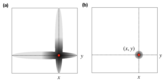
Figure 1: Schematic illustration of a fully factorized solution vs. an unfactorized solution. (a) is a factorized solution where the $x$ position is generated independently from the $y$ position of the Gaussian bump by intersecting two oval Gaussian bumps localized in one dimension but not the other. (b) shows a coupled solution where a single Gaussian bump localized in both dimension is generated. One difference between the two possibilities is that a network that recognized the independence of generation in $x,y$ could learn with $\mathcal{O}(2K)$ examples, while otherwise it would take $\mathcal{O}(K^{2})$ examples.

Specifically we conduct controlled experiments in this setting to investigate the following questions:

1. How does the representation learned by the model relate to its performance?

2. How and under what conditions do semantically meaningful representations emerge? How does training data affect the model’s learned representation?

3. Are the learned representations of the models factorized under imbalanced datasets?

1.2 Our Contributions

In this work, we aim to tackle the questions posed above via an empirical study of a toy conditional diffusion model using synthetic datasets that can be controllably varied. Our key findings can be summarized as follows:

• Diffusion models undergo three learning phases. We observe the three phases of manifold formation, including three distinct failure modes along the training progress.

• Performance is highly correlated with the learned representation. We find that the formation of an ordered manifold is a strong indicator of good model performance.

• Diffusion models learn semantically meaningful representations. In the terminal learning phase, a semantically meaningful representation emerges, and the rate at which it emerges depends on the data density.

• The learned representations are not efficient (factorized). We discover that even in imbalanced datasets with skewed representation of independent concepts, the learned manifold is not factorized.

Our work is the first empirical study to the best of our knowledge that demonstrates the phenomenology of manifold formation in the latent states and its phases in diffusion models by exploiting a toy model setting with controlled synthetic datasets. Our work demonstrates that a simple diffusion model with a standard architecture cannot learn an efficient representation, and hence warrants additional engineering efforts.

2 Experimental Setup

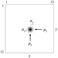
Figure 2: Example image data.

Dataset Generation. We generate 32 $\times$ 32 grayscale images each consisting of a single 2D spherical Gaussian bump at various locations of the image. The brightness of the pixel $v_{(x,y)}$ at position $(x,y)$ in a given image with a 2D Gaussian bump centered at $(\mu_{x},\mu_{y})$ with standard deviations of $(\sigma_{x},\sigma_{y})$ is given by $v_{(x,y)}=255\times(1-\exp{-(x-\mu_{x})^{2}/4\sigma_{x}^{2}-(y-\mu_{y})^{2}/4\sigma_{y}^{2}})$ with the normalized range of $v_{(x,y)}$ to be $[0,255]$. Each image is generated with a ground truth label of $(\mu_{x},\mu_{y})$, which continuously vary within $[0,32]^{2}$. In our convention of notation, we label the top left corner of the image as $(1,1)$ while the bottom right corner of the image as $(32,32)$. A sample image centered at $\mu_{x}=\mu_{y}=16$ with $\sigma_{x}=\sigma_{y}=1$ is shown in Fig. 2.

A dataset of these images consist of the enumeration of all possible Gaussians tiling the whole 32 $\times$ 32 canvas at increment $d_{x}$ in the $x$-direction and $d_{y}$ in the $y$-direction. A larger $d_{x}$ or $d_{y}$ means a sparser tiling of the image space and less abundant data while a smaller $d_{x}$ or $d_{y}$ result in more abundant data with denser tiling of the total image space. In a single dataset, we assume the spread of the Gaussian bump $\sigma_{x}=\sigma_{y}:=\sigma$ to be constant. With a larger spread leading to more spatial information of neighboring Gaussian bump and a smaller spread less information. By parameterically tuning the increments $d_{x}$ and $d_{y}$ and the spread $\sigma$, we can generate datasets of various sparsities and overlaps. We provide some a more detailed analysis of the various attributes of the data based on these parameters in Appendix Sec. A.5.

Models. We train a conditional Denoising Diffusion Probabilistic Models (DDPM) (Ho et al., 2020; Chen et al., 2021; Saharia et al., 2023) with a standard UNet architecture as shown in Fig. 6 in the Appendix. For each image in the training dataset, we provide an explicit ground truth label $(\mu_{x},\mu_{y})$ as the input to the embedding. For reference, we investigate the internal representation learned by the model using the output of layer 4 as labeled in Fig. 6. Since each dataset has inherently two latent dimensions, $x$- and $y$-positions, we use dimension reduction tools to reduce the internal representation of the model to a 3D embedding for the ease of visualization and analysis. We defer the details of model architecture, dimension reduction, and experimentation to Appendix Sections A.1 and  A.2.

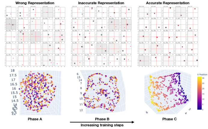
Figure 3: The three phases of manifold formation. The learned representations (UMAP reduced, colored by the ground truth $x$-positions) of the diffusion models undergo the three phases in increasing order of training steps as depicted in the 3D visualizations in the bottom row. In each phase, the corresponding qualitative generation behavior is demonstrated with 25 sampled images in the top row, in which the red dots mark the ground truth locations of the Gaussian bumps. (Phase A) has no particular structure in the learned representation, and the generated images either have no Gaussian bumps or multiple Gaussian bumps at the wrong locations. (Phase B) has a disordered, quasi-2D manifold with corresponding generation behavior of a single Gaussian bump at the wrong location. (Phase C) has an ordered 2D manifold with the desired generation behavior.

Evaluations. To briefly summarize, we assess the performance of the model based on the accuracies of the images generated and the quality of fit of the 3D embedding of the internal representation corresponding to the sampled images in predicting the ground truth image labels. We refer to the two quantitative performance indicators as the predicted label accuracy and the averaged R-squared. Intuitively, these two metrics range from 0 to 1, with the closer they are to 1 the higher quality of the generated images/learned representation, i.e., the better the performance of the model. Further details on these metrics can be found in Appendix Sec. A.3.

3 Results

Three phases in training. We train various diffusion models on datasets of various increments $d$ and $\sigma$ between the value of 0.1 to 1.0. For a fair comparison across these models, we fix the total amount of training steps for all models, as measured in units of batches (see Appendix Sec. A.6). As we increase the amount of training for a given model, we observe the universal emergence of three phases in manifold formation each corresponding to distinct generation behavior, as shown in Fig. 3. In particular, we noted three distinct failure modes during generation, namely i) no Gaussian bump is generated, ii) a single Gaussian bump is generated at an inaccurate location, and iii) multiple Gaussian bumps are generated at inaccurate locations. During the initial phase (phase A), the formed manifold does not have a particular structure or order. The generation behavior during this phase include all three of the above-mentioned failure modes. As we progressively increase the amount of training, we begin to witness phase B emerging, where the manifold formed is 2-dimensional or quasi-2D but unordered. The predominant failure mode of generation during this phase is ii, while the difference between the locations of the generated Gaussian bumps from their ground truths gradually diminishes as we proceed in training. Eventually, the model learns a 2D ordered manifold with the desired generation behavior, reaching the terminal phase C.

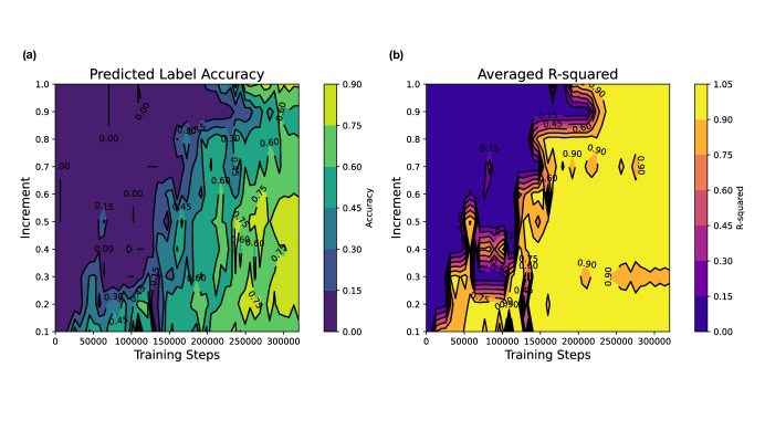
Figure 4: 2D phase diagram of performance metrics as a function of increment and training steps. (a) shows the predicted label accuracy and (b) shows the R-squared averaged in predicting $x$- and $y$-positions of the Gaussian bumps from the latent representation. The models are trained with datasets of various increments from 0.1 to 1.0 and sigma of 1.0. The total number of training steps are held constant across all the models.

Internal representation is key to performance. To investigate models’ performance and representations learned under various datasets, we plot the two performance metrics, accuracy and averaged R-squared, as a function of increasing increments and training steps in Fig. 4. For all datasets of varying increments, we have fixed the spread of the Gaussian bumps to be $\sigma=1.0$. Noticeably, comparing Fig. 4 (a) and (b) shows that learning a high-quality representation is key to achieving better accuracies in image generation. Moreover, in general, we observe that datasets with smaller increments lead to faster learning of the desired representation. Hence, given the same amount of training (having seen the same amount of data), the models trained using datasets that are more information-dense will result in a better-quality representation learned. On the other hand, with fewer data, an accurate representation can eventually be learned given enough training to compensate. We briefly comment on the information density of the datasets and discuss the trade-off between overlaps of neighboring Gaussian bumps and sensitivity to the spatial information encoded in Appendix Sec. A.5.

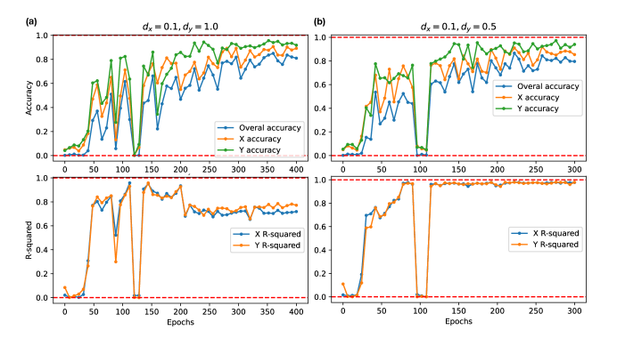
Figure 5: Performance metrics of models trained using imbalanced datasets. (a) using increments of $d_{x}=0.1$ and $d_{y}=1.0$ and (b) using increments of $d_{x}=0.1$ and $d_{y}=0.5$. Models in both cases are trained with amply sufficient amount of steps to reach convergence.

The learned manifold is not factorized. Finally, we answer the question of whether the representation learned is factorized. To test that, we train models on datasets that have imbalanced increments in the $x$-direction $d_{x}$ compared to the y-direction $d_{y}$. Given such a dataset, we would expect that the model learn these independent concepts at different rates based on the conclusion from Fig. 4, resulting in a factorized manifold. We tested two scenarios, one of stronger imbalance $d_{x}=0.1$ and $d_{y}=1.0$, and one of weaker imbalance $d_{x}=0.1$ and $d_{y}=0.5$. The performance metrics of the experiments in both cases are shown in Fig. 5(a) and (b), respectively. We see from the figures that despite having more data with finer-grained information of the $x$-positions, the accuracy of generating Gaussian bumps at the correct $y$ locations is generally higher than that at generating at the correct $x$ locations. Moreover, the R-squared values in fitting to the $x$- and the $y$-positions are strongly correlated, which is indicative that the representations learned are coupled rather than factorized. Overall, we observe that an imbalance in the dataset leads to a deterioration in the general performance of the model rather than factorizing the independent concepts.

4 Related Work

Compositional generalization has been empirically investigated in many deep generative models before  (Zhao et al., 2018; Xu et al., 2022; Okawa et al., 2023). Specifically, Zhao et al. (2018) investigated how inductive biases in GANs and VAEs affect their ability to compositionally generalize on toy cognitive psychological tasks. Similarly, Xu et al. (2022) developed an evaluation protocol to assess the performance of several unsupervised representation learning algorithms in compositional generalization, where they discovered that disentangled representations do not guarantee better generalization. In a recent empirical study of toy diffusion models, Okawa et al. (2023) shows that diffusion models learn to compositionally generalize multiplicatively. They, however, did not focus on the mechanistic aspect of the learning dynamics or analyze the representations learned by the models.

One alternative direction is engineering inductive biases that encourage the emergence of compositionality in diffusion models and beyond (Esmaeili et al., 2019; Higgins et al., 2018; Du et al., 2021; Yang et al., 2023; Du et al., 2023). Yang et al. (2023) applied disentangled representation learning techniques to diffusion models to automatically discover concepts and disentangle the gradient field of DDPMs into sub-gradient fields conditioned in the discovered factors. Along a similar line, Du et al. (2021) proposed an unsupervised scheme for discovering and representing concepts as separate energy functions that enables explicit composition and permutation of those concepts. In a series of follow-up works, Liu et al. (2021; 2022; 2023) explored compositional generation with composable diffusion and energy models, as well as concept discovery in text-to-image models.

5 Conclusion

Do diffusion models learn semantically meaningful and efficient representations? We conduct a well-controlled toy model study for diffusion models to learn to generate 2D Gaussian bumps at various $x$- and $y$-positions, given datasets that are parametrically generated to have various densities and overlaps. Throughout the learning process, we observe three phases of the manifold formation and identify corresponding generation behavior with distinctive failure modes in each phase. By comparing models trained under datasets of different sizes and overlaps, we conclude that learning a semantically meaningful representation is essential to model’s performance. Moreover, we observed that models learned a coupled representation of the independent latent features despite trained using imbalanced datasets. This leads us to conclude that a naïve architecture of diffusion models do not have the inductive bias that favors the emergence of disentangled/factorized representation. Hence, further investigation on how to learn factorized representation is warranted. A potential future direction would be to analyze biases that could enable the learning and generation of factorized representations in diffusion models and beyond in a controlled setting to better understand and overcome some of the limitations of current deep generative models in compositional generalization.

Acknowledgments

We thank Yilun Du for helpful discussions at the preliminary stage of our work.

Appendix A Experimental Details

A.1 Architecture

We train a conditional Denoising Diffusion Probabilistic Models (DDPM) Ho et al. (2020) with a standard UNet architecture of 3 downsampling and upsampling blocks, interlaced self-attention layers, and skip connections as shown in Fig. 6. Each down/up-sampling blocks consist of max pooling/upsampling layers followed by two double convolutional layers made up by convolutional layers, group normalization, and GELU activation functions.

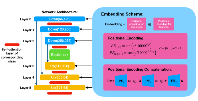
Figure 6: The UNet architecture of the conditional diffusion model. The schematic diagram of the standard UNet architecture consisting of three downsampling/upsampling blocks with interlaced self-attention layers and skip connections is shown on the left. The conditional information consisting of a concatenation of positional encodings of timestep and $x$/$y$-positions is passed in at each block as shown on the right.

The conditional information is passed in at each down/up-sampling block as shown in the schematic drawing. In our experiments, we choose to preserve the continuity of the Gaussian bump position labels passed into the model via positional encoding rather than using a separate trainable embedding layer at each block. Each embedding vector is made by concatenating equal length vectors of the positional encodings of the timestep, the $x$-position, and the $y$-position.

In our experiments, we visualize the outputs of layer 4 as the internal representation of the diffusion model. We have chosen not to use the output of the bottleneck layer for our study of the learned latent manifold, as we have observed that the bottleneck layers have diminishing signals in most of our experiments.

A.2 Dimension Reduction

We primarily use the dimension reduction technique Uniform Manifold Approximation and Projection for Dimension Reduction (UMAP) McInnes & Healy (2018) to study and visualize the learned representation of the model. Specifically, we collect image samples and their corresponding internal representations (outputs of layer 4 from the architecture described in Sec. A.1). We then transform the high-dimensional internal representations into a 3D embedding as a sample of the learned representation, which we visualize and analyze. For an implementation of UMAP, we used the Python package McInnes et al. (2018).

A.3 Evaluation

We assess the performance of the model using two primary criteria: 1) the quality of the denoised images and 2) the quality of the learned representation.

At a given time during or after training, we generate 500 denoised images and their corresponding internal representations of randomly sampled labels based on the training dataset. We predict the labels from the image generated based on the $x$- and $y$-positions of the generated Gaussian bump in the image. We then compute the accuracy of predicted labels from the ground truth labels averaged over 500 samples as

$$\text{Accuracy}=\frac{1}{500}\sum_{i=1}^{500}\bm{1}(|\mu^{i}_{x}-\hat{\mu}^{i}_{x}|<1)\cdot\bm{1}(|\mu^{i}_{y}-\hat{\mu}^{i}_{y}|<1),$$ (1)

where $\bm{1}(\cdot)$ is an indicator function that returns 1 if the expression within holds true, 0 otherwise. Similarly, we can modify this expression to only assess the accuracy of generated $x$-positions or $y$-positions separately. Here we estimate the center of the Gaussian bump $\hat{\mu}^{i}_{x}$ and $\hat{\mu}^{i}_{y}$ using a label prediction algorithm described in Alg. 1 implemented using Otsu’s image thresholding and the contour-finding algorithm in the OpenCV package, abbreviated as cv2. In the cases where there are no bumps or more than one bump, the algorithm defaults back to finding the centroid of the image.

Algorithm 1 Label prediction algorithm

1:function LabelPrediction(img)

2:     $(T,\text{thresh})\leftarrow\text{cv2.threshold}(\text{img},0,255,\text{cv2.THRESH\_BINARY\_INV}\,|\,\text{cv2.THRESH\_OTSU})$

3:     $\text{contours},\_\leftarrow\text{cv2.findContours}(\text{thresh},\text{cv2.RETR\_ExTERNAL},\text{cv2.CHAIN\_APPROx\_SIMPLE})$

4:     if $\text{len(contours)}=0$ or $\text{len(contours)}>1$ then

5:         return ComputeCentroid2D(img)

6:     end if

7:     $\text{max\_contour}\leftarrow\text{max(contours, key=cv2.contourArea)}$

8:     $(x,y,w,h)\leftarrow\text{cv2.boundingRect}(\text{max\_contour})$

9:     $cx\leftarrow x+\frac{w}{2}$

10:     $cY\leftarrow y+\frac{h}{2}$

11:     return $(cx,cY)$

12:end function

To assess the quality of the learned representation, we perform two 1D linear regressions on the UMAP-reduced 3D embedding of the internal representations (outputs of layer 4) corresponding to the 500 sampled images. We use the R-squared values of fit in both predicting $\mu_{x}$ and $\mu_{y}$ as an indicator for the quality of the manifold learned in representing $x$- and $y$-positions of the Gaussian bumps.

A.4 Training Loss

Diffusion models iteratively denoise a Gaussian noisy image $\mathbf{x}_{T}$ into a noisefree image $\mathbf{x}_{0}$ over diffusion timesteps $t\in\{0,1,\ldots,T\}$ given the forward distribution $q(\mathbf{x}_{t}|\mathbf{x}_{t-1})$ by learning the reverse distribution $p_{\theta}(\mathbf{x}_{t-1}|\mathbf{x}_{t})$. Given a conditional cue $\mathbf{c}$, a conditional diffusion model (Chen et al., 2021; Saharia et al., 2023) reconstructs an image from a source distribution $q(\mathbf{x}_{0}|\mathbf{c})$. Specifically, we train our neural network (UNet) to predict the denoising direction $\epsilon_{\theta}(\mathbf{x}_{t},t,\mathbf{c})$ at a given timestep $t$ with conditional cue $\mathbf{c}$ with the goal of minimizing the mean squared loss (MSE) between the predicted and the ground truth noise $\epsilon$ as follows

$$\mathcal{L}:=\mathbb{E}_{t\in\{0,\ldots,T\},\mathbf{x}_{0}\sim q(x_{0}|\mathbf{c}),\epsilon\sim\mathcal{N}(\mathbf{0},\mathbf{I})}\left[\lVert\epsilon-\epsilon_{\theta}(\mathbf{x}_{0},t,\mathbf{c})\rVert^{2}\right],$$ (2)

where we assume each noise vector $\epsilon$ to be sampled from a Gaussian distribution $\mathcal{N}(\mathbf{0},\mathbf{I})$ I.I.D. at each timestep $t$.

A.5 Datasets

The datasets we used for training the models generating the results in Sec. 3 have various increments $d_{x}$/$d_{y}$ and $\sigma$. Here we briefly comment on the interplay between increments and sigmas, and how they affect dataset densities and overlaps. The ultimate goal of our task of interest is to learn a continuous 2D manifold of all possible locations of the Gaussian bumps. Our datasets are discrete approximations of continuous manifold that can be thought of as a “web” with each data point as a “knot,” a schematic illustration is shown in Fig. 7(a). Intuitively, the spatial information necessary for an organized, continuous, and semantically meaningful representation to emerge is encoded in the overlap of the neighboring Gaussian bumps, which is tuned via the parameters $d$ and $\sigma$. As we increase $d$, the size of the dataset gets scaled quadratically, resulting in each Gaussian bump to have more overlap with its neighbors.

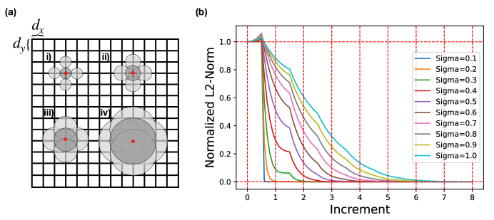
Figure 7: The overlap of Gaussian bumps with various spreads. (a) is a schematic demonstration the interplay between the increment $d_{x}$/$d_{y}$ and the spread of the Gaussians determined by $\sigma$. The labeled diagram i-iv) shows examples of having no overlap (no neighbor information), nearest neighbor overlap, nearest neighbor and adjacent overlap, and N-nearest neighbors overlap, respectively. (b) shows the normalized L2-norm of the inverted Gaussian image overlaps.

As we scale up $\sigma$, the dataset size remains fixed while the overlaps with neighbors are significantly increased. In Fig. 7(b), we plot the normalized L2-norm of the product image of neighboring Gaussian bumps as a function of increments for various spreads. Specifically, given two inverted grayscale Gaussian bump images, $a$ and $b$, the normalized L2-norm of their product is given by the formula $\lVert\sqrt{a*b}\rVert_{2}/\lVert a\rVert_{2}$, where $*$ is element-wise multiplication and $\lVert\cdot\rVert_{2}$ is the L2-norm. This quantity should give a rough measure of the image overlap with the exception at increment around 0.5 due to the discrete nature of our data. Moreover, we note that the cusps in the curves occur for the same reason. As we can see, the number of neighbors that a given Gaussian bump has non-trivial overlaps with grows roughly linearly to sub-linearly with the spread. Nonetheless, in Sec. B.1 we show that there is no strong correlation between performance or the rate at which semantically meaningful representations emerges and the spread of the Gaussian bumps.

A.6 Training Details

We train various diffusion models on datasets of various increments $d$ and $\sigma$ from the range $\{0.1,0.2,0.3,0.4,0.5,0.6,0.7,0.8,0.9,1.0\}$. For each model, we fix the total training steps to be 320,000 (number of epochs $\times$ the dataset size in units of batches). We train the models on a quad-core Nvidia A100 GPU, and an average training session lasts around 6 hours. For each model we run three separate seeds and select the run that achieve the optimal accuracy at terminal epoch. To produce the results shown in Fig. 4 and Fig. 8, we sample 500 images as well as their corresponding outputs at layer 4 every 6400 training steps and at the terminal step.

Appendix B Additional Results

B.1 The role of Sigma

Previously, in Appendix Sec. A.5, we have discussed how spatial information encoded in the datasets varies based on the increment $d$ and the spread $\sigma$. We show in Sec. 3 that indeed a smaller increment results in a faster rate of convergence leading to a semantically meaningful latent representation. In Fig. 8, we show the performance metrics as a function of sigma and training steps for three separate increments $d=0.1,0.5,1.0$. There is, however, no strong correlation between model performance and increasing sigma. One possible explanation for this could be the fact that changing sigma only results in a modest change in the dataset (linear to sub-linear in the number of overlapping neighbors), unlike changing increments, which results in a quadratic change in the dataset in addition to more fine-grained embeddings. Moreover, we noticed that for some seeds, some of the sigmas that we have tested do not learn a semantically meaningful manifold. This seed dependence issue is exacerbated with models trained using datasets of bigger increments.

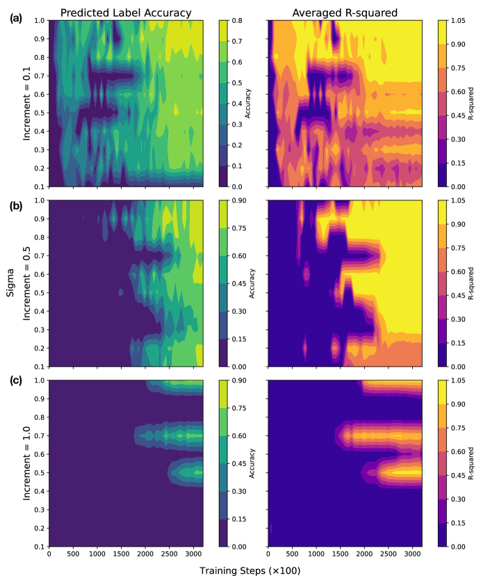
Figure 8: Phase diagrams of performance metrics as a function of sigmas and training steps for various increments. (a) Increment = 0.1, (b) Increment = 0.5, (c) Increment = 1.0.

B.2 Compositional Generalization Performance

Can the models compositionally generalize well? To answer this question, we train two models under an incomplete training dataset of $d=0.1$ and $\sigma=1.0$, where we deliberately “poke a hole” in the middle of the data manifold and see if the model can still learn an accurate representation. Fig. 9 shows the performance metrics of the model trained under $\sim 3.5\%$ (a smaller hole) and $\sim 10\%$ (a bigger hole). We note that given sufficient amount of training, both models were able to construct a semantically meaningful 2D representation, with the accuracy of the OOD only slightly worse off in the case where $\sim 10\%$ of the data is skipped as compared to that where only $\sim 3.5\%$ is skipped. In general, the models were able to successfully compositionally generalize, although the mechanism of how they do so warrants further investigation.

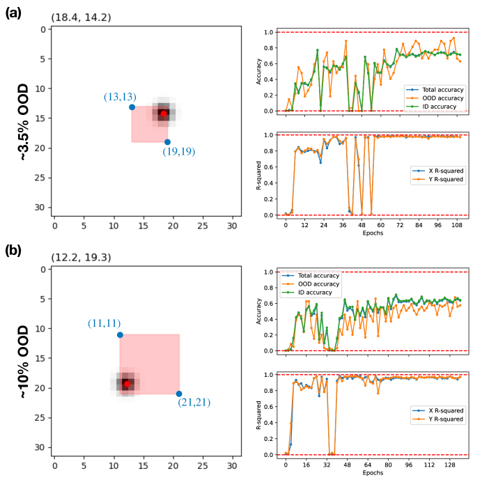
Figure 9: Performance metrics of models trained under an incomplete set of training data. Both models are trained using a dataset of $d=0.1$ and $\sigma=1.0$, with (a) $\sim 3.5\%$ and (b) $\sim 10\%$ of the training dataset skipped during training. The training data images with Gaussian bumps centered within the red-shaded regions in the sample OOD images shown on the left are skipped during training.

References

- Chen et al. (2021) Nanxin Chen, Yu Zhang, Heiga Zen, Ron J. Weiss, Mohammad Norouzi, and William Chan. Wavegrad: Estimating gradients for waveform generation. In 9th International Conference on Learning Representations, ICLR 2021, Virtual Event, Austria, May 3-7, 2021. OpenReview.net, 2021. URL https://openreview.net/forum?id=NsMLjcFaO8O.
- Du et al. (2021) Yilun Du, Shuang Li, Yash Sharma, Josh Tenenbaum, and Igor Mordatch. Unsupervised learning of compositional energy concepts. In Marc’Aurelio Ranzato, Alina Beygelzimer, Yann N. Dauphin, Percy Liang, and Jennifer Wortman Vaughan (eds.), Advances in Neural Information Processing Systems 34: Annual Conference on Neural Information Processing Systems 2021, NeurIPS 2021, December 6-14, 2021, virtual, pp. 15608–15620, 2021. URL https://proceedings.neurips.cc/paper/2021/hash/838aac83e00e8c5ca0f839c96d6cb3be-Abstract.html.
- Du et al. (2023) Yilun Du, Conor Durkan, Robin Strudel, Joshua B. Tenenbaum, Sander Dieleman, Rob Fergus, Jascha Sohl-Dickstein, Arnaud Doucet, and Will Sussman Grathwohl. Reduce, reuse, recycle: Compositional generation with energy-based diffusion models and MCMC. In Andreas Krause, Emma Brunskill, Kyunghyun Cho, Barbara Engelhardt, Sivan Sabato, and Jonathan Scarlett (eds.), International Conference on Machine Learning, ICML 2023, 23-29 July 2023, Honolulu, Hawaii, USA, volume 202 of Proceedings of Machine Learning Research, pp. 8489–8510. PMLR, 2023. URL https://proceedings.mlr.press/v202/du23a.html.
- Esmaeili et al. (2019) Babak Esmaeili, Hao Wu, Sarthak Jain, Alican Bozkurt, N. Siddharth, Brooks Paige, Dana H. Brooks, Jennifer G. Dy, and Jan-Willem van de Meent. Structured disentangled representations. In Kamalika Chaudhuri and Masashi Sugiyama (eds.), The 22nd International Conference on Artificial Intelligence and Statistics, AISTATS 2019, 16-18 April 2019, Naha, Okinawa, Japan, volume 89 of Proceedings of Machine Learning Research, pp. 2525–2534. PMLR, 2019. URL http://proceedings.mlr.press/v89/esmaeili19a.html.
- Higgins et al. (2018) Irina Higgins, Nicolas Sonnerat, Loic Matthey, Arka Pal, Christopher P. Burgess, Matko Bosnjak, Murray Shanahan, Matthew M. Botvinick, Demis Hassabis, and Alexander Lerchner. SCAN: learning hierarchical compositional visual concepts. In 6th International Conference on Learning Representations, ICLR 2018, Vancouver, BC, Canada, April 30 - May 3, 2018, Conference Track Proceedings. OpenReview.net, 2018. URL https://openreview.net/forum?id=rkN2Il-RZ.
- Ho et al. (2020) Jonathan Ho, Ajay Jain, and Pieter Abbeel. Denoising diffusion probabilistic models. In Hugo Larochelle, Marc’Aurelio Ranzato, Raia Hadsell, Maria-Florina Balcan, and Hsuan-Tien Lin (eds.), Advances in Neural Information Processing Systems 33: Annual Conference on Neural Information Processing Systems 2020, NeurIPS 2020, December 6-12, 2020, virtual, 2020. URL https://proceedings.neurips.cc/paper/2020/hash/4c5bcfec8584af0d967f1ab10179ca4b-Abstract.html.
- Liu et al. (2021) Nan Liu, Shuang Li, Yilun Du, Josh Tenenbaum, and Antonio Torralba. Learning to compose visual relations. In Marc’Aurelio Ranzato, Alina Beygelzimer, Yann N. Dauphin, Percy Liang, and Jennifer Wortman Vaughan (eds.), Advances in Neural Information Processing Systems 34: Annual Conference on Neural Information Processing Systems 2021, NeurIPS 2021, December 6-14, 2021, virtual, pp. 23166–23178, 2021. URL https://proceedings.neurips.cc/paper/2021/hash/c3008b2c6f5370b744850a98a95b73ad-Abstract.html.
- Liu et al. (2022) Nan Liu, Shuang Li, Yilun Du, Antonio Torralba, and Joshua B. Tenenbaum. Compositional visual generation with composable diffusion models. In Shai Avidan, Gabriel J. Brostow, Moustapha Cissé, Giovanni Maria Farinella, and Tal Hassner (eds.), Computer Vision - ECCV 2022 - 17th European Conference, Tel Aviv, Israel, October 23-27, 2022, Proceedings, Part XVII, volume 13677 of Lecture Notes in Computer Science, pp. 423–439. Springer, 2022. doi: 10.1007/978-3-031-19790-1“˙26. URL https://doi.org/10.1007/978-3-031-19790-1_26.
- Liu et al. (2023) Nan Liu, Yilun Du, Shuang Li, Joshua B. Tenenbaum, and Antonio Torralba. Unsupervised compositional concepts discovery with text-to-image generative models. In IEEE/CVF International Conference on Computer Vision, ICCV 2023, Paris, France, October 1-6, 2023, pp. 2085–2095. IEEE, 2023. doi: 10.1109/ICCV51070.2023.00199. URL https://doi.org/10.1109/ICCV51070.2023.00199.
- McInnes & Healy (2018) Leland McInnes and John Healy. UMAP: uniform manifold approximation and projection for dimension reduction. CoRR, abs/1802.03426, 2018. URL http://arxiv.org/abs/1802.03426.
- McInnes et al. (2018) Leland McInnes, John Healy, Nathaniel Saul, and Lukas Grossberger. Umap: Uniform manifold approximation and projection. The Journal of Open Source Software, 3(29):861, 2018.
- Okawa et al. (2023) Maya Okawa, Ekdeep Singh Lubana, Robert P. Dick, and Hidenori Tanaka. Compositional abilities emerge multiplicatively: Exploring diffusion models on a synthetic task. CoRR, abs/2310.09336, 2023. doi: 10.48550/ARXIV.2310.09336. URL https://doi.org/10.48550/arXiv.2310.09336.
- Ramesh et al. (2021) Aditya Ramesh, Mikhail Pavlov, Gabriel Goh, Scott Gray, Chelsea Voss, Alec Radford, Mark Chen, and Ilya Sutskever. Zero-shot text-to-image generation. In International Conference on Machine Learning, pp. 8821–8831. PMLR, 2021.
- Rombach et al. (2022) Robin Rombach, Andreas Blattmann, Dominik Lorenz, Patrick Esser, and Björn Ommer. High-resolution image synthesis with latent diffusion models. In Proceedings of the IEEE/CVF conference on computer vision and pattern recognition, pp. 10684–10695, 2022.
- Saharia et al. (2022) Chitwan Saharia, William Chan, Saurabh Saxena, Lala Li, Jay Whang, Emily L Denton, Kamyar Ghasemipour, Raphael Gontijo Lopes, Burcu Karagol Ayan, Tim Salimans, et al. Photorealistic text-to-image diffusion models with deep language understanding. Advances in Neural Information Processing Systems, 35:36479–36494, 2022.
- Saharia et al. (2023) Chitwan Saharia, Jonathan Ho, William Chan, Tim Salimans, David J. Fleet, and Mohammad Norouzi. Image super-resolution via iterative refinement. IEEE Trans. Pattern Anal. Mach. Intell., 45(4):4713–4726, 2023. doi: 10.1109/TPAMI.2022.3204461. URL https://doi.org/10.1109/TPAMI.2022.3204461.
- Xu et al. (2022) Zhenlin Xu, Marc Niethammer, and Colin Raffel. Compositional generalization in unsupervised compositional representation learning: A study on disentanglement and emergent language. In Sanmi Koyejo, S. Mohamed, A. Agarwal, Danielle Belgrave, K. Cho, and A. Oh (eds.), Advances in Neural Information Processing Systems 35: Annual Conference on Neural Information Processing Systems 2022, NeurIPS 2022, New Orleans, LA, USA, November 28 - December 9, 2022, 2022. URL http://papers.nips.cc/paper_files/paper/2022/hash/9f9ecbf4062842df17ec3f4ea3ad7f54-Abstract-Conference.html.
- Yang et al. (2023) Tao Yang, Yuwang Wang, Yan Lv, and Nanning Zheng. Disdiff: Unsupervised disentanglement of diffusion probabilistic models. CoRR, abs/2301.13721, 2023. doi: 10.48550/ARXIV.2301.13721. URL https://doi.org/10.48550/arXiv.2301.13721.
- Zhao et al. (2018) Shengjia Zhao, Hongyu Ren, Arianna Yuan, Jiaming Song, Noah D. Goodman, and Stefano Ermon. Bias and generalization in deep generative models: An empirical study. In Samy Bengio, Hanna M. Wallach, Hugo Larochelle, Kristen Grauman, Nicolò Cesa-Bianchi, and Roman Garnett (eds.), Advances in Neural Information Processing Systems 31: Annual Conference on Neural Information Processing Systems 2018, NeurIPS 2018, December 3-8, 2018, Montréal, Canada, pp. 10815–10824, 2018. URL https://proceedings.neurips.cc/paper/2018/hash/5317b6799188715d5e00a638a4278901-Abstract.html.