Less is KEN: a Universal and Simple Non-Parametric Pruning Algorithm for Large Language Models

Abstract

Neural network pruning has become increasingly crucial due to the complexity of neural network models and their widespread use in various fields. Existing pruning algorithms often suffer from limitations such as architecture specificity, excessive complexity and reliance on complex calculations, rendering them impractical for real-world applications. In this paper, we propose KEN: a straightforward, universal and unstructured pruning algorithm based on Kernel Density Estimation (KDE). KEN aims to construct optimized transformer models by selectively preserving the most significant parameters while restoring others to their pre-training state. This approach maintains model performance while allowing storage of only the optimized subnetwork, leading to significant memory savings. Extensive evaluations on seven transformer models demonstrate that KEN achieves equal or better performance than the original models with a minimum parameter reduction of 25%. In-depth comparisons against other pruning and PEFT algorithms confirm KEN effectiveness. Furthermore, we introduce KEN_viz, an explainable tool that visualizes the optimized model composition and the subnetwork selected by KEN.

1 Introduction

Large Language Models (LLMs) have become the best and simplest solution for achieving state-of-the-art results in many natural language processing (NLP) applications. However, the increasing use of neural networks (NNs) and transformer models Vaswani et al. (2017) has resulted in a rise in computational cost due to the complexity of arithmetic calculations, larger matrices and the addition of more layers. Consequently, the weight and structure of these models become more complex, requiring high demands in computation and memory.

One of the best approaches to address the overwhelming size of LLMs is to reduce their resources through pruning algorithms. These algorithms can eliminate parameters or entire components in a NN, making it lighter without compromising its original performance. Pruning algorithms emerged in parallel with the earliest use of NNs Mozer and Smolensky (1989); Janowsky (1989); LeCun et al. (1989), but they have gained significant importance in the last decade due to the widespread use of these networks in various fields. There are many pruning algorithms in literature Blalock et al. (2020), each with a unique approach or adapted old algorithms for these new architectures Benbaki et al. (2023). However, the complexity of neural networks can pose a challenge when creating pruning algorithms, as these may require creating new complex theories to make the models lightweight Dong et al. (2017); Malach et al. (2020). Additionally, existing pruning algorithms often exhibit shortcomings in their completeness Blalock et al. (2020) and fail to consider a critical aspect: the efficient storage of the pruned model. Some algorithms compress the model at runtime, but they lack a mechanism to persist the reduced NN for future use. Therefore, most algorithms in the literature focus only on the speed at which they reduce and execute the model without considering this crucial final stage. This is particularly important in resource-limited environments that use neural networks, such as smart devices and mobile phones Yang et al. (2017); Sze et al. (2017).

This paper presents KEN (Kernel density Estimator for Neural network compression): a universal, simple, magnitude-based transformer pruning algorithm that leverages Kernel Density Estimation (KDE) for parameter pruning. In contrast to other pruning methods that rely on loss function minimization or exhaustive parameter search, KEN utilizes KDEs to identify and retain the most influential parameters while resetting the remaining ones to their original pre-trained values. This innovative pruning strategy streamlines the optimization process by leveraging the natural distribution of model parameters, eliminating any architecture-specific considerations. KEN effectively reduces the size of transformer models by a minimum of 25% without compromising performance. The pruned models consist solely of a subnetwork of trained parameters, which can be seamlessly downloaded and injected into pre-trained models on demand. This feature enables dynamic model reconfiguration and saves significant memory space that would otherwise be needed to store the fully trained model. Comparative evaluations demonstrate KEN exceptional capabilities, surpassing existing transformer pruning and PEFT algorithms. Additionally, we introduce KEN_viz: an explainable tool that graphically depicts the optimized model from various perspectives. KEN_viz highlights the KEN-selected parameters, their layer-wise differences and neighbor counts for each matrix that made up the analyzed model. Using KEN, we employed a non-parametric method widely used in statistics to create an efficient and intuitive pruning algorithm. Our approach achieved excellent results in terms of efficiency and performance, making it a practical alternative to other more complex pruning algorithms.

2 Background

Compression algorithms can be summarized in three areas of research: weight pruning Han et al. (2015); Zhu and Gupta (2017), quantization Gong et al. (2014); Zhu et al. (2016) and knowledge distillation Ba and Caruana (2014); Kim and Rush (2016). These techniques aim to make models lighter, but each of them takes a different approach. Weight pruning removes model parameters according to the chosen algorithm and strategy, while quantization reduces the number of bits necessary to represent each parameter. Knowledge distillation, instead, tries to minimize the learned large knowledge of a model into a smaller one without affecting its validation.

Focusing on pruning algorithms, there are different approaches depending on the strategy and algorithm adopted. Pruning algorithms can be classified as either structured or unstructured, based on the approach applied and magnitude-based or impact-based, according to the algorithm used. Structured pruning Huang et al. (2018); Wang et al. (2019); Gordon et al. (2020) removes weights in groups, such as entire neurons, filters or layers, while unstructured pruning Han et al. (2015); Frankle and Carbin (2018); Lagunas et al. (2021); Benbaki et al. (2023) does not consider any relationship between parameters and selects weights to prune based on their impact or magnitude. Magnitude-based algorithms Hanson and Pratt (1988); Mozer and Smolensky (1989); Gordon et al. (2020) analyze the absolute value of each parameter to determine its importance. In contrast, impact-based algorithms LeCun et al. (1989); Hassibi and Stork (1992); Singh and Alistarh (2020) work on the loss function and its variation caused by removing a parameter. The winning ticket hypothesis Frankle and Carbin (2018), is a recent advancement in pruning techniques. A winning ticket is a subnetwork within a trained model that - when trained in isolation - can achieve performance comparable to the original model even after significant pruning. To identify the winning ticket, a pruning criterion is applied to zero-mask weights and the remaining network is retrained. This process can be repeated multiple times or in a one-shot manner.

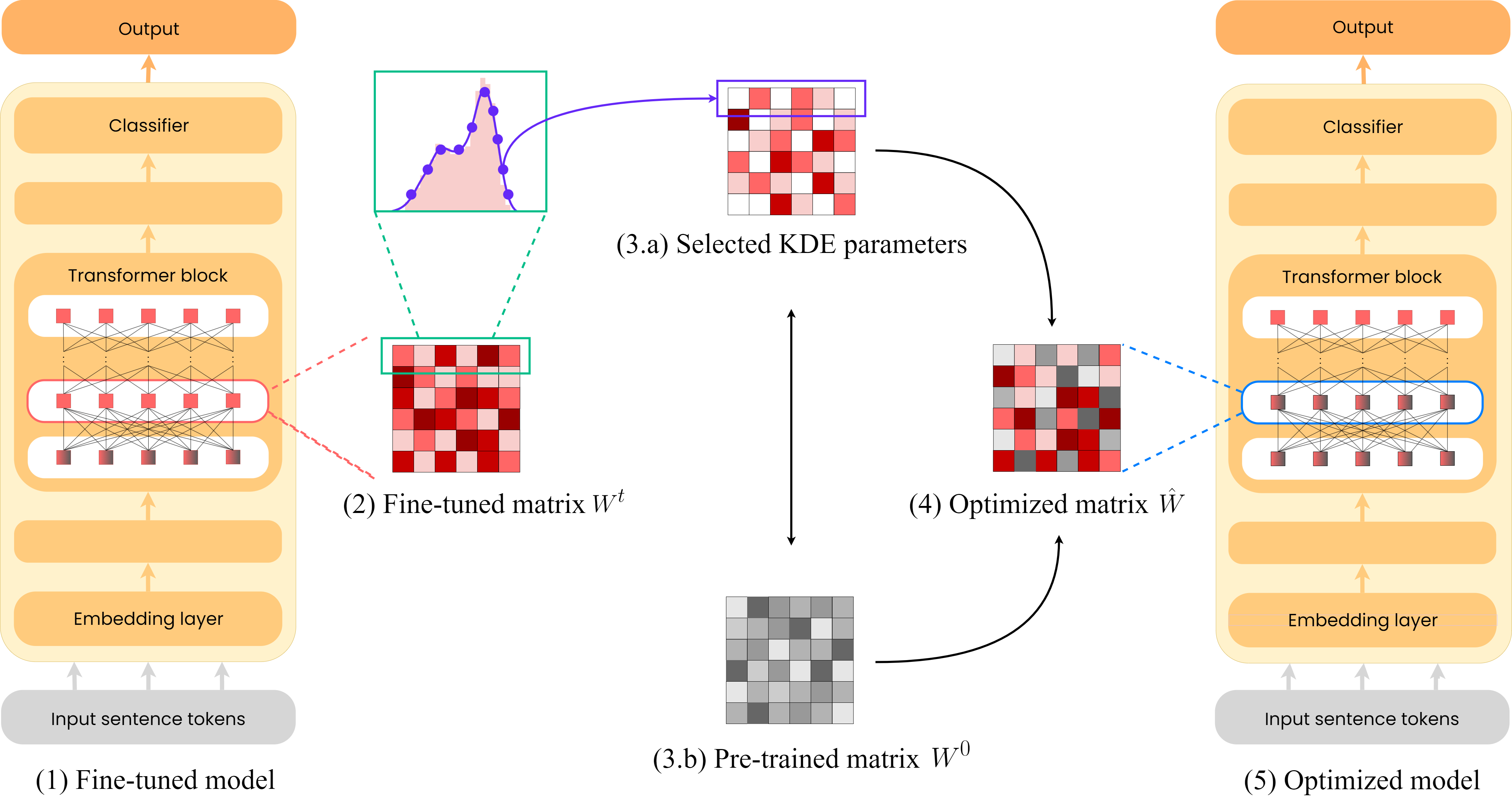
Figure 1: KEN workpath: From a fine-tuned model (1), for each of its fine-tuned matrices (2), the row distribution and the respective KDE (Kernel Density Estimator) are calculated. All values within the KDE are selected (3.a), while the remainder are restored to their pre-tuned value (3.b). The resulting optimized matrix (4) is then fed back into the model (5)

3 Related Work

In this section, we present three algorithms that are relevant benchmarks for our proposed algorithm, KEN. These algorithms have some similarities with it: the first two, called FLOP and BMP, are pruning algorithms designed to reduce the size of transformer models by employing algebraic or geometric techniques. The third, LoRA is the SoTA parameter-efficient algorithm for LLMs.

Factorized Low-rank Pruning

(FLOP: Wang et al., 2019) FLOP is a magnitude-based pruning algorithm that employs matrix factorization to reduce the size of matrices in transformer models. This approach involves decomposing each matrix into smaller rank-1 components, which are then multiplied together to form the original matrix. For attention layers, FLOP decomposes each matrix into smaller rank-1 components based on the magnitudes of the matrix entries. For embedding layers, FLOP adaptively prunes dimensions based on word clusters. This means that FLOP only prunes dimensions that are not frequently used Joulin et al. (2017); Bastings et al. (2019), which helps to reduce the model size without sacrificing performance.

Block Movement Pruning

(BMP: Lagunas et al., 2021) introduces an extension to the movement pruning technique used in transformers Sanh et al. (2020). This approach reduces the size of each matrix in a transformer model by dividing it into fixed-sized blocks. Regularization is then applied, and the NN is trained through distillation to match the performance of a teacher model. Our focus is on two pruning methods: Hybrid and HybridNT. The key difference between these two approaches is that HybridNT does not involve the use of a teacher model during training (No Teacher).

Low-Rank Adaptation of Large Language Models

(LoRA: Hu et al., 2021) LoRA is a novel fine-tuning method that leverages low-rank decomposition to reduce the parameter size of large language models (LLMs) while preserving their performance. This approach involves decomposing the LLMs weight matrices into low-rank components, which are then fine-tuned along with the original weights. This approach enables efficient parameter adaptation to specific tasks without compromising the LLMs generalization capabilities.

4 KEN pruning algorithm

KEN (Kernel density Estimator for Neural network compression) pruning algorithm is designed to identify and extract the most essential subnetwork from each transformer model following the main idea of the winning ticket hypothesis Frankle and Carbin (2018). This algorithm effectively prunes the network by employing Kernel Density Estimators (KDEs), retaining only the essential parameters and resetting the rest to their pre-trained values. The optimized subnetwork can be stored independently and seamlessly integrated into its pre-trained configuration for downstream applications.

KEN utilizes KDE to generalize the point distribution of each transformer matrix, resulting in a lightweight and smooth version of the original fine-tuned model. To prevent the complete deconstruction of the initial matrix composition, KEN applies KDE to the individual rows. The KDE calculation requires a $k$ value, which defines the number of points employed in the distribution calculation. Consequently, the $k$ value determines the number of the selected fine-tuned parameters, thus a lower $k$ value indicates a closer resemblance to the pre-trained model while a higher $k$ value reflects a closer alignment with its fine-tuned version.

The KEN algorithm can be described using the three phases defined below:

Phase 1: Parameter Extraction and KDE Calculation

Given a pre-trained matrix $W^{0}$ of a fixed layer $l$:

$$W^{0}=\{w_{1,1}^{0},...,w_{n,m}^{0}\}\quad|\quad W^{0}\in\mathbb{R}^{n\times m}$$

and its corresponding fine-tuned counterpart $W^{t}$:

$$W^{t}=\{w_{1,1}^{t},...,w_{n,m}^{t}\}\quad|\quad W^{t}\in\mathbb{R}^{n\times m}$$

For each row $r_{i}^{t}$ of the fine-tuned matrix $W^{t}$:

$$r_{i}^{t}=\{w_{i,1}^{t},...,w_{i,m}^{t}\}\quad\forall i\in[1,n]$$

KEN calculates the KDE distribution of the row $r_{i}^{t}$ using a bandwidth parameter $h$ determined following Scott’s rule of thumb Scott (2015).

$$h=1.06\cdot\hat{\sigma}\cdot n^{-\frac{1}{5}}$$

where $\hat{\sigma}$ is the standard deviation of $r_{i}^{t}$.

Phase 2: Parameter Retention and Pre-trained Value Reset

Using the KDE likelihood, the $k$ points that best fit the $r_{i}^{t}$ row distribution are identified, while the others are reset to their pre-trained values. This process results in an optimized row $\hat{r}_{i}$:

$$\hat{r}_{i}=\{\hat{w}_{i,1},...,\hat{w}_{i,m}\}\quad\forall i\in[1,n]$$

computed using the following binary function:

$$f(\hat{w}_{i,j})=\begin{cases}w_{i,j}^{t}\hskip 5.69046pt$if$\quad w_{i,j}^{t}\in\hskip 5.69046pt$KDE \hskip 5.69046ptlikelihood$\\ w_{i,j}^{0}\quad$otherwise$\end{cases}\$$ (1)

Phase 3: Matrix Replacement and Optimized Fine-tuned Model

After applying the previous step on each row, the optimized matrix $\hat{W}$:

$$\hat{W}=\{\hat{w}_{1,1},...,\hat{w}_{n,m}\}\quad|\quad\hat{W}\in\mathbb{R}^{n\times m}$$

will replace the original fine-tuned matrix $W^{t}$ within the model.

KEN operates iteratively, replacing the $W^{t}$ matrix with $\hat{W}$ during each iteration. So, after the t-th iteration, the model will have t-optimized matrices, effectively replacing the fine-tuned matrices without creating any additional versions of the model. This versatility allows KEN to prune the entire model or specific layer ranges.

Data: $W^{0}=\{w_{1,1}^{0},...,w_{n,m}^{0}\}$, $W^{t}=\{w_{1,1}^{t},...,w_{n,m}^{t}\},k$

Result: $\hat{W}$

$\hat{W}[n,m]\leftarrow 0$

for i = 1 to n do

       $\texttt{best\_points}\leftarrow KDE(r_{i}^{t},k)$

      for j = 1 to m do

             $\hat{r}_{i}^{t}\leftarrow[]$

            if $r_{i}^{t}[j]$ in best_points then

                   $\hat{r}_{i}^{t}[j]\leftarrow r_{i}^{t}[j]$

            else

                   $\hat{r}_{i}^{t}[j]$$\leftarrow r_{i}^{0}[j]$

             end if

            

       end for

      $\hat{W}[i]\leftarrow\hat{r}_{i}^{t}$

end for

return $\hat{W}$

Algorithm 1 Generate the optimized $\hat{W}$ matrix using KEN

Alg. 1 explains more formally all the three phases described to generate the optimized matrix $\hat{W}$. Additionally, the graphical representation displayed in Fig. 1 provides a clear and comprehensive visualization of all KEN steps while Fig.2 shows different $\hat{W}$ matrices obtained using different $k$ values.

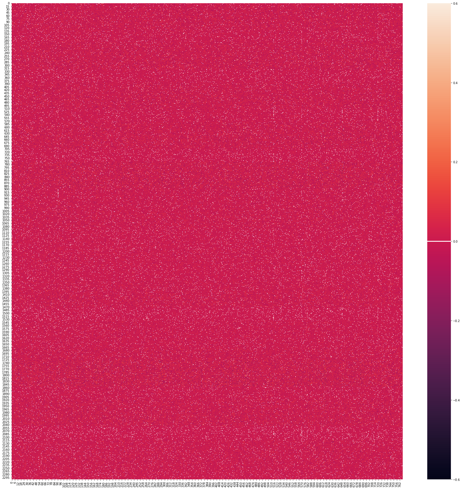
(a) Fine-tuned matrix

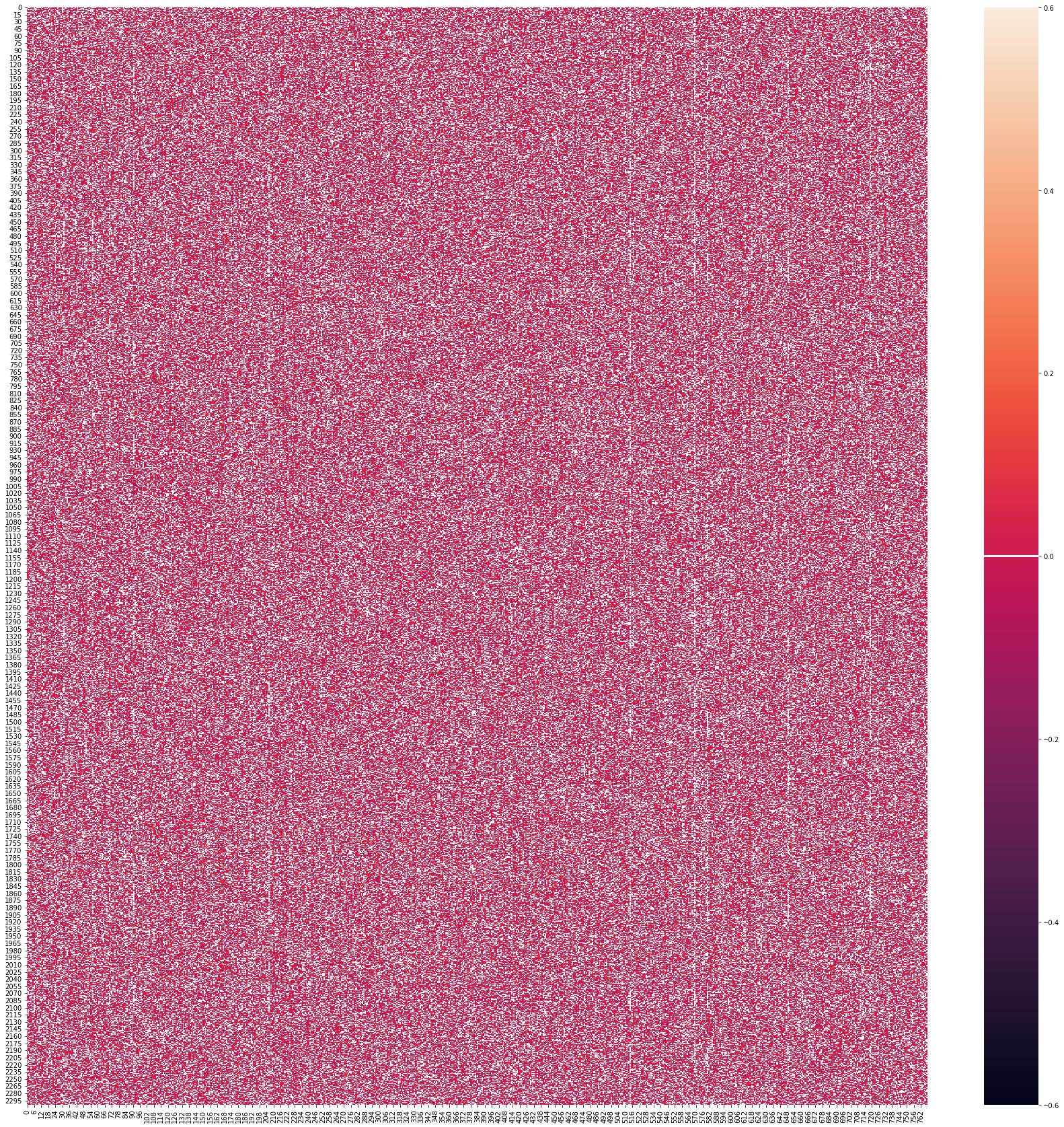
(b) Reset params 34.90%

(c) Reset params: 60.94%

(d) Reset params: 86.98%

Figure 2: Comparing the impact of KEN parameter selection on the same fine-tuned matrix (a). Matrix (a) represents the in_proj matrix at layer 0 of a DeBERTa model trained on the AG_NEWS dataset. No selected parameters are blank

5 Experiments

To validate our algorithm, we conducted a series of extensive case studies. Sec. 5.1 describes the experimental setup, including the models employed and the $k$ values tested. Additionally, Sec. 5.2 focused on investigating the feasibility of saving and loading compressed data.

5.1 Experimental set-up

To evaluate KEN pruning algorithm performance across different architectures and datasets, we conducted a thorough series of experiments utilizing seven distinct transformer models. To maintain consistent evaluation conditions, we uniformly divided each dataset into training, validation and test sets. These divisions remained consistent throughout our experiments and across models. All datasets were imported from Huggingface. To achieve optimal performance, we fine-tuned each model before applying KEN algorithm per each dataset, adjusting the number of epochs until the fine-tuned model achieved the highest possible F1-weighted score. Despite what the literature suggests, we used the F1 measure instead of classical accuracy as a comparison metric - if not explicitly used by the comparison benchmarks, because it delivers more reliable predictions, particularly on strongly unbalanced datasets.

To fully assess KEN algorithm capabilities, we gradually increased the $k$ value required for the algorithm, starting from a low $k$ value and incrementally increasing it until its fine-tuned version was reached. This incremental approach allowed us to identify the critical threshold value whereby the compressed model obtained results similar to its fine-tuned version or when the compression value $k$ leads to a catastrophic decline of performances, as reported in Apx. A.

To provide a comprehensive analysis of KEN, we selected different transformer models with unique architecture, attention mechanisms, training approaches or different versions of the same model. Tab.1 compares the architectures of the models examined, emphasizing the number of layers and the number of parameters of each.

Model # Layers # params BLOOM_1B7 Workshop et al. (2022) 24 1.72 B BLOOM_560k Workshop et al. (2022) 24 560 M DeBERTa He et al. (2020) 12 138 M Bert Devlin et al. (2018) 12 109 M Ernie Sun et al. (2020) 12 109 M DistilBERT Sanh et al. (2019) 6 66 M Electra Clark et al. (2020) 12 33 M

Table 1: Properties of the analyzed models

Model Trainable params Reset params (%) AG-NEWS EMO IMDB YELP_POLARITY glue-sst2 BLOOM_1B7 442M 74.31 87.5 ($\pm 0.1$) 88.0 ($\pm 0.1$) 76.6 ($\pm 0.1$) 96.1 ($\pm 0.1$) 80.4 ($\pm 0.1$) 531M 69.17 92.2 ($\pm 0.1$) 90.6 ($\pm 0.1$) 84.2 ($\pm 0.1$) 96.3 ($\pm 0.1$) 90.9 ($\pm 0.1$) 664M 61.46 93.1 ($\pm 0.1$) 90.1 ($\pm 0.1$) 87.6 ($\pm 0.1$) 96.5 ($\pm 0.1$) 92.9 ($\pm 0.1$) BLOOM_560k 411M 26.34 91.3 ($\pm 0.1$) 81.4 ($\pm 0.1$) 82.7 ($\pm 0.1$) 95.2 ($\pm 0.1$) 92.4 ($\pm 0.1$) 420M 24.80 91.8 ($\pm 0.1$) 83.0 ($\pm 0.1$) 84.3 ($\pm 0.1$) 95.3 ($\pm 0.1$) 92.1 ($\pm 0.1$) 429M 23.26 92.1 ($\pm 0.1$) 84.0 ($\pm 0.1$) 85.8 ($\pm 0.1$) 95.3 ($\pm 0.1$) 92.3 ($\pm 0.1$) DeBERTa 92M 33.86 92.2 ($\pm 0.1$) 87.9 ($\pm 1.2$) 82.5 ($\pm 5.1$) 95.9 ($\pm 0.4$) 94.6 ($\pm 0.2$) 99M 28.35 92.7 ($\pm 0.1$) 87.3 ($\pm 1.0$) 88.3 ($\pm 1.1$) 96.1 ($\pm 0.2$) 94.9 ($\pm 0.1$) 107M 22.84 92.9 ($\pm 0.1$) 87.1 ($\pm 1.2$) 89.8 ($\pm 0.1$) 96.2 ($\pm 0.1$) 94.8 ($\pm 0.1$) Bert 69M 37.05 93.4 ($\pm 0.1$) 84.2 ($\pm 1.1$) 86.8 ($\pm 0.1$) 95.0 ($\pm 0.4$) 93.7 ($\pm 0.5$) 75M 31.80 93.7 ($\pm 0.2$) 87.4 ($\pm 0.7$) 87.3 ($\pm 0.1$) 95.0 ($\pm 0.5$) 93.7 ($\pm 0.4$) 80M 26.55 93.6 ($\pm 0.1$) 87.9 ($\pm 0.3$) 87.6 ($\pm 0.1$) 95.1 ($\pm 0.4$) 93.8 ($\pm 0.4$) Ernie 69M 37.05 93.3 ($\pm 0.4$) 89.1 ($\pm 0.6$) 89.4 ($\pm 0.2$) 95.8 ($\pm 0.1$) 94.1 ($\pm 0.2$) 75M 31.80 93.3 ($\pm 0.3$) 88.7 ($\pm 1.2$) 89.2 ($\pm 0.2$) 95.8 ($\pm 0.3$) 93.8 ($\pm 0.2$) 80M 26.55 93.8 ($\pm 0.2$) 88.1 ($\pm 0.8$) 89.6 ($\pm 0.3$) 95.9 ($\pm 0.2$) 93.4 ($\pm 0.2$) DistilBERT 44M 34.39 92.3 ($\pm 0.6$) 88.1 ($\pm 1.4$) 83.2 ($\pm 1.1$) 94.6 ($\pm 0.1$) 91.9 ($\pm 0.2$) 47M 28.92 93.1 ($\pm 0.2$) 88.8 ($\pm 0.6$) 84.4 ($\pm 0.5$) 94.7 ($\pm 0.1$) 91.9 ($\pm 0.1$) 51M 23.45 93.3 ($\pm 0.2$) 88.2 ($\pm 0.3$) 84.6 ($\pm 0.9$) 94.9 ($\pm 0.1$) 92.0 ($\pm 0.1$) Electra 8.9M 75.56 84.1 ($\pm 2.4$) 84.3 ($\pm 0.4$) 78.9 ($\pm 0.5$) 88.5 ($\pm 0.9$) 79.9 ($\pm 0.7$) 12M 64.75 89.7 ($\pm 0.3$) 86.0 ($\pm 0.3$) 82.0 ($\pm 0.5$) 92.1 ($\pm 0.8$) 85.0 ($\pm 0.2$) 14M 55.94 91.3 ($\pm 0.2$) 85.6 ($\pm 0.3$) 84.3 ($\pm 0.1$) 93.7 ($\pm 0.4$) 90.1 ($\pm 0.1$)

Table 2: Results on various datasets obtained using different trainable parameters. Bold results indicate a similar or better F1-weighted value compared to the original (unpruned) model. The reset params column indicates the percentage of the restored pre-trained params in the model. Other results are shown in Apx.B

5.2 Model compression

Transformer models and other neural networks often have large file sizes, with a fine-tuned transformer potentially reaching up from 500 MB to 2GB or more in size. However, the KEN algorithm reduces this size by selecting and retaining a subset of $k$ parameters while restoring the rest to their pre-trained values. This process creates a more concentrated model that only includes the essential $k$ values for each matrix, resulting in significant weight reduction. To accurately assess the weight reduction achieved by KEN, we save the compressed model generated during this phase and compare it to its original, unpruned version. To ensure a fair comparison, we use the same technique to save both the compressed and original fine-tuned models. However, KEN requires a support file, such as a dictionary, to load the $k$ parameters saved into their appropriate positions during the loading process. This is because during loading, the $k$ fine-tuning values must be loaded into a pre-trained model and the support file provides the necessary mapping to ensure proper placement. Sec. 6.2 provides a comprehensive overview of the compression results obtained during this analysis.

6 Results and Discussion

In this section, we present the results obtained for each KEN main goals. Sec. 6.1 discusses the effectiveness of KEN-pruned models in comparison to: their unpruned counterparts, pruning benchmarks and state-of-the-art PEFT algorithm. Sec. 6.2 focuses on the process of saving and loading the subnetwork extracted by KEN, comparing the reduced file sizes achieved by it with those of the original models. Finally, Sec. 6.3 shows KEN_viz, illustrating its applications.

6.1 Experiment results

To evaluate the efficacy of KEN, we conducted a series of experiments across diverse classification and sentiment analysis datasets. For each dataset, we implemented KEN multiple times, employing varied $k$ values and calculating the mean and standard deviation of the resulting F1-weighted scores. The complete dataset list can be found in Apx. B. As evidenced in Tab. 2, KEN successfully compressed all analyzed models without sacrificing their original, unpruned performance. We observed a remarkable reduction in overall model parameter count, ranging from a minimum of 25% to a substantial $\approx$ 70% for certain models. Intriguingly, the models with both the highest and lowest parameter counts exhibited the most significant parameter reduction. Additionally, for each model under examination, we observed no substantial difference in performance as the percentage of reset parameters increased, maintaining a remarkable resemblance to the unpruned model performance. This observation underscores KEN exceptional generalization capability, striking a balance between performance and compression even at middle-to-high compression rates.

We compared KEN to other pruning algorithms specifically designed for transformer models, including FLOP, Hybrid and HybridNT, as described in Sec. 3. It is essential to note that Lagunas et al. (2021) models (Hybrid and HybridNT) only prune the attention layers and not the entire model. To facilitate a comprehensive and standardized comparison of all algorithms, we recalibrated the size of their models based on our holistic perspective, ignoring any partial considerations. We combined the results obtained in their publication with those obtained from KEN and FLOP in Tab. 3. KEN outperformed all other compared models with a significant performance gap while utilizing fewer parameters in every instance. In addition to these findings, we conducted a thorough analysis of FLOP, which is the most complete pruning algorithm studied and, like KEN, decomposes original matrices to derive pruned ones. We conducted additional experiments on all models where FLOP could be applied, using the datasets listed in Tab. 2. We compared the results obtained from FLOP with those of KEN, which employed fewer parameters than FLOP. As shown in Tab. 4, FLOP outperforms KEN in only one instance. For all other models and datasets analyzed, KEN consistently outperforms FLOP.

Model Trainable params glue-sst2 Accuracy Bert-base 109M 93.37 Hybrid 94M 93.23 HybridNT 94M 92.20 KEN 80M 93.80 Hybrid 66M 91.97 HybridNT 66M 90.71 Sajjad et al. (2020) 66M 90.30 Gordon et al. (2020) 66M 90.80 Flop 66M 83.20 KEN 63M 92.90

Table 3: Pruning algorithm comparations on SST-2 datasets

Model Pruning algorithm Trainable params. AG-NEWS EMO IMDB YELP_POLARITY glue-sst2 BLOOM_1B7 KEN 531M 92.2 ($\pm 0.1$) 90.6 ($\pm 0.1$) 84.2 ($\pm 0.1$) 96.3 ($\pm 0.1$) 90.9 ($\pm 0.1$) FLOP 1.1B 90.1 ($\pm 1.3$) 84.0 ($\pm 1.9$) 80.9 ($\pm 0.3$) 85.5 ($\pm 3.5$) 80.7 ($\pm 1.7$) BLOOM_560k KEN 404M 91.3 ($\pm 0.1$) 85.5 ($\pm 3.5$) 81.3 ($\pm 0.3$) 94.8 ($\pm 0.5$) 92.0 ($\pm 0.4$) FLOP 408M 91.0 ($\pm 0.6$) 84.0 ($\pm 2.3$) 72.1 ($\pm 7.1$) 87.0 ($\pm 0.5$) 81.8 ($\pm 0.5$) DeBERTa KEN 84M 91.4 ($\pm 0.6$) 88.9 ($\pm 1.5$) 82.5 ($\pm 3.1$) 96.0 ($\pm 0.2$) 92.8 ($\pm 0.4$) FLOP 88M 90.6 ($\pm 0.7$) 83.1 ($\pm 1.7$) 81.1 ($\pm 0.8$) 91.4 ($\pm 0.1$) 82.3 ($\pm 1.1$) Bert KEN 57M 91.6 ($\pm 0.7$) 86.0 ($\pm 0.5$) 84.9 ($\pm 0.8$) 93.8 ($\pm 1.6$) 92.8 ($\pm 0.5$) FLOP 66M 90.9 ($\pm 0.9$) 83.3 ($\pm 0.8$) 80.5 ($\pm 0.6$) 90.2 ($\pm 0.6$) 83.2 ($\pm 0.2$) Ernie KEN 57M 91.5 ($\pm 1.4$) 88.3 ($\pm 0.4$) 87.6 ($\pm 0.6$) 95.7 ($\pm 0.1$) 94.1 ($\pm 0.4$) FLOP 67M 89.8 ($\pm 0.4$ ) 83.8 ($\pm 2.3$) 81.1 ($\pm 0.8$) 90.9 ($\pm 0.1$) 83.2 ($\pm 0.9$) DistilBERT KEN 40M 91.9 ($\pm 0.3$) 88.2 ($\pm 1.1$) 78.1 ($\pm 1.4$) 94.1 ($\pm 0.1$) 89.2 ($\pm 0.7$) FLOP 45M 90.7 ($\pm 0.9$) 83.2 ($\pm 1.2$) 81.2 ($\pm 0.9$) 90.7 ($\pm 0.1$) 82.4 ($\pm 1.2$) Electra KEN 14M 91.3 ($\pm 0.2$) 85.6 ($\pm 0.3$) 84.3 ($\pm 0.1$) 93.7 ($\pm 0.4$) 90.1 ($\pm 0.1$) FLOP 28M 90.9 ($\pm 0.3$) 83.1 ($\pm 2.1$) 81.2 ($\pm 0.1$) 90.5 ($\pm 0.1$) 81.1 ($\pm 0.3$)

Table 4: Comparation between KEN and FLOP pruning algorithms on different datasets. Mean and standard deviation are calculated on equal runs for each dataset and algorithm analyzed. The Trainable params column indicates the number of parameters used by each algorithm after the pruning phase.

Although KEN belongs to the winning ticket pruning algorithms family, it shares similarities with Parameter Efficient Fine-tuning (PEFT) algorithms. This is because both approaches aim to identify a subset of optimal parameters within the fine-tuned model. We conducted a thorough evaluation of KEN and compared it to LoRA, which is currently the state-of-the-art PEFT algorithm. We applied LoRA and KEN to the same layers of each model. We then trained the LoRA-based models for five times more epochs than their KEN-based counterparts. Additionally, we gradually increased the number of rank decomposition matrices for each model from 16 to 768, which is the average size of the matrices in the tested models. In each LoRA-based experiment, only the LoRA-specific parameters were designated as either trainable or not. Our results, presented in Fig. 3, demonstrate that KEN consistently outperforms LoRA in terms of F1-measure while utilizing fewer trained parameters. However, when LoRA parameters are not the only ones trained, KEN and LoRA generally produce similar results. It is worth noting that LoRA consistently employs a larger parameter count than KEN. These compelling results provide strong evidence supporting our hypothesis that strategically selecting a subset of parameters and resetting the remainder offers a promising alternative to conventional pruning techniques.

6.2 Compression values

Model Total params Original file size # trainable params Compressed file size (Model + support dict) BLOOM_1B7 1.72B 7,055 MB 664M 3,071 MB (2,923 + 148) 442M 2137 MB (2,013 + 124) BLOOM_560k 560M 2,294 MB 429M 2,084 MB (1,956 + 128) 386M 1,842 MB (1,731 + 111) BERT 109M 438 MB 80M 358 MB (320 + 38) 57M 260.2 MB (228 + 32.2) DistilBERT 66M 266 MB 51M 231.4 MB (203 + 28.4) 36M 165 MB (145 + 20) DeBERTa 138M 555 MB 107M 476.3 MB (428 + 48.3) 76M 348.4 MB (306 + 42.4) Ernie 109M 438 MB 80M 356.9 MB (320 + 36.9) 57M 260.3 MB (228 + 32.3) Electra 33M 134 MB 14M 67.01 MB (59.1 + 7.91) 9M 42.58 MB (35.5 + 7.08)

Table 5: Comparison of the .pt file size between the original and compressed transformer weights

Figure 3: Comparison between KEN and LoRA. Labels for the LoRA marker indicate the dimension of the rank-decomposition matrix analyzed while, for KEN, the $k$ value used

One of the primary objectives of KEN is to significantly reduce the overall size of transformer models, including their file sizes. To accomplish this goal, KEN leverages a subnetwork comprising only $k$-trained parameters, allowing it to be saved and then injected into its pre-trained counterpart. This process requires a support file, like a dictionary, that specifies the precise location of each saved parameter within the pre-trained model. To ensure a fair comparison between the original and compressed model sizes, the compressed model is saved using the same techniques and format as the original model, guaranteeing consistent results. For each model, two compressed versions are generated, employing both high and low $k$ values.

As shown in Tab. 5, both versions of the compressed models exhibit substantial memory savings, with the size of the compressed model directly proportional to the number of saved parameters. Specifically, models saved using a high $k$ value, and thus closely mirroring the structure of the unpruned model, conserve $\geq\approx$100 MB per model. This value further increases as the number of trained parameters saved diminishes. The support dictionary for parameter injection, stored using the Lempel-Ziv-Markov chain data compression algorithm, has an insignificant impact on the model final weight, which remains significantly smaller than the original. Furthermore, the time required to load the injected parameters into the pre-trained model is linear with the transformer architecture and the compression employed.

6.3 KEN_viz

KEN_viz is a visualization tool that provides a clear understanding of the composition of matrices after the application of KEN pruning step. It offers various views to explore the pruned model, including:

1. Single Matrix View: It displays only the retained parameters, leaving the pruned ones blank (Fig. 2).

2. Neighbor Count View: It visualizes the number of non-zero neighbors (horizontally and vertically) for each point in a given matrix.

3. Layer-wise View: This iterative view applies the previous two views to each matrix per model layer.

The examples in Fig. 4 and Apx. C both indicate that the number of non-zero neighbors for each point remains consistently high even in cases with high reset parameters. This suggests that the chosen parameters not only represent the most effective elements but also display a well-proportioned distribution within each matrix.

(a) Reset params: 47.92%

(b) Neighor counts

Figure 4: Output of KEN_viz of the key attention matrix at layer 12 of a BERT model trained on glue-sst2. (a) show the matrix after the KEN pruning stage while (b) its neighbor counts.

7 Conclusions

In this paper, we presented KEN, a novel non-architecture-specific pruning algorithm that leverages KDE to construct an abstraction of the parameter distribution and selectively retain a finite subset of parameters while resetting the rest to their pre-trained values. Our extensive evaluations on seven diverse transformer models demonstrate that KEN consistently achieves remarkable compression rates, reducing unnecessary parameters by a minimum of 25% up to $\approx$ 70% on some models, without compromising model performance. Moreover, by leveraging the KEN core idea, is possible to store only the subnetwork of $k$-trained parameters, leading to significant memory savings. We also present KEN_viz: the KEN visualizer that provides insights into the algorithm operation. KEN_viz reveals that KEN uniformly selects parameters across matrices, hindering cluster formation. With KEN we demonstrate how a simple, non-parametric strategy commonly used in statistics can be adopted for model pruning to obtain excellent results in terms of compression and performance.

8 Limitations

One of the major limitation of KEN is its computational efficiency, particularly when analyzing large models. Although KEN excels at producing detailed distributions using large $k$ values, this comes at the cost of increased processing time. The computational effort increases linearly with the size of the model matrix, the number of model layers, and the chosen $k$ value. It is important to note that this performance impact mainly affects the parameter selection phase and does not significantly affect the saving or loading of compressed models.

Furthermore, although our paper focused on the sequence classification task to ensure complete and comparable results, preliminary unpublished experiments demonstrate the effectiveness of KEN in other tasks. Future work will explore its broader applicability and address potential optimizations for large-scale scenarios.

Figure 5: Performance variation on AG-NEWS dataset with different reset parameters percentage value. All the experiments were conducted using KEN full configuration

Appendix A How to prove the importance of selected parameters

To assess the effectiveness of KEN core idea, which involves selecting parameters based on their distribution using Kernel Density Estimation (KDE), we conducted parallel experiments. In these experiments, KEN randomly chose parameters to either retain or reset to their pre-trained values. This randomized approach allowed us to compare KEN KDE-based selection strategy against random parameter pruning.

Formally, for each matrix in a generic model, the optimized matrix $\hat{W}$ contained $k$ randomly selected fine-tuned parameters. Our goal is to determine whether the parameters introduced into a generic transformer model by KEN constituted an optimal subnetwork or if equivalent results could be achieved by randomly selecting the same number of parameters. To address this question, we performed an experiment using the AG-NEWS dataset, comparing the performance differences between extracting $\hat{W}$ matrices using KEN and using $k$ random values for each matrix row.

The results, illustrated in Fig. 5, consistently show that KEN outperforms its random counterpart. KEN achieves a lower error rate and a smaller performance gap at reasonable compression levels. It is important to note that, in all cases and for all models examined, there exists a threshold value beyond which the model performance inevitably declines. The KEN algorithm effectively compresses models while preserving high performance and minimizing error rates. However, if the reset parameters exceed a certain threshold (specific to each model), its performance suffers a catastrophic decline. When random values are used, this threshold is reached earlier, resulting in a larger performance gap and higher error rate. Nevertheless, the upper limit obtained with random selection is always lower than or equal to the average value obtained with KEN.

Furthermore, when using KEN, the error rate remains minimal within the threshold. This suggests that the subnetwork derived from KEN is not random; rather, it consistently selects the most effective portion of the original network.

Dataset BLOOM_1B7 BLOOM_560k Bert DistilBert DeBERTa Ernie Electra trec 61.46% 23.26% 26.55% 23.45% 22.84% 26.55% 55.94% rotten_tomatoes 69.17% 24.80% 26.55% 34.39% 44.88% 42.29% 55.94% hate_speech_offensive 61.46% 23.26% 26.55% 34.39% 22.84% 26.55% 55.94% hate_speech18 61.46% 23.26% 26.55% 23.45% 33.86% 31.80% 64.75% scicite 61.46% 23.26% 37.05% 28.92% 22.84% 31.80% 55.94%^† ade_corpus_v2 69.17% 24.80% 52.78% 45.32% 44.88% 63.28% 73.56% amazon_reviews_multi 69.17% 24.80% 31.80% 34.39% 22.84% 31.80% 55.94%^† poem_sentiment 74.31% 26.34% 58.03% 45.32% 22.84% 47.54% 73.56% tweet_eval-emoji 74.31% 23.26% 63.28% 23.45% 44.88% 79.02% 55.94% tweet_eval-hate 61.46% 23.26% 26.55% 61.73% 44.88% 47.54% 55.94% tweet_eval-irony 61.46% 23.26% 26.55% 23.45% 22.84% 26.55% 64.75% tweet_eval-offensive 61.46% 23.26% 26.55%^† 34.39% 28.35% 31.80% 55.94% tweet_eval-femminist 61.46% 23.26% 26.55% 39.05% 22.84% 37.05% 64.75%

Table 6: Results obtained from the analysis of additional datasets not shown in Tab.2. The values presented in this table correspond to the lowest percentage of reset parameters that KEN achieved without impacting the model performance. The ${\dagger}$ symbol denotes a reset parameter rate that falls below the minimum value reported in Tab. 2

Appendix B Additional results

In this appendix, we show additional results obtained using KEN not shown in Tab. 2. Tab. 7 provides a comprehensive overview of all datasets analyzed in the paper, while Tab. 6 displays the additional results included. Unlike Tab. 2, Tab. 6 focuses on the highest percentage of reset parameters for each model on each dataset where KEN F1-weighted score matches or surpasses the performance of the original unpruned model. This highlights the exceptional compression capabilities of KEN, enabling it to achieve comparable or even improved performance while significantly reducing the model parameter count.

Dataset Reference trec Li and Roth,2002 AG-NEWS Gulli,2005 rotten tomatoes Pang and Lee,2005 IMDB Maas et al.,2011 ade_corpus_v2 Gurulingappa et al.,2012 glue-sst2 Socher et al.,2013 YELP POLARITY Zhang et al.,2015 hate_speech_offensive Davidson et al.,2017 hate_speech18 de Gibert et al.,2018 EMO Chatterjee et al.,2019 scicite Cohan et al.,2019 amazon_reviews_multi Keung et al.,2020 poem sentiment Sheng and Uthus,2020 tweet_eval-emoji Barbieri et al.,2020 tweet_eval-hate Barbieri et al.,2020 tweet_eval-irony Barbieri et al.,2020 tweet_eval-offensive Barbieri et al.,2020 tweet_eval-feminist Barbieri et al.,2020

Table 7: Dataset analyized

Appendix C KEN_viz examples

The goal of KEN_viz is to generate visual representations of the pruning results obtained from KEN. In this example, we highlight the key matrices of layers 0 and 12 of a BERT model, trained on the glue-sst2 dataset. The visualizations reveal the parameters selected by KEN and their respective neighbor counts, as discussed in Sec. 6.3.

In this experiment, we used BERT instead of other models analyzed in the paper, because it performed remarkably well at both low and high $k$ values during the testing phase (shown in Tab. 2 and Tab. 6). To fully examine the evolution of parameter selection patterns, we used three different $k$ values, representing different degrees of selected parameters. This allowed us to observe how these parameters changed as the amount of parameter resetting increased.

From Fig. 6 and Fig. 7, it is clear that in all configurations and in all analyzed layers, the distribution of points in each row of each matrix is relatively uniform and does not deviate into a distinct, disconnected cluster. Additionally, the number of non-zero neighbors for each point is quite uniform even as the $k$ value varies.

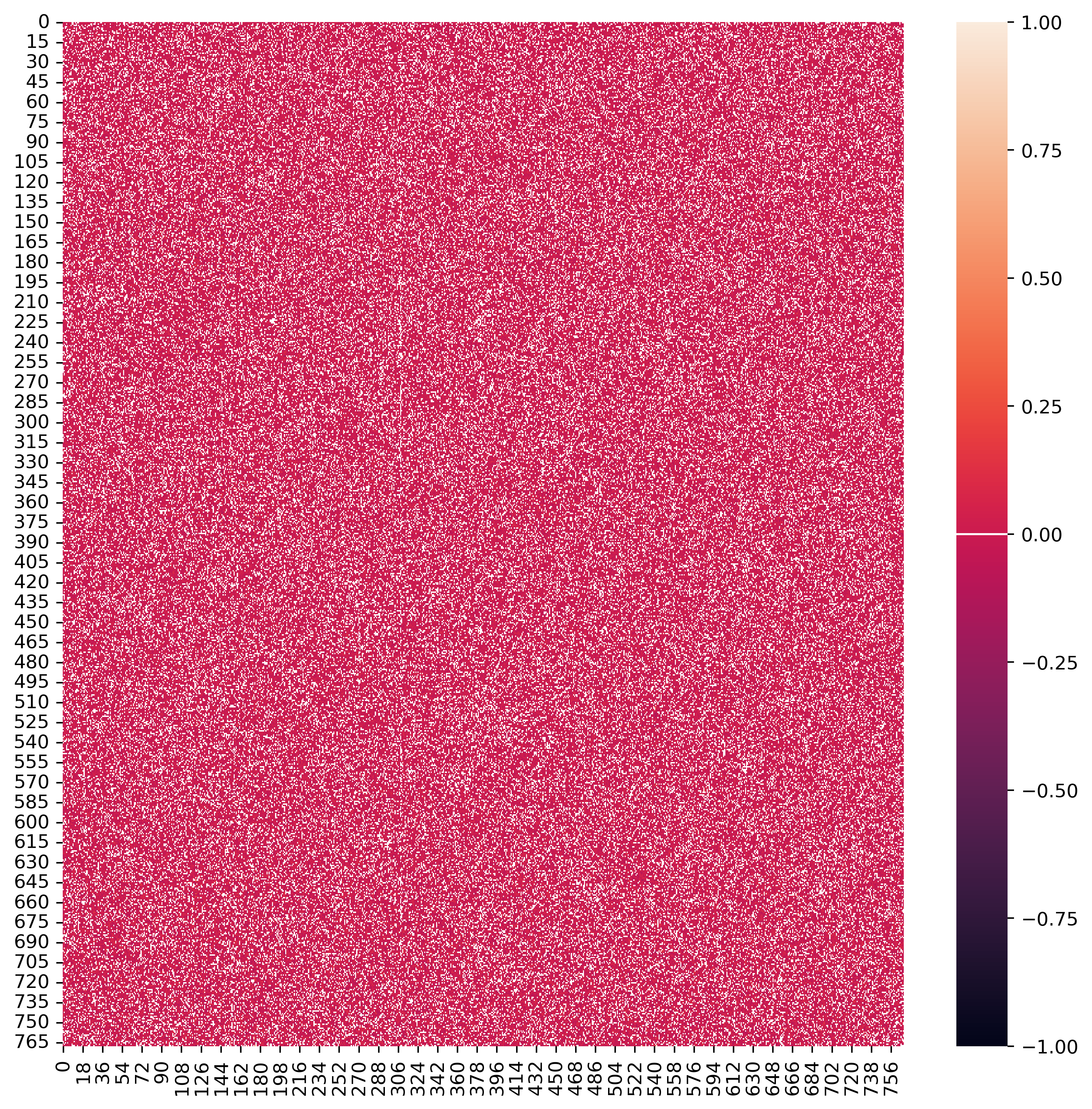
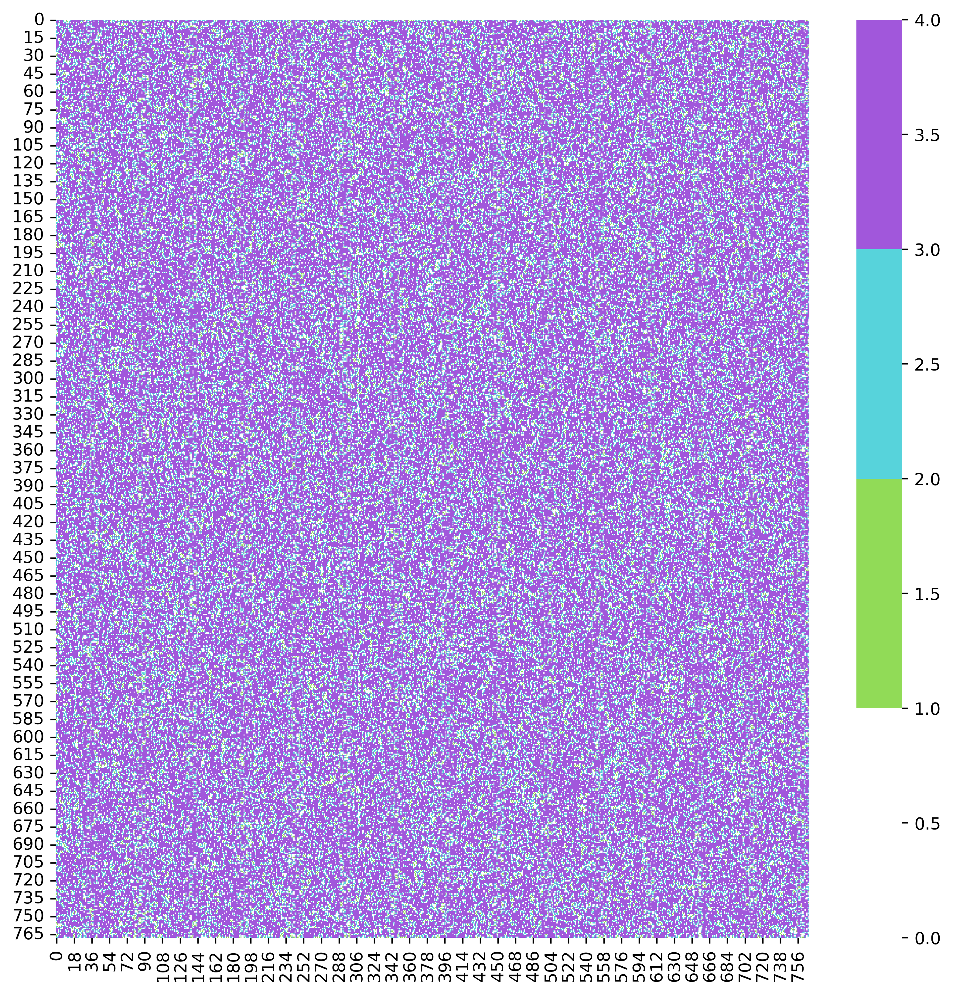
(a) Parameter reset 21.87%

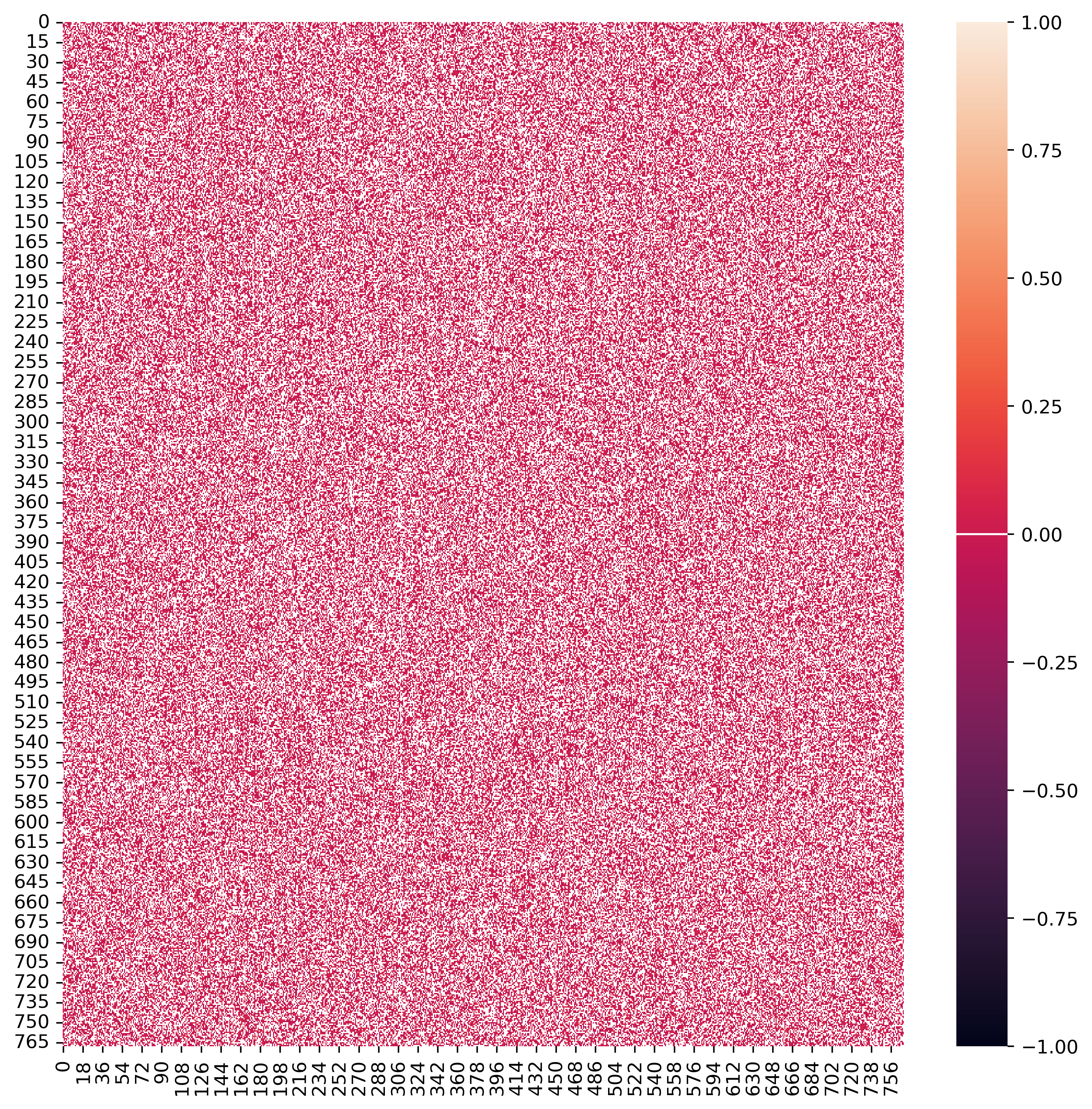
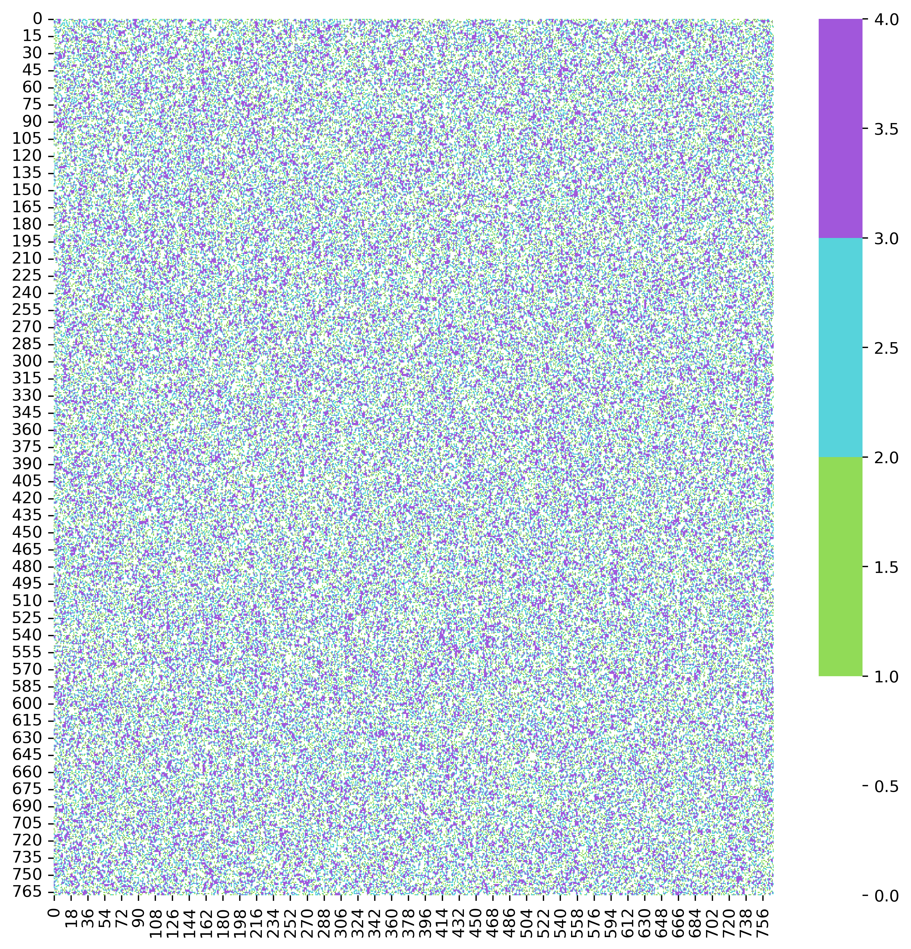
(b) Parameter reset 47.91%

(c) Parameter reset 73.95%

Figure 6: Visualization of the key attention matrix at layer 0 of a BERT model trained on the glue-sst2 dataset, utilizing KEN_viz. The left-hand figures depict the matrix after undergoing the KEN pruning stage, while the right-hand ones showcase the corresponding neighbor counts

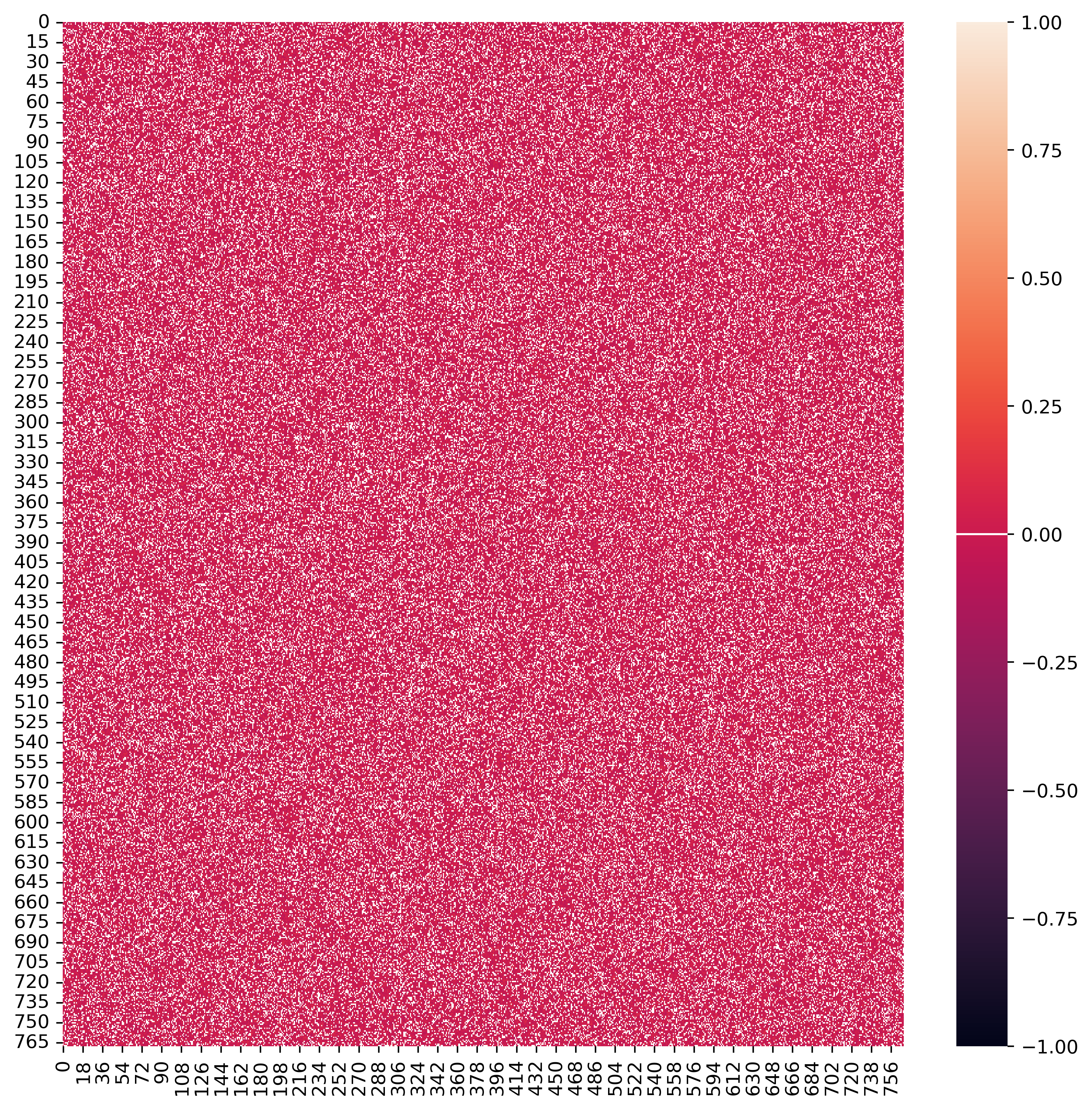
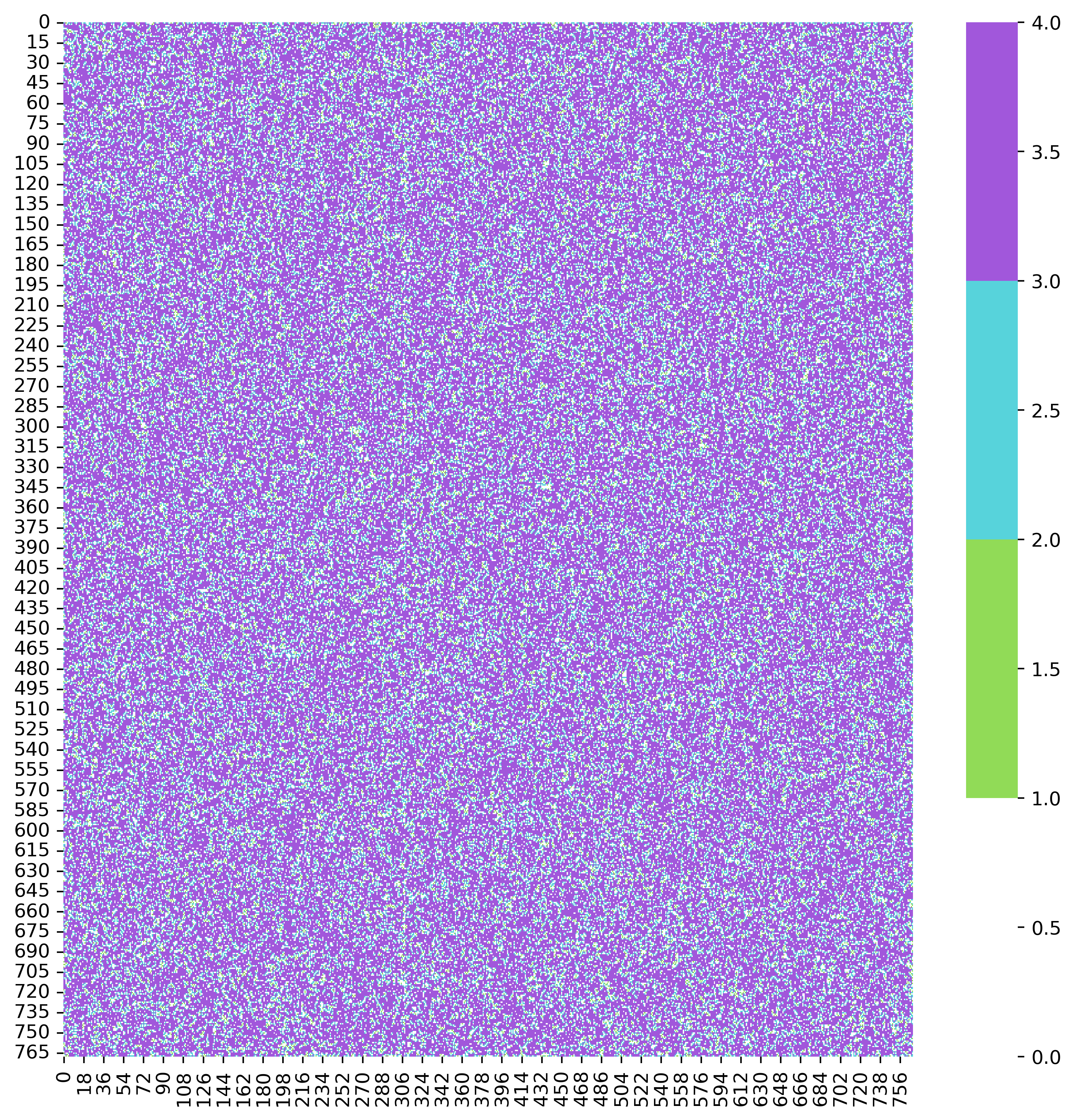
(a) Parameter reset 21.87%

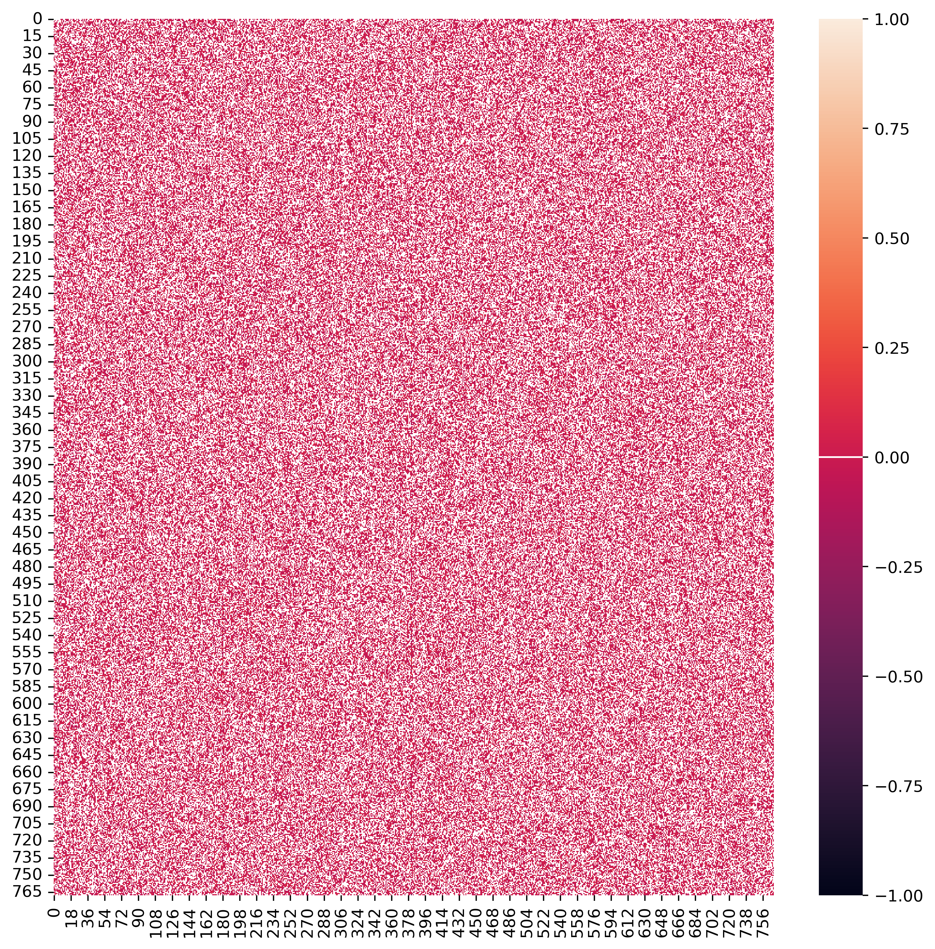
(b) Parameter reset 47.91%

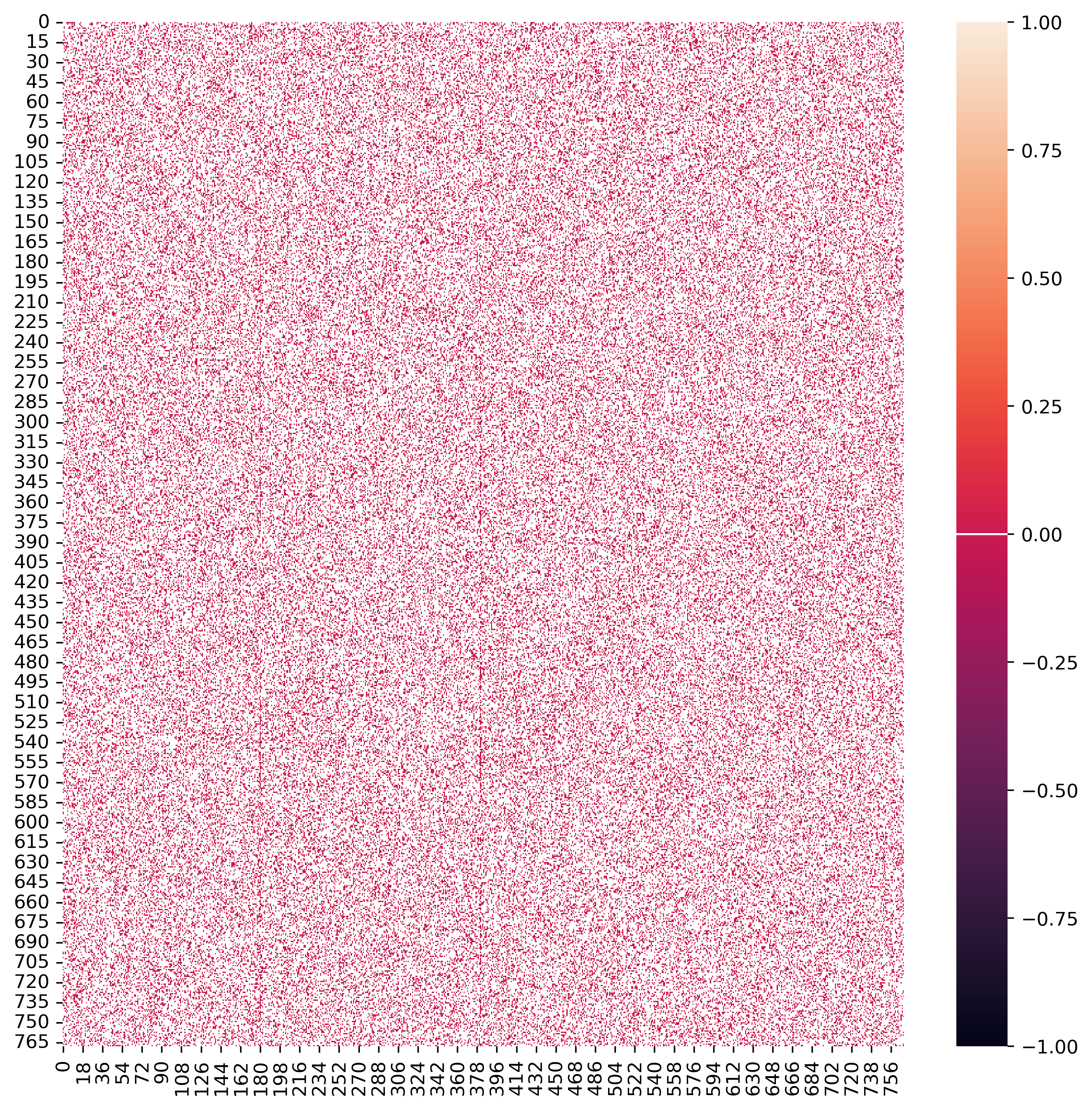
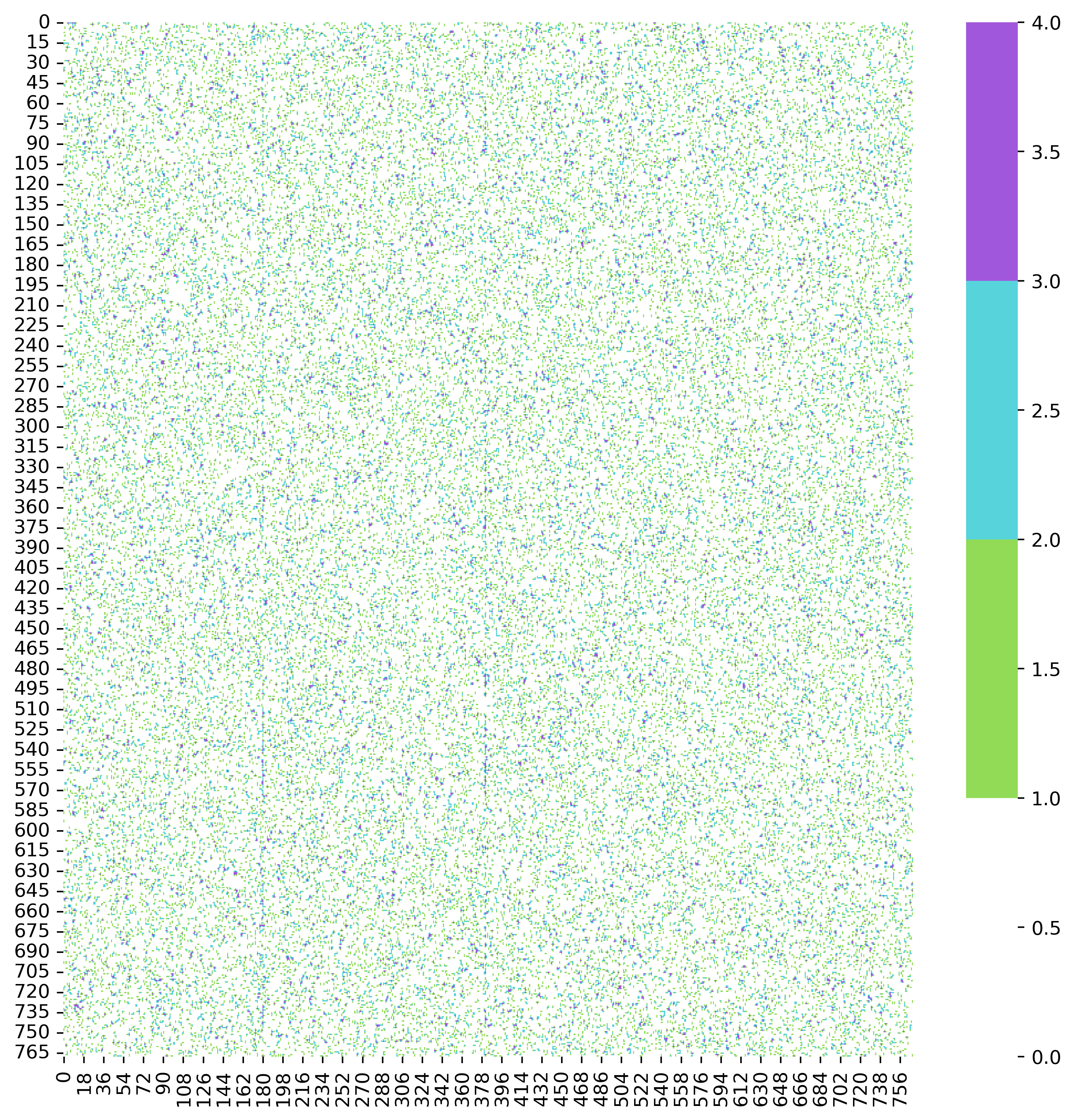
(c) Parameter reset 73.95%

Figure 7: Visualization of the key attention matrix at layer 12 of a BERT model trained on the glue-sst2 dataset, utilizing KEN_viz. The left-hand figures depict the matrix after undergoing the KEN pruning stage, while the right-hand ones showcase the corresponding neighbor counts

References

- Ba and Caruana (2014) Jimmy Ba and Rich Caruana. 2014. Do deep nets really need to be deep? Advances in neural information processing systems, 27.
- Barbieri et al. (2020) Francesco Barbieri, Jose Camacho-Collados, Luis Espinosa Anke, and Leonardo Neves. 2020. TweetEval: Unified benchmark and comparative evaluation for tweet classification. In Findings of the Association for Computational Linguistics: EMNLP 2020, pages 1644–1650, Online. Association for Computational Linguistics.
- Bastings et al. (2019) Jasmijn Bastings, Wilker Aziz, and Ivan Titov. 2019. Interpretable neural predictions with differentiable binary variables. arXiv preprint arXiv:1905.08160.
- Benbaki et al. (2023) Riade Benbaki, Wenyu Chen, Xiang Meng, Hussein Hazimeh, Natalia Ponomareva, Zhe Zhao, and Rahul Mazumder. 2023. Fast as chita: Neural network pruning with combinatorial optimization. arXiv preprint arXiv:2302.14623.
- Blalock et al. (2020) Davis Blalock, Jose Javier Gonzalez Ortiz, Jonathan Frankle, and John Guttag. 2020. What is the state of neural network pruning? Proceedings of machine learning and systems, 2:129–146.
- Chatterjee et al. (2019) Ankush Chatterjee, Kedhar Nath Narahari, Meghana Joshi, and Puneet Agrawal. 2019. SemEval-2019 task 3: EmoContext contextual emotion detection in text. In Proceedings of the 13th International Workshop on Semantic Evaluation, pages 39–48, Minneapolis, Minnesota, USA. Association for Computational Linguistics.
- Clark et al. (2020) Kevin Clark, Minh-Thang Luong, Quoc V Le, and Christopher D Manning. 2020. Electra: Pre-training text encoders as discriminators rather than generators. arXiv preprint arXiv:2003.10555.
- Cohan et al. (2019) Arman Cohan, Waleed Ammar, Madeleine van Zuylen, and Field Cady. 2019. Structural scaffolds for citation intent classification in scientific publications. In Proceedings of the 2019 Conference of the North American Chapter of the Association for Computational Linguistics: Human Language Technologies, Volume 1 (Long and Short Papers), pages 3586–3596, Minneapolis, Minnesota. Association for Computational Linguistics.
- Davidson et al. (2017) Thomas Davidson, Dana Warmsley, Michael Macy, and Ingmar Weber. 2017. Automated hate speech detection and the problem of offensive language. In Proceedings of the international AAAI conference on web and social media, volume 11, pages 512–515.
- de Gibert et al. (2018) Ona de Gibert, Naiara Perez, Aitor García-Pablos, and Montse Cuadros. 2018. Hate Speech Dataset from a White Supremacy Forum. In Proceedings of the 2nd Workshop on Abusive Language Online (ALW2), pages 11–20, Brussels, Belgium. Association for Computational Linguistics.
- Devlin et al. (2018) Jacob Devlin, Ming-Wei Chang, Kenton Lee, and Kristina Toutanova. 2018. Bert: Pre-training of deep bidirectional transformers for language understanding. arXiv preprint arXiv:1810.04805.
- Dong et al. (2017) Xin Dong, Shangyu Chen, and Sinno Pan. 2017. Learning to prune deep neural networks via layer-wise optimal brain surgeon. Advances in neural information processing systems, 30.
- Frankle and Carbin (2018) Jonathan Frankle and Michael Carbin. 2018. The lottery ticket hypothesis: Finding sparse, trainable neural networks. arXiv preprint arXiv:1803.03635.
- Gong et al. (2014) Yunchao Gong, Liu Liu, Ming Yang, and Lubomir Bourdev. 2014. Compressing deep convolutional networks using vector quantization. arXiv preprint arXiv:1412.6115.
- Gordon et al. (2020) Mitchell A Gordon, Kevin Duh, and Nicholas Andrews. 2020. Compressing bert: Studying the effects of weight pruning on transfer learning. arXiv preprint arXiv:2002.08307.
- Gulli (2005) Antonio Gulli. 2005. Ag’s corpus of news articles.
- Gurulingappa et al. (2012) Harsha Gurulingappa, Abdul Mateen Rajput, Angus Roberts, Juliane Fluck, Martin Hofmann-Apitius, and Luca Toldo. 2012. Development of a benchmark corpus to support the automatic extraction of drug-related adverse effects from medical case reports. Journal of Biomedical Informatics, 45(5):885 – 892. Text Mining and Natural Language Processing in Pharmacogenomics.
- Han et al. (2015) Song Han, Jeff Pool, John Tran, and William Dally. 2015. Learning both weights and connections for efficient neural network. Advances in neural information processing systems, 28.
- Hanson and Pratt (1988) Stephen Hanson and Lorien Pratt. 1988. Comparing biases for minimal network construction with back-propagation. Advances in neural information processing systems, 1.
- Hassibi and Stork (1992) Babak Hassibi and David Stork. 1992. Second order derivatives for network pruning: Optimal brain surgeon. Advances in neural information processing systems, 5.
- He et al. (2020) Pengcheng He, Xiaodong Liu, Jianfeng Gao, and Weizhu Chen. 2020. Deberta: Decoding-enhanced bert with disentangled attention. arXiv preprint arXiv:2006.03654.
- Hu et al. (2021) Edward J Hu, Yelong Shen, Phillip Wallis, Zeyuan Allen-Zhu, Yuanzhi Li, Shean Wang, Lu Wang, and Weizhu Chen. 2021. Lora: Low-rank adaptation of large language models. arXiv preprint arXiv:2106.09685.
- Huang et al. (2018) Gao Huang, Shichen Liu, Laurens Van der Maaten, and Kilian Q Weinberger. 2018. Condensenet: An efficient densenet using learned group convolutions. In Proceedings of the IEEE conference on computer vision and pattern recognition, pages 2752–2761.
- Janowsky (1989) Steven A Janowsky. 1989. Pruning versus clipping in neural networks. Physical Review A, 39(12):6600.
- Joulin et al. (2017) Armand Joulin, Moustapha Cissé, David Grangier, Hervé Jégou, et al. 2017. Efficient softmax approximation for gpus. In International conference on machine learning, pages 1302–1310. PMLR.
- Keung et al. (2020) Phillip Keung, Yichao Lu, György Szarvas, and Noah A. Smith. 2020. The multilingual amazon reviews corpus. In Proceedings of the 2020 Conference on Empirical Methods in Natural Language Processing.
- Kim and Rush (2016) Yoon Kim and Alexander M Rush. 2016. Sequence-level knowledge distillation. arXiv preprint arXiv:1606.07947.
- Lagunas et al. (2021) François Lagunas, Ella Charlaix, Victor Sanh, and Alexander M Rush. 2021. Block pruning for faster transformers. arXiv preprint arXiv:2109.04838.
- LeCun et al. (1989) Yann LeCun, John Denker, and Sara Solla. 1989. Optimal brain damage. Advances in neural information processing systems, 2.
- Li and Roth (2002) Xin Li and Dan Roth. 2002. Learning question classifiers. In COLING 2002: The 19th International Conference on Computational Linguistics.
- Maas et al. (2011) Andrew L. Maas, Raymond E. Daly, Peter T. Pham, Dan Huang, Andrew Y. Ng, and Christopher Potts. 2011. Learning word vectors for sentiment analysis. In Proceedings of the 49th Annual Meeting of the Association for Computational Linguistics: Human Language Technologies, pages 142–150, Portland, Oregon, USA. Association for Computational Linguistics.
- Malach et al. (2020) Eran Malach, Gilad Yehudai, Shai Shalev-Schwartz, and Ohad Shamir. 2020. Proving the lottery ticket hypothesis: Pruning is all you need. In International Conference on Machine Learning, pages 6682–6691. PMLR.
- Mozer and Smolensky (1989) Michael C Mozer and Paul Smolensky. 1989. Using relevance to reduce network size automatically. Connection Science, 1(1):3–16.
- Pang and Lee (2005) Bo Pang and Lillian Lee. 2005. Seeing stars: Exploiting class relationships for sentiment categorization with respect to rating scales. arXiv preprint cs/0506075.
- Sajjad et al. (2020) Hassan Sajjad, Fahim Dalvi, Nadir Durrani, and Preslav Nakov. 2020. Poor man’s bert: Smaller and faster transformer models. arXiv preprint arXiv:2004.03844, 2(2).
- Sanh et al. (2019) Victor Sanh, Lysandre Debut, Julien Chaumond, and Thomas Wolf. 2019. Distilbert, a distilled version of bert: smaller, faster, cheaper and lighter. arXiv preprint arXiv:1910.01108.
- Sanh et al. (2020) Victor Sanh, Thomas Wolf, and Alexander Rush. 2020. Movement pruning: Adaptive sparsity by fine-tuning. Advances in Neural Information Processing Systems, 33:20378–20389.
- Scott (2015) David W Scott. 2015. Multivariate density estimation: theory, practice, and visualization. John Wiley & Sons.
- Sheng and Uthus (2020) Emily Sheng and David Uthus. 2020. Investigating societal biases in a poetry composition system. In Proceedings of the Second Workshop on Gender Bias in Natural Language Processing, pages 93–106, Barcelona, Spain (Online). Association for Computational Linguistics.
- Singh and Alistarh (2020) Sidak Pal Singh and Dan Alistarh. 2020. Woodfisher: Efficient second-order approximation for neural network compression. Advances in Neural Information Processing Systems, 33:18098–18109.
- Socher et al. (2013) Richard Socher, Alex Perelygin, Jean Wu, Jason Chuang, Christopher D. Manning, Andrew Ng, and Christopher Potts. 2013. Recursive deep models for semantic compositionality over a sentiment treebank. In Proceedings of the 2013 Conference on Empirical Methods in Natural Language Processing, pages 1631–1642, Seattle, Washington, USA. Association for Computational Linguistics.
- Sun et al. (2020) Yu Sun, Shuohuan Wang, Yukun Li, Shikun Feng, Hao Tian, Hua Wu, and Haifeng Wang. 2020. Ernie 2.0: A continual pre-training framework for language understanding. In Proceedings of the AAAI conference on artificial intelligence, volume 34, pages 8968–8975.
- Sze et al. (2017) Vivienne Sze, Yu-Hsin Chen, Tien-Ju Yang, and Joel S Emer. 2017. Efficient processing of deep neural networks: A tutorial and survey. Proceedings of the IEEE, 105(12):2295–2329.
- Vaswani et al. (2017) Ashish Vaswani, Noam Shazeer, Niki Parmar, Jakob Uszkoreit, Llion Jones, Aidan N Gomez, Łukasz Kaiser, and Illia Polosukhin. 2017. Attention is all you need. Advances in neural information processing systems, 30.
- Wang et al. (2019) Ziheng Wang, Jeremy Wohlwend, and Tao Lei. 2019. Structured pruning of large language models. arXiv preprint arXiv:1910.04732.
- Workshop et al. (2022) BigScience Workshop, Teven Le Scao, Angela Fan, Christopher Akiki, Ellie Pavlick, Suzana Ilić, Daniel Hesslow, Roman Castagné, Alexandra Sasha Luccioni, François Yvon, et al. 2022. Bloom: A 176b-parameter open-access multilingual language model. arXiv preprint arXiv:2211.05100.
- Yang et al. (2017) Tien-Ju Yang, Yu-Hsin Chen, and Vivienne Sze. 2017. Designing energy-efficient convolutional neural networks using energy-aware pruning. In Proceedings of the IEEE conference on computer vision and pattern recognition, pages 5687–5695.
- Zhang et al. (2015) Xiang Zhang, Junbo Zhao, and Yann LeCun. 2015. Character-level convolutional networks for text classification. Advances in neural information processing systems, 28.
- Zhu et al. (2016) Chenzhuo Zhu, Song Han, Huizi Mao, and William J Dally. 2016. Trained ternary quantization. arXiv preprint arXiv:1612.01064.
- Zhu and Gupta (2017) Michael Zhu and Suyog Gupta. 2017. To prune, or not to prune: exploring the efficacy of pruning for model compression. arXiv preprint arXiv:1710.01878.