Boosting Long-Delayed Reinforcement Learning with
Auxiliary Short-Delayed Task

Abstract

Reinforcement learning is challenging in delayed scenarios, a common real-world situation where observations and interactions occur with delays. State-of-the-art (SOTA) state-augmentation techniques either suffer from the state-space explosion along with the delayed steps, or performance degeneration in stochastic environments. To address these challenges, our novel Auxiliary-Delayed Reinforcement Learning (AD-RL) leverages an auxiliary short-delayed task to accelerate the learning on a long-delayed task without compromising the performance in stochastic environments. Specifically, AD-RL learns the value function in the short-delayed task and then employs it with the bootstrapping and policy improvement techniques in the long-delayed task. We theoretically show that this can greatly reduce the sample complexity compared to directly learning on the original long-delayed task. On deterministic and stochastic benchmarks, our method remarkably outperforms the SOTAs in both sample efficiency and policy performance.

1 Introduction

Reinforcement learning (RL) has already shown its promising success in learning complex tasks such as Go (Silver et al., 2018), MOBA Game (Berner et al., 2019), and cyber-physics systems (Xu et al., 2021; Wang et al., 2023a, b; Zhan et al., 2023). Most of the above RL settings assume that the agent’s interaction with the environment is instantaneous, which means that the agent can always execute commands without delay and gather feedback from the environment right away. However, the persistent presence of delays in real-world applications significantly hampers agents’ efficiency, performance, and safety if not handled properly (e.g., introducing estimation error (Hwangbo et al., 2017) and losing reproducibility (Mahmood et al., 2018) in practical robotic tasks). Delay also needs to be considered in many stochastic settings such as financial market (Hasbrouck & Saar, 2013) and weather forecasting (Fathi et al., 2022). Thus, addressing delays in RL algorithms is crucial for their deployment in real-world timing-sensitive tasks.

Delays in RL can be primarily divided into three categories: observation-delay, action-delay, and reward-delay (Firoiu et al., 2018), depending on where the delay occurs. Among them, observation-delay receives considerable attention due to the application-wise generality and the technique-wise challenge: it has been proved to be a superset of action-delay (Katsikopoulos & Engelbrecht, 2003; Nath et al., 2021), and unlike well-studied reward-delay (Han et al., 2022; Kim & Lee, 2020), it disrupts the Markovian property of systems (i.e., the underlying dynamics depend on an unobserved state and the sequence of actions). In this work, we focus on non-anonymous and constant observation-delay under finite Markov Decision Process (MDP) setting, where the delay-step is known to the agent and always a constant (details in Section 3), as in most existing works (Schuitema et al., 2010; Nath et al., 2021; Chen et al., 2021).

Figure 4: Our AD-RL method introduces an adjoint short-delayed task, enhancing the original augment-based method (A-QL) in deterministic MDP (Fig. LABEL:fig:de_motivating_example) with delay $\Delta=10$, shown in Fig. LABEL:fig:de_aux_delay_impact. Whereas, in stochastic MDP (Fig. LABEL:fig:sto_motivating_example) with delay $\Delta=10$, a short auxiliary delay may lead to performance improvement (AD-QL(5)) or drop (AD-QL(0)) as shown in Fig. LABEL:fig:sto_aux_delay_impact. BPQL always uses a fixed $0$ auxiliary delay-step, equivalent to AD-QL(0) in these examples. Notably, the optimal auxiliary delay is irregular and task-specific, which we discussed in subsequent experiments in Section 6.

The promising augment-based approaches (Altman & Nain, 1992; Katsikopoulos & Engelbrecht, 2003) reform the delayed RL problem into an MDP by augmenting the latest observed state with a sequence of actions related to the delay-step, also known as the information state (Bertsekas, 2012). After retrieving the Markovian property, the augment-based methods adopt the classical RL method to solve the delayed task properly, such as augmented Q-learning (A-QL) (Nath et al., 2021). However, existing augment-based methods are plagued by the curse of dimensionality, shown by our toy examples in Fig. 4. Under a deterministic MDP setting (Fig. LABEL:fig:de_motivating_example), the original augmented state space grows exponentially with the delay-steps causing learning inefficiency. The variant of augment-based methods BPQL (Kim et al., 2023) approximates the value function based on the delay-free MDP to tackle the inefficiency, which unexpectedly results in excessive information loss. Consequently, it cannot properly handle stochastic tasks (Fig. LABEL:fig:sto_motivating_example).

To address the aforementioned challenges, we propose a novel technique named Auxiliary-Delayed RL (AD-RL). Our AD-RL is inspired by a key observation that an elaborate auxiliary short-delayed task carries much more accurate information than the delay-free task about the original long-delayed task, and it is still easy to learn. By introducing the notion of delayed belief to bridge an auxiliary short-delayed task and the original long-delayed task, we can learn the auxiliary-delayed value function and map it to the original one. The changeable auxiliary delay in our AD-RL has the ability to flexibly address the trade-off between the learning efficiency and approximation accuracy error in various MDPs. In toy examples (Fig. LABEL:fig:de_motivating_example and Fig. LABEL:fig:sto_motivating_example) with 10 delay-steps, we compare the performance of A-QL and AD-RL with 0 and 5 auxiliary delay steps respectively (AD-QL(0) and AD-QL(5)). Our AD-RL can not only remarkably enhance the learning efficiency (Fig. LABEL:fig:de_aux_delay_impact) but also possess the flexibility to capture more information under the stochastic setting (Fig. LABEL:fig:sto_aux_delay_impact). Notably, BPQL is a special variant of our AD-RL with the fixed 0 auxiliary delay, resulting in poor performance under the stochastic setting. In Section 4, we develop AD-DQN and AD-SAC, extending from Deep Q-Network and Soft Actor-Critic with our AD-RL framework respectively. Besides, we provide an in-depth theoretical analysis of learning efficiency, performance gap, and convergence in Section 5. In Section 6, we show superior efficacy of our method compared with the SOTA approaches on the different benchmarks. Our contributions can be summarized as follows:

• We address the sample inefficiency of the original augment-based approaches (denoted as A-RL) and excessive approximation error of the belief-based approaches by introducing AD-RL, which is more efficient with a short auxiliary-delayed task and achieves a theoretical similar performance with A-RL.

• Adapting the AD-RL framework, we devise AD-DQN and AD-SAC to handle discrete and continuous control tasks respectively.

• We analyze the superior sampling efficiency of AD-RL, the performance gap bound between AD-RL and A-RL, and provide the convergence guarantee of AD-RL.

• We empirically show notable improvements of AD-RL from policy performance and sampling efficiency aspects via comparing with existing SOTA methods in both deterministic and stochastic benchmarks.

2 Preliminaries

2.1 Delay-free RL

The delay-free RL problem is usually based on a Markov Decision Process (MDP), defined as a tuple $\langle\mathcal{S},\mathcal{A},\mathcal{P},\mathcal{R},\gamma,\rho\rangle$. An MDP consists of a state space $\mathcal{S}$, an action space $\mathcal{A}$, a probabilistic transition function $\mathcal{P}:\mathcal{S}\times\mathcal{A}\times\mathcal{S}\rightarrow[0,1]$, a reward function $\mathcal{R}:\mathcal{S}\times\mathcal{A}\rightarrow\mathbb{R}$, a discount factor $\gamma\in(0,1)$ and an initial state distribution $\rho$. At each time step $t$, based on the input state $s_{t}\in\mathcal{S}$ and the policy $\pi:\mathcal{S}\times\mathcal{A}\rightarrow[0,1]$, the agent has an action $a_{t}\sim\pi(\cdot|s_{t})$ where $a_{t}\in\mathcal{A}$, and then the MDP evolves to a new state $s_{t+1}\in\mathcal{S}$ based on the probabilistic transition function $\mathcal{P}$ and the agent receive a reward signal $r_{t}$ from reward function $\mathcal{R}(s_{t},a_{t})$. We use $d_{s_{0}}^{\pi}$ to denote the visited state distribution starting from $s_{0}$ based on policy $\pi$. The objective of the agent in an MDP is to find a policy that maximizes return over the horizon $H$. Given a state $s$, the value function of policy $\pi$ is defined as

$$V^{\pi}(s)=\mathop{\mathbb{E}}_{s_{t+1}\sim\mathcal{P}(\cdot|s_{t},a_{t})\atop a_{t}\sim\pi(\cdot|s_{t})}\left[\sum_{t=0}^{H}\gamma^{t}\mathcal{R}(s_{t},a_{t})\middle|s_{0}=s\right].$$

Similarly, given a state-action pair $(s,a)$, the Q-function of policy $\pi$ can be defined as

$$Q^{\pi}(s,a)=\mathop{\mathbb{E}}_{s_{t+1}\sim\mathcal{P}(\cdot|s_{t},a_{t})\atop a_{t}\sim\pi(\cdot|s_{t})}\left[\sum_{t=0}^{H}\gamma^{t}\mathcal{R}(s_{t},a_{t})\middle|{s_{0}=s\atop a_{0}=a}\right].$$

2.2 Deep Q-Network and Soft Actor-Critic

As the most classical off-policy RL method, Deep Q-Network (DQN) (Mnih et al., 2015) with the Q-function $Q_{\theta}:\mathcal{S}\times\mathcal{A}\rightarrow\mathbb{R}$ parameterized by $\theta$ conducts the temporal-difference (TD) learning based on the Bellman optimality equation. Given the transition data $(s_{t},a_{t},r_{t},s_{t+1})$, DQN updates the Q-function via minimizing TD error.

$$\nabla_{\theta}\left[\frac{1}{2}(Q_{\theta}(s_{t},a_{t})-\mathbb{Y})^{2}\right]$$

where $\mathbb{Y}=r_{t}+\gamma\max_{a_{t+1}}Q_{\theta}(s_{t+1},a_{t+1})$ is the TD target.

Based on the maximum entropy principle, Soft Actor-Critic (SAC) (Haarnoja et al., 2018a) provides a more stable actor-critic method by introducing a soft value function. Given transition data $(s_{t},a_{t},r_{t},s_{t+1})$, SAC conducts TD update for the critic using the soft TD target $\mathbb{Y}^{soft}$.

$$\mathbb{Y}^{soft}=r_{t}$$

$$+\gamma\mathop{\mathbb{E}}_{a_{t+1}\sim\pi_{\psi}(\cdot|s_{t+1})}\left[{Q_{\theta}}(s_{t+1},a_{t+1})-\log\pi_{\psi}(a_{t+1}|s_{t+1})\right]$$

where $\pi_{\psi}$ is the policy function parameterized by $\psi$. For the policy $\pi_{\psi}$, it can be optimized by the gradient update:

$$\nabla_{\psi}\mathop{\mathbb{E}}_{\hat{a}\sim\pi_{\psi}(\cdot|s_{t})}\left[\log\pi_{\psi}(\hat{a}|s_{t})-Q_{\theta}(s_{t},\hat{a})\right]$$

3 Problem Setting

We assume that delay-free MDP is endowed with a constant delay variable $\Delta\in\mathbb{N}$. In this setting, the state of environment $s_{t}$ is only observed by the agent at a later timestep ${t+\Delta}$. In other words, the real state of the environment is $s_{t}$, but the agent’s observation is $s_{t-\Delta}$. To retrieve the Markov property in this Delayed MDP (DMDP) (Altman & Nain, 1992; Katsikopoulos & Engelbrecht, 2003), we need to augment the state space $\mathcal{X}=\mathcal{S}\times\mathcal{A}^{\Delta}$, where $\mathcal{A}^{\Delta}$ stands for actions in delay time steps. An augmented state $x_{t}=(s_{t-\Delta},a_{t-\Delta},\ldots,a_{t-1})\in\mathcal{X}$ is composed with the latest observed state $s_{t-\Delta}$ and actions taken in last $\Delta$ time steps $(a_{t-\Delta},\ldots,a_{t-1})$. Thus, with consideration of the delay into the dynamics, we can formulate a new MDP dynamic called Constant Delayed MDP (CDMDP), $\langle\mathcal{X},\mathcal{A},\mathcal{P}_{\Delta},\mathcal{R}_{\Delta},\gamma,\rho_{\Delta}\rangle$, where $\mathcal{X}$ is defined above, $\mathcal{A}$ stands for the action-space. $\mathcal{P}_{\Delta}$ is the delayed probabilistic transition function defined below.

$$\mathcal{P}_{\Delta}(x_{t+1}|x_{t},a_{t})=$$

$$\mathcal{P}(s_{t-\Delta+1}|s_{t-\Delta},a_{t-\Delta})\delta_{a_{t}}(a^{\prime}_{t})\Pi_{i=1}^{\Delta-1}\delta_{a_{t-i}}(a^{\prime}_{t-i})$$

where $\delta$ is the Dirac distribution. We also have a new delayed reward function $\mathcal{R}_{\Delta}$ defined as follow.

$$\mathcal{R}_{\Delta}(x_{t},a_{t})=\mathop{\mathbb{E}}_{s_{t}\sim b(\cdot|x_{t})}[\mathcal{R}(s_{t},a_{t})]$$

Correspondingly, the initial state distribution is represented as $\rho_{\Delta}=\rho\Pi_{i=1}^{\Delta}\delta_{a_{-i}}$, where $b(s_{t}|x_{t})$ is called belief defined as follows.

$$b(s_{t}|x_{t})=$$ (1)

$$\int_{\mathcal{S}^{\Delta}}\Pi_{i=0}^{\Delta-1}\mathcal{P}(s_{t-\Delta+i+1}|s_{t-\Delta+i},a_{t-\Delta+i})\mathrm{d}{s_{t-\Delta+i+1}}$$

The idea is to infuse delayed state information $s_{t-\Delta}$ to $s_{t}$ into the augmented state $x_{t}$ (Gangwani et al., 2020).

In this work, we assume the MDPs, policies and Q-functions satisfy the following Lipschitz Continuity (LC) property, where Euclidean distance is adopted in a deterministic space (e.g., $d_{\mathcal{S}}$ for state space $\mathcal{S}$, $d_{\mathcal{A}}$ for action space $\mathcal{A}$ and $d_{\mathcal{R}}$ for reward space $\mathcal{R}$), and $L1$-Wasserstein distance (Villani et al., 2009), denoted as $W_{1}$, is used in a probabilistic space (e.g., transition space $\mathcal{P}$ and policy space $\Pi$) respectively.

Definition 3.1 (Lipschitz Continuous MDP (Rachelson & Lagoudakis, 2010)).

An MDP $\langle\mathcal{S},\mathcal{A},\mathcal{P},\mathcal{R},\gamma,\rho\rangle$ is $(L_{\mathcal{P}},L_{\mathcal{R}})$-LC, if $\forall(s_{1},a_{1}),(s_{2},a_{2})\in\mathcal{S}\times\mathcal{A}$

$$W_{1}(\mathcal{P}(\cdot|s_{1},a_{1})||\mathcal{P}(\cdot|s_{2},a_{2}))\leq L_{\mathcal{P}}(d_{\mathcal{S}}(s_{1},s_{2})+d_{\mathcal{A}}(a_{1},a_{2}))$$

$$d_{\mathcal{R}}(\mathcal{R}(s_{1},a_{1})-\mathcal{R}(s_{2},a_{2}))\leq L_{\mathcal{R}}(d_{\mathcal{S}}(s_{1},s_{2})+d_{\mathcal{A}}(a_{1},a_{2}))$$

Definition 3.2 (Lipschitz Continuous Policy (Rachelson & Lagoudakis, 2010)).

A stationary markovian policy $\pi$ is $L_{\pi}$-LC, if $\forall s_{1},s_{2}\in\mathcal{S}$, we have

$$W_{1}(\pi(\cdot|s_{1})||\pi(\cdot|s_{2}))\leq L_{\pi}d_{\mathcal{S}}(s_{1},s_{2})$$

Definition 3.3 (Lipschitz Continuous Q-function (Rachelson & Lagoudakis, 2010)).

Given $(L_{\mathcal{P}},L_{\mathcal{R}})$-LC MDP and $L_{\pi}$-LC policy $\pi$, such that $\gamma L_{P}(1+L_{\pi})<1$ where $\gamma$ is the discount factor of MDP, then Q-function $Q^{\pi}$ is $L_{Q}$-LC with $L_{Q}=\frac{L_{R}}{1-\gamma L_{P}(1+L_{\pi})}$.

Note that is a mild assumption commonly used in RL literature (Rachelson & Lagoudakis, 2010; Liotet et al., 2022).

4 Our Approach: Auxiliary-Delayed RL

In this section, we introduce our AD-RL framework to address the sample inefficiency of the original augment-based approach and illustrate the underlying relation between learning the original delayed task and the auxiliary one in Section 4.1. Then we extend the AD-RL framework to the practical algorithms in Section 4.2 and Section 4.3.

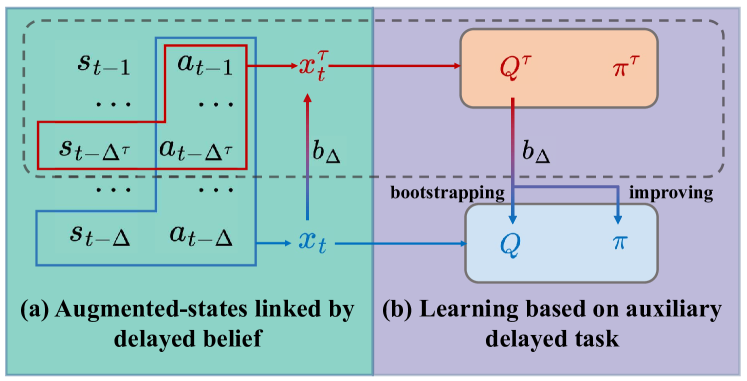
Figure 5: The overview of AD-RL framework. Compared with the conventional augment-based method, AD-RL additionally introduces the auxiliary-delayed task shown in the dashline box.

4.1 Auxiliary-Delayed Reinforcement Learning

Instead of learning on the original augmented state space $\mathcal{X}$ with delay-step $\Delta$, we introduce a corresponding auxiliary-delayed task with the shorter delay-step $\Delta^{\tau}$($\Delta^{\tau}$$<$$\Delta$) and, accordingly, a much smaller augmented state space $\mathcal{X}^{\tau}$. Sharing a similar idea as belief function $b$ in Eq. (LABEL:eq:belief_function), $\mathcal{X}$ and $\mathcal{X}^{\tau}$ can be bridged by a delayed belief function $b_{\Delta}$ as:

$$b_{\Delta}({\color[rgb]{1,0,0}x^{\tau}_{t}}|{\color[rgb]{0,0,1}x_{t}})=$$ (2)

$$\int_{\mathcal{S}^{\Delta}}\Pi_{i=0}^{\Delta-\Delta^{\tau}-1}\mathcal{P}(s_{t-\Delta+i+1}|s_{t-\Delta+i},a_{t-\Delta+i})\mathrm{d}{s_{t-\Delta+i+1}}$$

where ${\color[rgb]{0,0,1}x_{t}}=(s_{t-\Delta},a_{t-\Delta},\ldots,a_{t-1})\in{\color[rgb]{0,0,1}\mathcal{X}}$ and ${\color[rgb]{1,0,0}x^{\tau}_{t}}=(s_{t-{\Delta^{\tau}}},a_{t-\Delta^{\tau}},\ldots,a_{t-1})\in{\color[rgb]{1,0,0}\mathcal{X}^{\tau}}$. As shown in the Fig. 5 (a), both $x_{t}$ and $x^{\tau}_{t}$ share the sub-sequence $(a_{t-{\Delta^{\tau}}},\ldots,a_{t-1})$ of $\mathcal{A}^{\Delta}$. Besides, in the original MDP setting, transitioning from the state $s_{t-{\Delta}}$ to the state $s_{t-{\Delta^{\tau}}}$ can be accomplished by applying the action sub-sequence $(a_{t-{\Delta}},\ldots,a_{t-{\Delta^{\tau}}+1})$.

Remark 4.1 (Implicit Delayed Belief).

Practically, we do not need to learn the delayed belief $b_{\Delta}$ explicitly. As in the CDMDP, every state will be observed by the agent eventually. In other words, given an entire trajectory collected by the agent, we can create the synthetic augmented state with any required delay-step.

With $b_{\Delta}$ we can transform learning the original $\Delta$-delayed task into learning the auxiliary $\Delta^{\tau}$-delayed task which is much easier to learn for a much smaller augmented state space. As shown in Fig. 5 (b), we can use the easier-to-learn auxiliary Q-function $Q^{\tau}$ to help bootstrapping the Q-function $Q$ or improving the policy $\pi$. The specific algorithms will be proposed in the next sections. In this way, we can significantly improve the learning efficiency of the $\Delta$-delayed task, and a more rigorous proof will be presented in Section 5.

As a highly flexible delayed RL framework (Algorithm 1), our AD-RL can be naturally embedded in most of the existing RL methods to serve different task specifications. In this paper, we specifically develop two practical algorithms AD-DQN and AD-SAC based on DQN (Mnih et al., 2015) and SAC (Haarnoja et al., 2018a) to tackle discrete and continuous control tasks respectively.

Remark 4.2.

BPQL (Kim et al., 2023) can be seen as a special case of our AD-RL via setting the auxiliary delay to fixed zero (i.e., $\Delta^{\tau}$ $=0$). However, the excessive loss of information might lead to poor performance in stochastic MDP in Fig. LABEL:fig:sto_aux_delay_impact. We provide more experimental results about this in Section 6.

Algorithm 1 Auxiliary-Delayed RL Framework

  Input: $Q$, $\pi$ for $\Delta$ delay-step; $Q^{\tau}$, $\pi^{\tau}$ for $\Delta^{\tau}$ delay-step

  for each update step do

     # Learning $\Delta^{\tau}$-delayed task

     Updating $Q^{\tau}$, $\pi^{\tau}$ by a given delayed RL method

     # Learning $\Delta$-delayed task based on $Q^{\tau}$

     Bootstrapping $Q$ based on $Q^{\tau}$ via Eq. (3) $\#$ discrete

     Improving $\pi$ based on $Q^{\tau}$ via Eq. (5)$\#$ continuous

  end for

  Output: $Q$, $\pi$

4.2 Discrete Control: from AD-VI to AD-DQN

Before developing the practical algorithm: AD-DQN, we first have to derive AD-VI, the AD-RL version of value iteration (VI) (Sutton & Barto, 2018). In the tabular setting, AD-VI maintains two Q-functions $Q$ and $Q^{\tau}$ for the original delayed task($\Delta$) and the auxiliary-delayed task($\Delta^{\tau}$), respectively. Different from $Q^{\tau}$ updated by the original Bellman operator, we update $Q$ by applying the auxiliary-delayed Bellman operator $\mathcal{T}$ as follow:

$$\mathcal{T}{\color[rgb]{0,0,1}Q}({\color[rgb]{0,0,1}x_{t}},a_{t})\triangleq{\color[rgb]{0,0,1}\mathcal{R}_{\Delta}}({\color[rgb]{0,0,1}x_{t}},a_{t})$$ (3)

$$+\gamma\mathop{\mathbb{E}}_{{\color[rgb]{1,0,0}x^{\tau}_{t+1}}\sim b_{\Delta}(\cdot|{\color[rgb]{0,0,1}x_{t+1}})\atop{\color[rgb]{0,0,1}x_{t+1}}\sim\mathcal{P}_{\Delta}(\cdot|{\color[rgb]{0,0,1}x_{t}},a_{t})}\left[{\color[rgb]{1,0,0}Q^{\tau}}({\color[rgb]{1,0,0}x^{\tau}_{t+1}},{\mathop{\arg\max}_{a_{t+1}}}{\color[rgb]{0,0,1}Q}({\color[rgb]{0,0,1}x_{t+1}},a_{t+1}))\right]$$

Then AD-DQN can be extended from AD-VI naturally via approximating the Q-functions by the parameterized functions (e.g., neural networks). The implementation details of AD-DQN are presented in Appendix A.

4.3 Continuous Control: from AD-SPI to AD-SAC

Similarly, before AD-SAC, we begin with deriving AD-SPI, soft policy iteration (SPI) (Haarnoja et al., 2018a) in the context of our AD-RL. AD-SPI also alternates between two steps: policy evaluation and policy improvement. In policy evaluation, we evaluate the policy $\pi$ via iteratively applying the auxiliary-delayed soft Bellman operator $\mathcal{T}^{\pi}$ as follow:

$$\mathcal{T}^{\pi}{\color[rgb]{0,0,1}Q(x_{t},{\color[rgb]{0,0,0}a_{t}})}\triangleq{\color[rgb]{0,0,1}\mathcal{R}_{\Delta}}({\color[rgb]{0,0,1}x_{t}},a_{t})$$ (4)

$$+\gamma\mathop{\mathbb{E}}_{\begin{subarray}{c}{\color[rgb]{0,0,1}a_{t+1}\sim\pi(\cdot|x_{t+1})}\\ {\color[rgb]{1,0,0}x^{\tau}_{t+1}}\sim b_{\Delta}(\cdot|{\color[rgb]{0,0,1}x_{t+1}})\\ {\color[rgb]{0,0,1}x_{t+1}}\sim\mathcal{P}_{\Delta}(\cdot|{\color[rgb]{0,0,1}x_{t}},a_{t})\end{subarray}}\left[{\color[rgb]{1,0,0}Q^{\tau}(x^{\tau}_{t+1}},{\color[rgb]{0,0,1}a_{t+1}})-\log{\color[rgb]{0,0,1}\pi(a_{t+1}|x_{t+1})}\right]$$

where $Q^{\tau}$ is updated by the original soft Bellman operator (Haarnoja et al., 2018a). In policy improvement, we will update the policy $\pi$ based on $Q^{\tau}$ instead of $Q$ as follow:

$${\color[rgb]{0,0,1}\pi_{new}}=$$ (5)

$${\arg\min}_{{\color[rgb]{0,0,1}\pi^{\prime}\in\Pi}}\text{KL}\left({\color[rgb]{0,0,1}\pi^{\prime}(\cdot|x_{t})}\middle|\middle|\frac{\exp(\mathop{\mathbb{E}}_{{\color[rgb]{1,0,0}x^{\tau}_{t}}\sim b_{\Delta}(\cdot|{\color[rgb]{0,0,1}x_{t}})}[{\color[rgb]{1,0,0}Q^{\tau}(x^{\tau}_{t},\cdot)}])}{{\color[rgb]{1,0,0}Z(x^{\tau}_{t},\cdot)}}\right)$$

where $\Pi$ is the set of policies for tractable learning, KL is the Kullback-Leibler divergence and $Z$ is the term for normalizing the distribution. Functions approximations of the Q-functions ($Q$ and $Q^{\tau}$) and policies ($\pi$ and $\pi^{\tau}$) bring us AD-SAC, the practical algorithm for continuous control task. In AD-SAC, the policy $\pi_{\psi}$ parameterized by $\psi$ is updated by gradient with

$$\triangledown_{\psi}\mathop{\mathbb{E}}_{{\color[rgb]{0,0,1}\hat{a}\sim\pi_{\psi}(\cdot|x_{t})}\atop{\color[rgb]{1,0,0}x^{\tau}_{t}}\sim b_{\Delta}(\cdot|{\color[rgb]{0,0,1}x_{t}})}\left[\log{{\color[rgb]{0,0,1}\pi_{\psi}(\hat{a}|x_{t})}}-{{\color[rgb]{1,0,0}Q^{\tau}(x^{\tau}_{t}}},{{\color[rgb]{0,0,1}\hat{a}}})\right]$$ (6)

In addition, we further improve AD-SAC with multi-step value estimation (Sutton & Barto, 2018; Bouteiller et al., 2020) for accelerating learning. The implementation details of AD-SAC are presented in Appendix A.

5 Theoretical Analysis

In this section, we first discuss why our AD-RL has better sample efficiency in Section 5.1, then analyse that the performance gap between optimal auxiliary-delayed value function and optimal delayed value function in Section 5.2, and finally derive the convergence guarantee of our AD-RL in Section 5.3.

5.1 Sample Efficiency Analysis

Though it is hard to directly derive a formal conclusion on the sample efficiency of AD-RL, as the learning process is correlated to two different learning tasks at the same time, some existing works (Even-Dar et al., 2003; Azar et al., 2011) related to sample complexity provide insight into why our method has better sample efficiency. The sample complexity of the optimized Q-learning is $\mathcal{O}\left(\frac{\log(|\mathcal{S}||\mathcal{A}|)}{\epsilon^{2.5}(1-\gamma)^{5}}\right)$ (Azar et al., 2011), which shows the amount of samples are required for Q-learning to guarantee an $\epsilon$-optimal Q-function with high confidence. We can conclude that the sample complexity of augmented Q-learning in the augmented state space with delay-step $\Delta$ is $\mathcal{O}\left(\frac{\log(|\mathcal{S}||\mathcal{A}|^{\Delta+1})}{\epsilon^{2.5}(1-\gamma)^{5}}\right)$. Then our AD-RL makes bootstrapping in the auxiliary $\Delta^{\tau}$-augmented state-space instead of the original $\Delta$-augmented state-space, the sample efficiency is improved by $\mathcal{O}(|\mathcal{A}|^{{\color[rgb]{0,0,1}\Delta}-{\color[rgb]{1,0,0}\Delta_{\tau}}})$.

5.2 Performance Gap

While acknowledging that bootstrapping in a smaller augmented state space combined with delayed belief might lead to sub-optimal performance, we demonstrate in this section that this degradation can be effectively bounded. We start by deriving the Lemma 5.1, unifying performance gap between policies ($\pi$ and $\pi^{\tau}$) on the same auxiliary-delayed state space $\mathcal{X}^{\tau}$. Then, we derive the bounds on the performance gap through the difference of policies in Theorem 5.2. Next, we extend this bound to get the bound on Q-functions of different state spaces in Theorem 5.3. Finally, we show that the bound on optimal Q-functions will become nominal under the deterministic MDP setting.

Following the similar proof sketch with (Kakade & Langford, 2002; Liotet et al., 2022), we give the general delayed policies performance difference lemma as below.

Lemma 5.1 (General Delayed Performance Difference, see Appendix B.2 for proof).

For policies $\pi^{\tau}$ and $\pi$, with delay-steps $\Delta^{\tau}$ $<$ $\Delta$. Given any $x_{t}$ $\in$ $\mathcal{X}$, the performance difference is denoted as $I$($x_{t}$)

$$I({\color[rgb]{0,0,1}x_{t}}) =\mathop{\mathbb{E}}_{{\color[rgb]{1,0,0}x^{\tau}_{t}}\sim b_{\Delta}(\cdot|{\color[rgb]{0,0,1}x_{t}})}\left[{\color[rgb]{1,0,0}V^{\tau}(x^{\tau}_{t})}\right]-{\color[rgb]{0,0,1}V(x_{t})}$$

$$=\frac{1}{1-\gamma}\mathop{\mathbb{E}}_{\begin{subarray}{c}{\color[rgb]{1,0,0}\hat{x}^{\tau}}\sim b_{\Delta}(\cdot|{\color[rgb]{0,0,1}\hat{x}})\\ {\color[rgb]{0,0,1}a\sim\pi(\cdot|\hat{x})}\\ {\color[rgb]{0,0,1}\hat{x}\sim d_{x_{t}}^{\pi}}\end{subarray}}\left[{\color[rgb]{1,0,0}V^{\tau}(\hat{x}^{\tau})}-{\color[rgb]{1,0,0}Q^{\tau}}({\color[rgb]{1,0,0}\hat{x}^{\tau}},{\color[rgb]{0,0,1}a})\right]$$

Lemma 5.1 tells us that the performance difference $I$ between policies ($\pi$ and $\pi^{\tau}$) can be measured by the corresponding value functions ($V$ and $V^{\tau}$) sitting on different augmented state spaces ($\mathcal{X}$ and $\mathcal{X}^{\tau}$). Since the connection of $\mathcal{X}$ and $\mathcal{X}^{\tau}$ can be specified by the delayed belief $b_{\Delta}$, we can unify the expressions on $\mathcal{X}^{\tau}$ to measure the performance gap, using the auxiliary value functions ($V^{\tau}$ and $Q^{\tau}$). Assuming $Q^{\tau}$ is $L_{Q}$-LC (Definition 3.3), we can show that this performance difference between policies ($\pi$ and $\pi^{\tau}$) can be bounded by the $L_{1}$-Wassestein distance between them as followed Theorem 5.2.

Theorem 5.2 (Delayed Performance Difference Bound, proof in Appendix B.3).

For policies $\pi^{\tau}$ and $\pi$, with $\Delta^{\tau}$ $<$ $\Delta$. Given any $x_{t}$ $\in$ $\mathcal{X}$, if $Q^{\tau}$ is $L_{Q}$-LC, the performance difference between policies can be bounded as follow

$$\mathop{\mathbb{E}}_{{\color[rgb]{1,0,0}x^{\tau}_{t}}\sim b_{\Delta}(\cdot|{\color[rgb]{0,0,1}x_{t}})\atop{\color[rgb]{0,0,1}a_{t}\sim\pi(\cdot|x_{t})}}\left[{\color[rgb]{1,0,0}V^{\tau}(x^{\tau}_{t})}-{\color[rgb]{1,0,0}Q^{\tau}}({\color[rgb]{1,0,0}x^{\tau}_{t}},{\color[rgb]{0,0,1}a_{t}})\right]$$

$$\leq L_{Q}\mathop{\mathbb{E}}_{{\color[rgb]{1,0,0}x^{\tau}_{t}}\sim b_{\Delta}(\cdot|{\color[rgb]{0,0,1}x_{t}})}\left[{\mathcal{W}_{1}({\color[rgb]{1,0,0}\pi^{\tau}(\cdot|x^{\tau}_{t})}}||{\color[rgb]{0,0,1}\pi(\cdot|x_{t})})\right]$$

Combining Lemma 5.1 and Theorem 5.2, we can extend the bound on state-values ($V$ and $V^{\tau}$) to the bound on Q-values ($Q$ and $Q^{\tau}$) and optimal Q-values ($Q_{(*)}$ and $Q^{\tau}_{(*)}$) by the $L_{1}$-Wassestein distance of the corresponding policies ($\pi$ and $\pi^{\tau}$) and optimal policies ($\pi_{(*)}$ and $\pi^{\tau}_{(*)}$), respectively.

Theorem 5.3 (Delayed Q-value Difference Bound, proof in Appendix B.4).

For policies $\pi$ and $\pi^{\tau}$, with $\Delta^{\tau}$ $<$ $\Delta$. Given any $x_{t}$ $\in$ $\mathcal{X}$, if $Q^{\tau}$ is $L_{Q}$-LC, the corresponding Q-value difference can be bounded as follow

$$\mathop{\mathbb{E}}_{{\color[rgb]{0,0,1}a_{t}\sim\pi(\cdot|x_{t})}\atop{\color[rgb]{1,0,0}x^{\tau}_{t}}\sim b_{\Delta}(\cdot|{\color[rgb]{0,0,1}x_{t}})}\left[{\color[rgb]{1,0,0}Q^{\tau}}({\color[rgb]{1,0,0}x^{\tau}_{t}},{\color[rgb]{0,0,1}a_{t}})-{\color[rgb]{0,0,1}Q(x_{t},a_{t})}\right]$$

$$\leq\frac{\gamma L_{Q}}{1-\gamma}\mathop{\mathbb{E}}_{\begin{subarray}{c}{\color[rgb]{1,0,0}\hat{x}^{\tau}}\sim b_{\Delta}(\cdot|{\color[rgb]{0,0,1}\hat{x}})\\ {\color[rgb]{0,0,1}\hat{x}\sim d_{x_{t+1}}^{\pi}}\\ {\color[rgb]{0,0,1}x_{t+1}\sim\mathcal{P}_{\Delta}(\cdot|x_{t},a_{t})}\\ {\color[rgb]{0,0,1}a_{t}\sim\pi(\cdot|x_{t})}\end{subarray}}\left[\mathcal{W}_{1}({\color[rgb]{1,0,0}\pi^{\tau}(\cdot|\hat{x}^{\tau})}||{\color[rgb]{0,0,1}\pi(\cdot|\hat{x})})\right]$$

Specially, for optimal policies $\pi_{(*)}$ and $\pi^{\tau}_{(*)}$, if $Q^{\tau}_{(*)}$ is $L_{Q}$-LC, the corresponding optimal Q-value difference can be bounded as follow

$$\left|\left|\mathop{\mathbb{E}}_{{\color[rgb]{1,0,0}x^{\tau}_{t}}\sim b_{\Delta}(\cdot|{\color[rgb]{0,0,1}x_{t}})}\left[{\color[rgb]{1,0,0}Q^{\tau}_{(*)}({\color[rgb]{1,0,0}x^{\tau}_{t}}},a_{t})\right]-{\color[rgb]{0,0,1}Q_{(*)}(x_{t}},a_{t})\right|\right|_{\infty}$$

$$\leq\frac{\gamma^{2}L_{Q}}{(1-\gamma)^{2}}\mathop{\mathbb{E}}_{\begin{subarray}{c}{\color[rgb]{1,0,0}\hat{x}^{\tau}}\sim b_{\Delta}(\cdot|{\color[rgb]{0,0,1}\hat{x}})\\ {\color[rgb]{0,0,1}\hat{x}\sim d_{x_{t+1}}^{\pi}}\\ {\color[rgb]{0,0,1}x_{t+1}\sim\mathcal{P}_{\Delta}(\cdot|x_{t},a_{t})}\\ {\color[rgb]{0,0,1}a_{t}\sim\pi_{(*)}(\cdot|x_{t})}\end{subarray}}\left[\mathcal{W}_{1}\left({\color[rgb]{1,0,0}\pi^{\tau}_{(*)}(\cdot|\hat{x}^{\tau})}\middle|\middle|{\color[rgb]{0,0,1}\pi_{(*)}(\cdot|\hat{x})}\right)\right]$$

The results provided in Theorem 5.3, however, is hard to derive the unifying insight further. For instance, it is difficult to calculate $\mathcal{W}_{1}({\color[rgb]{1,0,0}\pi^{\tau}_{(*)}(\cdot|\hat{x}^{\tau})}||{\color[rgb]{0,0,1}\pi_{(*)}(\cdot|\hat{x})})$, as the optimal policies ($\pi_{(*)}$ and $\pi^{\tau}_{(*)}$) indeed depend on the property of the underlying MDP. In the case of deterministic MDP where the optimal policies ($\pi_{(*)}$ and $\pi^{\tau}_{(*)}$) are the same, we can conclude that the optimal delayed Q-value difference becomes nominal in the following remark.

Remark 5.4 (Deterministic MDP Case).

For deterministic MDP, $b_{\Delta}$ is also deterministic and becomes injection function meaning that given the $x$, the $x^{\tau}$ is determined. And then due to $\pi_{(*)}(\cdot|x)$ = $\mathop{\mathbb{E}}_{{\color[rgb]{1,0,0}x^{\tau}}\sim b_{\Delta}(\cdot|{\color[rgb]{0,0,1}x})}\left[{\color[rgb]{1,0,0}\pi^{\tau}_{(*)}(\cdot|x^{\tau})}\right]$, we have

$$\mathop{\mathbb{E}}_{{\color[rgb]{1,0,0}x^{\tau}_{t}}\sim b_{\Delta}(\cdot|{\color[rgb]{0,0,1}x_{t}})}\left[{\color[rgb]{1,0,0}Q^{\tau}_{(*)}({\color[rgb]{1,0,0}x^{\tau}_{t}}},a_{t})\right]={\color[rgb]{0,0,1}Q_{(*)}(x_{t}},a_{t})$$

We also discuss stochastic MDPs as summarized in the following remark.

Remark 5.5 (Stochastic MDP Case).

In the case of stochastic MDP, the performance gap might become larger as the difference between $\Delta$ and $\Delta^{\tau}$ increases. Using a moderate auxiliary delay-step $\Delta^{\tau}$ could trade-off the sample efficiency (closer to $0$) and performance consistency (closer to $\Delta$). We also provide experimental results to investigate this in Section 6. Additionally, in Appendix C, we give a stochastic MDP case to exemplify the above conclusion.

5.3 Convergence Analysis

We show in this section that our AD-RL will not sacrifice the convergence. Before arriving at the final result, we assume action space $\mathcal{A}$ is finite, which means $|\mathcal{A}|<\infty$. Then, for any $x$ $\in$ $\mathcal{X}$, the $L_{1}$-Wassestein distance between policies $\pi$ and $\pi^{\tau}$ becomes the bounded $l_{1}$ distance, and then holds

$$\mathop{\mathbb{E}}_{{\color[rgb]{1,0,0}x^{\tau}}\sim b_{\Delta}(\cdot|{\color[rgb]{0,0,1}x})}\left[\mathcal{W}_{1}({\color[rgb]{1,0,0}\pi^{\tau}(\cdot|x^{\tau})}||{\color[rgb]{0,0,1}\pi(\cdot|x)})\right]<\infty$$

Furthermore, the entropy of the policy $\pi$ is also bounded as $\mathcal{H}({\color[rgb]{0,0,1}\pi(\cdot|x)})<\infty$. Then, we show the convergence guarantee of AD-VI and AD-SPI in Section 5.3.1 and Section 5.3.2 respectively.

5.3.1 Convergence of AD-VI

We assume that auxiliary Q-function $Q^{\tau}$ converges to the fixed point $Q^{\tau}_{(*)}$ and the Q-function $Q$ is updated based on $Q^{\tau}_{(*)}$, since we only care about the final converged point of $Q$. Then, we can update an initial Q-function $Q_{(0)}$ by repeatedly applying the Bellman operator $\mathcal{T}$ given by Eq. (3) to get the fixed point $Q_{(\approx)}$$=\mathop{\mathbb{E}}_{{\color[rgb]{1,0,0}x^{\tau}}\sim b_{\Delta}(\cdot|{\color[rgb]{0,0,1}x})}\left[{\color[rgb]{1,0,0}Q^{\tau}_{(*)}}({\color[rgb]{1,0,0}x^{\tau}},a)\right]$ (Theorem 5.6).

Theorem 5.6 (AD-VI Convergence Guarantee, proof in Appendix B.5).

Consider the bellman operator $\mathcal{T}$ in Eq. (3) and the initial Q-function $Q_{(0)}$: ${\color[rgb]{0,0,1}\mathcal{X}}\times\mathcal{A}\rightarrow\mathbb{R}$ with $|\mathcal{A}|<\infty$, and define a sequence $\{Q_{(k)}\}_{k=0}^{\infty}$ where $Q_{(k+1)}$$=\mathcal{T}$$Q_{(k)}$. As $k\rightarrow\infty$, $Q_{(k)}$ will converge to the fixed point $Q_{(\approx)}$ with $Q^{\tau}$ converges to $Q^{\tau}_{(*)}$. And for any $({\color[rgb]{0,0,1}x_{t}},a_{t})$ $\in$ ${\color[rgb]{0,0,1}\mathcal{X}}\times\mathcal{A}$, we have

$${\color[rgb]{0,0,1}Q_{(\approx)}}({\color[rgb]{0,0,1}x_{t}},a_{t})=\mathop{\mathbb{E}}_{{\color[rgb]{1,0,0}x^{\tau}_{t}}\sim b_{\Delta}(\cdot|{\color[rgb]{0,0,1}x_{t}})}\left[{\color[rgb]{1,0,0}Q^{\tau}_{(*)}}({\color[rgb]{1,0,0}x^{\tau}_{t}},a_{t})\right]$$

Theorem 5.6 guarantees the convergence of the Bellman operator $\mathcal{T}$ and ensures the stability and effectiveness of the learning process in the context of the corresponding practical method: AD-DQN.

Table 1: Results of MuJoCo tasks with 25 delay-steps for 1M global time-steps. Each method was evaluated with 10 trials and is shown with the standard deviation denoted by $\pm$. The best performance is in blue.

Method	Ant-v4	HalfCheetah-v4	Hopper-v4	Humanoid-v4	HumanoidStandup-v4	Pusher-v4	Reacher-v4	Swimmer-v4	Walker2d-v4
A-SAC	$262.62_{\pm 368.79}$	$-67.74_{\pm 33.48}$	$330.15_{\pm 87.50}$	$376.14_{\pm 54.41}$	$127050.68_{\pm 8551.58}$	$-103.44_{\pm 29.48}$	$-7.38_{\pm 0.63}$	$34.69_{\pm 0.82}$	$488.12_{\pm 79.91}$
DC/AC	$858.96_{\pm 129.25}$	$606.88_{\pm 402.22}$	$488.44_{\pm 96.15}$	$351.54_{\pm 30.53}$	$133074.80_{\pm 3136.14}$	$-45.29_{\pm 1.43}$	$-5.83_{\pm 0.13}$	$37.62_{\pm 6.50}$	$1047.60_{\pm 300.01}$
DIDA	$1359.58_{\pm 357.76}$	$389.51_{\pm 163.28}$	$665.77_{\pm 185.71}$	$503.50_{\pm 19.21}$	$127011.61_{\pm 1426.07}$	$-52.72_{\pm 0.80}$	$-6.64_{\pm 0.21}$	$45.73_{\pm 4.65}$	$383.66_{\pm 68.47}$
BPQL	$2848.59_{\pm 559.40}$	$4585.68_{\pm 243.98}$	$2960.87_{\pm 444.35}$	$747.47_{\pm 75.83}$	$138642.15_{\pm 4560.01}$	$-49.91_{\pm 5.10}$	$-10.79_{\pm 1.88}$	$68.29_{\pm 29.20}$	$2345.56_{\pm 1200.30}$
AD-SAC (ours)	$3317.92_{\pm 210.09}$	$3679.28_{\pm 676.62}$	$2103.09_{\pm 615.04}$	$1355.55_{\pm 516.55}$	$147338.84_{\pm 6010.68}$	$-29.06_{\pm 2.59}$	$-6.54_{\pm 0.60}$	$129.34_{\pm 21.16}$	$2887.66_{\pm 448.25}$

Figure 8: Results of deterministic Acrobot for (a) learning curves with 10 delay-steps and (b) final performance with varying delay-steps (5-50). The shaded area is the standard deviation. Results of stochastic Acrobot for (c) the normalized return of $\Delta^{\tau}_{best}$ with different delay-steps (10-50). Different colors stand for different best return achieved by different optimal auxiliary delay-steps $\Delta^{\tau}_{best}$.

5.3.2 Convergence of AD-SPI

Next, we will derive the convergence guarantee of AD-SPI which consists of policy evaluation (Eq. (4)) and policy improvement (Eq. (5)). Similar with AD-VI, we also assume that $Q^{\tau}$ has converged to the soft Q-value $Q^{\tau}_{soft}$ (Haarnoja et al., 2017, 2018a) in the context of AD-SPI. For the policy evaluation, Q-function $Q$ can converge to a fixed point via iteratively applying the soft Bellman operator $\mathcal{T}^{\pi}$ defined in Eq. (4). Lemma 5.7 shows this convergence guarantee.

Lemma 5.7 (Policy Evaluation Convergence Guarantee, proof in Appendix B.6).

Consider the soft bellman operator $\mathcal{T}^{\pi}$ in Eq. (4) and the initial Q-value function $Q_{(0)}$: ${\color[rgb]{0,0,1}\mathcal{X}}\times\mathcal{A}\rightarrow\mathbb{R}$ with $|\mathcal{A}|<\infty$, and define a sequence $\{Q_{(k)}\}_{k=0}^{\infty}$ where $Q_{(k+1)}$$=\mathcal{T}^{\pi}$$Q_{(k)}$. Then for any $({\color[rgb]{0,0,1}x_{t}},a_{t})$ $\in$ ${\color[rgb]{0,0,1}\mathcal{X}}\times\mathcal{A}$, as $k\rightarrow\infty$, $Q_{(k)}(x_{t},{\color[rgb]{0,0,0}a_{t}})$ will converge to the fixed point

$$\mathop{\mathbb{E}}_{{\color[rgb]{1,0,0}x^{\tau}_{t}}\sim b_{\Delta}(\cdot|{\color[rgb]{0,0,1}x_{t}})}\left[{\color[rgb]{1,0,0}Q^{\tau}_{soft}}({\color[rgb]{1,0,0}x^{\tau}_{t}},a_{t})\right]-\log{\color[rgb]{0,0,1}\pi}(a_{t}|{\color[rgb]{0,0,1}x_{t}})$$

For the soft policy improvement, we improve the old policy $\pi_{old}$ to the new one $\pi_{new}$ via applying the update rule in Eq. (5). And formalizing in Lemma 5.8, we can show that the improved policy $\pi_{new}$ is better than $\pi_{old}$.

Lemma 5.8 (Policy Improvement Guarantee, proof in Appendix B.7).

Consider policy update rule in Eq. (5), and let $\pi_{old},\pi_{new}$ be the old policy and new policy improved from old one respectively. Then for any $({\color[rgb]{0,0,1}x_{t}},a_{t})$ $\in$ ${\color[rgb]{0,0,1}\mathcal{X}}\times\mathcal{A}$ with $|\mathcal{A}|<\infty$, we have ${\color[rgb]{0,0,1}Q_{old}(x_{t}},a_{t})\leq{\color[rgb]{0,0,1}Q_{new}(x_{t}},a_{t})$.

Alternating between the policy evaluation and policy improvement, the policy learned by the AD-SPI will converge to a policy $\pi_{(\approx)}$ having the highest value among the policies in $\Pi$. This result formalized in Theorem 5.9 establishes the theoretical fundamental for us to develop the AD-SAC.

Theorem 5.9 (AD-SPI Convergence Guarantee).

Applying policy evaluation in Eq. (4) and policy improvement in Eq. (5) repeatedly to any given policy $\pi\in\Pi$, it converges to $\pi_{(\approx)}$ such that $Q^{\pi}(x_{t}$$,a_{t})\leq$ $Q^{\pi}_{(\approx)}(x_{t}$$,a_{t})$ for any $\pi\in\Pi$, $({\color[rgb]{0,0,1}x_{t}},a_{t})$ $\in$ ${\color[rgb]{0,0,1}\mathcal{X}}\times\mathcal{A}$ with $|\mathcal{A}|<\infty$.

6 Experiment Results

6.1 Benchmarks and Baselines

Benchmarks. We choose the Acrobot (Sutton, 1995) and the MuJoCo control suite  (Todorov et al., 2012) for discrete and continuous control tasks respectively. Especially, to investigate the effectiveness of AD-RL in the stochastic MDP, we adopt the stochastic Acrobot where the input from the agent is disturbed by the noise from a uniform distribution with the probability of $0.1$. In this way, the output for the same inputted action from the agent becomes stochastic.

Baselines. We select a wide range of techniques as baselines to examine the performance of our AD-RL under different environments. In Acrobot, we mainly compare AD-DQN against the augmented DQN (A-DQN) (Mnih et al., 2015). For the continuous control task, we compared our AD-SAC against existing SOTAs: augmented SAC (A-SAC) (Haarnoja et al., 2018a), DC/AC (Bouteiller et al., 2020), DIDA (Liotet et al., 2022) and BPQL (Kim et al., 2023). In the deterministic Acrobot and Mujoco, the auxiliary delay $\Delta^{\tau}$ of our AD-RL is set to $0$. For computationally fairness, we keep all methods training with the same amount of gradient descent. In other words, the training times of $\pi$ in our AD-RL is half of that in all baselines, as AD-RL trains $\pi^{\tau}$ additional to the original task at the same time. The result of each method was obtained using 10 random seeds and its hyper-parameters are in Appendix A.

6.2 Empirical Results Analysis

Deterministic Acrobot. We first compare A-DQN and our AD-DQN in the deterministic Acrobot under fixed 10 delay-steps. From Fig. LABEL:fig:de_acrobot_results, we can tell that within the 500k time steps, AD-DQN learns much faster than the A-DQN. In addition, as delay-steps change from 5 to 50, from Fig. LABEL:fig:de_acrobot_delays, A-DQN is not able to learn any useful policy after 20 delay-steps. However, our AD-DQN shows robust performance even under 50 delay-steps.

MuJoCo. The results for MuJoCo can be found in Table 1. Our AD-SAC and BPQL provide leading performance in most MuJoCo tasks. The experiment results support our argument that learning the auxiliary-delayed task facilitates agents to learn the original delayed task. In deterministic scenarios, the delayed belief estimation degenerates to a deterministic function for any auxiliary-delay $\Delta^{\tau}$, and a smaller $\Delta^{\tau}$ benefits the sampling efficiency. BPQL (a special variant of our approach when $\Delta^{\tau}$$=0$) and AD-SAC(0) approach thus provide comparable results. Presented in Appendix D, the results of MuJoCo tasks with 5 and 50 delay-steps also validate the conclusion.

Stochastic Acrobot. Then we investigate the influence of auxiliary delay-step for AD-RL on the stochastic Acrobot. We conduct a series of experiments for various combinations of delay-steps (ranging from $10$ to $50$) and auxiliary delay-steps (ranging from $0$ to $5$). The optimal auxiliary delay-steps, denoted as $\Delta^{\tau}_{best}$, which yields the best performance under different delay-steps, are recorded. Furthermore, the normalized return is defined as $Ret_{nor}=(Ret_{\Delta^{\tau}_{best}}-Ret_{0})/(Ret_{0}-Ret_{rand})$ where $Ret_{\Delta^{\tau}_{best}}$ is the return of setting $\Delta^{\tau}=\Delta^{\tau}_{best}$, $Ret_{0}$ is the return of setting $\Delta^{\tau}=0$ and $Ret_{rand}$ is the return of the random policy. It measures the comparatively improved performance in return by $\Delta^{\tau}=\Delta^{\tau}_{best}$ instead of setting $\Delta^{\tau}=0$. As illustrated in Fig. LABEL:fig:sto_acrobot_ret, we can observe that $\Delta^{\tau}=0$ (as in BPQL) may not always be the optimal choice and the selection of best auxiliary delay-step appears irregular in the stochastic MDP. It is evident to confirm our aforementioned conclusion: the shorter auxiliary delay-step $\Delta^{\tau}$ could improve the learning efficiency but also potentially result in the performance degradation caused by a more significant information loss in stochastic environments. So there exists a trade-off between learning efficiency ($\Delta^{\tau}$ closes to $0$) and performance consistency ($\Delta^{\tau}$ closes to $\Delta$).

Limitations. It is worth noting that the performance of AD-RL is subject to the selection of the auxiliary delay step $\Delta^{\tau}_{best}$. Such selection is deeply related to the specific tasks and even the delay $\Delta$, and is highly challenging: Fig. LABEL:fig:sto_acrobot_ret demonstrates that the relation between $\Delta^{\tau}_{best}$ and $\Delta$ is not linear or parabolic. Moreover, learning explicit delayed belief, especially in stochastic environments, proves to be challenging. AD-RL implicitly represents the belief function by sampling in two augmented state spaces ($\Delta$ and $\Delta^{\tau}$) to overcome this issue, which leads to additional memory cost compared to conventional augment-based approaches. We will address these issues in our future work.

7 Related Works

A continuous system with observation delay can be modeled as a Delay Differential Equations (DDE) (Myshkis, 1955; Cooke, 1963), and it has been extensively studied in the control community in terms of reachability (Fridman & Shaked, 2003; Xue et al., 2021), stability (Torelli, 1989; Feng et al., 2019), and safety (Prajna & Jadbabaie, 2005; Zou et al., 2015; Xue et al., 2020). These techniques rely on explicit dynamics models and cannot scale well.

RL approaches have thus been studied recently. The environment is assumed to be an MDP with observation delay. It is challenging for classical RL as the Markovian property is disrupted. Existing techniques differ from each other in how to tame the delay, including memoryless-based, model-based, and augment-based methods. Inspired by the partially observed MDP (POMDP), memory-less approaches, e.g., dQ and dSARSA, were developed in (Schuitema et al., 2010), which learn the policy based on (delayed) observed state. The bypassing of the non-Markovian property leads to performance degeneration of memoryless-based approaches in challenging tasks.

Model-based methods retrieve the Markovian property by predicting the unobserved state and then selecting action based on it. The performance thus highly relies on the state generation techniques. In (Walsh et al., 2009), a deterministic generative model is learned via model-based simulation. Similarly in (Derman et al., 2021), authors suggested successively applying an approximate forward model to estimate state. Different stochastic generative models, e.g., the ensemble of Gaussian distribution (Chen et al., 2021), transformer (Liotet et al., 2021), were also discussed to predict the stated state. However, the non-negligible prediction error results in sub-optimal returns (Liotet et al., 2021).

Augment-based methods seek to equivalently retrieve the Markov property by augmenting the delay-related information into the state-space (Altman & Nain, 1992). For instance, inspired by multi-step learning,  (Bouteiller et al., 2020) develops a partial trajectory resampling technique to accelerate the learning process. Additionally, based on imitation learning and dataset aggregation technique,  (Liotet et al., 2022) trains an undelayed expert policy and subsequently generalizes the expert’s behavior into an augmented policy. Despite possessing optimality and the Markov property, augment-based methods are plagued by the curse of dimensionality in facing long-delayed tasks, resulting in learning inefficiency. Concurrently, BPQL (Kim et al., 2023) evaluates the augmented policy by a non-augmented Q-function to address this issue. However, BPQL cannot address stochastic tasks well as the performance gap between non-augmented Q-function and augmented Q-function in a stochastic environment is significant.

8 Conclusion

In this work, we focus on RL in environments with observation delay. We observe in existing work the learning inefficiency in long-delayed tasks and performance degradation in stochastic environments. To address these issues, we propose AD-RL, which leverages the idea of using a corresponding short auxiliary-delayed task to help learning. Under the AD-RL framework, we develop AD-DQN and AD-SAC for discrete and continuous control tasks respectively. We further provide a theoretical analysis in terms of sample efficiency, performance gap, and convergence. In both deterministic and stochastic benchmarks, we empirically show that AD-RL has achieved new state-of-the-art performance, remarkably outperforming existing methods.

Appendix A Implementation Detail

The hyper-parameters setting used in this work is provided in Table 2 for Acrobot and MuJoCo benchmarks. We provide the pseudo-code of AD-DQN and AD-SAC in Algorithm 2 and Algorithm 3, respectively, along with the description of how to practically implement them in detail. The code for reproducing our results can be found in the supplementary.

A.1 Hyper-parameters Setting

Hyper-parameter	Setting(Acrobot)	Setting(MuJoCo)
buffer size	1,000	1,000,000
batch size	128	256
total timesteps	500,000	1,000,000
discount factor	0.99	0.99
learning rate	2.5e-4	3e-4(actor), 1e-3(critic)
network layers	3	3
network neurons	[128, 64]	[256, 256]
activation	ReLU	ReLU
optimizer	Adam (Kingma & Ba, 2014)	Adam
initial $\epsilon$ for $\epsilon$-greedy	1.0	-
final $\epsilon$ for $\epsilon$-greedy	0.05	-
initial entropy $\alpha$ for SAC	-	0.2
learning rate for entropy $\alpha$	-	1e-3
train frequency	5	2(actor), 1(critic)
target network update frequency	500	-
target network soft update factor	-	5e-3
n for N-steps	-	3
auxiliary delay-step $\Delta^{\tau}$ for AD-RL	0	0

Table 2: Hyper-parameters Setting on Acrobot and MuJoCo benchmarks.

A.2 Discrete Control: AD-DQN

In practice, we will maintain two Q-networks ($Q_{\psi}$, $Q^{\tau}_{\theta}$) at the same time, and each of them corresponds to different delay-steps ($\Delta$, $\Delta^{\tau}$). When the agent needs to select an action, it will first enquire about two Q-networks and get the two best actions in different views of delays, separately. Then evaluate these two actions based on the auxiliary Q-network $Q^{\tau}_{\theta}$. Here, we experimentally found that the argmin operator, taking a more conservative action is more stable than argmax operator. For the auxiliary Q-network $Q^{\tau}_{\theta}$, its update rule is the same as the original DQN. And for the Q-network $Q^{\tau}_{\psi}$, we update it in our way: bootstrapping on $Q^{\tau}_{\theta}$. To stabilize the training process, we also adopt the target networks to estimate the td-targets (Mnih et al., 2015).

Algorithm 2 Auxiliary-Delayed Deep Q-Network (AD-DQN)

  Input: Q-network $Q_{\psi}$ and target network $\hat{Q}_{\hat{\psi}}$ for delay-step $\Delta$; Q-network $Q^{\tau}_{\theta}$ and target network $\hat{Q}^{\tau}_{\hat{\theta}}$ for auxiliary delay-step $\Delta^{\tau}$; discount factor $\gamma$; empty replay buffer $\mathcal{D}$;

  for each episode do

     Initial state buffer $(s_{1},\cdots,s_{\Delta^{\tau}},\cdots,s_{\Delta})$ and action buffer $(a_{1},\cdots,a_{\Delta^{\tau}},\cdots,a_{\Delta})$

     for each environment step $t$ do

        Observe augment states ${\color[rgb]{0,0,1}x_{t}}=(s_{1},a_{1},\cdots,a_{\Delta})$ and ${\color[rgb]{1,0,0}x^{\tau}_{t}}=(s_{\Delta^{\tau}},a_{\Delta^{\tau}},\cdots,a_{\Delta})$

        Sample and take action $a_{t}=\mathop{\arg\min}\limits_{\hat{a}\in\{\arg\max_{a}{\color[rgb]{0,0,1}Q_{\psi}}({\color[rgb]{0,0,1}x_{t}},a),\arg\max_{a}{\color[rgb]{1,0,0}Q^{\tau}_{\theta}}({\color[rgb]{1,0,0}x^{\tau}_{t}},a)\}}{\color[rgb]{1,0,0}Q^{\tau}_{\theta}}({\color[rgb]{1,0,0}x^{\tau}_{t}},\hat{a})$

        Observe reward $r_{t}$ and next state $s_{t+1}$

        Update state buffers: $(s_{1},\cdots,s_{\Delta})\leftarrow(s_{2},\cdots,s_{\Delta},s_{t})$ and action buffers: $(a_{1},\cdots,a_{\Delta})\leftarrow(a_{2},\cdots,a_{\Delta},a_{t})$

        Update replay buffer: $\mathcal{D}\leftarrow\mathcal{D}\cup\{{\color[rgb]{0,0,1}x_{t}},{\color[rgb]{1,0,0}x^{\tau}_{t}},a_{t},r_{t},{\color[rgb]{0,0,1}x_{t+1}},{\color[rgb]{1,0,0}x^{\tau}_{t+1}}\}$

        for each batch $\{{\color[rgb]{0,0,1}x_{t}},{\color[rgb]{1,0,0}x^{\tau}_{t}},a_{t},r_{t},{\color[rgb]{0,0,1}x_{t+1}},{\color[rgb]{1,0,0}x^{\tau}_{t+1}}\}\sim\mathcal{D}$ do

           if $\text{Uniform}(0,1)>0.5$ then

              Update $Q^{\tau}_{\theta}$ via applying gradient descent

$$\triangledown_{{\color[rgb]{1,0,0}\theta}}\left({\color[rgb]{1,0,0}Q^{\tau}_{\theta}}({\color[rgb]{1,0,0}x^{\tau}_{t}},a_{t})-\left[r_{t}+\gamma\max_{a_{t+1}}{\color[rgb]{1,0,0}\hat{Q}^{\tau}_{\hat{\theta}}}({\color[rgb]{1,0,0}x^{\tau}_{t+1}},a_{t+1})\right]\right)$$

           else

              Update $Q_{\psi}$ via applying gradient descent

$$\triangledown_{{\color[rgb]{0,0,1}\psi}}\left({\color[rgb]{0,0,1}Q_{\psi}}({\color[rgb]{0,0,1}x_{t}},a_{t})-\left[r_{t}+\gamma{\color[rgb]{1,0,0}\hat{Q}^{\tau}_{\hat{\theta}}}({\color[rgb]{1,0,0}x^{\tau}_{t+1}},{\arg\max}_{a_{t+1}}{\color[rgb]{0,0,1}\hat{Q}_{\hat{\psi}}}({\color[rgb]{0,0,1}x_{t+1}},a_{t+1}))\right]\right)$$

           end if

        end for

        Update target networks weights $\hat{Q}_{\hat{\psi}}$ and $\hat{Q}^{\tau}_{\hat{\theta}}$ via copying from ${Q}_{{\psi}}$ and ${Q}^{\tau}_{{\theta}}$, respectively

     end for

  end for

  Output: Q-network $Q_{\psi}$

A.3 Continuous Control: AD-SAC

Applying our method to soft actor-critic, we adopt some advanced modifications (Haarnoja et al., 2018b), including removing the unnecessary value network, adjusting entropy automatically. We maintain two policies $\pi_{\psi}$ and $\pi^{\tau}_{\phi}$ for delay-steps $\Delta$ and $\Delta^{\tau}$ respectively. To stabilize off-policy training and reduce bootstrapping error (Kumar et al., 2019) in AD-SAC, we maintain two Q-functions ($Q^{\tau}_{\theta_{1}},Q^{\tau}_{\theta_{2}}$) for evaluating $\pi_{\psi}$ and $\pi^{\tau}_{\phi}$ respectively. Similar to the AD-DQN, selecting the conservative action from policies $\pi_{\psi}$ and $\pi^{\tau}_{\phi}$ can stabilize the learning process.

Algorithm 3 Auxiliary Delay Soft Actor-Critic (AD-SAC)

  Input: actor $\pi_{\psi}$ for delay-step $\Delta$; actor $\pi^{\tau}_{\phi}$, critics $Q^{\tau}_{\theta_{1}},Q^{\tau}_{\theta_{2}}$ and target critics $\hat{Q^{\tau}}_{\hat{\theta_{1}}},\hat{Q^{\tau}}_{\hat{\theta_{2}}}$ for auxiliary delay-step $\Delta^{\tau}$; n-step $n$; replay buffer $\mathcal{D}$;

  for each episode do

     Initial state buffer $(s_{1},\cdots,s_{\Delta^{\tau}},\cdots,s_{\Delta})$ and action buffer $(a_{1},\cdots,a_{\Delta^{\tau}},\cdots,a_{\Delta})$

     for each environment step $t$ do

        Observe augment states ${\color[rgb]{0,0,1}x_{t}}=(s_{1},a_{1},\cdots,a_{\Delta})$ and ${\color[rgb]{1,0,0}x^{\tau}_{t}}=(s_{\Delta^{\tau}},a_{\Delta^{\tau}},\cdots,a_{\Delta})$

        Sample and take action $a_{t}=\mathop{\arg\min}\limits_{a\in\{{\color[rgb]{0,0,1}\pi_{\psi}(x_{t})},{\color[rgb]{1,0,0}\pi^{\tau}_{\phi}(x^{\tau}_{t})}\}}{\color[rgb]{1,0,0}Q^{\tau}_{\theta_{i}}}({\color[rgb]{1,0,0}x^{\tau}_{t}},a)$

        Observe reward $r_{t}$ and next state $s_{t+1}$

        Update state buffer $(s_{1},\cdots,s_{\Delta})\leftarrow(s_{2},\cdots,s_{\Delta},s_{t})$ and action buffer $(a_{1},\cdots,a_{\Delta})\leftarrow(a_{2},\cdots,a_{\Delta},a_{t})$

        Update replay buffer: $\mathcal{D}\leftarrow\mathcal{D}\cup\{{\color[rgb]{0,0,1}x_{t}},{\color[rgb]{1,0,0}x^{\tau}_{t}},a_{t},r_{t},{\color[rgb]{0,0,1}x_{t+1}},{\color[rgb]{1,0,0}x^{\tau}_{t+1}}\}$

     end for

  end for

  for each batch $\{{\color[rgb]{0,0,1}x_{t}},{\color[rgb]{1,0,0}x^{\tau}_{t}},a_{t},r_{t}:r_{t+n-1},{\color[rgb]{0,0,1}x_{t+n}},{\color[rgb]{1,0,0}x^{\tau}_{t+n}}\}\sim\mathcal{D}$ do

     Compute TD Target

$$\mathbb{Y}=\mathop{\mathbb{E}}_{{\color[rgb]{1,0,0}\hat{a}\sim\pi^{\tau}_{\phi}(\cdot|x^{\tau}_{t+n})}\atop{\color[rgb]{0,0,1}\hat{a}\sim\pi_{\psi}(\cdot|x_{t+n})}}\left[\sum_{i=0}^{n-1}\left[\gamma^{i}r_{t+i}\right]+\gamma^{n}\min\left({\color[rgb]{1,0,0}Q^{\tau}_{\theta_{1}}(x^{\tau}_{t+n},\hat{a})}-\log{\color[rgb]{1,0,0}\pi^{\tau}_{\phi}(\hat{a}|x^{\tau}_{t+n})},{\color[rgb]{1,0,0}Q^{\tau}_{\theta_{2}}(x_{t+n},{\color[rgb]{0,0,1}\hat{a}})}-\log{\color[rgb]{0,0,1}\pi_{\phi}(\hat{a}|x_{t+1})},\right)\right]$$

     Update $Q^{\tau}_{\theta_{i}}(i=1,2)$ via applying gradient descent

$$\triangledown_{{\color[rgb]{1,0,0}\theta_{i}}}\left[{\color[rgb]{1,0,0}Q^{\tau}_{\theta_{i}}(x^{\tau}_{t},{\color[rgb]{0,0,0}a_{t}})}-\mathbb{Y}\right]$$

     if $\text{Uniform}(0,1)>0.5$ then

        Update $\pi^{\tau}_{\phi}$ via applying gradient descent

$$\triangledown_{{\color[rgb]{1,0,0}\phi}}\mathop{\mathbb{E}}_{{\color[rgb]{1,0,0}\hat{a}\sim\pi^{\tau}_{\phi}(\cdot|x^{\tau}_{t})}}\left[\log{\color[rgb]{1,0,0}\pi^{\tau}_{\phi}(\hat{a}|x^{\tau}_{t})}-\min_{i=1,2}{\color[rgb]{1,0,0}Q^{\tau}_{\theta_{i}}(x^{\tau}_{t},\hat{a})}\right]$$

     else

        Update $\pi_{\psi}$ via applying gradient descent

$$\triangledown_{{\color[rgb]{0,0,1}\psi}}\mathop{\mathbb{E}}_{{\color[rgb]{0,0,1}\hat{a}\sim\pi_{\psi}(\cdot|x_{t})}}\left[\log{\color[rgb]{0,0,1}\pi_{\psi}(\hat{a}|x_{t})}-\min_{i=1,2}{\color[rgb]{1,0,0}Q^{\tau}_{\theta_{i}}}({\color[rgb]{1,0,0}x^{\tau}_{t}},{\color[rgb]{0,0,1}\hat{a}})\right]$$

     end if

     Soft update target critics weights $Q^{\tau}_{\theta_{1}},Q^{\tau}_{\theta_{2}}$ via copying from $\hat{Q^{\tau}}_{\hat{\theta_{1}}},\hat{Q^{\tau}}_{\hat{\theta_{2}}}$, respectively

  end for

  Output: actor $\pi_{\psi}$

Appendix B Theoretical Analysis

B.1 Performance Difference

Proposition B.1 (Lipschitz Continuous Q-value function Bound (Liotet et al., 2022)).

Consider a $L_{Q}$-LC Q-function $Q^{\pi}$ of the $L_{\pi}$-LC policy $\pi$ in the $(L_{P},L_{R})$-LC MDP, it satisfies that $\forall x\in\mathcal{X}$,

$$\left|\mathop{\mathbb{E}}_{a_{1}\sim\mu\atop a_{2}\sim\upsilon}\left[Q^{\pi}(x,a_{1})-Q^{\pi}(x,a_{2})\right]\right|\leq L_{Q}W_{1}\left(\mu||\upsilon\right)$$

where $\mu,\upsilon$ are two arbitrary distributions over $\mathcal{X}$.

Lemma B.2 (General Delayed Performance Difference).

For policies $\pi^{\tau}$ and $\pi$, with delay-steps $\Delta^{\tau}$ $<$ $\Delta$. Given any $x_{t}$ $\in$ $\mathcal{X}$, the performance difference is denoted as $I$($x_{t}$)

$$I({\color[rgb]{0,0,1}x_{t}}) =\mathop{\mathbb{E}}_{{\color[rgb]{1,0,0}x^{\tau}_{t}}\sim b_{\Delta}(\cdot|{\color[rgb]{0,0,1}x_{t}})}\left[{\color[rgb]{1,0,0}V^{\tau}(x^{\tau}_{t})}\right]-{\color[rgb]{0,0,1}V(x_{t})}$$

$$=\frac{1}{1-\gamma}\mathop{\mathbb{E}}_{\begin{subarray}{c}{\color[rgb]{1,0,0}\hat{x}^{\tau}}\sim b_{\Delta}(\cdot|{\color[rgb]{0,0,1}\hat{x}})\\ {\color[rgb]{0,0,1}a\sim\pi(\cdot|\hat{x})}\\ {\color[rgb]{0,0,1}\hat{x}\sim d_{x_{t}}^{\pi}}\end{subarray}}\left[{\color[rgb]{1,0,0}V^{\tau}(\hat{x}^{\tau})}-{\color[rgb]{1,0,0}Q^{\tau}}({\color[rgb]{1,0,0}\hat{x}^{\tau}},{\color[rgb]{0,0,1}a})\right]$$

Proof.

$$\underbrace{\mathop{\mathbb{E}}_{{\color[rgb]{1,0,0}x^{\tau}_{t}}\sim b_{\Delta}(\cdot|{\color[rgb]{0,0,1}x_{t}})}\left[{\color[rgb]{1,0,0}V^{\tau}(x^{\tau}_{t})}\right]-{\color[rgb]{0,0,1}V(x_{t})}}_{I({\color[rgb]{0,0,1}x_{t}})}$$

$$= \underbrace{\mathop{\mathbb{E}}_{{\color[rgb]{1,0,0}x^{\tau}_{t}}\sim b_{\Delta}(\cdot|{\color[rgb]{0,0,1}x_{t}})}\left[{\color[rgb]{1,0,0}V^{\tau}(x^{\tau}_{t})}\right]-\mathop{\mathbb{E}}_{{\color[rgb]{1,0,0}x^{\tau}_{t}}\sim b_{\Delta}(\cdot|{\color[rgb]{0,0,1}x_{t}})\atop{\color[rgb]{0,0,1}a_{t}\sim\pi(\cdot|x_{t})}}\left[{\color[rgb]{1,0,0}\mathcal{R}_{\tau}(x^{\tau}_{t}},{\color[rgb]{0,0,1}a_{t}})+\gamma\mathop{\mathbb{E}}_{{\color[rgb]{1,0,0}x^{\tau}_{t+1}\sim\mathcal{P}_{\Delta^{\tau}}(\cdot|x^{\tau}_{t}},{\color[rgb]{0,0,1}a_{t}})}\left[{\color[rgb]{1,0,0}V^{\tau}(x^{\tau}_{t+1})}\right]\right]}_{A}$$

$$+\underbrace{\mathop{\mathbb{E}}_{{\color[rgb]{1,0,0}x^{\tau}_{t}}\sim b_{\Delta}(\cdot|{\color[rgb]{0,0,1}x_{t}})\atop{\color[rgb]{0,0,1}a_{t}\sim\pi(\cdot|x_{t})}}\left[{\color[rgb]{1,0,0}\mathcal{R}_{\tau}}({\color[rgb]{1,0,0}x^{\tau}_{t}},{\color[rgb]{0,0,1}a_{t}})+\gamma\mathop{\mathbb{E}}_{{\color[rgb]{1,0,0}x^{\tau}_{t+1}\sim\mathcal{P}_{\Delta^{\tau}}(\cdot|x^{\tau}_{t}},{\color[rgb]{0,0,1}a_{t}})}\left[{\color[rgb]{1,0,0}V^{\tau}(x^{\tau}_{t+1})}\right]\right]-{\color[rgb]{0,0,1}V(x_{t})}}_{B}$$

For $A$, we have

$$A=\mathop{\mathbb{E}}_{{\color[rgb]{1,0,0}x^{\tau}_{t}}\sim b_{\Delta}(\cdot|{\color[rgb]{0,0,1}x_{t}})}\left[{\color[rgb]{1,0,0}V^{\tau}(x^{\tau}_{t})}\right]-\mathop{\mathbb{E}}_{{\color[rgb]{1,0,0}x^{\tau}_{t}}\sim b_{\Delta}(\cdot|{\color[rgb]{0,0,1}x_{t}})\atop{\color[rgb]{0,0,1}a_{t}\sim\pi(\cdot|x_{t})}}\left[{\color[rgb]{1,0,0}Q^{\tau}(x^{\tau}_{t}},{\color[rgb]{0,0,1}a_{t}})\right]$$

And for $B$, note that ${\color[rgb]{0,0,1}V(x_{t})}=\mathop{\mathbb{E}}_{{\color[rgb]{1,0,0}x^{\tau}_{t}}\sim b_{\Delta}(\cdot|{\color[rgb]{0,0,1}x_{t}})\atop{\color[rgb]{0,0,1}a_{t}\sim\pi(\cdot|x_{t})}}[{\color[rgb]{1,0,0}\mathcal{R}_{\tau}}({\color[rgb]{1,0,0}x^{\tau}_{t}},{\color[rgb]{0,0,1}a_{t}})]+\gamma\mathop{\mathbb{E}}_{{\color[rgb]{0,0,1}x_{t+1}\sim\mathcal{P}_{\Delta}(\cdot|x_{t}},{\color[rgb]{0,0,1}a_{t}})\atop{\color[rgb]{0,0,1}a_{t}\sim\pi(\cdot|x_{t})}}[{\color[rgb]{0,0,1}V(x_{t+1})}]$, then we have

$$B= \mathop{\mathbb{E}}_{{\color[rgb]{1,0,0}x^{\tau}_{t}}\sim b_{\Delta}(\cdot|{\color[rgb]{0,0,1}x_{t}})\atop{\color[rgb]{0,0,1}a_{t}\sim\pi(\cdot|x_{t})}}\left[{\color[rgb]{1,0,0}\mathcal{R}_{\tau}}({\color[rgb]{1,0,0}x^{\tau}_{t}},{\color[rgb]{0,0,1}a_{t}})+\gamma\mathop{\mathbb{E}}_{{\color[rgb]{1,0,0}x^{\tau}_{t+1}\sim\mathcal{P}_{\Delta^{\tau}}(\cdot|x^{\tau}_{t}},{\color[rgb]{0,0,1}a_{t}})}\left[{\color[rgb]{1,0,0}V^{\tau}(x^{\tau}_{t+1})}\right]\right]$$

$$-\mathop{\mathbb{E}}_{{\color[rgb]{1,0,0}x^{\tau}_{t}\sim b_{\Delta}(\cdot|x_{t})}\atop{\color[rgb]{0,0,1}a_{t}\sim\pi(\cdot|x_{t})}}\left[{\color[rgb]{1,0,0}\mathcal{R}_{\tau}}({\color[rgb]{1,0,0}x^{\tau}_{t}},{\color[rgb]{0,0,1}a_{t}})\right]-\gamma\mathop{\mathbb{E}}_{{\color[rgb]{0,0,1}x_{t+1}\sim\mathcal{P}_{\Delta}(\cdot|x_{t}},{\color[rgb]{0,0,1}a_{t}})\atop{\color[rgb]{0,0,1}a_{t}\sim\pi(\cdot|x_{t})}}\left[{\color[rgb]{0,0,1}V(x_{t+1})}\right]$$

$$= \mathop{\mathbb{E}}_{{\color[rgb]{1,0,0}x^{\tau}_{t}}\sim b_{\Delta}(\cdot|{\color[rgb]{0,0,1}x_{t}})\atop{\color[rgb]{0,0,1}a_{t}\sim\pi(\cdot|x_{t})}}\left[\gamma\mathop{\mathbb{E}}_{{\color[rgb]{1,0,0}x^{\tau}_{t+1}\sim\mathcal{P}_{\Delta^{\tau}}(\cdot|x^{\tau}_{t}},{\color[rgb]{0,0,1}a_{t}})}\left[{\color[rgb]{1,0,0}V^{\tau}(x^{\tau}_{t+1})}\right]\right]-\mathop{\mathbb{E}}_{{\color[rgb]{0,0,1}a_{t}\sim\pi(\cdot|x_{t})}}\left[\gamma\mathop{\mathbb{E}}_{{\color[rgb]{0,0,1}x_{t+1}\sim\mathcal{P}_{\Delta}(\cdot|x_{t}},{\color[rgb]{0,0,1}a_{t}})}\left[{\color[rgb]{0,0,1}V(x_{t+1})}\right]\right]$$

$$= \gamma\mathop{\mathbb{E}}_{{\color[rgb]{0,0,1}x_{t+1}\sim\mathcal{P}_{\Delta}(\cdot|x_{t}},{\color[rgb]{0,0,1}a_{t}})\atop{\color[rgb]{0,0,1}a_{t}\sim\pi(\cdot|x_{t})}}\underbrace{\left[\mathop{\mathbb{E}}_{{\color[rgb]{1,0,0}x^{\tau}_{t+1}}\sim b_{\Delta}(\cdot|{\color[rgb]{0,0,1}x_{t+1}})}\left[{\color[rgb]{1,0,0}V^{\tau}(x^{\tau}_{t+1})}\right]-{\color[rgb]{0,0,1}V(x_{t+1})}\right]}_{I({\color[rgb]{0,0,1}x_{t+1}})}$$

The last step can be derived due to the fact that

$$\mathop{\mathbb{E}}_{\begin{subarray}{c}{\color[rgb]{1,0,0}{x^{\tau}_{t+1}\sim\mathcal{P}_{\Delta^{\tau}}(\cdot|x^{\tau}_{t}},{\color[rgb]{0,0,1}a_{t}})}\\ {\color[rgb]{1,0,0}x^{\tau}_{t}}\sim b_{\Delta}(\cdot|{\color[rgb]{0,0,1}x_{t}})\\ {\color[rgb]{0,0,1}a_{t}\sim\pi(\cdot|x_{t})}\end{subarray}}\left[{\color[rgb]{1,0,0}{x^{\tau}_{t+1}}}\right]=\mathop{\mathbb{E}}_{\begin{subarray}{c}{\color[rgb]{1,0,0}x^{\tau}_{t+1}}\sim b_{\Delta}(\cdot|{\color[rgb]{0,0,1}x_{t+1}})\\ {\color[rgb]{0,0,1}x_{t+1}\sim\mathcal{P}_{\Delta}(\cdot|x_{t}},{\color[rgb]{0,0,1}a_{t}})\\ {\color[rgb]{0,0,1}a_{t}\sim\pi(\cdot|x_{t})}\end{subarray}}\left[{\color[rgb]{1,0,0}{x^{\tau}_{t+1}}}\right]$$

Based on the above iterative equation, we have

$$I({\color[rgb]{0,0,1}x_{t}}) =\mathop{\mathbb{E}}_{{\color[rgb]{1,0,0}x^{\tau}_{t}}\sim b_{\Delta}(\cdot|{\color[rgb]{0,0,1}x_{t}})}\left[{\color[rgb]{1,0,0}V^{\tau}(x^{\tau}_{t})}\right]-\mathop{\mathbb{E}}_{{\color[rgb]{1,0,0}x^{\tau}_{t}}\sim b_{\Delta}(\cdot|{\color[rgb]{0,0,1}x_{t}})\atop{\color[rgb]{0,0,1}a_{t}\sim\pi(\cdot|x_{t})}}\left[{\color[rgb]{1,0,0}Q^{\tau}(x^{\tau}_{t}},{\color[rgb]{0,0,1}a_{t}})\right]+\gamma\mathop{\mathbb{E}}_{{\color[rgb]{0,0,1}x_{t+1}\sim\mathcal{P}_{\Delta}(\cdot|x_{t}},{\color[rgb]{0,0,1}a_{t}})\atop{\color[rgb]{0,0,1}a_{t}\sim\pi(\cdot|x_{t})}}\left[{I({\color[rgb]{0,0,1}x_{t+1}})}\right]$$

$$=\sum_{i=0}^{\infty}\gamma^{i}\mathop{\mathbb{E}}_{{\color[rgb]{0,0,1}x_{t+i}\sim\mathcal{P}_{\Delta}(\cdot|x_{t+i-1}},{\color[rgb]{0,0,1}a_{t+i-1}})\atop{\color[rgb]{0,0,1}a_{t+i-1}\sim\pi(\cdot|x_{t+i-1})}}\left[\mathop{\mathbb{E}}_{{\color[rgb]{1,0,0}x^{\tau}_{t+i}}\sim b_{\Delta}(\cdot|{\color[rgb]{0,0,1}x_{t+i}})}\left[{\color[rgb]{1,0,0}V^{\tau}(x^{\tau}_{t+i})}\right]-\mathop{\mathbb{E}}_{{\color[rgb]{1,0,0}x^{\tau}_{t+i}}\sim b_{\Delta}(\cdot|{\color[rgb]{0,0,1}x_{t+i}})\atop{\color[rgb]{0,0,1}a_{t+i}\sim\pi(\cdot|x_{t+i})}}\left[{\color[rgb]{1,0,0}Q^{\tau}(x^{\tau}_{t+i}},{\color[rgb]{0,0,1}a_{t+i}})\right]\right]$$

$$=\frac{1}{1-\gamma}\mathop{\mathbb{E}}_{\begin{subarray}{c}{\color[rgb]{1,0,0}\hat{x}^{\tau}}\sim b_{\Delta}(\cdot|{\color[rgb]{0,0,1}\hat{x}})\\ {\color[rgb]{0,0,1}a\sim\pi(\cdot|\hat{x})}\\ {\color[rgb]{0,0,1}\hat{x}\sim d_{x_{t}}^{\pi}}\end{subarray}}\left[{\color[rgb]{1,0,0}V^{\tau}(\hat{x}^{\tau})}-{\color[rgb]{1,0,0}Q^{\tau}}({\color[rgb]{1,0,0}\hat{x}^{\tau}},{\color[rgb]{0,0,1}a})\right]$$

∎

Theorem B.3 (Delayed Performance Difference Bound).

For policies $\pi^{\tau}$ and $\pi$, with $\Delta^{\tau}$ $<$ $\Delta$. Given any $x_{t}$ $\in$ $\mathcal{X}$, if $Q^{\tau}$ is $L_{Q}$-LC, the performance difference between policies can be bounded as follow

$$\mathop{\mathbb{E}}_{{\color[rgb]{1,0,0}x^{\tau}_{t}}\sim b_{\Delta}(\cdot|{\color[rgb]{0,0,1}x_{t}})\atop{\color[rgb]{0,0,1}a_{t}\sim\pi(\cdot|x_{t})}}\left[{\color[rgb]{1,0,0}V^{\tau}(x^{\tau}_{t})}-{\color[rgb]{1,0,0}Q^{\tau}}({\color[rgb]{1,0,0}x^{\tau}_{t}},{\color[rgb]{0,0,1}a_{t}})\right]\leq L_{Q}\mathop{\mathbb{E}}_{{\color[rgb]{1,0,0}x^{\tau}_{t}}\sim b_{\Delta}(\cdot|{\color[rgb]{0,0,1}x_{t}})}\left[{\mathcal{W}({\color[rgb]{1,0,0}\pi^{\tau}(\cdot|x^{\tau}_{t})}}||{\color[rgb]{0,0,1}\pi(\cdot|x_{t})})\right]$$

Proof.

We can rewrite the left hand side and apply the Proposition B.1 to get the result

$$\mathop{\mathbb{E}}_{{\color[rgb]{1,0,0}x^{\tau}_{t}}\sim b_{\Delta}(\cdot|{\color[rgb]{0,0,1}x_{t}})\atop{\color[rgb]{0,0,1}a_{t}\sim\pi(\cdot|x_{t})}}\left[{\color[rgb]{1,0,0}V^{\tau}(x^{\tau}_{t})}-{\color[rgb]{1,0,0}Q^{\tau}}({\color[rgb]{1,0,0}x^{\tau}_{t}},{\color[rgb]{0,0,1}a_{t}})\right]$$

$$= \mathop{\mathbb{E}}_{{\color[rgb]{1,0,0}x^{\tau}_{t}}\sim b_{\Delta}(\cdot|{\color[rgb]{0,0,1}x_{t}})\atop{\color[rgb]{1,0,0}a_{t}\sim\pi^{\tau}(\cdot|x^{\tau}_{t})}}\left[{\color[rgb]{1,0,0}Q^{\tau}(x^{\tau}_{t},a_{t})}\right]-\mathop{\mathbb{E}}_{{\color[rgb]{1,0,0}x^{\tau}_{t}}\sim b_{\Delta}(\cdot|{\color[rgb]{0,0,1}x_{t}})\atop{\color[rgb]{0,0,1}a_{t}\sim\pi(\cdot|x_{t})}}\left[{\color[rgb]{1,0,0}Q^{\tau}}({\color[rgb]{1,0,0}x^{\tau}_{t}},{\color[rgb]{0,0,1}a_{t}})\right]$$

$$= \mathop{\mathbb{E}}_{{\color[rgb]{1,0,0}x^{\tau}_{t}}\sim b_{\Delta}(\cdot|{\color[rgb]{0,0,1}x_{t}})\atop{\color[rgb]{1,0,0}a_{t}\sim\pi^{\tau}(\cdot|x^{\tau}_{t})}}\left[{\color[rgb]{1,0,0}Q^{\tau}(x^{\tau}_{t},a_{t})}\right]-\mathop{\mathbb{E}}_{{\color[rgb]{1,0,0}x^{\tau}_{t}}\sim b_{\Delta}(\cdot|{\color[rgb]{0,0,1}x_{t}})\atop{\color[rgb]{0,0,1}a_{t}\sim\pi(\cdot|x_{t})}}\left[{\color[rgb]{1,0,0}Q^{\tau}}({\color[rgb]{1,0,0}x^{\tau}_{t}},{\color[rgb]{0,0,1}a_{t}})\right]$$

$$= \mathop{\mathbb{E}}_{{\color[rgb]{1,0,0}x^{\tau}_{t}}\sim b_{\Delta}(\cdot|{\color[rgb]{0,0,1}x_{t}})}\left[\mathop{\mathbb{E}}_{{\color[rgb]{1,0,0}a_{t}\sim\pi^{\tau}(\cdot|x^{\tau}_{t})}}\left[{\color[rgb]{1,0,0}Q^{\tau}(x^{\tau}_{t},a_{t})}\right]-\mathop{\mathbb{E}}_{{\color[rgb]{0,0,1}a_{t}\sim\pi(\cdot|x_{t})}}\left[{\color[rgb]{1,0,0}Q^{\tau}}({\color[rgb]{1,0,0}x^{\tau}_{t}},{\color[rgb]{0,0,1}a_{t}})\right]\right]$$

$$\leq L_{Q}\mathop{\mathbb{E}}_{{\color[rgb]{1,0,0}x^{\tau}_{t}}\sim b_{\Delta}(\cdot|{\color[rgb]{0,0,1}x_{t}})}\left[{\mathcal{W}({\color[rgb]{1,0,0}\pi^{\tau}(\cdot|x^{\tau}_{t})}}||{\color[rgb]{0,0,1}\pi(\cdot|x_{t})})\right]$$

∎

Theorem B.4 (Delayed Q-value Difference Bound).

For policies $\pi$ and $\pi^{\tau}$, with $\Delta^{\tau}$ $<$ $\Delta$. Given any $x_{t}$ $\in$ $\mathcal{X}$, if $Q^{\tau}$ is $L_{Q}$-LC, the corresponding Q-value difference can be bounded as follow

$$\mathop{\mathbb{E}}_{{\color[rgb]{0,0,1}a_{t}\sim\pi(\cdot|x_{t})}\atop{\color[rgb]{1,0,0}x^{\tau}_{t}}\sim b_{\Delta}(\cdot|{\color[rgb]{0,0,1}x_{t}})}\left[{\color[rgb]{1,0,0}Q^{\tau}}({\color[rgb]{1,0,0}x^{\tau}_{t}},{\color[rgb]{0,0,1}a_{t}})-{\color[rgb]{0,0,1}Q(x_{t},a_{t})}\right]\leq\frac{\gamma L_{Q}}{1-\gamma}\mathop{\mathbb{E}}_{\begin{subarray}{c}{\color[rgb]{1,0,0}\hat{x}^{\tau}}\sim b_{\Delta}(\cdot|{\color[rgb]{0,0,1}\hat{x}}){\color[rgb]{0,0,1}\hat{x}\sim d_{x_{t+1}}^{\pi}}\\ {\color[rgb]{0,0,1}x_{t+1}\sim\mathcal{P}_{\Delta}(\cdot|x_{t},a_{t})}\\ {\color[rgb]{0,0,1}a_{t}\sim\pi(\cdot|x_{t})}\end{subarray}}\left[\mathcal{W}_{1}({\color[rgb]{1,0,0}\pi^{\tau}(\cdot|\hat{x}^{\tau})}||{\color[rgb]{0,0,1}\pi(\cdot|\hat{x})})\right]$$

Specially, for optimal policies $\pi_{(*)}$ and $\pi^{\tau}_{(*)}$, if $Q^{\tau}_{(*)}$ is $L_{Q}$-LC, the corresponding optimal Q-value difference can be bounded as follow

$$\left|\left|\mathop{\mathbb{E}}_{{\color[rgb]{1,0,0}x^{\tau}_{t}}\sim b_{\Delta}(\cdot|{\color[rgb]{0,0,1}x_{t}})}\left[{\color[rgb]{1,0,0}Q^{\tau}_{(*)}({\color[rgb]{1,0,0}x^{\tau}_{t}}},a_{t})\right]-{\color[rgb]{0,0,1}Q_{(*)}(x_{t}},a_{t})\right|\right|_{\infty}\leq\frac{\gamma^{2}L_{Q}}{(1-\gamma)^{2}}\mathop{\mathbb{E}}_{\begin{subarray}{c}{\color[rgb]{1,0,0}\hat{x}^{\tau}}\sim b_{\Delta}(\cdot|{\color[rgb]{0,0,1}\hat{x}})\\ {\color[rgb]{0,0,1}\hat{x}\sim d_{x_{t+1}}^{\pi}}\\ {\color[rgb]{0,0,1}x_{t+1}\sim\mathcal{P}_{\Delta}(\cdot|x_{t},a_{t})}\\ {\color[rgb]{0,0,1}a_{t}\sim\pi_{(*)}(\cdot|x_{t})}\end{subarray}}\left[\mathcal{W}\left({\color[rgb]{1,0,0}\pi^{\tau}_{(*)}(\cdot|\hat{x}^{\tau})}\middle|\middle|{\color[rgb]{0,0,1}\pi_{(*)}(\cdot|\hat{x})}\right)\right]$$

Proof.

For policies $\pi$ and $\pi^{\tau}$, we can rewrite the left hand side as

$$\mathop{\mathbb{E}}_{{\color[rgb]{0,0,1}a_{t}\sim\pi(\cdot|x_{t})}\atop{\color[rgb]{1,0,0}x^{\tau}_{t}}\sim b_{\Delta}(\cdot|{\color[rgb]{0,0,1}x_{t}})}\left[{\color[rgb]{1,0,0}Q^{\tau}}({\color[rgb]{1,0,0}x^{\tau}_{t}},{\color[rgb]{0,0,1}a_{t}})-{\color[rgb]{0,0,1}Q(x_{t},a_{t})}\right]$$

$$= \mathop{\mathbb{E}}_{{\color[rgb]{0,0,1}a_{t}\sim\pi(\cdot|x_{t})}\atop{\color[rgb]{1,0,0}x^{\tau}_{t}}\sim b_{\Delta}(\cdot|{\color[rgb]{0,0,1}x_{t}})}\left[{\color[rgb]{1,0,0}\mathcal{R}_{\tau}}({\color[rgb]{1,0,0}x^{\tau}_{t}},{\color[rgb]{0,0,1}a_{t}})+\gamma\mathop{\mathbb{E}}_{{\color[rgb]{1,0,0}x^{\tau}_{t+1}\sim\mathcal{P}_{\Delta^{\tau}}(\cdot|x^{\tau}_{t},{\color[rgb]{0,0,1}a_{t}}}{\color[rgb]{1,0,0})}}\left[{\color[rgb]{1,0,0}V^{\tau}}({\color[rgb]{1,0,0}x^{\tau}_{t+1}})\right]\right]-\mathop{\mathbb{E}}_{{\color[rgb]{0,0,1}a_{t}\sim\pi(\cdot|x_{t})}}\left[{\color[rgb]{0,0,1}\mathcal{R}_{\Delta}}({\color[rgb]{0,0,1}x_{t}},{\color[rgb]{0,0,1}a_{t}})+\gamma\mathop{\mathbb{E}}_{{\color[rgb]{0,0,1}x_{t+1}\sim\mathcal{P}_{\Delta}(\cdot|x_{t},{\color[rgb]{0,0,1}a_{t}}}{\color[rgb]{0,0,1})}}\left[{\color[rgb]{0,0,1}V}({\color[rgb]{0,0,1}x_{t+1}})\right]\right]$$

$$= \gamma\mathop{\mathbb{E}}_{{\color[rgb]{0,0,1}a_{t}\sim\pi(\cdot|x_{t})}}\left[\mathop{\mathbb{E}}_{{\color[rgb]{1,0,0}x^{\tau}_{t+1}\sim\mathcal{P}_{\Delta^{\tau}}(\cdot|x^{\tau}_{t},{\color[rgb]{0,0,1}a_{t}}}{\color[rgb]{1,0,0})}\atop{\color[rgb]{1,0,0}x^{\tau}_{t}}\sim b_{\Delta}(\cdot|{\color[rgb]{0,0,1}x_{t}})}\left[{\color[rgb]{1,0,0}V^{\tau}}({\color[rgb]{1,0,0}x^{\tau}_{t+1}})\right]-\mathop{\mathbb{E}}_{{\color[rgb]{0,0,1}x_{t+1}\sim\mathcal{P}_{\Delta}(\cdot|x_{t},{\color[rgb]{0,0,1}a_{t}}}{\color[rgb]{0,0,1})}}\left[{\color[rgb]{0,0,1}V}({\color[rgb]{0,0,1}x_{t+1}})\right]\right]$$

$$= \gamma\mathop{\mathbb{E}}_{{\color[rgb]{0,0,1}x_{t+1}\sim\mathcal{P}_{\Delta}(\cdot|x_{t},{\color[rgb]{0,0,1}a_{t}}}{\color[rgb]{0,0,1})}\atop{\color[rgb]{0,0,1}a_{t}\sim\pi(\cdot|x_{t})}}\underbrace{\left[\mathop{\mathbb{E}}_{{\color[rgb]{1,0,0}x^{\tau}_{t+1}}\sim b_{\Delta}(\cdot|{\color[rgb]{0,0,1}x_{t+1}})}\left[{\color[rgb]{1,0,0}V^{\tau}}({\color[rgb]{1,0,0}x^{\tau}_{t+1}})\right]-{\color[rgb]{0,0,1}V}({\color[rgb]{0,0,1}x_{t+1}})\right]}_{I({\color[rgb]{0,0,1}x_{t+1}})}$$

$$\leq \frac{\gamma L_{Q}}{1-\gamma}\mathop{\mathbb{E}}_{\begin{subarray}{c}{\color[rgb]{1,0,0}\hat{x}^{\tau}}\sim b_{\Delta}(\cdot|{\color[rgb]{0,0,1}\hat{x}})\\ {\color[rgb]{0,0,1}\hat{x}\sim d_{x_{t+1}}^{\pi}}\\ {\color[rgb]{0,0,1}x_{t+1}\sim\mathcal{P}_{\Delta}(\cdot|x_{t},a_{t})}\\ {\color[rgb]{0,0,1}a_{t}\sim\pi(\cdot|x_{t})}\end{subarray}}\left[\mathcal{W}({\color[rgb]{1,0,0}\pi^{\tau}(\cdot|\hat{x}^{\tau})}||{\color[rgb]{0,0,1}\pi(\cdot|\hat{x})})\right]$$

The last two steps are derived via applying Lemma B.2 and Theorem B.3 Then based on the above result, for optimal policies $\pi_{(*)}$ and $\pi^{\tau}_{(*)}$, we have

$$\left|\left|\mathop{\mathbb{E}}_{{\color[rgb]{1,0,0}x^{\tau}_{t}}\sim b_{\Delta}(\cdot|{\color[rgb]{0,0,1}x_{t}})}\left[{\color[rgb]{1,0,0}Q^{\tau}_{(*)}({\color[rgb]{1,0,0}x^{\tau}_{t}}},{\color[rgb]{0,0,1}a_{t}})\right]-{\color[rgb]{0,0,1}Q_{(*)}(x_{t},a_{t})}\right|\right|_{\infty}$$

$$= \left|\left|\gamma\mathop{\mathbb{E}}_{{\color[rgb]{1,0,0}x^{\tau}_{t+1}}\sim b_{\Delta}(\cdot|{\color[rgb]{0,0,1}x_{t+1}})\atop{\color[rgb]{0,0,1}x_{t+1}\sim\mathcal{P}_{\Delta}(x_{t},a_{t})}}\left[{\color[rgb]{1,0,0}\max_{a_{t+1}}Q^{\tau}_{(*)}(x^{\tau}_{t+1},a_{t+1})}\right]-\gamma\mathop{\mathbb{E}}_{{\color[rgb]{0,0,1}x_{t+1}\sim\mathcal{P}_{\Delta}(x_{t},a_{t})}}\left[{\color[rgb]{0,0,1}\max_{a_{t+1}}Q_{(*)}(x_{t+1},a_{t+1})}\right]\right|\right|_{\infty}$$

$$= ||\gamma\mathop{\mathbb{E}}_{{\color[rgb]{1,0,0}x^{\tau}_{t+1}}\sim b_{\Delta}(\cdot|{\color[rgb]{0,0,1}x_{t+1}})\atop{\color[rgb]{0,0,1}x_{t+1}\sim\mathcal{P}_{\Delta}(x_{t},a_{t})}}\left[{\color[rgb]{1,0,0}\max_{a_{t+1}}Q^{\tau}_{(*)}(x^{\tau}_{t+1},a_{t+1})}\right]-\gamma\mathop{\mathbb{E}}_{\begin{subarray}{c}{\color[rgb]{0,0,1}a_{t+1}\sim\pi_{(*)}(\cdot|x_{t+1})}\\ {\color[rgb]{1,0,0}x^{\tau}_{t+1}}\sim b_{\Delta}(\cdot|{\color[rgb]{0,0,1}x_{t+1}})\\ {\color[rgb]{0,0,1}x_{t+1}\sim\mathcal{P}_{\Delta}(x_{t},a_{t})}\end{subarray}}\left[{\color[rgb]{1,0,0}Q^{\tau}_{(*)}(x^{\tau}_{t+1}},{\color[rgb]{0,0,1}a_{t+1}})\right]$$

$$+\gamma\mathop{\mathbb{E}}_{\begin{subarray}{c}{\color[rgb]{0,0,1}a_{t+1}\sim\pi_{(*)}(\cdot|x_{t+1})}\\ {\color[rgb]{1,0,0}x^{\tau}_{t+1}}\sim b_{\Delta}(\cdot|{\color[rgb]{0,0,1}x_{t+1}})\\ {\color[rgb]{0,0,1}x_{t+1}\sim\mathcal{P}_{\Delta}(x_{t},a_{t})}\end{subarray}}\left[{\color[rgb]{1,0,0}Q^{\tau}_{(*)}(x^{\tau}_{t+1}},{\color[rgb]{0,0,1}a_{t+1}})\right]-\gamma\mathop{\mathbb{E}}_{{\color[rgb]{0,0,1}x_{t+1}\sim\mathcal{P}_{\Delta}(x_{t},a_{t})}}\left[{\color[rgb]{0,0,1}\max_{a_{t+1}}Q_{(*)}(x_{t+1},a_{t+1})}\right]||_{\infty}$$

$$\leq \gamma\left|\left|\mathop{\mathbb{E}}_{{\color[rgb]{1,0,0}x^{\tau}_{t}}\sim b_{\Delta}(\cdot|{\color[rgb]{0,0,1}x_{t}})}\left[{\color[rgb]{1,0,0}Q^{\tau}_{(*)}({\color[rgb]{1,0,0}x^{\tau}_{t}}},{\color[rgb]{0,0,1}a_{t}})\right]-{\color[rgb]{0,0,1}Q_{(*)}(x_{t},a_{t})}\right|\right|_{\infty}+\gamma\frac{\gamma L_{Q}}{1-\gamma}\mathop{\mathbb{E}}_{\begin{subarray}{c}{\color[rgb]{1,0,0}\hat{x}^{\tau}}\sim b_{\Delta}(\cdot|{\color[rgb]{0,0,1}\hat{x}})\\ {\color[rgb]{0,0,1}\hat{x}\sim d_{x_{t+1}}^{\pi}}\\ {\color[rgb]{0,0,1}x_{t+1}\sim\mathcal{P}_{\Delta}(\cdot|x_{t},a_{t})}\\ {\color[rgb]{0,0,1}a_{t}\sim\pi_{(*)}(\cdot|x_{t})}\end{subarray}}\left[\mathcal{W}\left({\color[rgb]{1,0,0}\pi^{\tau}_{(*)}(\cdot|\hat{x}^{\tau})}\middle|\middle|{\color[rgb]{0,0,1}\pi_{(*)}(\cdot|\hat{x})}\right)\right]$$

∎

B.2 Convergence Analysis

Here, we recall that we assume the action-space $\mathcal{A}$ is finite where $|\mathcal{A}|<\infty$. When the assumption is satisfied, for any $x$ $\in$ $\mathcal{X}$, the $L1$-Wasserstein distance between two delayed policies $\pi$ and $\pi^{\tau}$ becomes the $l_{1}$ distance and it is bounded.

$$\mathop{\mathbb{E}}_{{\color[rgb]{1,0,0}x^{\tau}}\sim b_{\Delta}(\cdot|{\color[rgb]{0,0,1}x})}\left[\mathcal{W}\left({\color[rgb]{1,0,0}\pi^{\tau}(\cdot|x^{\tau})}\middle|\middle|{\color[rgb]{0,0,1}\pi(\cdot|x)}\right)\right]<\infty$$ (7)

Furthermore, the entropy of policy $\pi$ is also bounded

$${\color[rgb]{0,0,1}\mathcal{H}\left(\pi(\cdot|x)\right)}<\infty$$ (8)

Theorem B.5 (AD-VI Convergence Guarantee).

Consider the bellman operator $\mathcal{T}$ in Eq. (3) and the initial Q-function $Q_{(0)}$: ${\color[rgb]{0,0,1}\mathcal{X}}\times\mathcal{A}\rightarrow\mathbb{R}$ with $|\mathcal{A}|<\infty$, and define a sequence $\{Q_{(k)}\}_{k=0}^{\infty}$ where $Q_{(k+1)}$$=\mathcal{T}$$Q_{(k)}$. As $k\rightarrow\infty$, $Q_{(k)}$ will converge to the fixed point $Q_{(\approx)}$ with $Q^{\tau}$ converges to $Q^{\tau}_{(*)}$. And for any $({\color[rgb]{0,0,1}x_{t}},a_{t})$ $\in$ ${\color[rgb]{0,0,1}\mathcal{X}}\times\mathcal{A}$, we have

$${\color[rgb]{0,0,1}Q_{(\approx)}}({\color[rgb]{0,0,1}x_{t}},a_{t})=\mathop{\mathbb{E}}_{{\color[rgb]{1,0,0}x^{\tau}_{t}}\sim b_{\Delta}(\cdot|{\color[rgb]{0,0,1}x_{t}})}\left[{\color[rgb]{1,0,0}Q^{\tau}_{(*)}}({\color[rgb]{1,0,0}x^{\tau}_{t}},a_{t})\right]$$

Proof.

The update rule of the bellman operator $\mathcal{T}$ is as follows

$${\color[rgb]{0,0,1}Q(x_{t},a_{t})}\leftarrow{\color[rgb]{0,0,1}\mathcal{R}_{\Delta}}({\color[rgb]{0,0,1}x_{t}},a_{t})+\gamma\mathop{\mathbb{E}}_{{\color[rgb]{1,0,0}x^{\tau}_{t+1}}\sim b_{\Delta}(\cdot|{\color[rgb]{0,0,1}x_{t+1}})\atop{\color[rgb]{0,0,1}x_{t+1}}\sim{\color[rgb]{0,0,1}\mathcal{P}_{\Delta}}(\cdot|{\color[rgb]{0,0,1}x_{t}},a_{t})}\left[{\color[rgb]{1,0,0}Q^{\tau}(x^{\tau}_{t+1}},{\color[rgb]{0,0,1}{\mathop{\arg\max}_{a_{t+1}}}Q(x_{t+1},a_{t+1})})\right]$$

and the right hand side can be written as

$$\underbrace{{\color[rgb]{0,0,1}\mathcal{R}_{\Delta}}({\color[rgb]{0,0,1}x_{t}},a_{t})+\gamma\mathop{\mathbb{E}}_{{\color[rgb]{1,0,0}x^{\tau}_{t+1}}\sim b_{\Delta}(\cdot|{\color[rgb]{0,0,1}x_{t+1}})\atop{\color[rgb]{0,0,1}x_{t+1}}\sim{\color[rgb]{0,0,1}\mathcal{P}_{\Delta}}(\cdot|{\color[rgb]{0,0,1}x_{t}},a_{t})}\left[{\color[rgb]{1,0,0}Q^{\tau}(x^{\tau}_{t+1}},{\color[rgb]{0,0,1}{\mathop{\arg\max}_{a_{t+1}}}Q(x_{t+1},a_{t+1})})-{\color[rgb]{0,0,1}\max_{a_{t+1}}Q(x_{t+1}},{\color[rgb]{0,0,1}a_{t+1}})\right]}_{r^{\tau}({\color[rgb]{0,0,1}x_{t}},a_{t})}\\ +\gamma\mathop{\mathbb{E}}_{{\color[rgb]{0,0,1}x_{t+1}}\sim{\color[rgb]{0,0,1}\mathcal{P}_{\Delta}}(\cdot|{\color[rgb]{0,0,1}x_{t}},a_{t})}{\color[rgb]{0,0,1}\max_{a_{t+1}}Q(x_{t+1}},{\color[rgb]{0,0,1}a_{t+1}})$$

Next, we prove that $r^{\tau}({\color[rgb]{0,0,1}x_{t}},a_{t})$ is bounded

$$r^{\tau}({\color[rgb]{0,0,1}x_{t}},a_{t}) ={\color[rgb]{0,0,1}\mathcal{R}_{\Delta}}({\color[rgb]{0,0,1}x_{t}},a_{t})+\gamma\mathop{\mathbb{E}}_{{\color[rgb]{1,0,0}x^{\tau}_{t+1}}\sim b_{\Delta}(\cdot|{\color[rgb]{0,0,1}x_{t+1}})\atop{\color[rgb]{0,0,1}x_{t+1}}\sim{\color[rgb]{0,0,1}\mathcal{P}_{\Delta}}(\cdot|{\color[rgb]{0,0,1}x_{t}},a_{t})}\left[{\color[rgb]{1,0,0}Q^{\tau}(x^{\tau}_{t+1}},{\color[rgb]{0,0,1}{\mathop{\arg\max}_{a_{t+1}}}Q(x_{t+1},a_{t+1})})-{\color[rgb]{0,0,1}\max_{a_{t+1}}Q(x_{t+1}},{\color[rgb]{0,0,1}a_{t+1}})\right]$$

$$={\color[rgb]{0,0,1}\mathcal{R}_{\Delta}}({\color[rgb]{0,0,1}x_{t}},a_{t})+\gamma\mathop{\mathbb{E}}_{\begin{subarray}{c}{\color[rgb]{1,0,0}x^{\tau}_{t+1}}\sim b_{\Delta}(\cdot|{\color[rgb]{0,0,1}x_{t+1}})\\ {\color[rgb]{0,0,1}a_{t+1}={\mathop{\arg\max}_{a_{t+1}}}Q(x_{t+1},a_{t+1})}\\ {\color[rgb]{0,0,1}x_{t+1}}\sim{\color[rgb]{0,0,1}\mathcal{P}_{\Delta}}(\cdot|{\color[rgb]{0,0,1}x_{t}},a_{t})\end{subarray}}\left[{\color[rgb]{1,0,0}Q^{\tau}(x^{\tau}_{t+1}},{\color[rgb]{0,0,1}a_{t+1}})-{\color[rgb]{0,0,1}\max_{a_{t+1}}Q(x_{t+1}},{\color[rgb]{0,0,1}a_{t+1}})\right]$$

$$\leq{\color[rgb]{0,0,1}\mathcal{R}_{\Delta}}({\color[rgb]{0,0,1}x_{t}},a_{t})+\gamma\frac{\gamma L_{Q}}{1-\gamma}\mathop{\mathbb{E}}_{\begin{subarray}{c}{\color[rgb]{1,0,0}\hat{x}^{\tau}}\sim b_{\Delta}(\cdot|{\color[rgb]{0,0,1}\hat{x}})\\ {\color[rgb]{0,0,1}\hat{x}\sim d_{x_{t+2}}^{\pi}}\\ {\color[rgb]{0,0,1}x_{t+2}\sim\mathcal{P}_{\Delta}(\cdot|x_{t+1},a_{t+1})}\\ {\color[rgb]{0,0,1}a_{t+1}={\mathop{\arg\max}_{a_{t+1}}}Q(x_{t+1},a_{t+1})}\\ {\color[rgb]{0,0,1}x_{t+1}}\sim{\color[rgb]{0,0,1}\mathcal{P}_{\Delta}}(\cdot|{\color[rgb]{0,0,1}x_{t}},a_{t})\end{subarray}}\left[\mathcal{W}\left({\color[rgb]{1,0,0}\pi^{\tau}(\cdot|\hat{x}^{\tau})}\middle|\middle|{\color[rgb]{0,0,1}\pi(\cdot|\hat{x})}\right)\right]$$

$$<\infty$$

The last two steps are derived via applying Lemma B.4 and Eq. (7), respectively. Then, we can get the property of convergence by applying original VI (Sutton & Barto, 2018), and the convergence is related to the $Q^{\tau}$.

For the $Q^{\tau}$, we know that it converges to $Q^{\tau}_{(*)}$ as it is updated by the original VI rule, and it satisfies that

$$\mathop{\mathbb{E}}_{{\color[rgb]{1,0,0}x^{\tau}_{t}}\sim b_{\Delta}(\cdot|{\color[rgb]{0,0,1}x_{t}})}\left[{\color[rgb]{1,0,0}Q^{\tau}_{(*)}(x^{\tau}_{t}},{\color[rgb]{0,0,1}a_{t}})\right]={\color[rgb]{1,0,0}\mathcal{R}_{\tau}}({\color[rgb]{1,0,0}x^{\tau}_{t}},{\color[rgb]{0,0,1}a_{t}})+\gamma\mathop{\mathbb{E}}_{{\color[rgb]{1,0,0}x^{\tau}_{t+1}}\sim b_{\Delta}(\cdot|{\color[rgb]{0,0,1}x_{t+1}})\atop{\color[rgb]{0,0,1}x_{t+1}\sim\mathcal{P}_{\Delta}(\cdot|x_{t},a_{t})}}\left[\max_{{a_{t+1}}}{\color[rgb]{1,0,0}Q^{\tau}_{(*)}(x^{\tau}_{t+1}},a_{t+1})\right]$$

Without loss of generality, we can assume that the update of $Q_{(k)}$ is based on the $Q^{\tau}_{(*)}$, then the converged fixed point of $Q_{(k)}(k\rightarrow\infty)$, denoted as $Q_{(\approx)}$, satisfies the equation as followed:

$${\color[rgb]{0,0,1}Q_{(\approx)}(x_{t},a_{t})}={\color[rgb]{0,0,1}\mathcal{R}_{\Delta}}({\color[rgb]{0,0,1}x_{t}},{\color[rgb]{0,0,1}a_{t}})+\gamma\mathop{\mathbb{E}}_{{\color[rgb]{1,0,0}x^{\tau}_{t+1}}\sim b_{\Delta}(\cdot|{\color[rgb]{0,0,1}x_{t+1}})\atop{\color[rgb]{0,0,1}x_{t+1}\sim\mathcal{P}_{\Delta}(\cdot|x_{t},a_{t})}}\left[{\color[rgb]{1,0,0}Q^{\tau}_{(*)}(x^{\tau}_{t+1}},{\color[rgb]{0,0,1}{\mathop{\arg\max}_{a_{t+1}}}Q_{(\approx)}(x_{t+1},a_{t+1})})\right]$$

then we can get the fixed point

$${\color[rgb]{0,0,1}Q_{(\approx)}(x_{t},a_{t})} ={\color[rgb]{0,0,1}\mathcal{R}_{\Delta}}({\color[rgb]{0,0,1}x_{t}},{\color[rgb]{0,0,1}a_{t}})+\gamma\mathop{\mathbb{E}}_{{\color[rgb]{1,0,0}x^{\tau}_{t+1}}\sim b_{\Delta}(\cdot|{\color[rgb]{0,0,1}x_{t+1}})\atop{\color[rgb]{0,0,1}x_{t+1}\sim\mathcal{P}_{\Delta}(\cdot|x_{t},a_{t})}}\left[{\color[rgb]{1,0,0}Q^{\tau}_{(*)}(x^{\tau}_{t+1}},{\mathop{{\arg\max}}_{a_{t+1}}}{\color[rgb]{0,0,1}Q_{(\approx)}(x_{t+1}},a_{t+1}))\right]$$

$$={\color[rgb]{0,0,1}\mathcal{R}_{\Delta}}({\color[rgb]{0,0,1}x_{t}},{\color[rgb]{0,0,1}a_{t}})+\gamma\mathop{\mathbb{E}}_{{\color[rgb]{1,0,0}x^{\tau}_{t+1}}\sim b_{\Delta}(\cdot|{\color[rgb]{0,0,1}x_{t+1}})\atop{\color[rgb]{0,0,1}x_{t+1}\sim\mathcal{P}_{\Delta}(\cdot|x_{t},a_{t})}}\left[{\color[rgb]{1,0,0}Q^{\tau}_{(*)}(x^{\tau}_{t+1}},{\mathop{{\arg\max}}_{a_{t+1}}}\mathop{\mathbb{E}}_{{\color[rgb]{1,0,0}x^{\tau}_{t+1}}\sim b_{\Delta}(\cdot|{\color[rgb]{0,0,1}x_{t+1}})}\left[{\color[rgb]{1,0,0}Q^{\tau}_{(*)}(x^{\tau}_{t+1}},{a_{t+1}})\right])\right]$$

$$=\mathop{\mathbb{E}}_{{\color[rgb]{1,0,0}x^{\tau}_{t}}\sim b_{\Delta}(\cdot|{\color[rgb]{0,0,1}x_{t}})}\left[{\color[rgb]{1,0,0}\mathcal{R}_{\tau}}({\color[rgb]{1,0,0}x^{\tau}_{t}},{\color[rgb]{0,0,1}a_{t}})\right]+\gamma\mathop{\mathbb{E}}_{{\color[rgb]{1,0,0}x^{\tau}_{t+1}}\sim b_{\Delta}(\cdot|{\color[rgb]{0,0,1}x_{t+1}})\atop{\color[rgb]{0,0,1}x_{t+1}\sim\mathcal{P}_{\Delta}(\cdot|x_{t},a_{t})}}\left[\max_{{a_{t+1}}}{\color[rgb]{1,0,0}Q^{\tau}_{(*)}(x^{\tau}_{t+1}},a_{t+1})\right]$$

$$=\mathop{\mathbb{E}}_{{\color[rgb]{1,0,0}x^{\tau}_{t}}\sim b_{\Delta}(\cdot|{\color[rgb]{0,0,1}x_{t}})}\left[{\color[rgb]{1,0,0}Q^{\tau}_{(*)}(x^{\tau}_{t}},{\color[rgb]{0,0,1}a_{t}})\right]$$

∎

Lemma B.6 (Policy Evaluation Convergence Guarantee).

Consider the soft bellman operator $\mathcal{T}^{\pi}$ in Eq. (4) and the initial delayed Q-value function $Q_{(0)}$: ${\color[rgb]{0,0,1}\mathcal{X}}\times\mathcal{A}\rightarrow\mathbb{R}$ with $|\mathcal{A}|<\infty$, and define a sequence $\{Q_{(k)}\}_{k=0}^{\infty}$ where $Q_{(k+1)}$$=\mathcal{T}^{\pi}$$Q_{(k)}$. Then for any $({\color[rgb]{0,0,1}x_{t}},a_{t})$ $\in$ ${\color[rgb]{0,0,1}\mathcal{X}}\times\mathcal{A}$, as $k\rightarrow\infty$, $Q_{(k)}(x_{t},{\color[rgb]{0,0,0}a_{t}})$ will converge to the fixed point

$$\mathop{\mathbb{E}}_{{\color[rgb]{1,0,0}x^{\tau}_{t}}\sim b_{\Delta}(\cdot|{\color[rgb]{0,0,1}x_{t}})}\left[{\color[rgb]{1,0,0}Q^{\tau}_{soft}}({\color[rgb]{1,0,0}x^{\tau}_{t}},a_{t})\right]-\log{\color[rgb]{0,0,1}\pi}(a_{t}|{\color[rgb]{0,0,1}x_{t}})$$

Proof.

The update rule of the soft bellman operator $\mathcal{T}^{\pi}$ is as follows

$${\color[rgb]{0,0,1}Q(x_{t},a_{t})}\leftarrow{\color[rgb]{0,0,1}\mathcal{R}_{\Delta}}({\color[rgb]{0,0,1}x_{t}},a_{t})+\gamma\mathop{\mathbb{E}}_{\begin{subarray}{c}{\color[rgb]{1,0,0}x^{\tau}_{t+1}}\sim b_{\Delta}(\cdot|{\color[rgb]{0,0,1}x_{t+1}})\\ {\color[rgb]{0,0,1}a_{t+1}\sim\pi(\cdot|x_{t+1})}\\ {\color[rgb]{0,0,1}x_{t+1}}\sim{\color[rgb]{0,0,1}\mathcal{P}_{\Delta}}(\cdot|{\color[rgb]{0,0,1}x_{t}},a_{t})\end{subarray}}\left[{\color[rgb]{1,0,0}Q^{\tau}(x^{\tau}_{t+1}},{\color[rgb]{0,0,1}a_{t+1}})-\log{\color[rgb]{0,0,1}\pi(a_{t+1}|x_{t+1})}\right]$$

Similar to AD-VI, we rewrite the right hand side as

$$\underbrace{{\color[rgb]{0,0,1}\mathcal{R}_{\Delta}}({\color[rgb]{0,0,1}x_{t}},a_{t})+\gamma\mathop{\mathbb{E}}_{\begin{subarray}{c}{\color[rgb]{1,0,0}x^{\tau}_{t+1}}\sim b_{\Delta}(\cdot|{\color[rgb]{0,0,1}x_{t+1}})\\ {\color[rgb]{0,0,1}a_{t+1}\sim\pi(\cdot|x_{t+1})}\\ {\color[rgb]{0,0,1}x_{t+1}}\sim{\color[rgb]{0,0,1}\mathcal{P}_{\Delta}}(\cdot|{\color[rgb]{0,0,1}x_{t}},a_{t})\end{subarray}}\left[{\color[rgb]{1,0,0}Q^{\tau}(x^{\tau}_{t+1}},{\color[rgb]{0,0,1}a_{t+1}})-{\color[rgb]{0,0,1}Q(x_{t+1}},{\color[rgb]{0,0,1}a_{t+1}})-\log{\color[rgb]{0,0,1}\pi(a_{t+1}|x_{t+1})}\right]}_{r^{\pi}({\color[rgb]{0,0,1}x_{t}},a_{t})}\\ +\gamma\mathop{\mathbb{E}}_{{\color[rgb]{0,0,1}a_{t+1}\sim\pi(\cdot|x_{t+1})}\atop{\color[rgb]{0,0,1}x_{t+1}}\sim{\color[rgb]{0,0,1}\mathcal{P}_{\Delta}}(\cdot|{\color[rgb]{0,0,1}x_{t}},a_{t})}\left[{\color[rgb]{0,0,1}Q(x_{t+1}},{\color[rgb]{0,0,1}a_{t+1}})\right]$$

Similarly, we prove that $r^{\pi}({\color[rgb]{0,0,1}x_{t}},a_{t})$ is bounded

$$r^{\pi}({\color[rgb]{0,0,1}x_{t}},a_{t}) ={\color[rgb]{0,0,1}\mathcal{R}_{\Delta}}({\color[rgb]{0,0,1}x_{t}},a_{t})+\gamma\mathop{\mathbb{E}}_{\begin{subarray}{c}{\color[rgb]{1,0,0}x^{\tau}_{t+1}}\sim b_{\Delta}(\cdot|{\color[rgb]{0,0,1}x_{t+1}})\\ {\color[rgb]{0,0,1}a_{t+1}\sim\pi(\cdot|x_{t+1})}\\ {\color[rgb]{0,0,1}x_{t+1}}\sim{\color[rgb]{0,0,1}\mathcal{P}_{\Delta}}(\cdot|{\color[rgb]{0,0,1}x_{t}},a_{t})\end{subarray}}\left[{\color[rgb]{1,0,0}Q^{\tau}(x^{\tau}_{t+1}},{\color[rgb]{0,0,1}a_{t+1}})-{\color[rgb]{0,0,1}Q(x_{t+1}},{\color[rgb]{0,0,1}a_{t+1}})-\log{\color[rgb]{0,0,1}\pi(a_{t+1}|x_{t+1})}\right]$$

$$={\color[rgb]{0,0,1}\mathcal{R}_{\Delta}}({\color[rgb]{0,0,1}x_{t}},a_{t})+\gamma\mathop{\mathbb{E}}_{\begin{subarray}{c}{\color[rgb]{1,0,0}x^{\tau}_{t+1}}\sim b_{\Delta}(\cdot|{\color[rgb]{0,0,1}x_{t+1}})\\ {\color[rgb]{0,0,1}a_{t+1}\sim\pi(\cdot|x_{t+1})}\\ {\color[rgb]{0,0,1}x_{t+1}}\sim{\color[rgb]{0,0,1}\mathcal{P}_{\Delta}}(\cdot|{\color[rgb]{0,0,1}x_{t}},a_{t})\end{subarray}}\left[{\color[rgb]{1,0,0}Q^{\tau}(x^{\tau}_{t+1}},{\color[rgb]{0,0,1}a_{t+1}})-{\color[rgb]{0,0,1}Q(x_{t+1}},{\color[rgb]{0,0,1}a_{t+1}})\right]-\gamma\log{\color[rgb]{0,0,1}\mathcal{H}(\pi(\cdot|x_{t+1}))}$$

$$\leq{\color[rgb]{0,0,1}\mathcal{R}_{\Delta}}({\color[rgb]{0,0,1}x_{t}},a_{t})+\frac{\gamma L_{Q}}{1-\gamma}\mathop{\mathbb{E}}_{\begin{subarray}{c}{\color[rgb]{1,0,0}\hat{x}^{\tau}}\sim b_{\Delta}(\cdot|{\color[rgb]{0,0,1}\hat{x}})\\ {\color[rgb]{0,0,1}\hat{x}\sim d_{x_{t+2}}^{\pi}}\\ {\color[rgb]{0,0,1}x_{t+2}\sim\mathcal{P}_{\Delta}(\cdot|x_{t+1},a_{t+1})}\\ {\color[rgb]{0,0,1}a_{t+1}\sim\pi(\cdot|x_{t+1})}\\ {\color[rgb]{0,0,1}x_{t+1}}\sim{\color[rgb]{0,0,1}\mathcal{P}_{\Delta}}(\cdot|{\color[rgb]{0,0,1}x_{t}},a_{t})\end{subarray}}\left[\mathcal{W}({\color[rgb]{1,0,0}\pi^{\tau}(\cdot|\hat{x}^{\tau})}||{\color[rgb]{0,0,1}\pi(\cdot|\hat{x})})\right]-\gamma\log{\color[rgb]{0,0,1}\mathcal{H}(\pi(\cdot|x_{t+1}))}$$

$$<\infty$$

The last step can be derived due to Eq. (7) and Eq. (8). Then, we can get the result from the original policy evaluation (Sutton & Barto, 2018). Similarly, without loss of generality, we can assume that $Q^{\tau}$ has converged to $Q^{\tau}_{(soft)}$, and can get the fixed point easily:

$$\mathop{\mathbb{E}}_{{\color[rgb]{1,0,0}x^{\tau}_{t}}\sim b_{\Delta}(\cdot|{\color[rgb]{0,0,1}x_{t}})}\left[{\color[rgb]{1,0,0}Q^{\tau}_{(soft)}}({\color[rgb]{1,0,0}x^{\tau}_{t}},a_{t})\right]-\log{\color[rgb]{0,0,1}\pi(a_{t}|x_{t})}$$

∎

Lemma B.7 (Soft Policy Improvement Guarantee).

Consider the policy update rule in Eq. (5), and let $\pi_{old},\pi_{new}$ be the old policy and new policy improved from the old one respectively. Then for any $({\color[rgb]{0,0,1}x_{t}},a_{t})$ $\in$ ${\color[rgb]{0,0,1}\mathcal{X}}\times\mathcal{A}$ with $|\mathcal{A}|<\infty$, we have ${\color[rgb]{0,0,1}Q_{old}(x_{t}},a_{t})\leq{\color[rgb]{0,0,1}Q_{new}(x_{t}},a_{t})$.

Proof.

As

$${\color[rgb]{0,0,1}\pi_{new}}=\mathop{\arg\min}_{{\color[rgb]{0,0,1}\pi^{\prime}}\in{\color[rgb]{0,0,1}\Pi}}\mathop{\mathbb{E}}_{{\color[rgb]{1,0,0}x^{\tau}_{t}}\sim b_{\Delta}(\cdot|{\color[rgb]{0,0,1}x_{t}})\atop{\color[rgb]{0,0,1}a_{t}\sim\pi^{\prime}(\cdot|x_{t})}}\left[\log{\color[rgb]{0,0,1}\pi^{\prime}(a_{t}|x_{t})}-{\color[rgb]{1,0,0}Q^{\tau}(x^{\tau}_{t}},{\color[rgb]{0,0,1}a_{t}})\right]$$

So

$$\mathop{\mathbb{E}}_{{\color[rgb]{1,0,0}x^{\tau}_{t}}\sim b_{\Delta}(\cdot|{\color[rgb]{0,0,1}x_{t}})\atop{\color[rgb]{0,0,1}a_{t}\sim\pi_{new}(\cdot|x_{t})}}\left[\log{\color[rgb]{0,0,1}\pi_{new}(a_{t}|x_{t})}-{\color[rgb]{1,0,0}Q^{\tau}(x^{\tau}_{t}},{\color[rgb]{0,0,1}a_{t}})\right]\leq\mathop{\mathbb{E}}_{{\color[rgb]{1,0,0}x^{\tau}_{t}}\sim b_{\Delta}(\cdot|{\color[rgb]{0,0,1}x_{t}})\atop{\color[rgb]{0,0,1}a_{t}\sim\pi_{old}(\cdot|x_{t})}}\left[\log{\color[rgb]{0,0,1}\pi_{old}(a_{t}|x_{t})}-{\color[rgb]{1,0,0}Q^{\tau}(x^{\tau}_{t}},{\color[rgb]{0,0,1}a_{t}})\right]$$

Then, we have

$${\color[rgb]{0,0,1}Q_{old}}(x_{t},a_{t}) =r_{t}+\gamma\mathop{\mathbb{E}}_{\begin{subarray}{c}{\color[rgb]{1,0,0}x^{\tau}_{t+1}}\sim b_{\Delta}(\cdot|{\color[rgb]{0,0,1}x_{t+1}})\\ {\color[rgb]{0,0,1}a_{t+1}\sim\pi_{old}(\cdot|x_{t+1})}\\ {\color[rgb]{0,0,1}x_{t+1}\sim\mathcal{P}_{\Delta}(\cdot|x_{t},a_{t})}\end{subarray}}\left[{\color[rgb]{1,0,0}Q^{\tau}(x^{\tau}_{t+1}},{\color[rgb]{0,0,1}a_{t+1}})-\log{\color[rgb]{0,0,1}\pi_{old}(a_{t+1}|x_{t+1})}\right]$$

$$\leq r_{t}+\gamma\mathop{\mathbb{E}}_{\begin{subarray}{c}{\color[rgb]{1,0,0}x^{\tau}_{t+1}}\sim b_{\Delta}(\cdot|{\color[rgb]{0,0,1}x_{t+1}})\\ {\color[rgb]{0,0,1}a_{t+1}\sim\pi_{new}(\cdot|x_{t+1})}\\ {\color[rgb]{0,0,1}x_{t+1}\sim\mathcal{P}_{\Delta}(\cdot|x_{t},a_{t})}\end{subarray}}\left[{\color[rgb]{1,0,0}Q^{\tau}(x^{\tau}_{t+1}},{\color[rgb]{0,0,1}a_{t+1}})-\log{\color[rgb]{0,0,1}\pi_{new}(a_{t+1}|x_{t+1})}\right]$$

$$={\color[rgb]{0,0,1}Q_{new}}(x_{t},a_{t})$$

∎

Theorem B.8 (Soft Policy Iteration Convergence Guarantee).

Applying policy evaluation in Eq. (4) and policy improvement in Eq. (5) repeatedly to any given policy $\pi\in\Pi$, it converges to $\pi_{(\approx)}$ such that $Q^{\pi}(x_{t}$$,a_{t})\leq$ $Q^{\pi}_{(\approx)}(x_{t}$$,a_{t})$ for any $\pi\in\Pi$, $({\color[rgb]{0,0,1}x_{t}},a_{t})$ $\in$ ${\color[rgb]{0,0,1}\mathcal{X}}\times\mathcal{A}$ with $|\mathcal{A}|<\infty$.

Proof.

Based on Lemma B.6 and Lemma B.7, we have

$${\color[rgb]{0,0,1}Q^{\pi}}(x_{t},a_{t}) =r_{t}+\gamma\mathop{\mathbb{E}}_{\begin{subarray}{c}{\color[rgb]{1,0,0}x^{\tau}_{t+1}}\sim b_{\Delta}(\cdot|{\color[rgb]{0,0,1}x_{t+1}})\\ {\color[rgb]{0,0,1}a_{t+1}\sim\pi(\cdot|x_{t+1})}\\ {\color[rgb]{0,0,1}x_{t+1}\sim\mathcal{P}_{\Delta}(\cdot|x_{t},a_{t})}\end{subarray}}\left[{\color[rgb]{1,0,0}Q^{\tau}_{(soft)}(x^{\tau}_{t+1}},{\color[rgb]{0,0,1}a_{t+1}})-\log{\color[rgb]{0,0,1}\pi(a_{t+1}|x_{t+1})}\right]$$

$$\leq r_{t}+\gamma\mathop{\mathbb{E}}_{\begin{subarray}{c}{\color[rgb]{1,0,0}x^{\tau}_{t+1}}\sim b_{\Delta}(\cdot|{\color[rgb]{0,0,1}x_{t+1}})\\ {\color[rgb]{0,0,1}a_{t+1}\sim\pi_{(\approx)}(\cdot|x_{t+1})}\\ {\color[rgb]{0,0,1}x_{t+1}\sim\mathcal{P}_{\Delta}(\cdot|x_{t},a_{t})}\end{subarray}}\left[{\color[rgb]{1,0,0}Q^{\tau}_{(soft)}(x^{\tau}_{t+1}},{\color[rgb]{0,0,1}a_{t+1}})-\log{\color[rgb]{0,0,1}\pi_{(\approx)}(a_{t+1}|x_{t+1})}\right]$$

$$={\color[rgb]{0,0,1}Q^{\pi}_{(\approx)}}(x_{t},a_{t})$$

∎

Appendix C Stochastic MDP Case: Selection of Auxiliary Delay-Step $\Delta^{\tau}$

We give the following Theorem C.2 to exemplify that the naive selection (e.g. $\Delta^{\tau}$ $=0$) might cause a larger performance gap and potential approximation error.

First of all, we introduce a stochastic MDP $\langle\mathcal{S},\mathcal{A},\mathcal{P},\mathcal{R},\gamma,\rho\rangle$ (Liotet et al., 2022) where

• $\mathcal{S}=\mathbb{R}$

• $\mathcal{A}=\mathbb{R}$

• $\mathcal{P}(s^{\prime}|s,a)=\mathcal{N}(s+\frac{a}{L_{\pi}},\sigma^{2})$ which means that $s^{\prime}=s+\frac{a}{L_{\pi}}+\epsilon$ where $\epsilon\sim\mathcal{N}(0,\sigma^{2})$

• $\mathcal{R}(s,a)=-L_{Q}L_{\pi}|s+\frac{a}{L_{\pi}}|$

Lemma C.1 (value function upper bound (Liotet et al., 2022)).

Let $L_{\pi},L_{Q}>0$, in the MDP defined above with a $L_{\pi}$-LC optimal policy and $L_{Q}$-LC optimal value function, given $\Delta>0$, for any $\Delta$-delayed policy $\pi$ and any augmented state $x\in\mathcal{X}$, it’s value function $V^{\pi}$ has following upper bound

$$V^{\pi}(x) \leq-\frac{L_{Q}L_{\pi}}{1-\gamma}\frac{\sqrt{2\Delta}}{\sqrt{\pi}}\sigma$$ (9)

$$=V^{\pi}_{(*)}(x)$$

where $V^{\pi}_{(*)}(x)$ is the value function of the optimal $\Delta$-delayed policy $\pi_{(*)}$.

Then, we can extend Lemma C.1 in the context of our AD-RL. Given any delay $\Delta$ and auxiliary delay $\Delta^{\tau}$ ($<$$\Delta$), the corresponding optimal value functions are $V_{(*)}$ and $V^{\tau}_{(*)}$, respectively. For $V_{(*)}$ and $V^{\tau}_{(*)}$, we can derive the performance difference in the following Theorem.

Theorem C.2.

For optimal policies $\pi_{(*)}$ and $\pi^{\tau}_{(*)}$, for any $x_{t}$ $\in$ $\mathcal{X}$, their corresponding performance difference $I({\color[rgb]{0,0,1}x_{t}})$ is

$$I({\color[rgb]{0,0,1}x_{t}})=\frac{L_{Q}L_{\pi}}{1-\gamma}\sigma\frac{\sqrt{2}}{\sqrt{\pi}}\left[\sqrt{{\color[rgb]{0,0,1}\Delta}}-\sqrt{{\color[rgb]{1,0,0}\Delta^{\tau}}}\right]$$

Proof.

By applying Lemma C.1, we can get that

$${\color[rgb]{0,0,1}V_{(*)}(x_{t})} =\mathop{\mathbb{E}}_{{\color[rgb]{0,0,1}a_{t}}\sim{\color[rgb]{0,0,1}\pi_{(*)}}(\cdot|{\color[rgb]{0,0,1}x_{t}})}[{\color[rgb]{0,0,1}Q_{(*)}(x_{t},a_{t})}]$$

$$=-\frac{L_{Q}L_{\pi}}{1-\gamma}\frac{\sqrt{2{\color[rgb]{0,0,1}\Delta}}}{\sqrt{\pi}}\sigma$$

and

$$\mathop{\mathbb{E}}_{{\color[rgb]{1,0,0}x^{\tau}_{t}}\sim b_{\Delta}(\cdot|{\color[rgb]{0,0,1}x_{t}})}\left[{\color[rgb]{1,0,0}V^{\tau}_{(*)}(x^{\tau}_{t})}\right] =\mathop{\mathbb{E}}_{{\color[rgb]{1,0,0}a_{t}\sim\pi^{\tau}_{(*)}(\cdot|x^{\tau}_{t})}\atop{\color[rgb]{1,0,0}x^{\tau}_{t}}\sim b_{\Delta}(\cdot|{\color[rgb]{0,0,1}x_{t}})}\left[{\color[rgb]{1,0,0}Q^{\tau}_{(*)}(x^{\tau}_{t},a_{t})}\right]$$

$$=-\frac{L_{Q}L_{\pi}}{1-\gamma}\frac{\sqrt{2{\color[rgb]{1,0,0}\Delta^{\tau}}}}{\sqrt{\pi}}\sigma$$

then based on Lemma 5.1, we can derive that

$$I({\color[rgb]{0,0,1}x_{t}}) =\mathop{\mathbb{E}}_{{\color[rgb]{1,0,0}x^{\tau}_{t}}\sim b_{\Delta}(\cdot|{\color[rgb]{0,0,1}x_{t}})}\left[{\color[rgb]{1,0,0}V^{\tau}(x^{\tau}_{t})}\right]-{\color[rgb]{0,0,1}V(x_{t})}$$

$$=\frac{L_{Q}L_{\pi}}{1-\gamma}\sigma\frac{\sqrt{2}}{\sqrt{\pi}}\left[\sqrt{{\color[rgb]{0,0,1}\Delta}}-\sqrt{{\color[rgb]{1,0,0}\Delta^{\tau}}}\right]$$

∎

From Theorem C.2, we can observe that when the difference between delays ($\Delta^{\tau}$ and $\Delta$) increases, the performance difference becomes larger. In other words, if selecting a extremely short $\Delta^{\tau}$ (e.g., $\Delta^{\tau}$ $=0$) for a long $\Delta$, the value difference between $Q^{\tau}_{(*)}$ and $Q_{(*)}$ might be enlarged, and introducing potential estimation bias. Based on the analysis presented above, it actually exists a trade-off between sample efficiency (shorter $\Delta^{\tau}$ is better) and approximation error ($\Delta^{\tau}$ is closer to $\Delta$).

Appendix D MuJoCo: Additional Experimental Results

Table 3: Results of MuJoCo tasks with 5, 25 and 50 delay-steps for 1M global time-steps. Each method was evaluated with 10 trials and is shown with the standard deviation denoted by $\pm$. The best performance is in blue.

task	delay-steps	A-SAC	DC/AC	DIDA	BPQL	AD-SAC (ours)
Ant-v4	5	$796.04_{\pm 70.41}$	$1154.55_{\pm 246.08}$	$4489.24_{\pm 129.50}$	$4870.09_{\pm 163.38}$	$3611.29_{\pm 1277.55}$
	25	$262.62_{\pm 368.79}$	$858.96_{\pm 129.25}$	$1359.58_{\pm 357.76}$	$2848.59_{\pm 559.40}$	$3317.92_{\pm 210.09}$
	50	$-38.72_{\pm 191.49}$	$876.91_{\pm 100.19}$	$882.11_{\pm 236.93}$	$1832.77_{\pm 383.40}$	$2376.47_{\pm 312.47}$
HalfCheetah-v4	5	$1644.46_{\pm 863.47}$	$1925.07_{\pm 1288.35}$	$4759.58_{\pm 44.75}$	$5350.59_{\pm 326.36}$	$5736.43_{\pm 310.90}$
	25	$-67.74_{\pm 33.48}$	$606.88_{\pm 402.22}$	$389.51_{\pm 163.28}$	$4585.68_{\pm 243.98}$	$3679.28_{\pm 676.62}$
	50	$388.72_{\pm 954.13}$	$394.73_{\pm 708.07}$	$534.70_{\pm 180.29}$	$3796.32_{\pm 928.78}$	$3878.05_{\pm 549.70}$
Hopper-v4	5	$2511.48_{\pm 686.47}$	$2845.25_{\pm 620.65}$	$983.36_{\pm 986.23}$	$3071.17_{\pm 217.98}$	$2622.30_{\pm 724.35}$
	25	$330.15_{\pm 87.50}$	$488.44_{\pm 96.15}$	$665.77_{\pm 185.71}$	$2960.87_{\pm 444.35}$	$2103.09_{\pm 615.04}$
	50	$104.66_{\pm 30.66}$	$107.57_{\pm 34.80}$	$231.87_{\pm 26.24}$	$1757.03_{\pm 320.43}$	$1771.81_{\pm 731.22}$
Humanoid-v4	5	$796.24_{\pm 80.74}$	$3157.01_{\pm 870.93}$	$545.32_{\pm 180.71}$	$5054.95_{\pm 236.38}$	$5121.73_{\pm 399.97}$
	25	$376.14_{\pm 54.41}$	$351.54_{\pm 30.53}$	$503.50_{\pm 19.21}$	$747.47_{\pm 75.83}$	$1355.55_{\pm 516.55}$
	50	$331.03_{\pm 30.58}$	$273.62_{\pm 48.49}$	$475.35_{\pm 25.35}$	$541.01_{\pm 46.81}$	$623.56_{\pm 75.37}$
HumanoidStandup-v4	5	$131493.11_{\pm 7760.95}$	$144647.01_{\pm 11308.81}$	$129591.28_{\pm 227.45}$	$142514.01_{\pm 6696.40}$	$150873.87_{\pm 3024.51}$
	25	$127050.68_{\pm 8551.58}$	$133074.80_{\pm 3136.14}$	$127011.61_{\pm 1426.07}$	$138642.15_{\pm 4560.01}$	$147338.84_{\pm 6010.68}$
	50	$120543.59_{\pm 1523.76}$	$132007.68_{\pm 6520.89}$	$119238.61_{\pm 5620.35}$	$135346.70_{\pm 3486.52}$	$140880.12_{\pm 1949.98}$
Pusher-v4	5	$-45.54_{\pm 2.29}$	$-29.27_{\pm 4.50}$	$-54.87_{\pm 0.50}$	$-50.93_{\pm 7.80}$	$-23.07_{\pm 0.47}$
	25	$-103.44_{\pm 29.48}$	$-45.29_{\pm 1.43}$	$-52.72_{\pm 0.80}$	$-49.91_{\pm 5.10}$	$-29.06_{\pm 2.59}$
	50	$-177.07_{\pm 4.92}$	$-43.75_{\pm 0.90}$	$-52.76_{\pm 2.21}$	$-48.01_{\pm 4.50}$	$-34.45_{\pm 1.99}$
Reacher-v4	5	$-6.86_{\pm 0.31}$	$-5.15_{\pm 0.19}$	$-4.90_{\pm 0.12}$	$-5.92_{\pm 0.45}$	$-4.80_{\pm 0.33}$
	25	$-7.38_{\pm 0.63}$	$-5.83_{\pm 0.13}$	$-6.64_{\pm 0.21}$	$-10.79_{\pm 1.88}$	$-6.54_{\pm 0.60}$
	50	$-11.28_{\pm 0.68}$	$-10.04_{\pm 0.28}$	$-8.67_{\pm 0.62}$	$-9.79_{\pm 0.75}$	$-9.16_{\pm 1.22}$
Swimmer-v4	5	$43.14_{\pm 4.57}$	$55.43_{\pm 15.94}$	$52.16_{\pm 0.29}$	$48.07_{\pm 1.18}$	$92.30_{\pm 41.10}$
	25	$34.69_{\pm 0.82}$	$37.62_{\pm 6.50}$	$45.73_{\pm 4.65}$	$68.29_{\pm 29.20}$	$129.34_{\pm 21.16}$
	50	$32.90_{\pm 2.17}$	$32.51_{\pm 3.26}$	$42.35_{\pm 1.66}$	$114.34_{\pm 28.80}$	$139.56_{\pm 7.19}$
Walker2d-v4	5	$3028.40_{\pm 855.25}$	$3390.55_{\pm 478.20}$	$2431.76_{\pm 282.47}$	$4804.96_{\pm 455.05}$	$4470.52_{\pm 354.15}$
	25	$488.12_{\pm 79.91}$	$1047.60_{\pm 300.01}$	$383.66_{\pm 68.47}$	$2345.56_{\pm 1200.30}$	$2887.66_{\pm 448.25}$
	50	$441.13_{\pm 65.68}$	$445.33_{\pm 68.35}$	$324.31_{\pm 45.75}$	$917.98_{\pm 408.50}$	$913.67_{\pm 424.80}$

Figure 17: Results of MuJoCo tasks with 5 delay-steps for learning curves. The shaded areas represented the standard deviation (10 seeds).

Figure 26: Results of MuJoCo tasks with 25 delay-steps for learning curves. The shaded areas represented the standard deviation (10 seeds).

Figure 35: Results of MuJoCo tasks with 50 delay-steps for learning curves. The shaded areas represented the standard deviation (10 seeds).

References

• Altman & Nain (1992) Altman, E. and Nain, P. Closed-loop control with delayed information. ACM sigmetrics performance evaluation review, 20(1):193–204, 1992.
• Azar et al. (2011) Azar, M. G., Munos, R., Ghavamzadeh, M., and Kappen, H. Speedy q-learning. In Advances in neural information processing systems, 2011.
• Berner et al. (2019) Berner, C., Brockman, G., Chan, B., Cheung, V., Debiak, P., Dennison, C., Farhi, D., Fischer, Q., Hashme, S., Hesse, C., et al. Dota 2 with large scale deep reinforcement learning. arXiv preprint arXiv:1912.06680, 2019.
• Bertsekas (2012) Bertsekas, D. Dynamic programming and optimal control: Volume I, volume 4. Athena scientific, 2012.
• Bouteiller et al. (2020) Bouteiller, Y., Ramstedt, S., Beltrame, G., Pal, C., and Binas, J. Reinforcement learning with random delays. In International conference on learning representations, 2020.
• Chen et al. (2021) Chen, B., Xu, M., Li, L., and Zhao, D. Delay-aware model-based reinforcement learning for continuous control. Neurocomputing, 450:119–128, 2021.
• Cooke (1963) Cooke, K. L. Differential—difference equations. In International symposium on nonlinear differential equations and nonlinear mechanics, pp.  155–171. Elsevier, 1963.
• Derman et al. (2021) Derman, E., Dalal, G., and Mannor, S. Acting in delayed environments with non-stationary markov policies. arXiv preprint arXiv:2101.11992, 2021.
• Even-Dar et al. (2003) Even-Dar, E., Mansour, Y., and Bartlett, P. Learning rates for q-learning. Journal of machine learning Research, 5(1), 2003.
• Fathi et al. (2022) Fathi, M., Haghi Kashani, M., Jameii, S. M., and Mahdipour, E. Big data analytics in weather forecasting: A systematic review. Archives of Computational Methods in Engineering, 29(2):1247–1275, 2022.
• Feng et al. (2019) Feng, S., Chen, M., Zhan, N., Fränzle, M., and Xue, B. Taming delays in dynamical systems: Unbounded verification of delay differential equations. In International Conference on Computer Aided Verification, pp.  650–669. Springer, 2019.
• Firoiu et al. (2018) Firoiu, V., Ju, T., and Tenenbaum, J. At human speed: Deep reinforcement learning with action delay. arXiv preprint arXiv:1810.07286, 2018.
• Fridman & Shaked (2003) Fridman, E. and Shaked, U. On reachable sets for linear systems with delay and bounded peak inputs. Automatica, 39(11):2005–2010, 2003.
• Gangwani et al. (2020) Gangwani, T., Lehman, J., Liu, Q., and Peng, J. Learning belief representations for imitation learning in pomdps. In uncertainty in artificial intelligence, pp.  1061–1071. PMLR, 2020.
• Haarnoja et al. (2017) Haarnoja, T., Tang, H., Abbeel, P., and Levine, S. Reinforcement learning with deep energy-based policies. In International conference on machine learning, pp.  1352–1361. PMLR, 2017.
• Haarnoja et al. (2018a) Haarnoja, T., Zhou, A., Abbeel, P., and Levine, S. Soft actor-critic: Off-policy maximum entropy deep reinforcement learning with a stochastic actor. In International conference on machine learning, pp.  1861–1870. PMLR, 2018a.
• Haarnoja et al. (2018b) Haarnoja, T., Zhou, A., Hartikainen, K., Tucker, G., Ha, S., Tan, J., Kumar, V., Zhu, H., Gupta, A., Abbeel, P., et al. Soft actor-critic algorithms and applications. arXiv preprint arXiv:1812.05905, 2018b.
• Han et al. (2022) Han, B., Ren, Z., Wu, Z., Zhou, Y., and Peng, J. Off-policy reinforcement learning with delayed rewards. In International Conference on Machine Learning, pp.  8280–8303. PMLR, 2022.
• Hasbrouck & Saar (2013) Hasbrouck, J. and Saar, G. Low-latency trading. Journal of Financial Markets, 16(4):646–679, 2013.
• Hwangbo et al. (2017) Hwangbo, J., Sa, I., Siegwart, R., and Hutter, M. Control of a quadrotor with reinforcement learning. IEEE Robotics and Automation Letters, 2(4):2096–2103, 2017.
• Kakade & Langford (2002) Kakade, S. and Langford, J. Approximately optimal approximate reinforcement learning. In Proceedings of the Nineteenth International Conference on Machine Learning, pp.  267–274, 2002.
• Katsikopoulos & Engelbrecht (2003) Katsikopoulos, K. V. and Engelbrecht, S. E. Markov decision processes with delays and asynchronous cost collection. IEEE transactions on automatic control, 48(4):568–574, 2003.
• Kim et al. (2023) Kim, J., Kim, H., Kang, J., Baek, J., and Han, S. Belief projection-based reinforcement learning for environments with delayed feedback. In Thirty-seventh Conference on Neural Information Processing Systems, 2023.
• Kim & Lee (2020) Kim, J.-G. and Lee, B. Automatic p2p energy trading model based on reinforcement learning using long short-term delayed reward. Energies, 13(20):5359, 2020.
• Kingma & Ba (2014) Kingma, D. P. and Ba, J. Adam: A method for stochastic optimization. arXiv preprint arXiv:1412.6980, 2014.
• Kumar et al. (2019) Kumar, A., Fu, J., Soh, M., Tucker, G., and Levine, S. Stabilizing off-policy q-learning via bootstrapping error reduction. Advances in Neural Information Processing Systems, 32, 2019.
• Liotet et al. (2021) Liotet, P., Venneri, E., and Restelli, M. Learning a belief representation for delayed reinforcement learning. In 2021 International Joint Conference on Neural Networks (IJCNN), pp.  1–8. IEEE, 2021.
• Liotet et al. (2022) Liotet, P., Maran, D., Bisi, L., and Restelli, M. Delayed reinforcement learning by imitation. In International Conference on Machine Learning, pp.  13528–13556. PMLR, 2022.
• Mahmood et al. (2018) Mahmood, A. R., Korenkevych, D., Komer, B. J., and Bergstra, J. Setting up a reinforcement learning task with a real-world robot. In 2018 IEEE/RSJ International Conference on Intelligent Robots and Systems (IROS), pp.  4635–4640. IEEE, 2018.
• Mnih et al. (2015) Mnih, V., Kavukcuoglu, K., Silver, D., Rusu, A. A., Veness, J., Bellemare, M. G., Graves, A., Riedmiller, M., Fidjeland, A. K., Ostrovski, G., et al. Human-level control through deep reinforcement learning. nature, 518(7540):529–533, 2015.
• Myshkis (1955) Myshkis, A. D. Lineare differentialgleichungen mit nacheilendem argument. 1955.
• Nath et al. (2021) Nath, S., Baranwal, M., and Khadilkar, H. Revisiting state augmentation methods for reinforcement learning with stochastic delays. In Proceedings of the 30th ACM International Conference on Information & Knowledge Management, pp.  1346–1355, 2021.
• Prajna & Jadbabaie (2005) Prajna, S. and Jadbabaie, A. Methods for safety verification of time-delay systems. In Proceedings of the 44th IEEE Conference on Decision and Control, pp.  4348–4353. IEEE, 2005.
• Rachelson & Lagoudakis (2010) Rachelson, E. and Lagoudakis, M. G. On the locality of action domination in sequential decision making. 2010.
• Schuitema et al. (2010) Schuitema, E., Buşoniu, L., Babuška, R., and Jonker, P. Control delay in reinforcement learning for real-time dynamic systems: A memoryless approach. In 2010 IEEE/RSJ International Conference on Intelligent Robots and Systems, pp.  3226–3231. IEEE, 2010.
• Silver et al. (2018) Silver, D., Hubert, T., Schrittwieser, J., Antonoglou, I., Lai, M., Guez, A., Lanctot, M., Sifre, L., Kumaran, D., Graepel, T., et al. A general reinforcement learning algorithm that masters chess, shogi, and go through self-play. Science, 362(6419):1140–1144, 2018.
• Sutton (1995) Sutton, R. S. Generalization in reinforcement learning: Successful examples using sparse coarse coding. Advances in neural information processing systems, 8, 1995.
• Sutton & Barto (2018) Sutton, R. S. and Barto, A. G. Reinforcement learning: An introduction. MIT press, 2018.
• Todorov et al. (2012) Todorov, E., Erez, T., and Tassa, Y. Mujoco: A physics engine for model-based control. In 2012 IEEE/RSJ international conference on intelligent robots and systems, pp.  5026–5033. IEEE, 2012.
• Torelli (1989) Torelli, L. Stability of numerical methods for delay differential equations. Journal of Computational and Applied Mathematics, 25(1):15–26, 1989.
• Villani et al. (2009) Villani, C. et al. Optimal transport: old and new, volume 338. Springer, 2009.
• Walsh et al. (2009) Walsh, T. J., Nouri, A., Li, L., and Littman, M. L. Learning and planning in environments with delayed feedback. Autonomous Agents and Multi-Agent Systems, 18:83–105, 2009.
• Wang et al. (2023a) Wang, Y., Zhan, S., Wang, Z., Huang, C., Wang, Z., Yang, Z., and Zhu, Q. Joint differentiable optimization and verification for certified reinforcement learning. In Proceedings of the ACM/IEEE 14th International Conference on Cyber-Physical Systems (with CPS-IoT Week 2023), pp.  132–141, 2023a.
• Wang et al. (2023b) Wang, Y., Zhan, S. S., Jiao, R., Wang, Z., Jin, W., Yang, Z., Wang, Z., Huang, C., and Zhu, Q. Enforcing hard constraints with soft barriers: Safe reinforcement learning in unknown stochastic environments. In International Conference on Machine Learning, pp.  36593–36604. PMLR, 2023b.
• Xu et al. (2021) Xu, S., Fu, Y., Wang, Y., O’Neill, Z., and Zhu, Q. Learning-based framework for sensor fault-tolerant building hvac control with model-assisted learning. In Proceedings of the 8th ACM international conference on systems for energy-efficient buildings, cities, and transportation, pp.  1–10, 2021.
• Xue et al. (2020) Xue, B., Wang, Q., Feng, S., and Zhan, N. Over-and underapproximating reach sets for perturbed delay differential equations. IEEE Transactions on Automatic Control, 66(1):283–290, 2020.
• Xue et al. (2021) Xue, B., Bai, Y., Zhan, N., Liu, W., and Jiao, L. Reach-avoid analysis for delay differential equations. In 2021 60th IEEE Conference on Decision and Control (CDC), pp.  1301–1307. IEEE, 2021.
• Zhan et al. (2023) Zhan, S. S., Wang, Y., Wu, Q., Jiao, R., Huang, C., and Zhu, Q. State-wise safe reinforcement learning with pixel observations. arXiv preprint arXiv:2311.02227, 2023.
• Zou et al. (2015) Zou, L., Fränzle, M., Zhan, N., and Mosaad, P. N. Automatic verification of stability and safety for delay differential equations. In International Conference on Computer Aided Verification, pp.  338–355. Springer, 2015.