Global bank network connectedness revisited:
What is common, idiosyncratic and when?

Abstract

We revisit the problem of estimating high-dimensional global bank network connectedness. Instead of directly regularizing the high-dimensional vector of realized volatilities as in Demirer et al., (2018), we estimate a dynamic factor model with sparse VAR idiosyncratic components. This allows to disentangle: (I) the part of system-wide connectedness (SWC) due to the common component shocks (what we call the “banking market”), and (II) the part due to the idiosyncratic shocks (the single banks). We employ both the original dataset as in Demirer et al., (2018) (daily data, 2003-2013), as well as a more recent vintage (2014-2023). For both, we compute SWC due to (I), (II), (I+II) and provide bootstrap confidence bands. In accordance with the literature, we find SWC to spike during global crises. However, our method minimizes the risk of SWC underestimation in high-dimensional datasets where episodes of systemic risk can be both pervasive and idiosyncratic. In fact, we are able to disentangle how in normal times $\approx$60-80% of SWC is due to idiosyncratic variation and only $\approx$20-40% to market variation. However, in crises periods such as the 2008 financial crisis and the Covid19 outbreak in 2019, the situation is completely reversed: SWC is comparatively more driven by a market dynamic and less by an idiosyncratic one.

Keywords: Financial Connectedness, Dynamic Factor Models, Sparse & Dense, High-Dimensional VARs
JEL codes: C55, C53, C32

1 Introduction

Measuring connectedness is of paramount importance in many aspects of financial risk measurement and management. Particularly, following the global financial crisis in 2008–2009, the heightened focus of governments and financial institutions on the significant concerns surrounding the propagation of macro financial risks and its potential impact on financial stability has become increasingly evident. Connectedness measures, such as return connectedness, default connectedness, and system-wide connectedness, are commonly featured in various facets of risk management, including market risk, credit risk, and systemic risk. Nevertheless, the concept of connectedness remained rather elusive in econometric theory until Diebold & Yılmaz, (2014) undertook the task of addressing it comprehensively. Their work provided a rigorous definition by introducing measures of connectedness rooted in (generalized) forecast error variance decomposition (FEVD) from approximating, finite order vector autoregressive (VAR) models. To elaborate, their approach involves evaluating the distribution of forecast error variance across different locations, such as banks, firms, markets, countries, etc., attributable to shocks originating elsewhere. In simpler terms: if the future variation of e.g., bank $i$, is mostly due to shocks attributable to bank $j$, then the two banks are connected as $j\to i$, and vice versa. Then, the appeal of such approach lies in its ability to address the question of “to what extent the future variation (at different horizons $H$) of actor $i$ can be attributed not to internal shocks originating within actor $i$ itself, but rather to external factors associated with actor $j$?”. Where “actor” here can again be thought of as: a bank, a firm, a market, a country etc. To identify uncorrelated structural shocks from correlated reduced form shocks, Diebold & Yılmaz, (2014) choose the generalized variance decomposition (GVD) framework introduced in Koop et al., (1996), Pesaran & Shin, (1998). Differently from the identification schemes that orthogonalize the shocks e.g., through Cholesky factorization, and which are dependent on the variables’ ordering, GVD avoids forced orthogonalization of the shocks and -under a normality assumption- properly accounts for historically observed correlations among them, while being order-invariant.

Although it clearly depends on the level of aggregation considered, systems of banks, firms, markets, countries etc. are seldom low-dimensional. The likely high-dimensionality of such systems instead introduces some challenges to tackle in order to estimate the approximating –now high-dimensional– models, imposed on the –now high-dimensional– vector of observables. Such challenges have been taken on by Demirer et al., (2018) in the context of global bank network connectedness. Using a sparse VAR model of order $p$, VAR($p$), directly on the observables, they employ $\ell_{1}+\ell_{2}$-norm regularization in the form of (adaptive) Elastic Net in order to perform jointly shrinkage, variable selection and estimate the high-dimensional connectedness network linking a publicly traded subset of the world’s top 150 banks, from 2003 till 2013. In fact, once an estimate of the high-dimensional VAR coefficient matrix is obtained, the $H$-step generalized variance decomposition matrix can be easily computed and thus the various connectedness relationships as in Diebold & Yılmaz, (2014). These can be between: each pair of banks (pairwise directional connectedness), each bank with all the others -and vice versa- (total directional connectedness), and all banks in a total connectedness sense (system-wide connectedness, SWC henceforth). We refer to Section 2 for the mathematical definitions.

As any measure based on a model relies on a set of decisions/assumptions on that very model, the connectedness measure of Demirer et al., (2018) is no exception. As observed in Diebold & Yılmaz, (2014), among other factors, estimating connectedness based on FEVD is affected by the type of approximating model to which data is fed to, and forecast error variance is obtained from. The popularized use of sparse-regularization techniques to account for the large dimensionality of such problems can be tempting for its simplicity, and indeed -aside of Demirer et al., (2018)- it is employed often in the recent applied literature on financial connectedness (a.o., Diebold et al.,, 2017, Yi et al.,, 2018, Liu et al.,, 2022).

In this paper, we argue that such a direct sparsity assumption on the VAR coefficient matrix might be a (too) strong statement on the data generating process, and becomes (more) reasonable only after controlling for common variation within the observables, i.e., after estimation and thus accountancy of the common factors in the data. In fact, common factors are widely recognized to play a fundamental role with financial data and its modelling. This is especially true for stock returns and their conditional variance (volatility) (for a review of the use of factor models for stock/bond price risk premia see e.g., Gagliardini et al.,, 2020). Failure to account for factors and the use of direct sparsity assumptions when linkages among units are truly non-sparse might induce an underestimation of the degree of connectedness. However, here we do not depart away from high-dimensional sparse VARs, but instead build upon the recent literature bridging factors and sparse models (Fan et al.,, 2023, Barigozzi et al.,, 2023, Krampe & Margaritella,, 2021), by assuming the approximating model for the volatilities to be a dynamic factor model and the idiosyncratic term to follow a sparse VAR.

Why a factor model for computing connectedness? As mentioned, factor models play a fundamental role in financial data analysis, as documented in a nowadays vast literature. Assuming sparsity directly on the coefficient matrix of the VAR is tantamount to force somewhat weaker predictive linkages to be zeroed-out by the LASSO-type technique employed. While regularization promotes parsimony (interpretability) and contrasts overfitting, in the case of connectedness it risks to underestimate the degree of SWC by tossing away connections. A factor model instead, accounts for a common dynamic among all the volatilities. Once that has been accounted for, the idiosyncratic dynamic of connections left is much more sensible to be sparse. Also, we propose here a joint treatment of factors and idiosyncratics (not either of). That means our FEVD expression (see (7) below) contains both moving average (MA) representations of factors and idiosyncratics. As a consequence, we can compute high-dimensional IRFs and therefore the connectedness measures proposed in Diebold & Yılmaz, (2014) and Demirer et al., (2018), now disentangled between common and idiosyncratic shocks. Especially, SWC can be divided into SWC due to the common shocks and SWC due to the idiosyncratics. This helps in addressing questions such as: “what drives SWC in the banking sector?” and also, “is a shock on a single bank (and likewise a global shock) able to (and to what extent) affect the SWC? and when?”.

Why factors & idiosyncratics? First, explicit modeling of the idiosyncratics allows to capture cross-sectional and time dependence, which remains after the factors’ estimation. If instead, what remains is only measurement error, this is unnecessary. But while this scenario might be defensible in macroeconomic contexts, it is really not the case in finance (see e.g, Acemoglu et al.,, 2012). Thinking about stock return daily range-based volatilities of a publicly traded subset of the world’s top 150 banks as in Demirer et al., (2018), it is reasonable to assume a common dynamic among these banks’ stock price volatilities, i.e., some “market dynamic”, but also a substantial “individual dynamic” of the single banks themselves, or small subsets of them. Second, as mentioned, after controlling for the common factors, the assumption of sparsity (often argued to be unrealistic on its own e.g., Giannone et al.,, 2021) which is here imposed over the idiosyncratic VAR coefficient matrices, becomes much more realistic. Let us also add how controlling for common factors in a first step tends to reduce collinearity among idiosyncratics, which is well known to render LASSO variable selection arbitrary. Not lastly, the factor model gets robustified against misspecifications of the number of factors, since the transferred mistake to the idiosyncratics is at least modeled, instead of ignored.

To illustrate our approach, we first revisit the estimation of global bank connectedness networks using the dataset provided in Demirer et al., (2018). This contains stock price volatilities for a large set of global banks, as well as the bond price volatilities of ten major countries, on daily data from 2003 until 2014. Then, we construct a newer vintage covering 2014-2023 with almost all the same bank/bond assets, and repeat the analysis. We construct this new vintage both to analyze how SWC has evolved from 2014 until more recently, but also in order to investigate similarities and differences in the behavior of connectedness across different global crises (e.g., Covid19). We employ a dynamic factor model with sparse VAR idiosyncratics as in Krampe & Margaritella, (2021). The common factors and loadings are estimated via principal component analysis (PCA), while the (obtained) idiosyncratics are estimated in a sparse VAR by adaptive LASSO. The compound of the two estimates in moving average representation gives the response of the observables, and the sequence of moving average coefficients at different horizons $H$ gives the impulse response of the observables to either a global or an idiosyncratic shock. Consequently, forecast error variance decompositions can be obtained and likewise a measure of SWC, now declined into common and idiosyncratic shocks. Additionally, adapting the framework of Krampe et al., (2023) we are able to compute bootstrap confidence bands for the SWC. This is an important addition, as previously no statistical guarantee was given over the estimated connectedness.

Our empirical findings demonstrate how in calm times SWC is high, but mostly due to idiosyncratic variation. Vice versa, when financial turmoils occur, SWC is even higher, but it is the common component variation that predominates. This is interesting, as it blends with -and contribute to- the economic literature discourse on systemic risk and stability in financial networks. Acemoglu et al., (2015) have shown how there exists a “double-edge knife” component to connectedness in financial networks. On the one hand, highly interconnected financial networks are “shock-absorbing”. On the other hand, once passed a certain -unspecified- threshold of connectedness, the robustness turns into a “shock-propagating” mechanism. What we find is essentially that networks are shock-absorbing as long as their connectedness is driven by an idiosyncratic dynamic. Networks are not anymore shock-absorbing as soon as connectedness starts to be driven by a common component dynamic.

Particularly in the context of systemic risk, measuring connectedness has been extensively explored in the literature, offering a variety of methods, each with its own advantages and limitations. Our focus is on showing that employing a dynamic factor model with sparse VARs idiosyncratics allows to answer a richer question within the context of estimation of global bank connectedness networks. Therefore, for comparison purposes we employ the same GVD-based identification as Demirer et al., (2018).

Let us now mention few important related works. Barigozzi & Hallin, (2017) look at generalized dynamic factor models to study interdependences in large panels of financial series, specifically S&P100. Connectedness networks for the idiosyncratics are built, based on FEVD, but they focus mainly on the idiosyncratics, after controlling (filtering) for the “market effects”, i.e., after accounting for the factors.

Similarly, Ando et al., (2022) employ a VAR together with a common factor error structure, fitted by quantile regression. Also in this case, their focus is on the analysis of direct spillovers of credit risk, after controlling for common systematic factors. This means that their vector of forecast errors for the target is conditional on the information set (at time $t-1$) and, crucially, on the common factors. Their FEVD is then a measure of the proportion of the $h$-steps-ahead forecast error variance in the $j$-th observable, accounted for by the $i$-th idiosyncratic innovation.

Another interesting related approach is that of Barigozzi et al., (2021) who introduce a time-varying general dynamic factor model for high-dimensional locally stationary processes. Their focus though is on the factors only. Similar to our empirical findings, using a panel of adjusted intra-day (1999-2015) log ranges for 329 constituents of the S&P500, they show how large increases in connectedness (intended as factors-only connectedness) are associated with the most important turmoils in the stock market (e.g., the great financial crisis of 2007–2009).

The main difference between Barigozzi & Hallin, (2017), Ando et al., (2022), Barigozzi et al., (2021) treatments and the one we propose is that we consider a joint factor-plus-idiosyncratic treatment of the IRFs in order to compute SWC based on FEVD. To elaborate, although we do not concentrate on the tails as in Ando et al., (2022), nor on locally stationary processes as in Barigozzi et al., (2021), we allow both MA representations of factors and idiosyncratics to enter the expression of the FEVD. Thus, connectedness due to factors, idiosyncratics and the summation of both can be properly disentangled, without limiting it to be computed only from either of these sources.

Networks of volatility from a dynamic factor model with sparse VAR idiosyncratics are also obtained in Barigozzi et al., (2023). However, their definition of connectedness is based on partial correlation and long-run partial correlation matrices, and not on FEVD. Their estimation strategy and sparsity assumption also differs from the one in Krampe & Margaritella, (2021) that we adopt here, in the sense that they use a regularized Yule-Walker estimator for the idiosyncratics under exact sparsity assumption, while Krampe & Margaritella, (2021) use an adaptive LASSO under weak sparsity, directly on the VAR.

2 Connectedness measures, approximating factor model and estimation strategy

In this section, we first briefly introduce the connectedness measures established by Diebold & Yılmaz, (2014). Then, we discuss how to adapt this framework when the approximating model is a dynamic factor model with sparse VAR idiosyncratics. We show how this modeling approach opens up to more flexibility in interpretation as it disentangles the connectedness due to the common component shocks, to that due to the idiosyncratic shocks. We first present the framework in-population, then briefly discuss its estimation strategy in-sample. As in Section 3 we are going to use this proposed approach on a couple of global banking datasets, throughout this section, whenever we talk about “observables”, we have in mind stock return daily range-based realized volatilities for a (large) set of world banks (exact details are given in Section 3).

Consider a large, $N$-dimensional covariance-stationary stochastic process with MA representation $\bm{x}_{t}=\sum_{i=0}^{\infty}\bm{\varPsi}_{i}\bm{u}_{t-i}$, $\bm{u}_{t}\sim(\bm{0},\bm{\varSigma})$, $\bm{\varPsi}_{0}=\bm{I}_{N}$. Then, bank $j$’s contribution to bank $i$’s $H$-steps ahead generalized error variance, i.e., pairwise directional connectedness is given, in population, by

$$C_{i\leftarrow j}^{H}=\frac{\theta_{ij}^{g}(H)}{\sum_{j=1}^{N}\theta_{ij}^{g}(H)},\quad\text{where:}\quad\theta_{ij}^{g}(H)=\frac{(\sigma_{jj}^{-1}\sum_{h=0}^{H-1}\bm{e}_{i}^{\top}\bm{\Psi}_{H}\bm{\Sigma}\bm{e}_{j})^{2}}{(\sum_{h=0}^{H-1}\bm{e}_{i}^{\top}\bm{\Psi}_{H}\bm{\Sigma}\bm{\Psi}_{H}^{\top}\bm{e}_{i})},\quad H=1,2,\ldots,$$ (1)

where $\bm{e}_{i}(\bm{e}_{j})$ is a selection vector with $i(j)$-th element unity and zeros elsewhere and $\sigma_{jj}=\bm{e}_{j}^{\top}\bm{\varSigma}\bm{e}_{j}$. Then, $\theta_{ij}^{g}(H)$ for $i,j=1,\ldots,N$, is the forecast error variance decomposition, i.e., the proportion of the $H$-step ahead forecast error variance of the volatility of stock price of bank $i$, accounted for by the innovations in the volatility of stock price of bank $j$. Similarly, for the total directional connectedness $C^{H}_{i\leftarrow\operatorname{All}(j)}$, $C^{H}_{\operatorname{All}(j)\leftarrow i}$ and system-wide connectedness $C^{H}$:

$$C^{H}_{i\leftarrow\operatorname{All}(j)}=\frac{\sum_{\begin{subarray}{c}j=1\\ j\neq i\end{subarray}}^{N}C_{i\leftarrow j}^{H}}{N};\quad C^{H}_{\operatorname{All}(j)\leftarrow i}=\frac{\sum_{\begin{subarray}{c}j=1\\ j\neq i\end{subarray}}^{N}C_{j\leftarrow i}^{H}}{N};\quad C^{H}=\frac{\sum_{\begin{subarray}{c}i,j=1\\ j\neq i\end{subarray}}^{N}C_{i\leftarrow j}^{H}}{N}.$$ (2)

In this paper, in place of assuming a VAR($p$) approximation for $\bm{x}_{t}$ as in Demirer et al., (2018), we assume first that the $N$-volatilities can be decomposed into a sum of two uncorrelated components: an $N$-dimensional vector of common components $\bm{\chi}_{t}$, and an $N$-dimensional vector of idiosyncratic components $\bm{\xi}_{t}$. Giving

$$\bm{x}_{t}=\bm{\chi}_{t}+\bm{\xi}_{t}.$$ (3)

As for the first, $\bm{\chi}_{t}$, it represents the comovements between the $N$ bank stock price volatilities, and it is assumed to be low-rank, i.e., driven linearly by an $r$-dimensional vector of common factors $\bm{f}_{t}$, for $r\ll N$. This means there are $r$ factors, common to all the different banks, driving the change of their stock price volatilities. We call this common behavior “the market”. Provided a consistent estimate of $\bm{f}_{t}$ is obtained, and likewise one for $\bm{\varLambda}$, i.e., the $N\times r$ matrix of factor loadings on $\bm{x}_{t}$, this entails for the common component an effective dimensionality reduction from $N$ to $r$ series. Therefore, the common component gets decomposed as $\bm{\chi}_{t}=\bm{\varLambda}\bm{f}_{t}$. As for the idiosyncratic component, $\bm{\xi}_{t}$, it represents individual features of the series and/or measurement error. For example, certain bank stocks might be more exposed to the behavior of their own reference stock exchange, or to the political situation of their origin country, or to the monetary policy decision of the central bank of their origin country, or to the exchange rate risk, etc. For the purpose of forecasting $\bm{x}_{t}$, if $\bm{\xi}_{t}$ would truly only be made up of measurement errors, its inclusion in the forecasting equation should not be relevant. However, if $\bm{\xi}_{t}$ contains individual features of the series, and these are correlated (e.g., two banks listed on the same stock exchange), then inclusion and accountance of the idiosyncratics in the forecasting equation becomes paramount. Instead of assuming a stable VAR($p$) on $\bm{x}_{t}$, we assume two stable VARs, namely a VAR($p_{f}$) for $\bm{f}_{t}$ and a VAR($p_{\xi}$) for $\bm{\xi}_{t}$, such that

$$\bm{f}_{t}=\sum_{j=1}^{p_{f}}\bm{D}^{(j)}\bm{f}_{t-j}+\bm{u}_{t},\quad\;\;\bm{\xi}_{t}=\sum_{j=1}^{p_{\xi}}\bm{B}^{(j)}\bm{\xi}_{t-j}+\bm{v}_{t}.$$ (4)

Then, the factor model decomposition in (3) can be re-written as:

$$\bm{x}_{t} =\bm{\Lambda}\left(\sum_{j=1}^{p_{f}}\bm{D}^{(j)}\bm{f}_{t-j}+\bm{u}_{t}\right)+\sum_{j=1}^{p_{\xi}}\bm{B}^{(j)}\bm{\xi}_{t-j}+\bm{v}_{t}$$

$$=\bm{\Lambda}\sum_{j=0}^{\infty}\bm{\Psi}^{(j)}_{f}\bm{u}_{t-j}+\sum_{j=0}^{\infty}\bm{\Psi}^{(j)}_{\xi}\bm{v}_{t-j}=\sum_{j=0}^{\infty}\begin{pmatrix}\bm{\Lambda}\bm{\Psi}^{(j)}_{f}&\bm{\Psi}^{(j)}_{\xi}\end{pmatrix}\bm{\eta}_{t-j},$$ (5)

where the second line rewrites the VARs in (4) for factors and idiosyncratics in their infinite moving average representations, for $\bm{\varPsi}_{f}^{(0)},\bm{\varPsi}_{\xi}^{(0)}=\bm{I}_{r},\bm{I}_{N}$, $\bm{\varPsi}_{f}^{(j)},\bm{\varPsi}_{\xi}^{(j)}=\bm{0}$ if $j<0$ and $\bm{\eta}_{t}:=(\bm{u}_{t}^{\top},\bm{v}_{t}^{\top})^{\top}\overset{iid}{\sim}(\bm{0},\bm{\Sigma}_{\bm{\eta}})$ such that $\bm{\Sigma}_{\eta}$ is an $(r+N)\times(r+N)$ block-diagonal matrix with blocks $\bm{\Sigma}_{u}$, $\bm{\Sigma}_{v}$, i.e., respectively the covariance matrices of factors and idiosyncratics innovations. Within this framework, an impulse response function (IRF) would measure the time profile of the effect of market and/or idiosyncratic shocks at a given point in time on the expected future values of (any of) the observables $\bm{x}_{t}$. More formally, IRFs here compare the time profile of the effect of an hypothetical $r$-dimensional market-shock $\bm{\delta}^{m}=(\delta_{1}^{m},\ldots,\delta_{r}^{m})^{\top}$ and/or an $N$-dimensional idiosyncratic shock $\bm{\delta}^{id}=(\delta_{1}^{id},\ldots,\delta_{N}^{id})^{\top}$ hitting the global banking system at time $t$ (i.e., $\bm{u}_{t}=\bm{\delta}^{m}$ and/or $\bm{v}_{t}=\bm{\delta}^{id}$), with a base-line profile at time $t+H$, given the global banking system behavior’s history up to before the shock: $\bm{\varOmega}_{t-1}$. Letting $\bm{\delta}=(\bm{\delta}^{m\top},\bm{\delta}^{id\top})^{\top}$, then the IRF captures the following (expected) difference: $IRF(H,\bm{\delta},\bm{\varOmega}_{t-1})=\mathbb{E}(\bm{x}_{t+H}|\bm{\eta}_{t}=\bm{\delta},\bm{\varOmega}_{t-1})-\mathbb{E}(\bm{x}_{t+H}|\bm{\varOmega}_{t-1})$, which translated into (5) means $IRF(H,\bm{\delta},\bm{\varOmega}_{t-1})=\begin{pmatrix}\bm{\Lambda}\bm{\Psi}^{(H)}_{f}&\bm{\Psi}^{(H)}_{\xi}\end{pmatrix}\bm{\delta}.$ The usual problem with this formulation is that while it is independent of $\bm{\varOmega}_{t-1}$, the IRF depends on the composition of the vector $\bm{\delta}$, i.e., the vector of hypothesised shocks. The generalized IRF (GIRF) approach of Koop et al., (1996), Pesaran & Shin, (1998) adopted in Demirer et al., (2018) and by us as well, is that of avoiding orthogonalization of the shocks in $\bm{\eta}_{t}$, but instead using the expression for the IRF directly, shocking only one element (say, the $i$th) at a time, and integrating out the (expected) effects of the other shocks $\mathbb{E}(\bm{\eta}_{t}|\eta_{i,t}=\delta_{i})$ via an assumed or (historically) observed distribution of the errors. Indeed, by assuming $\bm{\eta}_{t}$ to be multivariate Gaussian for instance, then by standard properties one gets $\mathbb{E}(\bm{\eta}_{t}|\eta_{i,t}=\delta_{i})=\bm{\varSigma}_{\eta}\bm{e}_{i}(\bm{e}_{i}^{\top}\bm{\varSigma}_{\eta}\bm{e}_{i})^{-1}\delta_{i}$. Then, by setting $\delta_{i}=(\bm{e}_{i}^{\top}\bm{\varSigma}_{\eta}\bm{e}_{i})^{1/2}$, GIRF and FEVD are obtained for $H=1,2,\ldots,$

$$\operatorname{GIRF}(H,\delta_{j})=\frac{\begin{pmatrix}\bm{\Lambda}\bm{\Psi}^{(H)}_{f}\;\bm{\Psi}^{(H)}_{\xi}\end{pmatrix}\bm{\Sigma}_{\eta}\bm{e}_{j}}{\left(\bm{e}_{j}^{\top}\bm{\Sigma}_{\eta}\bm{e}_{j}\right)^{1/2}},\quad j=1,\ldots,r+N,$$ (6)

$$\theta_{ij}^{g}(H)=\frac{(\bm{e}_{j}^{\top}\bm{\varSigma}_{\eta}\bm{e}_{j})^{-1}\sum_{h=0}^{H-1}\left(\bm{e}_{i}^{\top}\begin{pmatrix}\bm{\Lambda}\bm{\Psi}^{(h)}_{f}\;\bm{\Psi}^{(h)}_{\xi}\end{pmatrix}\bm{\Sigma}_{\eta}\bm{e}_{j}\right)^{2}}{\left(\sum_{h=0}^{H-1}\bm{e}_{i}^{\top}\begin{pmatrix}\bm{\Lambda}\bm{\Psi}^{(h)}_{f}\;\bm{\Psi}^{(h)}_{\xi}\end{pmatrix}\bm{\Sigma}_{\eta}\begin{pmatrix}\bm{\Lambda}\bm{\Psi}^{(h)}_{f}\;\bm{\Psi}^{(h)}_{\xi}\end{pmatrix}^{\top}\bm{e}_{i}\right)},\quad i=1,\ldots,N,\;j=1,\ldots,r+N.$$ (7)

Clearly, both GIRF and the FEVD $\theta^{g}_{ij}$ can be now split into a “due to a market shock” and “due to an idiosyncratic shock”. This is obtained simply by, respectively, either specifying $j=1,\ldots,r$ in (6), (7) for “market only”, and $j=r+1,\ldots,r+N$ in (6), (7), for “idiosyncratics only”. As a consequence, the same connectedness measures as in (1), (2) can be obtained, now declined into: (pairwise directional, total), system-wide connectedness due to a market shock, $C^{H}_{Mkt}$, due to an idiosyncratic shock, $C^{H}_{Ids}$, and due to the summation of both $C^{H}=C^{H}_{Mkt}+C^{H}_{Ids}$.

$$C^{H}_{Mkt}=\frac{\sum_{i=1}^{N}\sum_{\begin{subarray}{c}j=1\end{subarray}}^{r}C_{i\leftarrow j}^{H}}{N},\quad C^{H}_{Ids}=\frac{\sum_{i=1}^{N}\sum_{\begin{subarray}{c}j=r+1\\ j-r\neq i\end{subarray}}^{r+N}C_{i\leftarrow j}^{H}}{N},\quad C^{H}=C^{H}_{Mkt}+C^{H}_{Ids},$$ (8)

where $C_{i\leftarrow j}^{H}$ are as defined in (1).

All we presented so far was in-population. In order to obtain an in-sample estimate of (5), a two step procedure as in Krampe & Margaritella, (2021) is employed here, that estimates the factor(s) and loadings first, and the sparse VAR over the idiosyncratics after. We leave the technical details/assumptions for Section 4, but the estimation steps and the intuition of how this work in relation to (5) is now given.

• Factors $\bm{f}_{t}$ and loadings $\bm{\varLambda}$ are estimated via PCA. Then, a VAR($p_{f}$) is fit via least squares on the estimated factors $\hat{\bm{f}}_{t}$, in order to retrieve the estimates of the autoregressive parameters ($\bm{D}^{(j)},j=1,\ldots,p_{f}$ in (5)).

• From (I), the $N$-dimensional vector of VAR residuals $\hat{\bm{\xi}}_{t}=\bm{x}_{t}-\hat{\bm{\varLambda}}\sum_{j=1}^{p_{f}}\hat{\bm{D}}^{(j)}\hat{\bm{f}}_{t-j}$ is then the (high-dimensional) vector of (estimated) idiosyncratic components upon which a sparse VAR($p_{\xi}$) via (adaptive) LASSO is fit. Letting $\hat{\bm{\xi}}_{t}^{v}=(\hat{\bm{\xi}}_{t}^{\top},\dots,\hat{\bm{\xi}}_{t-p_{\xi}}^{\top})^{\top}$, then an adaptive LASSO estimator for $\bm{\beta}^{(j)}$ i.e., the $j$th row of $(\bm{B}^{(1)},\dots,\allowbreak\bm{B}^{(p_{\xi})}),$ is given by

  $$\hat{\bm{\beta}}^{(j)}=\operatorname*{arg\,min}_{\bm{\beta}\in\mathds{R}^{Np_{\xi}}}\frac{1}{T-p_{\xi}}\sum_{t=p_{\xi}+1}^{T}(\hat{\xi}_{j,t}-\bm{\beta}^{\top}\hat{\bm{\xi}}_{t-1}^{v})^{2}+\lambda\sum_{i=1}^{Np_{\xi}}|g_{i}\beta_{i}|,\quad j=1,\dots,N,$$ (9)

  where $\lambda$ is a tuning parameter determining the strength of the shrinkage and $g_{i}$ are first-step LASSO weights (see Section 4 for details).

By inverting the estimated VARs for factors and idiosyncratics in (I) and (II) in their moving average representations we then obtain $\hat{\bm{\varPsi}}_{f}$, $\hat{\bm{\varPsi}}_{\xi}$ as of second line of (5). Finally, the covariance matrix of the error $\bm{\varSigma}_{\eta}$ is estimated by plugging in the upper-left block of the sample covariances of the residuals from the VAR($p_{f}$) for the factors, $\hat{\bm{\varSigma}}_{u}$, and on the bottom-right block the sample covariances of the residuals from the regularized VAR($p_{\xi}$) for the idiosyncratics, $\hat{\bm{\varSigma}}_{v}$.

In the following Section 3 we are going to focus especially on $C^{H}$, the system-wide connectedness (SWC), as it is the most interesting in a systemic-risk perspective. Demirer et al., (2018) found that SWC has grown steadily between $2004$ and $2008$, peaking with the financial crisis, only to then decrease again (although not recovering the initial level) all the way to $2013$. The question that we can answer with our framework is: how much of SWC is due to the banking market (i.e., to the factors) and how much is due/driven to/by the single banks behaviors (i.e., by the idiosyncratics). By looking at Demirer et al., (2018) Figure 9, it would seem apparent that the behavior of single banks, i.e., idiosyncratic shocks, do have an effect on the SWC, as otherwise no increase would be observed in $2008$. But it is truly an idiosyncratic shock that has directly risen the SWC, or rather an idiosyncratic shocks, which spread panic, became a common shock and thus raised the connectedness dramatically? In the upcoming section we indeed uncover that this is the case.

3 Data & Results

We make use of two datasets comprising a large number of global bank assets.

• First, we employ the dataset provided in Demirer et al., (2018) containing stock price volatilities for 96 banks from 29 developed and emerging economies, plus the bond price volatilites of 10 major world countries. This is daily data spanning from September 12, 2003 until January 30, 2014.

• Second, we compute and employ a more recent vintage of (i), spanning daily from February 20, 2014, up until June 14, 2023.

Dataset (ii) necessarily has some differences with respect to (i). In fact, it comprises 83 stock price volatilities (instead of 96). The remaining ten series are the bond price volatilities of the same ten major world countries as in (i). The reason for the lack of 13 banks in (ii) with respect to (i) is that certain banks considered before are either not traded anymore in the new sample or they have too many missing values. We provide a complete list in Table LABEL:Bank_List. Stock prices are from Datastream and Bond prices are from Bloomberg. To compute daily range-based realized volatilities we use the formula below, namely

$$\sigma^{2}_{i,t} =0.511(H_{i,t}-L_{i,t})^{2}-0.019[(C_{i,t}-O_{i,t})(H_{i,t}+L_{i,t}-2O_{i,t})$$ (10)

$$-2(H_{i,t}-O_{i,t})(L_{i,t}-O_{i,t})]-0.383(C_{i,t}-O_{i,t})^{2},$$

where $H_{i,t},L_{i,t},O_{i,t},C_{i,t}$ are the logs of daily high, low, opening and closing prices for bank stock $i$ on day $t$. We are going to focus on system-wide connectedness $C^{H}$, for $H=10$, and compute the part of it due to the (banking) market: $C^{H}_{Mkt}$, and the part due to the idiosyncratic shocks $C^{H}_{Ids}$, such that $C^{H}=C^{H}_{Mkt}+C^{H}_{Ids}$. Following Demirer et al., (2018), we employ a rolling window of 150 days and the reporting time point corresponds to the final day of the window. We estimate the factors and loadings via PCA, selecting the number of factors and lag-length of the VAR using the extended BIC information criteria of Krampe & Margaritella, (2021) (see also Section 4). This gives us for both Dataset (i) and Dataset (ii) only one common factor ($r=1)$ and $p_{f}=2$. The idiosyncratics are estimated via adaptive LASSO where initial weights are preliminary plain LASSO weights and the lag-length is estimated to be $p_{\xi}=4$. The LASSO tuning parameter $\lambda$ is selected via standard BIC (see Hecq et al.,, 2023 for an overview of data-driven techniques to select the tuning parameter). Together with the SWC measure, we also report $95\%$ Bootstrap confidence bands using the framework of Krampe et al., (2023), we leave the details of their computation in Section 4.2.

3.1 Dataset (i): 2003-2014

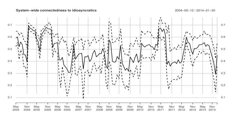
Figure 1: Top panel: System-Wide Connectedness ($C^{H}$); Center panel: System-Wide Connectedness due to Market ($C^{H}_{Mkt}$); Bottom panel: System-Wide Connectedness due to Idiosyncratics ($C^{H}_{Ids}$). Span: 2003-2013, 150 days rolling window.

Starting from $C^{H}$, in Figure 1 we find a similar shape of the SWC as computed in Demirer et al., (2018) (see especially their Figure 9). With the Federal Reserve decision to tighten monetary policy in May-June 2006, we observe an upward trending behavior of the SWC culminating in the Lehamn bankrupcy in September 2008. The level of SWC and its magnitude change is however slightly different from the one computed in Demirer et al., (2018). They find $C^{H}$ to pass from roughly 60% connectedness in 2004, to more than 85% between 2008-2009. In our case, SWC passes from 70% to more than 95% in 2008-2009. This gives a picture of a very interconnected system of global banks, which are even more interconnected, acting cohesively, during global crises. The reason why we find a 10-15% difference in connectedness magnitude with respect to Demirer et al., (2018) is hard to trace exactly, since the approximating model is substantially different and the tuning of the parameters is too. However, it is clear how the VAR Elastic Net of Demirer et al., (2018) directly “sparsifies” the number of banks in every estimate of the VAR equations, while we only shrink part of the connections among different cross-sections. This entails that if truly factors are playing a role, then such direct sparsity is also implicitly shrinking the loadings. In our case, the factor model does not impose direct sparsity on the linkages of $\bm{x}_{t}$, nor on the loadings, but retains one strong factor representing the common behavior of all banks. Instead, we just sparsify the idiosyncratics’ dynamic, which as discussed is a more reasonable consideration. In other words, the assumption of sparsity of Demirer et al., (2018) can potentially lead to underestimation of the degree of connectedness if truly the data linkages are many and if the factors are strong. Furthermore, the fact that SWC is generally ’quite high’ in our results, resonates well with the findings in a.o., Allen & Gale, (2000), Freixas et al., (2000), Acemoglu et al., (2015). Namely, that when the magnitude of the shocks is below a certain threshold, “a more diversified pattern of inter bank liabilities leads to a less fragile financial system”. The other way around, if the shocks’ magnitude surpasses a certain threshold “highly diversified lending patterns facilitate financial contagion and create a more fragile system” (Acemoglu et al.,, 2015, pg. 566). In other words, that the SWC is generally high is not surprising, what we can add here to the discussion is that this threshold between “high” and “too high” can be identified as attained when the share of SWC is proportionally more driven by common, rather than idiosyncratic variation, as we discuss below.

As visible from Figure 1 top panel, the Lehman bankruptcy raised the global connectedness by over 25% compared to the baseline profile in 2003. While 2008 is the highest peak of SWC, it is tightly followed by the one starting at the end of 2010, peaking in 2011 and recovering in spring 2012. This aligns with the period during which Italy and Spain became part of the group of EU nations that were taken aback by the unfolding events in the banking and sovereign debt markets. The level of connectedness surpasses the 95% threshold then, only to rapidly revert back to a 75-80% level in roughly 10 months span. Undeniably, the subprime crisis in 2007-2008 has risen the overall level of SWC, and this has probably remained “sticky” from 2008 all the way to the end of 2010, before starting to revert back to its original pre-crisis level. What is mostly interesting, though, is to observe by what types of shocks (market/idiosyncratics) –and when– the SWC is driven from, i.e., looking at $C^{H}_{Mkt},C^{H}_{Ids}$, respectively second and third panel of Figure 1. Interestingly, we observe how the connectedness is mostly driven by idiosyncratic variation. In normal times, i.e., when no crises are on the horizon, $\approx$60-80% of SWC is due to idiosyncratic variation, while only $\approx$20-40% is due to the market shocks. For example, looking at the span May 2004-May 2006, SWC fluctuates between 70-80% connectedness, so on average 75%, of which 55-60% is due to idiosyncratics ($\approx$80%), and 15-20% is due to the market ($\approx$20%). Similarly, in the periods between December 2009-December 2010 and that between summer 2012 and January 2014, SWC has an average of $\approx$80%, of which $\approx$50% is idiosyncratics and $\approx$30% is market. This seems to be saying that in normal times the stock price volatilities of the banks are interconnected, but what drives the connection is what/how the single banks are doing and their own specific shocks. Therefore, in normal times an idiosyncratic shock such as e.g., the recent case of the collapse of Silicon Valley Bank in 2023, can have a sizeable impact on the SWC. Therefore, stock prices are much less decided by a “market” dynamic when times are calm, but rather by a combination of the banks individual behaviors, so that these idiosyncratic shocks can play a major role in determining global future uncertainty in the banking market.

This phenomenon of idiosyncratic variation driving the connectedness gets quite ’flipped around’ whenever a major crisis occurs: it is clearly visible how the subprime financial crisis has rapidly increased the SWC to Market $C^{H}_{Mkt}$, first with a level shift from 20% between 2003-2006, to 40% between May 2006 and summer 2008, and peaking at more than 60% connectedness in September 2008. In a mirrored way, the SWC to idiosyncratics dropped from 60% to 40%, touching its lowest at almost 30% at the Lehman bankruptcy. Similarly, the financial turmoils within the EU in 2010-2011 have caused again an increase in $C^{H}_{Mkt}$ to almost 60% and a consequent decrease of $C^{H}_{Ids}$ to 40% between 2011 and 2012. Whenever idiosyncratic shocks spread increasing “panic” on the market, the SWC starts to increase and be driven increasingly more by a common dynamic. This seems also to reflect some human psychological dynamic for which in times of uncertainty entities prefers to “gather round” rather than act more independently (cf. “herd behavior”). Of course, here we are talking about stock price volatilities, yet it is sensible to speculate that when uncertainty is high, risk aversion is high(er) too, and banks prefer to act more “compactly” as a market, rather than independently, thing this that is reflected on the connectedness of their stock price volatilities.

Concerning the statistical guarantees of such connectedness measures, we observe that the 95% confidence bands are quite narrow for the SWC, considering the scale. For $C^{H}$ there seems to be a wider upper interval of roughly 2% towards lower/higher connectedness. For $C^{H}_{Mkt}$ and $C^{H}_{Ids}$ the bands appear to be a bit wider, especially in the two main crisis episodes of 2008 and 2010-2011. For $C^{H}_{Mkt}$ the upper end of the interval almost arrives touching a 20% uncertainty towards even higher connectedness in both 2008 and 2010-2011, while it is around 10-15% in normal times. The lower end instead is a bit tighter to the estimated line with roughly 10% distance or less throughout. In a mirrored way for the SWC to idiosyncratics, the lower end of the interval is wider of 10-15% with peaks of 20% in crisis periods, while the upper end is 10% distant or less throughout.

3.2 Dataset (ii): 2014-2023

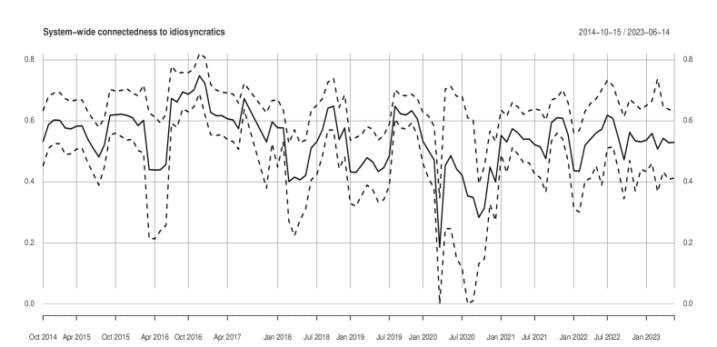
Figure 2: Top panel: System-Wide Connectedness ($C^{H}$); Center panel: System-Wide Connectedness due to Market ($C^{H}_{Mkt}$); Bottom panel: System-Wide Connectedness due to Idiosyncratics ($C^{H}_{Ids}$). Span: 2014-2023, 150 days rolling window.

Now we discuss the connectedness results in Figure 2 on our more recent (2014-2023) dataset, containing almost the same variables (some are discontinued, see Table LABEL:Bank_List for a list) as in the previous analysis. The level of SWC seems to be picking up from where was left after January 2014 in the previous analysis. $C^{H}$ has less of a clearly trending behavior in this new sample period but more of an oscillatory one around 80-85%. The main events of relevance within the sample are of course the Covid19 outbreak and the consequent global crisis starting in 2019, as well as the Ukraine invasion by Russia in February 2022. In both cases, a visible upward jump of the SWC is visible. The Covid19 outbreak lets the SWC jump a steep total of roughly 20% connectedness, from 75-80% to roughly 98%. Less is observed for the Russia-Ukraine war, where a first increase of roughly 5% of SWC can be seen after the Russian invasion in February 2022 and then the SWC oscillates between 85-90% connectedness. SWC to Market, $C^{H}_{Mkt}$ is attested at a consistent 20-35% up to the Covid19 outbreak in 2019 and in the aftermath of the Covid19 crisis between summer 2020 and June 2022. Covid19 has undeniably been a huge global, common shock, affecting in a cross sectional manner all markets. $C^{H}_{Mkt}$ jumps from roughly 15% up to 80% first, then levels off at 60% and at this level it stays for a bit less than a whole year before starting to drop down again to its original pre-crisis level. The war in Ukraine does not seem to have impacted the financial markets as much. $C^{H}_{Mkt}$ does not show particular increases besides Januay 2022 when it touches 40%, but otherwise oscillates around 30%. Once again, when looking at $C^{H}_{Ids}$ we observe the mirrored picture of $C^{H}_{Mkt}$. We see how SWC is driven 70-80% by idiosyncratic variation in normal times, and this level dramatically drops to roughly 20% during the Covid19 crisis.

Concerning the confidence bands, the overall picture seems similar to the previous analysis, with possibly just slightly wider bands around the Covid19 crisis. For $C^{H}$ and $C^{H}_{Mkt}$ the upper confidence band are, respectively, $\approx$2% and $\approx$10% farther from the estimated connectedness. Similarly, for the lower bands. One interesting thing to notice is that the Covid19 outbreak happens around December 2019, at that time SWC is slightly lower than 80%, of which more than 60% is due to idiosyncratic variation. Once understood and experienced the scale of the pandemic, the sum of the single panicking banks on the market made the SWC increase vertically, driven by the rapid increase of $C^{H}_{Mkt}$, accompanied by a mirrored decrease in $C^{H}_{Ids}$. Hence, the scale of the panic (uncertainty) is possibly what decides the speed of increase/decrease of $C^{H}_{Mkt}$/$C^{H}_{Ids}$.

3.3 Comparison of Major Crisis

In the previous two analysis we observed three, very different, types of global crisis within the time spans considered. These are: (i) the 2008 subprime crisis, (ii) the Covid19 pandemic outbreak in 2019, (iii) the war in Ukraine in 2022-2023. As for (i), this is a prototypical financial collapse, while (ii) is a global health crisis and (iii) is an international conflict. Each of these, in their own ways, are responsible for an increased level of global economic uncertainty, and in some cases of proper panic-spreading in the financial markets (aside of elsewhere). We have seen how in all three cases, in line with Demirer et al., (2018), we find global crises correspond to an increase in the overall SWC. However, we have been able to uncover how global crises correspond also to a sharp increase in the connectedness due to the common component (market dynamic), in line with e.g., Barigozzi et al., (2021), and interestingly an almost mirrored sharp decrease in the connectedness due to the idiosyncratics. While all (i)-(iii) crises are in their own way somewhat unprecedented events, the financial crisis in 2008 and the Russia-Ukraine conflict have quite a different shape with respect to the Covid19 pandemic. Crisis (i) is clearly “closer to heart” to the type of data we are looking at here. Banks seem to have perceived this upcoming collapse quite some years in advance, as visible from the building-up pattern of $C^{H}$ from late 2004 onwards, all the way to 2008 (see also Barrell & Davis,, 2008). It also seems that such a crisis has had a more “sticky” effect for the connectedness, which ever since has maintained a slightly higher level of interconnections than before. The Covid19 crisis instead, it is perhaps the single event which created the most vertical increase in SWC and SWC due to the Market, and correspondingly the most vertical drop in $C^{H}_{Ids}$. Such a global health crisis is of course less “close to heart” with respect to the banking market, yet it created such a global panic to rapidly shoot up $C^{H}$. This finding is in line with e.g., Bouri et al., (2021), who also find Covid19 has altered the network of (in their case return) connectedness by generating sudden increases in the system-wide connectedness. The reached peak of $C^{H}$ is then maintained roughly for the whole duration of the uncertainty created by the pandemic and the connectedness then recovers –almost at the same vertical pace– the pre-crisis level. The conflict between Russia and Ukraine is yet another type of crisis, which we cannot observe in its entirety from our available sample at the time of writing. While these types of crises are unfortunately some the world is more accustomed to, the reflections on global energy prices have undoubtedly created global uncertainty which led to increased $C^{H}$, once again. The magnitude of the increase and the clear driving force of $C^{H}_{Mkt}$ are much less clear though. This could be because the financial market, and specifically the banking market has not been particularly directly affected by this event, or because some more recent months of data are still missing at the time of writing.

4 Technical Details

4.1 Details on Estimation Procedure

In estimating the dynamic factor model with sparse VAR idiosyncratic components we closely follow the work of Krampe & Margaritella, (2021). We report here a summary of the main assumptions and, importantly, the estimation algorithm. We refer to the said paper for details.

We work with factors $\{\bm{f}_{t}\}$ and idiosyncratics $\{\bm{\xi}_{t}\}$ being second order, uncorrelated stationary processes, both with bounded $\ell_{2}$ innovation covariances and with the idiosyncratics autocovariance matrix bounded in $\ell_{2}$ norm for increasing $N$. Eight finite moments are assumed on the innovation process $\{(\bm{u}_{t}^{\top},\bm{v}_{t}^{\top})^{\top},t\in\mathbb{Z}\}$ and weak factors are ruled out, so each of the factors provides a non-negligible contribution to the variance of each component of $\{\bm{x}_{t}\}.$ For the idiosyncratics VAR($p_{\xi}$) coefficient matrix, approximate row-wise sparsity is assumed and it is allowed to grow with the sample size.

To give the estimation algorithm it is convenient to stack $\bm{x}_{t},$ $t=1,\dots,T$ row-wise in order to obtain $\bm{X}=\bm{\chi}+\bm{\Xi}$ as a $T\times N$ matrix form of the factors & idiosyncratics decomposition $\bm{x}_{t}=\bm{\chi}_{t}+\bm{\xi}_{t}$. The two step estimation procedure then proceeds as follows:

1. Perform a singular value decomposition of

   $$\bm{X}/\sqrt{NT}=\bm{U}_{NT,r}\bm{D}_{NT,r}\bm{V}_{NT,r}^{\top}+\bm{U}_{NT,N-r}\bm{D}_{NT,N-r}\bm{V}_{NT,N-r}^{\top},$$ (11)

   where $\bm{D}_{NT}$ is a diagonal matrix with the singular values arranged in descending order on its diagonal, $\bm{U}_{NT}$ and $\bm{V}_{NT}$ are the corresponding left and right singular vectors. $\bm{U}_{NT,r}\bm{D}_{NT,r}\bm{V}_{NT,r}^{\top}$ corresponds to the $r$ largest elements in $\bm{D}_{NT}$, $\bm{U}_{NT}$ and $\bm{V}_{NT}$.

   Set $\hat{\bm{F}}=\sqrt{T}\bm{U}_{NT,r}$, $\hat{\bm{\Lambda}}=\sqrt{N}\bm{V}_{NT,r}\bm{D}_{NT,r}$, and $\hat{\bm{\xi}}=\bm{X}-\hat{\bm{F}}\hat{\bm{\Lambda}}^{\top}$.
   The VAR($p_{f}$) for the factors is then given by $\hat{\bm{f}}_{t}=\hat{\bm{\Lambda}}\sum_{j=1}^{p_{f}}\bm{D}^{(j)}\hat{\bm{f}}_{t-j}+\bm{u}_{t}.$

2. Let $\hat{\bm{\xi}}_{t}^{v}=(\hat{\bm{\xi}}_{t}^{\top},\dots,\hat{\bm{\xi}}_{t-p_{\xi}}^{\top})^{\top}$. Then, an adaptive LASSO estimator for $\bm{\beta}^{(j)}$ i.e., the $j$th row of $(\bm{B}^{(1)},\dots,\allowbreak\bm{B}^{(p_{\xi})}),$ is given by

   $$\hat{\bm{\beta}}^{(j)}=\operatorname*{arg\,min}_{\bm{\beta}\in\mathds{R}^{Np_{\xi}}}\frac{1}{T-p_{\xi}}\sum_{t=p_{\xi}+1}^{T}(\hat{\xi}_{j,t}-\bm{\beta}^{\top}\hat{\bm{\xi}}_{t-1}^{v})^{2}+\lambda\sum_{i=1}^{Np_{\xi}}|g_{i}\beta_{i}|,\quad j=1,\dots,N,$$ (12)

   where $\lambda$ is a non-negative tuning parameter which determines the strength of the penalty and $g_{i},i=1,\dots,Np_{\xi},$ are weights. For instance, $g_{i}=1$ leads to the standard LASSO. Let also $(\hat{\bm{B}}^{(1)},\dots,\hat{\bm{B}}^{(p_{\xi})})$ be the matrices that correspond to stacking $\hat{\bm{\beta}}^{(j)},j=1,\dots,N$.

In order to select $r,p_{f}$ in (1.) and $p_{\xi}$ in (2.) the following joint extended information criterion is used, letting $Pen=\big{(}rp_{f}+\sum_{j=1}^{p_{\xi}}\|\bm{e}_{i}^{\top}\hat{\bm{B}}^{(j)}\|_{0}\big{)}\frac{\log(T)}{T}C_{T}$, for $i=1,\ldots,N$, then

$$IC_{T,N}^{(i)}:= \underset{r,p_{\xi},p_{f}}{\operatorname*{arg\,min}}\;\ln\bigg{[}{\frac{1}{T}\!\!\!\!\sum_{t=1+\max(p_{\xi},p_{f})}^{T}\!\!\bigg{(}x_{i,t}-\sum_{j=1}^{p_{f}}\hat{\bm{\Lambda}}_{i}^{\top}\hat{\bm{D}}^{(j)}\hat{\bm{f}}_{t-j}-\sum_{j=1}^{p_{\xi}}\bm{e}_{i}^{\top}\hat{\bm{B}}^{(j)}\hat{\bm{\xi}}_{t}^{(r)}\bigg{)}^{2}}\bigg{]}+Pen,$$ (13)

where $C_{T}=c\frac{\log(NT/(N+T))}{\log(T)}$ with $c=1/2$.

In order to select $\lambda$ in (2.) standard Bayesian information criterion is used.

4.2 Bootstrap Confidence Bands

Let $\hat{\bm{\varSigma}}_{v}^{(re)}$ be a regularized version of the sample covariance matrix $\hat{\bm{\varSigma}}_{v}$, i.e., using regularization such as thresholding (Bickel & Levina,, 2008), CLIME (Cai et al.,, 2011) or graphical LASSO (Meinshausen & Bühlmann,, 2006, Friedman et al.,, 2008). We use here the graphical LASSO which puts sparsity constraints on $\bm{\varSigma}_{v}^{-1}$.

1. Generate pseudo innovations $\{\bm{\eta}_{t}^{*},t\in\mathds{Z}\},$ where $\bm{\eta}_{t}^{*}=((\bm{u}_{t}^{*})^{\top},(\bm{v}_{t}^{*})^{\top})^{\top}$ by drawing $\bm{u}^{*}\overset{i.i.d.}{\sim}\mathcal{N}(0,\hat{\bm{\varSigma}}_{u})$ and $\bm{v}^{*}\overset{i.i.d.}{\sim}\mathcal{N}(0,\hat{\bm{\varSigma}}_{v}^{(re)})$.

2. Generate a pseudo factor series $\{\bm{f}_{t}^{*}\}$ by using the VAR$(p_{f})$ model equation, that is $\bm{f}_{t}^{*}=\sum_{j=1}^{p_{f}}\hat{\bm{D}}^{(j)}{\bm{f}^{*}}_{t-j}+\bm{u}_{t}^{*}$ and a burn-in phase. Generate a pseudo idiosyncratic series $\{\bm{\xi}_{t}^{*}\}$ by using the VAR$(p_{\xi})$ model equation, that is $\bm{\xi}_{t}^{*}=\sum_{j=1}^{p_{\xi}}\hat{\bm{B}}^{(j)}{\bm{\xi}^{*}}_{t-j}+\bm{v}_{t}^{*}$ and a burn-in phase. Use the factor model equation to generate a pseudo time series $\bm{x}_{t}^{*}=\hat{\bm{\Lambda}}_{i}^{\top}\bm{f}_{t}^{*}+\bm{\xi}_{t}^{*},t=1,2,\dots,T$.

3. Using the pseudo time series $\{\bm{x}_{t}^{*}\}$, estimate a factor models, i.e., the loadings, factors, and idiosyncratic part as in (11). This gives $\hat{\bm{f}}_{t}^{*},\hat{\bm{\Lambda}}^{*},\hat{\bm{\xi}}_{t}^{*}$. Additionally, estimate a VAR model on the factors and a sparse VAR model on the idiosyncratics as described in step (1.) and (2.) of the previous algorithm. This leads to $\hat{\bm{D}^{*}}^{(j)},j=1,\dots,p_{f},\hat{\bm{B}^{*}}^{(j)},j=1,\dots,p_{\xi}$.

4. Follow Krampe et al., (2023) and compute the de-sparsified MA-matrices $\hat{\bm{\psi}}_{\xi}^{*,(de),(j)},j=1,\dots,H$ based on $\hat{\bm{\xi}}_{t}^{*}$ and the estimated sparse VAR $\hat{\bm{B}^{*}}^{(j)},j=1,\dots,p_{\xi}$. Additionally, estimate the variance of $\hat{\bm{v}_{t}}^{*}$ leading to $\hat{\bm{\Sigma}}_{v}^{*}$.

5. Using $\hat{\bm{\psi}}_{f}^{*,(j)},\hat{\bm{\psi}}_{\xi}^{*,(de),(j)}\;\text{for}\;j=1,\dots,H,\;\text{and}\;\hat{\bm{\Sigma}}_{u}^{*},\hat{\bm{\Sigma}}_{v}^{*}$, compute the FEVD as in (7) leading to $\hat{\theta}_{ij}^{g}(H)^{*},i=1,\dots,N,j=1,\dots,N+r$.

6. Approximate the distribution of $\sqrt{T}(\hat{\theta}_{ij}^{g}(H)-\theta_{ij}^{g}(H))$ by the distribution of the bootstrap analogue $\sqrt{T}(\hat{\theta}_{ij}^{g}(H)^{*}-\hat{\theta}_{ij}^{g}(H))$ for $i=1,\dots,N,j=1,\dots,N+r$.

5 Conclusion

We disentangle the high-dimensional global bank network connectedness index of Diebold & Yılmaz, (2014), Demirer et al., (2018) into connectedness due to market shocks, and connectedness due to idiosyncratic shocks. To do so, instead of regularizing the high-dimensional vector of banks via sparsity-inducing estimators, we leverage on the recent literature bridging factor models with sparse ones. We indeed estimate a dynamic factor model with sparse VAR idiosyncratic components and we are therefore able to decompose the connectedness into the said two parts, as well as provide bootstrap confidence bands for these measures. We find out that idiosyncratic variation is mostly responsible for the highly interconnected network of banks stock price volatilities in normal times. When major crisis occur though, like 2008 financial crisis, Covid19, and the war in Ukraine, the situation gets completely reversed: bank stock price volatilities tends then to be even more connected and the connections are driven by a market dynamic and not anymore by an idiosyncratic dynamic.

While our proposed framework is employed here to estimate connectedness networks, it can most definitely be employed for high-dimensional impulse response analysis to identify the response to either a shock in the market, an idiosyncratic shock, or even a combination of those. Also, a frequency-domain extension can be quite easily achieved by using again the theory developed in Krampe & Margaritella, (2021). This might be an interesting avenue for future research if one is interested in accounting for different frequencies in the response to either type of shocks.

Appendix A Global Bank Detail, by Assets

Here we provide detail on our sample of all 96 publicly-traded banks in the world’s top 150 (by assets). In Table LABEL:Bank_List we show the banks ordered by assets, and we provide market capitalizations and assets (both in billions of U.S. dollars), our bank codes (which shows country), and Reuters tickers. The last column indicates with a tick if the bank is included in the new dataset from 2014 till 2023, or with a cross if not.

Table A1: Global Bank Detail (Ordered by Assets)

Bank	Country	Mcap	Asset	Bank	Reuters	Dataset (ii)
Name				Code	Ticker
HSBC Holdings	UK	2010	2.671	hsba.gb	hsba.ln	✓
Mitsubishi UFJ Financial Group	Japan	822	2.504	mtbh.jp	X8306.to	✓
BNP Paribas	France	1000	2.482	bnp.fr	bnp.fr	✓
JPMorgan Chase & Co	US	2180	2.416	jpm.us	jpm	✓
Deutsche Bank	Germany	498	2.224	dbk.de	dbk.xe	✓
Barclays	UK	682	2.174	barc.gb	barc.ln	✓
Credit Agricole	France	367	2.119	aca.fr	aca.fr	✓
Bank of America	US	1770	2.102	bac.us	bac	✓
Citigroup	US	1500	1.880	c.us	c	✓
Mizuho Financial Group	Japan	497	1.706	mzh.jp	8411.to	✓
Societe Generale	France	516	1.703	gle.fr	gle.fr	✓
Royal Bank of Scotland Group	UK	356	1.703	rbs.gb	rbs.ln	✗
Sumitomo Mitsui Financial Group	Japan	643	1.567	smtm.jp	8316.to	✓
Banco Santander	Spain	1030	1.538	san.es	san.mc	✓
Wells Fargo	US	2430	1.527	wfc.us	wfc	✓
ING Groep	Netherland	557	1.490	inga.nl	inga.ae	✓
Lloyds Banking Group	UK	961	1.403	lloy.gb	lloy.ln	✓
Unicredit	Italy	477	1.166	ucg.it	ucg.mi	✓
UBS	Switzerland	802	1.138	ubsn.ch	ubsn.vx	✓
Credit Suisse Group	Switzerland	503	983	csgn.ch	csgn.vx	✓
Goldman Sachs Group	US	742	912	gs.us	gs	✓
Nordea Bank	Sweden	556	870	nor.se	ndasek.sk	✓
Intesa Sanpaolo	Italy	458	864	isp.it	isp.mi	✓
Morgan Stanley	US	577	833	ms.us	ms	✓
Toronto-Dominion Bank	Canada	827	827	td.ca	td.t	✓
Royal Bank of Canada	Canada	935	825	ry.ca	ry.t	✓
Banco Bilbao Vizcaya Argentaria	Spain	708	803	bbva.es	bbva.mc	✓
Commerzbank	Germany	206	759	cbk.de	cbk.xe	✓
National Australia Bank	Australia	724	755	nab.au	nab.au	✓
Bank of Nova Scotia	Canada	698	713	bns.ca	bns.t	✓
Commonwealth Bank of Australia	Australia	1100	688	cba.au	cba.au	✓
Standard Chartered	UK	524	674	stan.gb	stan.ln	✓
China Merchants Bank	China	358	664	cmb.cn	600036.sh	✗
Australia and New Zealand Banking Group	Australia	776	656	anz.au	anz.au	✗
Westpac Banking	Australia	918	650	wbc.au	wbc.au	✓
Shanghai Pudong Development Bank	China	295	608	shgp.cn	600000.sh	✗
Danske Bank	Denmark	256	597	dan.dk	danske.ko	✓
Sberbank Rossii	Russia	594	552	sber.ru	sber.mz	✓
China Minsheng Banking Corp	China	297	533	cmb.cn	600016.sh	✓
Bank of Montreal	Canada	419	515	bmo.ca	bmo.t	✓
Itau Unibanco Holding	Brazil	332	435	itub4.br	itub4.br	✓
Resona Holdings	Japan	122	434	rsnh.jp	8308.to	✓
Nomura Holdings	Japan	256	422	nmrh.jp	8604.to	✓
Sumitomo Mitsui Trust Holdings	Japan	184	406	smtm.jp	8309.to	✓
State Bank of India	India	165	400	sbin.in	sbin.in	✓
DNB ASA	Norway	289	396	dnb.no	dnb.os	✓
Svenska Handelsbanken	Sweden	309	388	shba.se	shba.sk	✓
Skandinaviska Enskilda Banken	Sweden	291	387	seba.se	seba.sk	✓
Canadian Bank of Commerce	Canada	324	382	cm.ca	cm.t	✓
Bank of New York Mellon	US	363	374	bk.us	bk.us	✓
U.S. Bancorp	US	745	364	usb.us	usb	✓
Banco Bradesco	Brazil	235	355	bbdc4.br	bbdc4.br	✓
KBC Groupe	Belgium	260	333	kbc.be	kbc.bt	✓
PNC Financial Services Group	US	435	320	pnc.us	pnc.us	✓
DBS Group Holdings	Singapore	320	318	d05.sg	d05.sg	✓
Ping An Bank	China	190	313	pab.cn	000001.sz	✓
Woori Finance Holdings	Korea	84	309	wrfh.kr	053000.se	✗
Dexia	Belgium	1	307	dexb.be	dexb.bt	✗
Capital One Financial	US	415	297	cof.us	cof	✓
Shinhan Financial Group	Korea	188	295	shf.kr	055550.se	✓
Swedbank	Sweden	308	284	swe.se	sweda.sk	✓
Hua Xia Bank	China	124	276	hxb.cn	600015.sh	✓
Erste Group Bank	Austria	168	276	ebs.at	ebs.vi	✓
Banca Monte dei Paschi di Siena	Italy	29	275	bmps.it	bmps.mi	✓
State Street Corporation	US	30	243	stt.us	stt.us	✓
Banco de Sabadell	Spain	131	225	sab.es	sab.mc	✓
United Overseas Bank	Singapore	251	225	uob.sg	u11.sg	✓
Banco Popular Espanol	Spain	13	204	pop.es	pop.mc	✗
Industrial Bank of Korea	Korea	66	193	ibk.kr	024110.se	✓
BB&T Corp	US	266	183	bbt.us	bbt	✗
Bank of Ireland	Ireland	146	182	bir.ie	bir.db	✓
National Bank of Canada	Canada	131	180	na.ca	na.t	✓
SunTrust Banks	US	203	175	sti.us	sti.us	✓
Banco Popolare	Italy	36	174	bp.it	bp.mi	✗
Malayan Banking Berhad	Malaysia	263	171	may.my	maybank.ku	✓
Allied Irish Banks	Ireland	999	162	aib.ie	aib.db	✗
Standard Bank Group	South Africa	177	161	sbk.za	sbk.jo	✓
American Express	US	947	153	axp	axp	✓
National Bank of Greece	Greece	121	153	ete.gr	ete.at	✓
Macquarie Group	Australia	160	143	mqg.au	mqg.au	✓
Fukuoka Financial Group	Japan	33	137	ffg.jp	8354.to	✓
Bank Of Yokohama	Japan	63	134	boy.jp	8332.to	✗
Pohjola Bank	Finland	58	132	poh.fi	poh1s.he	✗
Fifth Third Bancorp	US	185	130	fitb.us	fitb.us	✓
Regions Financial	US	143	117	rf.us	rf.us	✓
Chiba Bank	Japan	52	117	cbb.jp	8331.to	✓
Unipol Gruppo Finanziario	Italy	28	116	uni.it	uni.mi	✓
Banco Comercial Portugues	Portugal	51	113	bcp.pr	bcp.lb	✓
CIMB Group Holdings	Malaysia	163	113	cimb.my	cimb.ku	✓
Bank of Baroda	India	37	113	bob.in	bankbaroda.in	✓
Turkiye Is Bankasi	Turkey	89	112	isctr.tr	isctr.is	✓
Banco Espirito Santo	Portugal	71	111	bes.pr	bes.lb	✗
Hokuhoku Financial Group	Japan	25	108	hkf.jp	8377.to	✓
Shizuoka Bank	Japan	61	104	shzb.jp	8355.to	✓
Mediobanca Banca di Credito Finanziario	Italy	85	95	mb.it	mb.mi	✓
Yamaguchi Financial Group	Japan	23	93	yfg.jp	8418.to	✓

References

- Acemoglu et al., (2012) Acemoglu, D., Carvalho, V. M., Ozdaglar, A., & Tahbaz-Salehi, A. (2012). The network origins of aggregate fluctuations. Econometrica, 80(5), 1977–2016.
- Acemoglu et al., (2015) Acemoglu, D., Ozdaglar, A., & Tahbaz-Salehi, A. (2015). Systemic risk and stability in financial networks. American Economic Review, 105(2), 564–608.
- Alizadeh et al., (2002) Alizadeh, S., Brandt, M. W., & Diebold, F. X. (2002). Range-based estimation of stochastic volatility models. The Journal of Finance, 57(3), 1047–1091.
- Allen & Gale, (2000) Allen, F. & Gale, D. (2000). Financial contagion. Journal of political economy, 108(1), 1–33.
- Ando et al., (2022) Ando, T., Greenwood-Nimmo, M., & Shin, Y. (2022). Quantile connectedness: modeling tail behavior in the topology of financial networks. Management Science, 68(4), 2401–2431.
- Bai & Ng, (2006) Bai, J. & Ng, S. (2006). Evaluating latent and observed factors in macroeconomics and finance. Journal of Econometrics, 131(1-2), 507–537.
- Barigozzi & Brownlees, (2019) Barigozzi, M. & Brownlees, C. (2019). Nets: Network estimation for time series. Journal of Applied Econometrics, 34(3), 347–364.
- Barigozzi et al., (2023) Barigozzi, M., Cho, H., & Owens, D. (2023). Fnets: Factor-adjusted network estimation and forecasting for high-dimensional time series. Journal of Business & Economic Statistics, (just-accepted), 1–27.
- Barigozzi & Hallin, (2017) Barigozzi, M. & Hallin, M. (2017). A network analysis of the volatility of high dimensional financial series. Journal of the Royal Statistical Society. Series C (Applied Statistics), (pp. 581–605).
- Barigozzi et al., (2021) Barigozzi, M., Hallin, M., Soccorsi, S., & von Sachs, R. (2021). Time-varying general dynamic factor models and the measurement of financial connectedness. Journal of Econometrics, 222(1), 324–343.
- Barrell & Davis, (2008) Barrell, R. & Davis, E. P. (2008). The evolution of the financial crisis of 2007—8. National Institute economic review, 206, 5–14.
- Bickel & Levina, (2008) Bickel, P. J. & Levina, E. (2008). Covariance regularization by thresholding. The Annals of Statistics, (pp. 2577–2604).
- Billio et al., (2012) Billio, M., Getmansky, M., Lo, A. W., & Pelizzon, L. (2012). Econometric measures of connectedness and systemic risk in the finance and insurance sectors. Journal of financial economics, 104(3), 535–559.
- Boivin & Ng, (2006) Boivin, J. & Ng, S. (2006). Are more data always better for factor analysis? Journal of Econometrics, 132(1), 169–194.
- Bouri et al., (2021) Bouri, E., Cepni, O., Gabauer, D., & Gupta, R. (2021). Return connectedness across asset classes around the covid-19 outbreak. International review of financial analysis, 73, 101646.
- Cai et al., (2011) Cai, T., Liu, W., & Luo, X. (2011). A constrained l1 minimization approach to sparse precision matrix estimation. Journal of the American Statistical Association, 106(494), 594–607.
- Demirer et al., (2018) Demirer, M., Diebold, F. X., Liu, L., & Yilmaz, K. (2018). Estimating global bank network connectedness. Journal of Applied Econometrics, 33(1), 1–15.
- Diebold et al., (2017) Diebold, F. X., Liu, L., & Yilmaz, K. (2017). Commodity connectedness. Technical report, National Bureau of Economic Research.
- Diebold & Yılmaz, (2014) Diebold, F. X. & Yılmaz, K. (2014). On the network topology of variance decompositions: Measuring the connectedness of financial firms. Journal of econometrics, 182(1), 119–134.
- Fan et al., (2023) Fan, J., Masini, R. P., & Medeiros, M. C. (2023). Bridging factor and sparse models. The Annals of Statistics, 51(4), 1692–1717.
- Freixas et al., (2000) Freixas, X., Parigi, B. M., & Rochet, J.-C. (2000). Systemic risk, interbank relations, and liquidity provision by the central bank. Journal of money, credit and banking, (pp. 611–638).
- Friedman et al., (2008) Friedman, J., Hastie, T., & Tibshirani, R. (2008). Sparse inverse covariance estimation with the graphical lasso. Biostatistics, 9(3), 432–441.
- Gagliardini et al., (2020) Gagliardini, P., Ossola, E., & Scaillet, O. (2020). Estimation of large dimensional conditional factor models in finance. Handbook of econometrics, 7, 219–282.
- Giannone et al., (2021) Giannone, D., Lenza, M., & Primiceri, G. E. (2021). Economic predictions with big data: The illusion of sparsity. Econometrica, 89(5), 2409–2437.
- Hecq et al., (2023) Hecq, A., Margaritella, L., & Smeekes, S. (2023). Granger causality testing in high-dimensional vars: a post-double-selection procedure. Journal of Financial Econometrics, 21(3), 915–958.
- Koop et al., (1996) Koop, G., Pesaran, M. H., & Potter, S. M. (1996). Impulse response analysis in nonlinear multivariate models. Journal of econometrics, 74(1), 119–147.
- Krampe & Margaritella, (2021) Krampe, J. & Margaritella, L. (2021). Factor models with sparse var idiosyncratic components. arXiv e-prints, (pp. arXiv–2112).
- Krampe et al., (2023) Krampe, J., Paparoditis, E., & Trenkler, C. (2023). Structural inference in sparse high-dimensional vector autoregressions. Journal of Econometrics, 234(1), 276–300.
- Liu et al., (2022) Liu, B.-Y., Fan, Y., Ji, Q., & Hussain, N. (2022). High-dimensional covar network connectedness for measuring conditional financial contagion and risk spillovers from oil markets to the g20 stock system. Energy Economics, 105, 105749.
- Meinshausen & Bühlmann, (2006) Meinshausen, N. & Bühlmann, P. (2006). High-dimensional graphs and variable selection with the lasso. The Annals of Statistics, (pp. 1436–1462).
- Pesaran & Shin, (1998) Pesaran, H. H. & Shin, Y. (1998). Generalized impulse response analysis in linear multivariate models. Economics letters, 58(1), 17–29.
- Ross, (1976) Ross, S. (1976). The arbitrage pricing theory. Journal of Economic Theory, 13(3), 341–360.
- Sharpe, (1964) Sharpe, W. F. (1964). Capital asset prices: A theory of market equilibrium under conditions of risk. The journal of finance, 19(3), 425–442.
- Stambaugh, (1988) Stambaugh, R. F. (1988). The information in forward rates: Implications for models of the term structure. Journal of Financial Economics, 21(1), 41–70.
- Yi et al., (2018) Yi, S., Xu, Z., & Wang, G.-J. (2018). Volatility connectedness in the cryptocurrency market: Is bitcoin a dominant cryptocurrency? International Review of Financial Analysis, 60, 98–114.