Loops in AdS: From the Spectral Representation to Position Space III

Abstract

We study loop amplitudes in anti de-Sitter space via the spectral representation. We consider loops of spinning fields and in particular gauge fields, and derive various identities connecting different families of loop diagrams, at different loops, different spins, different masses. We derive an analytic expression for the exact 4-point correlation function of large-$N_{f}$ conformal scalar QED in AdS. Additionally, we derive analytic expressions for bulk 2-point functions and boundary 4-point functions for various ”blob diagrams”. Finally we study 4-point ladder diagrams with spinning fields, by using the spectral representation and 6J symbol.

1 Introduction

The importance of anti de-Sitter space-time in physics arises primarily due its role in the AdS/CFT correspondence. The latter is a duality that relates a gravitational theory in AdS with a (non-gravitational) quantum field theory (QFT) theory on the boundary of AdS. Deep insights into quantum gravity have been obtained by studying observables in the boundary conformal field theory (CFT). Vice versa, insights into strongly coupled QFT have been obtained by perturbativily studying the bulk AdS theory.

The bulk theory in fact does not have to be a gravitational theory, and one can consider a non-gravitational QFT defined on AdS. The boundary theory is then a non-local (i.e without a stress tensor) conformal theory. We define our theory via a lagrangian for the bulk fields. The physical observables are AdS scattering amplitudes, which can be obtained via the computation of Feynman diagrams in AdS. The Feynman diagrams with all legs ending on the boundary of AdS define conformal correlators for the boundary conformal theory. AdS Feynman diagrams (often known as Witten diagrams) are generally harder to compute compared to their flat-space companions. Indeed, analtyical results for loop diagrams in AdS are scarce. Various techniques have been employed to perform computations of Witten diagrams: in position space Liu:1998th ; Liu:1998ty ; Dolan:2000ut ; Freedman:1998tz ; DHoker:1998ecp ; Freedman:1998bj ; DHoker:1998bqu ; DHoker:1999mqo ; Zhou:2018sfz , momentum-space Raju:2010by ; Raju:2011mp ; Albayrak:2019asr ; Albayrak:2018tam ; Albayrak:2020fyp ; Albayrak:2020isk , Mellin-space Penedones:2010ue ; Fitzpatrick:2011ia ; Paulos:2011ie ; Rastelli:2017udc ; Rastelli:2016nze ; Cardona:2017tsw ; Yuan:2017vgp ; Yuan:2018qva , spectral techniques Carmi:2018qzm ; Carmi:2019ocp ; Carmi:2021dsn ; Ankur:2023lum , using conformal or super symmetry Aharony:2016dwx ; Henriksson:2017eej ; Alday:2017xua ; Alday:2017gde ; Mazac:2018mdx ; Carmi:2020ekr ; Caron-Huot:2018kta ; Alday:2017vkk ; Aprile:2017bgs ; Aprile:2017qoy ; Bissi:2020woe ; Bissi:2020wtv . For other works on loop amplitudes in AdS see Fitzpatrick:2010zm ; Fitzpatrick:2011hu ; Ponomarev:2019ofr ; Bertan:2018khc ; Bertan:2018afl ; Beccaria:2019stp ; Fitzpatrick:2011dm ; Giombi:2017hpr ; Costantino:2020vdu ; Antunes:2020pof ; Meltzer:2019nbs ; Nagaraj:2020sji ; Meltzer:2020qbr ; Albayrak:2020bso ; Zhou:2020ptb ; Eberhardt:2020ewh .

In the current work we use the spectral representation to study and compute AdS amplitudes at the loop level. We consider both scalar and spinning field in AdS, and study a family of diagrams which we call ”blob diagrams”, which are particularly suseptible to spectral techniques. We derive a set of vertex/propagator identities that relate various diagrams, and these identities enable to compute certain ”blob diagrams” in terms of lower loop (and often tree-level) diagrams. Other identities enable to relate diagrams across different masses, dimensions, and spins. In previous work Ankur:2023lum we initiated a study of large-$N_{F}$ scalar QED on $AdS$. The spectral representation enables to resum bubble diagrams in the bulk, which gives the exact photon propagator at order $1/N_{f}$. This then enables to compute the 4-point functions. We focus here on the bulk conformal point of scalar QED, in which we obtain the analytical expression for the 4-point correlator in position space.

In section 2 we review the spectral representation of bulk 2-point functions of spinning fields in AdS, and of boundary 4-point functions. In section 3 we derive various vertex/propagator identities. In section 4 we study the position-space 4-point correlator in the large-$N_{f}$ scalar QED on $AdS_{3}$. In section 5 we compute bulk AdS 2-point correlators of spinning fields. In section 6 we compute various 4-point 1-loop bubble diagrams. In section 7 we go beyond ”blob diagrams” and consider 4-point ladder diagrams of spinning fields in the spectral representation. In section 8 we summarize the results and discuss future directions. In appendix A we show details of the computation of ladder diagrams. In appendix B we write blob diagrams in terms of Legendre functions. In appendix C we show additional relations for 4-point blob diagrams.

2 The Spectral representation

In this section we discuss the spectral representations of bulk 2-point functions. We first review the spectral representation for scalar and spin-$J$ bulk fields. In subsection 2.3 we compute the 1-loop bubble 2-point function of a spin-$J$ field. In subsection 2.4 we attach bulk-to-boundary propagators to construct boundary 4-point ”blob diagrams”. Spinning AdS propagators and spectral representations were discussed in Costa:2014kfa .

2.1 Spin-0 spectral representation

Consider a scalar field $\phi(x)$ in $AdS_{d+1}$, Its mass $m$ is related to the boundary scaling dimension $\Delta$ as $m^{2}=\Delta(\Delta-d)$, where we are setting the AdS radius to be 1. The bulk-to-bulk propagator between two bulk points $x_{1}$ and $x_{2}$ is:

$$G_{\Delta}(x_{1},x_{2})=\frac{\Gamma_{\Delta}}{2\pi^{\frac{d}{2}}\Gamma_{\Delta-\frac{d}{2}+1}}\zeta^{-\Delta}{}_{2}F_{1}(\Delta,\Delta-\frac{d-1}{2},2\Delta-d+1,-4\zeta^{-1})$$ (1)

Here $\zeta=\frac{(z_{1}-z_{2})^{2}+(\vec{x}_{1}-\vec{x}_{2})^{2}}{z_{1}z_{2}}$ is the chordal distance squared. This propagator has a spectral representation in $\nu$-space as follows:

$$G_{\Delta}(x_{1},x_{2})=\int_{-\infty}^{\infty}\frac{d\nu}{\nu^{2}+(\Delta-\frac{d}{2})^{2}}\Omega_{\nu}(x_{1},x_{2})\ \ \ \ \ ,\ \ \ \ \ \tilde{F}_{\nu}=\frac{1}{\nu^{2}+(\Delta-\frac{d}{2})^{2}}$$ (2)

where $\Omega_{\nu}(x_{1},x_{2})$ is the harmonic function in $AdS_{d+1}$

$$\Omega_{\nu}(x_{1},x_{2})=\frac{i\nu}{2\pi}\Big{(}G_{\frac{d}{2}+i\nu}(x_{1},x_{2})-G_{\frac{d}{2}-i\nu}(x_{1},x_{2})\Big{)}$$ (3)

A general bulk 2-point function $F(x_{1},x_{2})$ in AdS will depend just on the squared chordal distance $\zeta$, see Fig. 1-left. The spectral representation of $F(x_{1},x_{2})$ is:

$$g^{(2)}(\zeta)=F(x_{1},x_{2})=\int_{-\infty}^{\infty}d\nu\tilde{F}_{\nu}\Omega_{\nu}(x_{1},x_{2})\,,$$ (4)

$\tilde{F}_{\nu}$ is a function of $\nu$, and is the spectral transform of $F(x_{1},x_{2})$.

One can obtain CFT boundary correlators by attaching bulk-to-boundary propagators $K_{\Delta_{1}}$ to the 2-point blob $F(x_{1},x_{2})$. For example a 4-point function (see Fig. 1-right):

$$\langle\mathcal{O}_{1}\ldots\mathcal{O}_{4}\rangle=\int d^{d+1}x_{1}d^{d+1}x_{2}F(x_{1},x_{2})K_{\Delta_{1}}(P_{1},x_{1})K_{\Delta_{2}}(P_{2},x_{1})K_{\Delta_{3}}(P_{3},x_{2})K_{\Delta_{4}}(P_{4},x_{2})$$

Here the $P_{i}$ are boundary points. We denote the family of AdS Diagrams in Fig. 1 as ”Blob diagrams”.

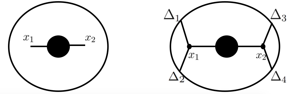
Figure 1: Scalar ”Blob”diagrams. Left: The black blob represents $F(x_{1},x_{2})$, a general bulk scalar two-point function. Other than that, the blob is a completely general function of the geodesic distance. Right: We attach 4 external scalar legs to the boundary, this gives a CFT 4-point function. This is a class of diagrams which has two bulk-to-boundary propagators attached to $x_{2}$, and two attached to $x_{1}$.

2.2 Spin-$J$ spectral representation

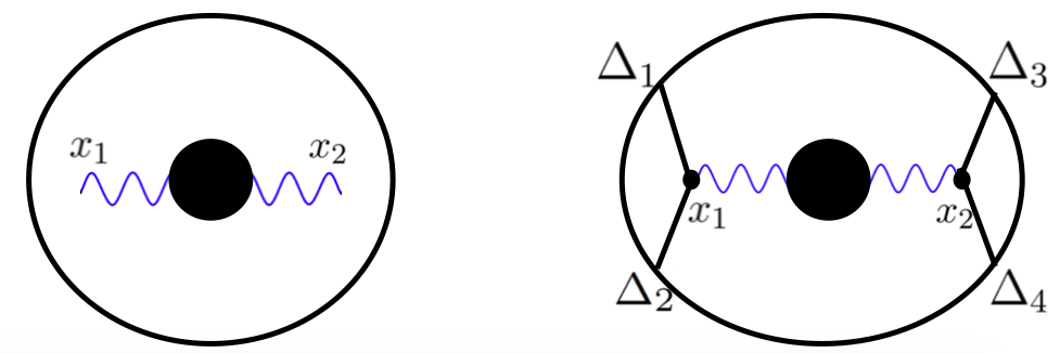
Figure 2: Spinning ”Blob”diagrams. Left: The black blob with wavy lines represents a general bulk spin-$J$ two-point function. Other than that, the blob is completely general. Right: We attach 4 external scalar legs to the boundary, this gives a CFT 4-point function. This is a class of diagrams which has two bulk-to-boundary propagators attached to $x_{2}$, and two attached to $x_{1}$.

We denote the bulk-to-bulk propagator of a spin-$J$ field in AdS by $G_{\Delta,J}(x_{1},x_{2},W_{1},W_{2})$, where $W_{1,2}$ are polarisation vectors. The bulk propagator has a spectral representation Costa:2014kfa :

$$G_{\Delta,J}(x_{1},x_{2},W_{1},W_{2})=\sum_{l=0}^{J}((W_{1}\cdot\nabla_{1})(W_{2}\cdot\nabla_{2}))^{J-l}\int_{-\infty}^{\infty}d\nu a_{l}(\nu)\Omega_{\nu,l}(x_{1},x_{2}:W_{1},W_{2})$$

where $\Omega_{\nu,l}$ is the AdS harmonic function for spin-$l$, and $a_{l}(\nu)$ are $\nu$ dependent functions. For $l=J$, we have $a_{J}(\nu)=\frac{1}{\nu^{2}+(\Delta-\frac{d}{2})^{2}}$.

For a general bulk 2-point function $F_{J}(x_{1},x_{2},W_{1},W_{2})$ of spin-$J$, we have the following spectral representation:

$$F_{J}(x_{1},x_{2},W_{1},W_{2})=\sum_{l=0}^{J}((W_{1}\cdot\nabla_{1})(W_{2}\cdot\nabla_{2}))^{J-l}\int_{-\infty}^{\infty}d\nu F_{\nu,l}\Omega_{\nu,l}(x_{1},x_{2}:W_{1},W_{2})$$

Where the harmonic function in AdS is:

$$\Omega_{\nu,l}(x_{1},x_{2},W_{1},W_{2})=\frac{i\nu}{2\pi}\Big{(}G_{\frac{d}{2}+i\nu,l}(x_{1},x_{2},W_{1},W_{2})-G_{\frac{d}{2}-i\nu,l}(x_{1},x_{2},W_{1},W_{2})\Big{)}$$

The harmonic function has a split representation Costa:2014kfa :

$$\Omega_{\nu,l}(x_{1},x_{2},W_{1},W_{2})=\frac{\nu^{2}}{\pi l!(\frac{d}{2}-1)_{l}}\int d^{d}PK_{\frac{d}{2}+i\nu,l}(x_{1},P,W_{1},D_{Z})K_{\frac{d}{2}-i\nu,l}(x_{2},P,W_{2},Z)$$

where $K_{\frac{d}{2}+i\nu,l}$ is the bulk-to-boundary propagator, and the integration is over the boundary.

2.3 The1-loop bubble spectral representation

Let us recall the results for the 1-loop bubble in the spectral representation. We focus on the case of $AdS_{3}$. The scalar 1-loop bubble spectral representation is Carmi:2018qzm :

$$B(x,y)=\int_{-\infty}^{\infty}d\nu\tilde{B}(\nu)\Omega_{\nu}(x,y)$$ (10)

where

$$\tilde{B}(\nu)=\frac{i}{8\pi\nu}\Big{[}\psi(\Delta-\frac{1+i\nu}{2})-\psi(\Delta-\frac{1-i\nu}{2})\Big{]}$$ (11)

where $\psi$ is the digamma function $\psi(z)\equiv\frac{d}{dz}\log[\Gamma(z)]$, and $\Delta$ is the scaling dimension of the scalar field. This expression simplifies when $\Delta=1$:

$$B(\nu)\Big{|}_{\Delta=1}=-\frac{1}{8i\nu}\cot(\frac{\pi}{2}(1+i\nu))=\frac{1}{16}\frac{\Gamma_{\frac{1}{2}+\frac{i\nu}{2}}\Gamma_{\frac{1}{2}-\frac{i\nu}{2}}}{\Gamma_{1-\frac{i\nu}{2}}\Gamma_{1+\frac{i\nu}{2}}}$$ (12)

In Ankur:2023lum we studied large-$N_{f}$ scalar quantum electrodynamics on $AdS_{d+1}$. The two-point function of the $U(1)$ conserved currents:

$$\langle j_{M}(x)j_{N}(y)\rangle=-\int_{-\infty}^{\infty}d\nu B^{(1)}(\nu)\Omega^{(1)}_{\nu MN}(x,y)$$ (13)

where $B^{(1)}(\nu)$ is the 1-loop bubble in the spectral representation, and $\Omega^{(1)}_{\nu MN}(x,y)$ is the spin-1 AdS harmonic function. For a massless gauge field in $AdS_{3}$, we have

$$B^{(1)}(\nu)=\frac{\nu}{16\pi(\nu^{2}+1)}\Big{(}-2(2\Delta-3)\nu+(\nu^{2}+4(\Delta-1)^{2})(i\psi(\Delta-\frac{i\nu}{2})-i\psi(\Delta+\frac{i\nu}{2}))\Big{)}$$

where $\Delta$ is the scaling dimension of the scalars. This expression simplifies when $\Delta=1$:

$$B^{(1)}(\nu)\Big{|}_{\Delta=1}=\frac{\nu^{3}}{16(\nu^{2}+1)}\coth(\frac{\pi\nu}{2})=-\frac{i\nu^{3}}{16(\nu^{2}+1)}\frac{\Gamma_{1+\frac{i\nu}{2}}\Gamma_{-\frac{i\nu}{2}}}{\Gamma_{\frac{1}{2}-\frac{i\nu}{2}}\Gamma_{\frac{1}{2}+\frac{i\nu}{2}}}$$ (15)

2.4 Boundary correlators: Blob diagrams

One constructs boundary correlators by attaching bulk-to-boundary propagators to the bulk 2-point blob, Fig. 2. For instance the 4-point correlators blob diagrams Costa:2014kfa :

$$\langle\mathcal{O}_{1}\ldots\mathcal{O}_{4}\rangle=\int d^{d+1}x_{1}d^{d+1}x_{2}F_{J}(x_{1},x_{2})\times$$

$$K_{\Delta_{1}}(P_{1},x_{1})[(K_{1}\cdot\nabla_{1})^{J}K_{\Delta_{2}}(P_{2},x_{1})]K_{\Delta_{3}}(P_{3},x_{2}){}[(K_{2}\cdot\nabla_{2})^{J}K_{\Delta_{4}}(P_{4},x_{2})]$$ (16)

Using the spectral representation, the 4-point function becomes:

$$\langle\mathcal{O}_{1}\ldots\mathcal{O}_{4}\rangle=A\sum_{l=0}^{J}\int_{-\infty}^{\infty}d\nu F_{\nu,l}\mathcal{P}^{\Delta_{i}}_{\frac{d}{2}+i\nu,l}(z,\bar{z})$$ (17)

where the cross-ratios are $u=z\bar{z}=\frac{P_{12}P_{34}}{P_{13}P_{24}}$ and $v=(1-z)(1-\bar{z})=\frac{P_{14}P_{23}}{P_{13}P_{24}}$, and we defined:

$$A\equiv 2g_{\phi_{1}\phi_{2}h}g_{\phi_{3}\phi_{4}h}\frac{\Big{(}\frac{P_{24}}{P_{14}}\Big{)}^{a}\Big{(}\frac{P_{14}}{P_{13}}\Big{)}^{b}}{(P_{12})^{a_{p}}(P_{34})^{b_{p}}}$$ (18)

where we defined $a\equiv\frac{\Delta_{1}-\Delta_{2}}{2}$, $b\equiv\frac{\Delta_{3}-\Delta_{4}}{2}$ and $a_{p}\equiv\frac{\Delta_{1}+\Delta_{2}}{2}$, $b_{p}\equiv\frac{\Delta_{3}+\Delta_{4}}{2}$. In Eq. 17, $\mathcal{P}^{\Delta_{i}}_{\frac{d}{2}+i\nu,l}(z,\bar{z})$ is the conformal partial wave.

$$\mathcal{P}^{\Delta_{i}}_{\frac{d}{2}+i\nu,l}(z,\bar{z})=\int dP\langle\mathcal{O}_{\Delta_{1}}(P_{1})\mathcal{O}_{\Delta_{2}}(P_{2})\mathcal{O}_{\frac{d}{2}+i\nu,l}(P,D_{z})\rangle\langle\mathcal{O}_{\frac{d}{2}-i\nu,l}(P,Z)\mathcal{O}_{\Delta_{3}}(P_{3})\mathcal{O}_{\Delta_{4}}(P_{4})\rangle$$ (19)

We can write Eq. 17 as follows:

$$\langle\mathcal{O}_{1}\ldots\mathcal{O}_{4}\rangle=Ag^{(4)}(z,\bar{z})=A\pi^{2}\sum_{l=0}^{J}g_{l}(z,\bar{z})$$ (20)

where

$$\boxed{g_{l}(z,\bar{z})=\int_{-\infty}^{\infty}d\nu\frac{\tilde{F}_{\nu,l}}{\sin\pi(a_{p}-\frac{\frac{d}{2}+i\nu-l}{2})\sin\pi(b_{p}-\frac{\frac{d}{2}+i\nu-l}{2})}\Upsilon_{\nu,l}^{\Delta_{i}}\times\mathcal{K}^{\Delta_{i}}_{\frac{d}{2}+i\nu,l}(z,\bar{z})}$$ (22)

Eq. 20 and 22 give the expansion of the 4-point correlator in terms of conformal blocks $\mathcal{K}^{\Delta_{i}}_{\frac{d}{2}+i\nu,l}(z,\bar{z})$. The poles from the denominator $\sin\pi(a_{p}-\frac{\frac{d}{2}+i\nu-l}{2})\sin\pi(b_{p}-\frac{\frac{d}{2}+i\nu-l}{2})$ give the contribution of the double-trace operators to the conformal block expansion.

We can take the double discontinuity of this expression, which cancels the $sin$ denominators in Eq. 22:

$$dDisc[g_{l}(z,\bar{z})]=\int_{-\infty}^{\infty}d\nu\tilde{F}_{\nu,l}\Upsilon_{\nu,l}^{\Delta_{i}}\times\mathcal{K}^{\Delta_{i}}_{\frac{d}{2}+i\nu,l}(z,\bar{z})$$ (23)

or the single discontinuity:

$$Disc_{a_{p}}[g_{l}(z,\bar{z})]=\int_{-\infty}^{\infty}d\nu\frac{\tilde{F}_{\nu,l}}{\sin\pi(b_{p}-\frac{\frac{d}{2}+i\nu-l}{2})}\Upsilon_{\nu,l}^{\Delta_{i}}\times\mathcal{K}^{\Delta_{i}}_{\frac{d}{2}+i\nu,l}(z,\bar{z})$$ (24)

For example, for contact diagrams we have $\tilde{F}_{\nu,l}=1$, and the previous expression is given from the residue theorem:

$$Disc_{a_{p}}[g_{l}(z,\bar{z})]=\sum_{n=0}^{\infty}\Upsilon_{\nu,l}^{\Delta_{i}}\times\mathcal{K}^{\Delta_{i}}_{\frac{d}{2}+i\nu,l}(z,\bar{z})\Big{|}_{\frac{d}{2}+i\nu\to b_{p}+l+n}$$ (25)

On the other hand, the double-discontinuity gets rid of the double trace poles completely

$$dDisc[g_{l}(z,\bar{z})]=\sum_{n=0}^{\infty}Res[\tilde{F}_{\nu,l}]\Upsilon_{\nu,l}^{\Delta_{i}}\times\mathcal{K}^{\Delta_{i}}_{\frac{d}{2}+i\nu,l}(z,\bar{z})\Big{|}_{\nu=\nu_{n}}$$ (26)

where $\nu_{n}$ are the poles of $F_{\nu,l}$ and $Res[\tilde{F}_{\nu,l}]$ are their residues.

Let us make a few more convenient definitions regarding the gamma functions appearing in Eq. 21:

$$U_{A.V}^{(a_{p},l)}\equiv\Gamma_{a_{p}+\frac{l}{2}+\frac{i\nu-\frac{d}{2}}{2}}\Gamma_{a_{p}+\frac{l}{2}-\frac{i\nu+\frac{d}{2}}{2}}$$ (27)

and

$$U_{V}^{(a_{p},l,\Delta)}\equiv\Gamma_{a_{p}+\frac{l}{2}+\frac{i\nu-\frac{d}{2}}{2}}\Gamma_{a_{p}+\frac{l}{2}-\frac{i\nu+\frac{d}{2}}{2}}\times\frac{1}{\nu^{2}+(\Delta-\frac{d}{2})}$$ (28)

3 Identities for Witten diagrams

In this section we derive various vertex/propagator identities, which will enable to relate different Witten diagrams together.

3.1 Identity 0

For a $CFT_{d}$ with $d=$even, the 4-point conformal blocks contain the following hypergeometric function:

$$k_{\beta}^{(a,b)}(z)\equiv z^{\frac{\beta}{2}}{}_{2}F_{1}(\frac{\beta}{2}+a,\frac{\beta}{2}+b,\beta,z)$$ (29)

Recall that the conformal blocks in $d=2$ and $d=4$ are:

$$\mathcal{K}^{(d=2)}_{\Delta,l}(z,\bar{z})=\frac{1}{1+\delta_{l,0}}\Big{(}k_{\Delta-l}^{(a,b)}(z)k_{\Delta+l}^{(a,b)}(\bar{z})+k_{\Delta+l}^{(a,b)}(z)k_{\Delta-l}^{(a,b)}(\bar{z})\Big{)}$$

$$\mathcal{K}^{(d=4)}_{\Delta,l}(z,\bar{z})=\frac{z\bar{z}}{z-\bar{z}}\Big{(}k_{\Delta-l-2}^{(a,b)}(z)k_{\Delta+l}^{(a,b)}(\bar{z})-k_{\Delta+l}^{(a,b)}(z)k_{\Delta-l-2}^{(a,b)}(\bar{z})\Big{)}$$ (30)

Following Dolan:2011dv , lets define the following differential operators:

$$D^{z}_{+}\equiv z^{1-b}\partial_{z}z^{b}$$

$$D^{z}_{-}f(z)\equiv z^{1+b}(1-z)^{1-a-b}\partial_{z}\Big{[}z^{-b}(1-z)^{a+b}f(z)\Big{]}$$ (31)

Acting with them, raises or lowers $b$ by one Dolan:2011dv :

$$D^{z}_{+}k_{\beta}^{(a,b)}(z)=(\frac{\beta}{2}+b)k_{\beta}^{(a,b+1)}(z)$$

$$D^{z}_{-}k_{\beta}^{(a,b)}(z)=(\frac{\beta}{2}-b)k_{\beta}^{(a,b-1)}(z)$$ (32)

Since the functions $k_{\beta}^{(a,b)}(z)$ are symmetric with respect to to $a$ and $b$, one can likewise define raising/lowering operators for $a$.

3.1.1 $d=2$

In $d=2$, the spectral representation of the 4-point function, Eq. 21 and 22, contains the following factor $\Gamma_{\frac{i\nu+l+1}{2}+b}\Gamma_{\frac{i\nu+l+1}{2}-b}k_{\frac{i\nu+l+1}{2}}^{(a,b)}(z)k_{\frac{i\nu-l+1}{2}}^{(a,b)}(\bar{z})$. Acting with two raising operators gives:

$$D^{\bar{z}}_{+}D^{z}_{+}\Big{[}\Gamma_{\frac{i\nu+l+1}{2}+b}\Gamma_{\frac{i\nu+l+1}{2}-b}k_{i\nu+l+1}^{(a,b)}(z)k_{i\nu-l+1}^{(a,b)}(\bar{z})\Big{]}$$

$$=\frac{-1}{4}(\nu^{2}+(-l+2b+1)^{2})\Big{(}\Gamma_{\frac{i\nu+l+1}{2}+b+1}\Gamma_{\frac{i\nu+l+1}{2}-b-1}k_{i\nu+1+l}^{(a,b+1)}(z)k_{i\nu-l+1}^{(a,b+1)}(\bar{z})\Big{)}$$ (33)

This factor $(\nu^{2}+(-l+2b+1)^{2})$ is the inverse propagator with $\delta=2b+2-l$. Therefore:

$$\textbf{Identity\ 0a:}\ \ \ \ \ \ \ \ \boxed{D^{\bar{z}}_{+}D^{z}_{+}g^{(a,b)}_{l}(z,\bar{z})=\frac{-1}{4}(\nu^{2}+(-l+2b+1)^{2})g^{(a,b+1)}_{l}(z,\bar{z})}$$ (34)

This is shown in Fig. 3.

3.1.2 $d=4$

For $d=4$:

$$D^{\bar{z}}_{+}D^{z}_{+}\Big{[}\Gamma_{\frac{i\nu+l+2}{2}+b}\Gamma_{\frac{i\nu+l+2}{2}-b}k_{i\nu+l+2}^{(a,b)}(z)k_{i\nu-l}^{(a,b)}(\bar{z})\Big{]}$$

$$=\frac{-1}{4}(\nu^{2}+(-l+2b)^{2})\Big{[}\Gamma_{\frac{i\nu+l+2}{2}+b+1}\Gamma_{\frac{i\nu+l+2}{2}-b-1}k_{i\nu+l+2}^{(a,b+1)}(z)k_{i\nu-l}^{(a,b+1)}(\bar{z})\Big{]}$$ (35)

Therefore

$$\textbf{Identity\ 0b:}\ \ \ \ \ \ \ \ \boxed{D^{\bar{z}}_{+}D^{z}_{+}g^{(a,b)}_{l}(z,\bar{z})=\frac{-1}{4}(\nu^{2}+(2b-l)^{2})g^{(a,b+1)}_{l}(z,\bar{z})}$$ (36)

The factor is is the inverse propagator with $\delta=2b-l+2$. This is shown in Fig. 3.

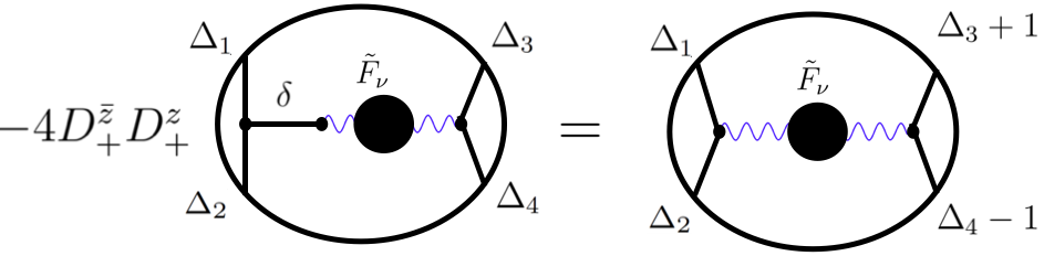
Figure 3: Showing identity 0 in Eqs. 34 and 36. In the LHS we have a scalar propagator with scaling dimension $\delta=2b-l+2$.

3.2 Identity 1

Looking at Eq. 22, $g_{l}^{(\Delta_{i}^{\prime})}(z,\bar{z})$ obeys the following identity:

$$\textbf{Identity\ 1:}\ \ \ \ \ \ \ \ \ \ \ \ \boxed{g_{l}^{(\Delta_{i}^{\prime})}(z,\bar{z})=g_{l}^{(\Delta_{i})}(z,\bar{z})}$$ (37)

where $\Delta_{i}=(\Delta_{1},\Delta_{2},\Delta_{3},\Delta_{4})$ and $\Delta_{i}^{\prime}$ is

$$\Delta_{1}^{\prime}=\Delta_{134,2}\ \ \ ,\ \ \ \Delta_{2}^{\prime}=\Delta_{234,1}\ \ \ ,\ \ \ \Delta_{3}^{\prime}=\Delta_{123,4}\ \ \ ,\ \ \ \Delta_{4}^{\prime}=\Delta_{124,3}$$ (38)

and we defined $\Delta_{123,4}\equiv\frac{\Delta_{1}+\Delta_{2}+\Delta_{3}-\Delta_{4}}{2}$. This identity works exactly the same as for scalar vertex, so it is a simple generalization of identity 1 in section 3.1 of Carmi:2019ocp .

3.3 Identity 2

The conformal block obeys the following eigenvalue equation:

$$2D_{z,\bar{z}}\mathcal{K}_{\frac{d}{2}+i\nu,l}=-\Big{[}\nu^{2}+\frac{d^{2}}{4}-l(d+l-2)\Big{]}\mathcal{K}_{\frac{d}{2}+i\nu,l}$$ (39)

where the differential operator is defined as:

$$D_{z,\bar{z}}\equiv[z^{2}(1-z)\partial_{z}^{2}-(a+b+1)z^{2}\partial_{z}-abz+z\leftrightarrow\bar{z}]$$

$$+(d-2)\frac{z\bar{z}}{z-\bar{z}}[(1-z)\partial_{z}-(1-\bar{z})\partial_{\bar{z}}]$$ (40)

We define (see Eq. 27):

$$U_{A.V}^{(a_{p},l)}\equiv\Gamma_{a_{p}+\frac{l}{2}+\frac{i\nu-\frac{d}{2}}{2}}\Gamma_{a_{p}+\frac{l}{2}-\frac{i\nu+\frac{d}{2}}{2}}$$ (41)

thus

$$U_{A.V}^{(a_{p}-1,l)}\times\Big{(}\frac{-1}{4}\Big{)}\Big{[}2D_{z,\bar{z}}-\alpha)\Big{]}\mathcal{K}_{\frac{d}{2}+i\nu,l}=U_{A.V}^{(a_{p},l)}\mathcal{K}_{\frac{d}{2}+i\nu,l}$$ (42)

where

$$\alpha\equiv 4a_{p}^{2}-2a_{p}(d+4-2l)+2(d+1+l(l-3)$$ (43)

In other words

$$U_{A.V}^{(a_{p}-1,l)}\mathcal{D}^{(+)}_{z,\bar{z}}\mathcal{K}_{\frac{d}{2}+i\nu,l}=U_{A.V}^{(a_{p},l)}\mathcal{K}_{\frac{d}{2}+i\nu,l}$$ (44)

where we defined the differential operator:

$$\mathcal{D}^{(+)}_{z,\bar{z}}\equiv\Big{(}-\frac{1}{4}\Big{)}\Big{[}2D_{z,\bar{z}}-\alpha\Big{]}$$ (45)

We can write this more neatly in terms of the 4-point function $g_{l}$, which gives

$$\textbf{Identity\ 2:}\ \ \ \ \ \ \boxed{g_{l}^{(\Delta_{1},\Delta_{2},\Delta_{3},\Delta_{4})}(z,\bar{z})=\mathcal{D}_{z,\bar{z}}^{(+)}\ \ g_{l}^{(\Delta_{1}-1,\Delta_{2}-1,\Delta_{3},\Delta_{4})}(z,\bar{z})}$$ (46)

This identity is a generalization of identity 2 of Carmi:2019ocp to spinning operators.

3.4 Identity 3

We define (see Eq. 21):

$$U_{V}^{(a_{p},l,\Delta)}\equiv\Gamma_{a_{p}+\frac{l}{2}+\frac{i\nu-\frac{d}{2}}{2}}\Gamma_{a_{p}+\frac{l}{2}-\frac{i\nu+\frac{d}{2}}{2}}\times\frac{1}{\nu^{2}+(\Delta-\frac{d}{2})}$$ (47)

Plugging $\Delta=2a_{p}+l-2$ and recalling Eq. 41, gives:

$$\textbf{Identity\ 3:}\ \ \ \ \ \ \ \ \boxed{U_{V}^{(a_{p},\Delta=2a_{p}+l-2)}=\frac{1}{4}U_{A.V}^{(a_{p}-1)}}$$ (48)

This identity is a generalization of identity 3 of Carmi:2019ocp to spinning operators.

3.5 Identity 4

Let’s look at the sunset diagram in AdS, which in position space is just a product of three propagators. In $d=2$ dimensions, the sunset diagram gives with propagators of scaling dimension $\delta$ is (see Fitzpatrick:2010zm ; Fitzpatrick:2011hu :):

$$G_{\delta}^{3}(x_{1},x_{2})=\sum_{n=0}^{\infty}(n+1)G_{3\delta+2n}(x_{1},x_{2})$$ (49)

Now if we plug $\delta=\Delta+\frac{2}{3}$:

$$G_{\Delta+\frac{2}{3}}^{3}(x_{1},x_{2})=\sum_{n=0}^{\infty}nG_{3\Delta+2n}(x_{1},x_{2})$$ (50)

Subtracting the previous two equations gives:

$$G_{\Delta}^{3}(x_{1},x_{2})-G_{\Delta+\frac{2}{3}}^{3}(x_{1},x_{2})=\sum_{n=0}^{\infty}G_{3\Delta+2n}(x_{1},x_{2})=G_{\frac{3}{2}\Delta}^{2}(x_{1},x_{2})=B(\delta=\frac{3}{2}\Delta)$$ (51)

The RHS is just a bubble diagrams. Therefore in the spectral representation the above equation becomes:

$$\textbf{Identity\ 4a:}\ \ \ \ \ \ \ \ \ \ \ \ \boxed{B^{\Delta}_{sun}(\nu)-B^{\Delta+\frac{2}{3}}_{sun}(\nu)=B^{\frac{3\Delta}{2}}(\nu)}$$ (52)

This identity is shown in Fig. 4

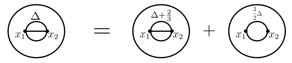
Figure 4: Showing identity 4a of Eq. 52: Relating 2-loop sunset diagrams with different scaling dimensions to the 1-loop bubble diagram.

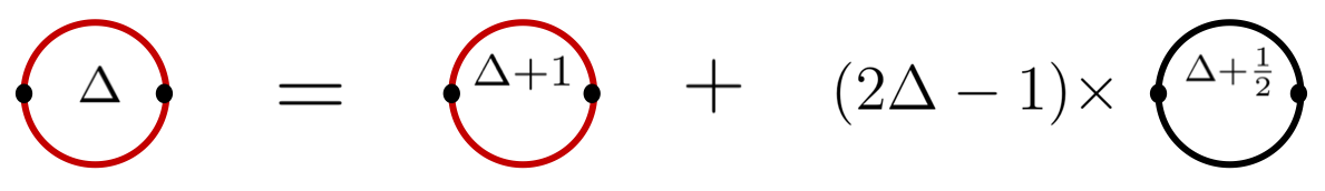
Figure 5: Showing identity 4b of Eq. 56: Relating 1-loop fermionic bubbles. The red lines denote fermionic bulk propagators, whereas the black line denote scalar propagators. This identity can be used inside of Witten diagrams.

Now let us derive an identity for the fermionic bubble. The fermionic bubble in $d=2$ with scaling dimension $\Delta$ is (see section 6 of Carmi:2018qzm ):

$$(G^{F}_{\Delta})^{2}=\sum_{n=0}^{\infty}(n+1)(2\Delta+n-1)G_{2\Delta+2n+1}$$ (53)

Therefore with scaling dimension $\Delta\to\Delta+1$, we have:

$$(G^{F}_{\Delta+1})^{2}=\sum_{n=0}^{\infty}n(2\Delta+n)G_{2\Delta+2n+1}$$ (54)

Subtracting the previous two equations gives the scalar bubble function $G^{B}$ :

$$(G^{F}_{\Delta})^{2}-(G^{F}_{\Delta+1})^{2}=(2\Delta-1)\sum_{n=0}^{\infty}G_{2\Delta+2n+1}=(2\Delta-1)(G^{B}_{\Delta+\frac{1}{2}})^{2}$$ (55)

This gives identity 4b, for the 1-loop bubble of fermions:

$$\textbf{Identity\ 4b:}\ \ \ \ \ \ \ \ \ \ \ \ \boxed{(G^{F}_{\Delta})^{2}=(G^{F}_{\Delta+1})^{2}+(2\Delta-1)(G^{B}_{\Delta+\frac{1}{2}})^{2}}$$ (56)

where $G^{B}_{\Delta+\frac{1}{2}}$ is the scalar bubble. This identity is shown in Fig. 5.

3.6 Identity 6

Let us define

$$U_{B}^{(a_{p},\Delta,l)}\equiv\frac{1}{\nu^{2}}\Gamma_{a_{p}+\frac{l}{2}-\frac{d}{4}-\frac{i\nu}{2}}\Gamma_{a_{p}+\frac{l}{2}-\frac{d}{4}+\frac{i\nu}{2}}B^{(\Delta,l)}_{\nu}$$ (57)

where $B^{(\Delta,l)}_{\nu}$ is the spectral representation of the 1-loop bubble, see section 2.3. Let’s focus on the case of $AdS_{3}$ and $l=1$ and $\Delta=1$ in the bubble., In this case the bubble spectral representation simplifies to a product of gamma functions, as in Eq. 15. From Eqs. 57, 15. and 27, we get

$$\textbf{Identity\ 6:}\ \ \ \ \ \ \boxed{U_{B}^{(a_{p}=\frac{3}{2},\Delta=1,l=1)}=\frac{1}{32}U_{A.V}^{(a_{p}=1,l=1)}}$$ (58)

This identity will help relate loop diagrams to lower loop diagrams or tree level diagrams. We show several examples of this in Fig. 6.

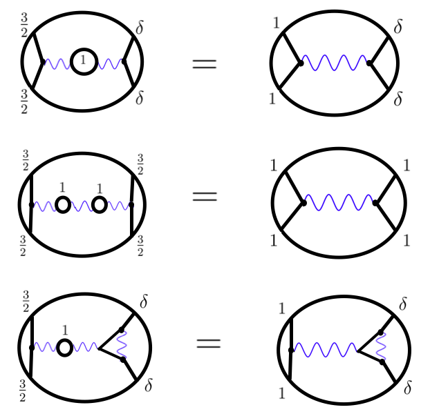
Figure 6: Using identity 6 to reduce loop diagrams to lower loop diagrams in several examples. $\delta$ is a general scaling dimension. Top: A 1-loop bubble diagram that reduces to the tree-level exchange diagram on the right. Middle: A 2-loop bubble diagram that reduces to the tree-level exchange diagram. Bottom: A 2-loop diagram that reduces to a 1-loop diagram.

4 Large-$N_{f}$ scalar QED on AdS

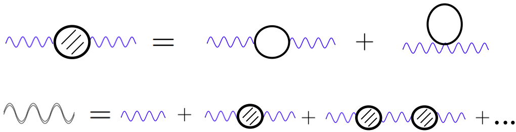
Figure 7: Top: The 1PI 1-loop correction to photon propagator, which consists of 2 diagrams. Bottom: In scalar QED, the exact photon propagator at order $\frac{1}{N_{f}}$is given by the sum of bubble diagrams.

4.1 Large-$N_{f}$ scalar QED on flat space

Quantum electrodynamics in different dimensions is a useful arena for studying strongly coupled gauge theories Pisarski:1984dj ; Appelquist:1986fd ; Appelquist:1988sr ; Roberts:1994dr . Considering the theory with $N_{f}$ scalar matter fields (sQED) at large $N_{f}$ and dimension $2<D<4$ the theory is asymptotically free and has an interesting phase structure. Consider $N_{f}$ scalar fields $\phi^{a}$ and a gauge field $A_{\mu}$, where the sQED Lagrangian with a quartic coupling is:

$$L=\frac{1}{4e^{2}}F_{\mu\nu}F^{\mu\nu}+|D_{\mu}\phi^{a}|^{2}+m^{2}|\phi^{a}|^{2}+\frac{\lambda}{2N_{f}}(\phi^{a}{\phi^{a}}^{*})^{2}$$ (59)

with the covariant derivative $D_{\mu}=\partial_{u}+iA_{\mu}$.This theory has an interesting phase structure with a broken and unbroken phase which are separated by a second order phase transition. Both these Higgs and Coulomb phases are gapless. In the Coulomb (unbroken) phase there is a massless photon and massive charged scalars $\phi^{a}$, whereas in the Higgs (broken) phase there are $2N_{f}-2$ massless Goldstone bosons and the photon becomes massive.

At large-$N_{f}$ it is useful to introduce a Hubbard-Stratonovich field $\sigma$, and the lagrangian Eq. 59 becomes:

$$L=\frac{1}{4e^{2}}F_{\mu\nu}F^{\mu\nu}+|D_{\mu}\phi^{a}|^{2}+m^{2}|\phi^{a}|^{2}+\frac{\sigma}{\sqrt{N_{f}}}\phi^{a}{\phi^{a}}^{*}-\frac{\sigma^{2}}{2\lambda}$$ (60)

The equation of motion for $\sigma$ is $\sigma=\frac{\lambda}{\sqrt{N}_{f}}$. At order $1/N_{f}$ the propagators of $\sigma$ and the photon $A_{\mu}$ can be computed exactly in the coupling constants $\lambda$ and $e$. The exact photon propagator is given by a resummation of the 1PI 2-point bubble diagrams, Fig. 7. In momentum space, this resummation of bubble diagrams just a geometric series:

$$\langle A_{\mu}(p)A_{\nu}(-p)\rangle=\frac{1}{N_{f}}\Big{[}\frac{\alpha}{p^{2}+\alpha B^{(1)}(p^{2},M^{2})}\Big{(}\delta_{\mu\nu}-\frac{p_{\mu}p_{\nu}}{p^{2}}\Big{)}+\zeta\frac{p_{\mu}p_{\nu}}{p^{4}}\Big{]}$$ (62)

where $\alpha\equiv N_{f}e^{2}$ and $\zeta=N_{f}\xi$. Where $B^{(1)}(p^{2},M^{2})$ is the 1-loop bubble function, which enters the 2-point function of currents:

$$\langle j_{\mu}(p)j_{\nu}(-p)\rangle=-N_{f}B^{(1)}(p^{2},M^{2})\Big{(}\delta_{\mu\nu}-\frac{p_{\mu}p_{\nu}}{p^{2}}\Big{)}$$ (63)

$B^{(1)}(p^{2},M^{2})$ is a simple function, easily computable as a 1-loop Feynman diagram. The $2\to 2$ scattering amplitude ${\phi^{a}}^{*}\phi^{b}\to{\phi^{c}}^{*}\phi^{d}$, will simply be the exchange diagram with exchange of the exact photon propagator Eq. 62 and Fig 8:

$$\mathcal{M}_{ab\to cd}=\frac{1}{N_{f}}\Big{(}\delta^{ab}\delta^{cd}\mathcal{M}(s,t)+\delta^{ac}\delta^{bd}\mathcal{M}(t,s)\Big{)}$$

$$\mathcal{M}(s,t)=\frac{\alpha(s-4M^{2}+2t)}{s-\alpha B^{(1)}(-s,M^{2})}\Big{(}\delta_{\mu\nu}-\frac{p_{\mu}p_{\nu}}{p^{2}}\Big{)}+\zeta\frac{p_{\mu}p_{\nu}}{p^{4}}$$ (64)

The poles of the scattering amplitude $\mathcal{M}(s,t)$ are thus determined by the zeros of the denominator, i.e $s-\alpha B^{(1)}(-s,M^{2})=0$.

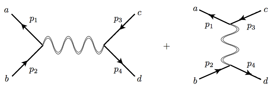
Figure 8: The two diagrams that contribute to the $2\to 2$ scattering amplitude $\phi^{a}\phi^{b}\to{\phi^{c}}^{*}\phi^{d}$ at order $\frac{1}{N_{f}}$. The letters $a,b,c,d$ denote $SU(N_{f})$ flavor indices.

4.2 Large-$N_{f}$ scalar QED on Anti de-Sitter space

We now consider the same model, but defined on $AdS_{d+1}$ instead of Eucledean space. We impose a Dirichlet boundary condition at the boundary of AdS, which gives rise to a global symmetry on the boundary. Just as in flat space, we would want to find the exact photon propagator at order $1/N_{f}$. In flat-space, working in momentum space enabled to resum bubble diagrams in a geometric series, Eq. 62. In AdS, the spectral representation can be viewed as the analogue of momentum space, and the spectral representation will enable us to resum bubble diagrams, just as in Fig. 7. For more details, see e.g Ankur:2023lum . The two-point function of the $U(1)$ conserved currents:

$$\langle j_{M}(X)j_{N}(Y)\rangle=-\int_{-\infty}^{\infty}d\nu B^{(1)}(\nu)\Omega^{(1)}_{\nu MN}(X,Y)$$ (65)

where $B^{(1)}(\nu)$ is the 1-loop bubble in the spectral representation, and $\Omega^{(1)}_{\nu MN}(X,Y)$ is the spin-1 AdS harmonic function. The sum of bubble diagrams becomes a geometric series in spectral space $\nu$, due to how $\Omega^{(1)}_{\nu MN}(X,Y)$ behaves under convolution. Using this fact, the exact photon propagator is, Fig. 7:

$$\langle A_{M}(X)A_{N}(Y)\rangle=\frac{1}{N_{f}}\int d\nu\frac{1}{\nu^{2}+(\frac{d}{2}-1)^{2}+\alpha B^{(1)}(\nu)}\Omega^{(1)}_{\nu MN}(X,Y)+\nabla^{M}_{X}\nabla^{N}_{y}L(u)$$

The 4-point boundary correlator is then obtained by attaching external legs, giving exchange Witten diagrams, with exchange of the exact propagator Eq. 4.2:

$$\langle\phi^{a}(P_{1})\phi^{b}{}^{*}(P_{2})\phi^{c}{}^{*}(P_{3})\phi^{d}(P_{4})\rangle|_{O(\frac{1}{N_{f}})}=\frac{1}{N_{f}}\Big{(}\delta^{ab}\delta^{cd}g_{12|34}+\delta^{ac}\delta^{bd}g_{13|24}\Big{)}$$ (67)

where

$$g_{12|34}=\int d^{d+1}Xd^{d+1}YK_{\Delta}(P_{1},X)i\nabla_{M}^{X}K_{\Delta}(P_{2},X)K_{\Delta}(P_{3},Y)i\nabla_{N}^{Y}K_{\Delta}(P_{4},Y)\langle A_{M}(X)A_{N}(Y)\rangle$$

Where $K_{\Delta}$ are bulk-to-boundary propagators. Using the split and spectral representation Eq. 4.2, the 4-point function becomes $g_{12|34}=A\times g_{l=1}(z,\bar{z})$:

$$g_{l=1}(z,\bar{z})=\int_{-\infty}^{\infty}d\nu\frac{1}{\nu^{2}+(\frac{d}{2}-1)^{2}+\alpha B^{(1)}(\nu)}\Upsilon_{\nu,l}^{\Delta}\mathcal{K}^{\Delta}_{\frac{d}{2}+i\nu,1}(z,\bar{z})$$ (69)

Now we will see an important case in which we can compute this integral and obtain the exact 4-point function $g_{l=1}(z,\bar{z})$ in terms of a different tree-level 4-point function.

4.2.1 Computing the 4-point correlator at the bulk conformal point

Focusing on $AdS_{3}$ ($d=2$), the 1-loop bubble is Ankur:2023lum :

$$B^{(1)}(\nu)=\frac{\nu}{16\pi(\nu^{2}+1)}\Big{(}-2(2\Delta-3)\nu+(\nu^{2}+4(\Delta-1)^{2})(i\psi(\Delta-\frac{i\nu}{2})-i\psi(\Delta+\frac{i\nu}{2}))\Big{)}$$

where $\psi(x)$ is the digamma function. In Ankur:2023lum , we showed strong proof that a bulk conformal point exists when $\Delta=1$ and $\alpha\to\infty$. Plugging $\Delta=1$, the 1-loop bubble function simplifies:

$$B^{(1)}(\nu)=\frac{\nu^{3}}{16(\nu^{2}+1)}\coth(\frac{\pi\nu}{2})=-\frac{i\nu^{3}}{16(\nu^{2}+1)}\frac{\Gamma_{1+\frac{i\nu}{2}}\Gamma_{-\frac{i\nu}{2}}}{\Gamma_{\frac{1}{2}-\frac{i\nu}{2}}\Gamma_{\frac{1}{2}+\frac{i\nu}{2}}}$$ (71)

Thus, Eq. 69 becomes at the bulk conformal point ($\alpha\to\infty$):

$$g_{l=1}(z,\bar{z})=\frac{1}{\alpha}\int d\nu\frac{1}{B^{(1)}(\nu))}\Upsilon_{\nu,l}^{\Delta}\mathcal{K}^{\Delta}_{\frac{d}{2}+i\nu,1}(z,\bar{z})$$ (72)

Using simple gamma function identities, we get that:

$$\Gamma_{1-\frac{i\nu}{2}}\Gamma_{1+\frac{i\nu}{2}}(B^{(1)}(\nu))^{-1}=\frac{32}{\nu^{2}}\times\Gamma_{\delta+\frac{-\frac{d}{2}-i\nu+1}{2}}\Gamma_{\delta+\frac{-\frac{d}{2}+i\nu+1}{2}}\Big{|}_{\delta=\frac{3}{2},d=2}$$ (73)

and hence

$$g_{l=1}(z,\bar{z})=\frac{32}{\alpha}\int d\nu\frac{1}{\nu^{2}}\Upsilon_{\nu,l=1}^{a_{p}=1,b_{p}=\frac{3}{2}}\mathcal{K}^{\Delta}_{\frac{d}{2}+i\nu,1}(z,\bar{z})$$ (74)

Therefore the latter gives a tree-level exchange diagram of a photon, with external scaling dimensions $\Delta_{1}=\Delta_{2}=1$ and $\Delta_{3}=\Delta_{4}=\frac{3}{2}$, see Fig. 9. We have thus managed to compute the non-perturbative 4-point function in terms of a tree-level exchange diagram.

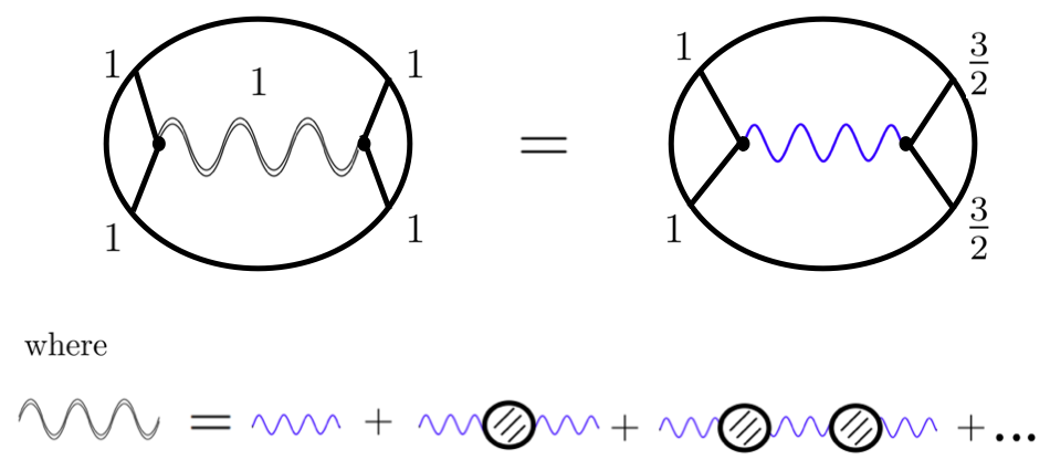
Figure 9: Showing Eq. 74. For scalar QED at the bulk conformal point (i.e $\Delta=1$ and $\alpha\to\infty$), the exact resummed 4-point function is equal to the tree-level photon exchange diagram on the right.

5 2-point bulk correlators

5.1 Bulk scalar 2-point correlators

The bulk-to-bulk propagator of a scalar field with scaling dimension $\Delta$ is (Eq. 1):

$$G_{\Delta}(x_{1},x_{2})=\frac{\Gamma_{\Delta}}{2\pi^{\frac{d}{2}}\Gamma_{\Delta-\frac{d}{2}+1}\sqrt{\zeta(\zeta+4)}}\zeta^{-\Delta}{}_{2}F_{1}(\Delta,\Delta-\frac{d-1}{2},2\Delta-d+1,-4\zeta^{-1})$$

Where $\zeta$ is the chordal distance squared. It will be convenient to express the hypergeometric function above in terms of a Legendre-Q function. Then the propagator can be written as:

$$G_{\Delta}(x_{1},x_{2})=e^{-\pi i\frac{d-1}{2}}\pi^{-\frac{d+1}{2}}(\zeta(\zeta+4))^{-\frac{d+1}{2}}Q^{\frac{d-1}{2}}_{\Delta-\frac{d+1}{2}}(1+\frac{\zeta}{2})$$ (76)

where $Q_{\mu}^{\nu}(x)$ is the associated Legendre function of the second kind. Thus the spectral representation of a general bulk 2-point function is (see Eq. 4):

$$g^{(2)}(\zeta)=\int_{-\infty}^{\infty}d\nu F_{\nu}\Omega_{\nu}(x_{1},x_{2})=\int_{-\infty}^{\infty}d\nu F_{\nu}i\nu G_{\frac{d}{2}+i\nu}$$

$$=\frac{1}{2\pi^{\frac{d}{2}}}\frac{\zeta^{-(\frac{d}{2})}}{\sqrt{\zeta(\zeta+4)}}\int_{-\infty}^{\infty}d\nu F_{\nu}\zeta^{-i\nu}{}_{2}F_{1}(\frac{d}{2}+i\nu,i\nu+\frac{1}{2},2i\nu+1,-4\zeta^{-1})$$ (77)

Or in terms of $Q$:

$$g^{(2)}(\zeta)=e^{-\pi i\frac{d-1}{2}}\pi^{-\frac{d+1}{2}}(\zeta(\zeta+4))^{-\frac{d+1}{2}}\int_{-\infty}^{\infty}d\nu F_{\nu}i\nu Q^{\frac{d-1}{2}}_{i\nu-\frac{1}{2}}(1+\frac{\zeta}{2})$$ (78)

5.2 A relation to the 4-point correlator

We will show in this subsection that the bulk 2-point correlator 78 is closely related to a specific boundary 4-point correlator. For $a=0$ and $b=\frac{1}{2}$, the scalar $J=0$ conformal block is given, for any $d$, by a hypergeometric function Dolan:2000ut :

$$\mathcal{K}^{\Delta_{i}}_{\frac{d}{2}+i\nu}(z,\bar{z})=\frac{1}{\sqrt{v}}\Big{(}\frac{1+\sqrt{v}}{2}\Big{)}^{1-\Delta}{}_{2}F_{1}\Big{(}\frac{\Delta-1}{2},\frac{\Delta}{2},\Delta+1-\frac{d}{2}:\frac{u}{(1+\sqrt{v})^{2}}\Big{)}$$ (79)

where the cross ratios are $u=z\bar{z}$ and $v=(1-z)(1-\bar{z})$. We can also write this in terms of the Legendre function:

$$\mathcal{K}^{\Delta_{i}}_{\frac{d}{2}+i\nu}(z,\bar{z})=\beta\times 4^{\Delta}\frac{\Gamma_{\Delta-\frac{d}{2}+1}}{\Gamma_{\Delta-1}}Q^{\frac{d-3}{2}}_{\Delta-\frac{d+1}{2}}(\sqrt{\frac{4}{X}})$$ (80)

where $X\equiv\frac{4u}{(1+\sqrt{v})^{2}}$ and $\beta\equiv\Big{(}2^{-\frac{d-1}{2}}e^{-\frac{d-3}{2}\pi i}(1-\frac{X}{4})^{-\frac{d-3}{4}}(\frac{X}{4})^{\frac{d-1}{4}}\Big{)}$. Additionally, the $\Upsilon$ factor of Eq. 21 for $a=0$, $b=\frac{1}{2}$ is:

$$\Upsilon_{\nu}^{\Delta_{i}}=\pi\Big{(}\frac{\Gamma_{a_{p}-\frac{d}{2}+\frac{\Delta}{2}}\Gamma_{b_{p}-\frac{d}{2}+\frac{\Delta}{2}}}{\Gamma_{1-a_{p}+\frac{\Delta}{2}}\Gamma_{1-b_{p}+\frac{\Delta}{2}}}\Big{)}2^{3-2\Delta}\frac{\Gamma_{\Delta-1}}{\Gamma_{\Delta-\frac{d}{2}}}$$ (81)

with $\Delta=\frac{d}{2}+i\nu$. Therefore

$$\Upsilon_{\nu}^{\Delta_{i}}\mathcal{K}^{\Delta_{i}}_{\frac{d}{2}+i\nu}(z,\bar{z})=8\pi\beta\Big{(}\frac{\Gamma_{a_{p}-\frac{d}{2}+\frac{\Delta}{2}}\Gamma_{b_{p}-\frac{d}{2}+\frac{\Delta}{2}}}{\Gamma_{1-a_{p}+\frac{\Delta}{2}}\Gamma_{1-b_{p}+\frac{\Delta}{2}}}\Big{)}(\Delta-\frac{d}{2})Q^{\frac{d-3}{2}}_{\Delta-\frac{d+1}{2}}(\sqrt{\frac{4}{X}})$$ (82)

Now we can make the factor in the brackets be 1, if we choose either $a_{p}=b_{p}=\frac{d+2}{4}$ or $b_{p}=1-a_{p}+\frac{d}{2}$. So we get:

$$\Upsilon_{\nu}^{\Delta_{i}}\mathcal{K}^{\Delta_{i}}_{\frac{d}{2}+i\nu}(z,\bar{z})=8\pi\beta(i\nu)Q^{\frac{d-3}{2}}_{i\nu-\frac{1}{2}}(\sqrt{\frac{4}{X}})$$ (83)

Plugging this in Eq. 23 gives:

$$dDisc[g_{l=0}]=\int_{-\infty}^{\infty}d\nu F_{\nu}\Upsilon_{\nu}^{\Delta_{i}}\mathcal{K}^{\Delta_{i}}_{\frac{d}{2}+i\nu}(z,\bar{z})=8\pi\beta\int_{-\infty}^{\infty}d\nu(i\nu)Q^{\frac{d-3}{2}}_{i\nu-\frac{1}{2}}(\sqrt{\frac{4}{X}})$$ (84)

Now we can use an identity for the Legendre function:

$$\mathcal{D}Q^{\frac{d-3}{2}}_{i\nu-\frac{1}{2}}(x)=Q^{\frac{d-1}{2}}_{i\nu-\frac{1}{2}}(x)$$ (85)

where the differential operator is defined as:

$$\mathcal{D}\equiv-(1-x^{2})^{\frac{d+1}{4}}\frac{d}{dx}(1-x^{2})^{\frac{d-1}{4}}$$ (86)

Therefore

$$\mathcal{D}[dDisc[g_{l=0}]]=\int_{-\infty}^{\infty}d\nu F_{\nu}\Upsilon_{\nu}^{\Delta_{i}}\mathcal{D}\mathcal{K}^{\Delta_{i}}_{\frac{d}{2}+i\nu}(z,\bar{z})=8\pi\beta\int_{-\infty}^{\infty}d\nu(i\nu)F_{\nu}Q^{\frac{d-1}{2}}_{i\nu-\frac{1}{2}}(\sqrt{\frac{4}{X}})$$ (87)

Comparing Eqs. 87 and 78, we get the relation:

$$\boxed{\mathcal{D}dDisc[g_{l=0}]]=c_{2}g^{(2)}(\zeta)\big{|}_{1+\frac{\zeta}{2}\to\sqrt{\frac{4}{X}})}}$$ (88)

where $c_{2}\equiv\frac{8\pi\beta}{e^{-\pi i\frac{d-1}{2}}\pi^{-\frac{d+1}{2}}(\zeta(\zeta+4))^{-\frac{d+1}{2}}}$. In other words, these 2-point and 4-point functions above have the same spectral integrals, and thus are directly related to each other. This identity is shown in Fig. 10.

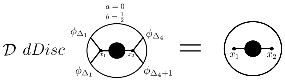
Figure 10: Relating the bulk two-point correlator on the right, to the $dDisc$ of the four-point function on the left. The black blob is the same on both sides, and is a general bulk two-point function.

5.3 Bulk spin-1 2-point correlators

5.3.1 spin-1 propagators

Consider a spin-1 massive Proca field with mass $m^{2}=(\Delta-1)(\Delta-d+1)$, the propagator $G_{\Delta,1}$ has two structures Costa:2014kfa :

$$G_{\Delta,1}\left(x_{1},x_{2};W_{1},W_{2}\right)=\left(W_{1}\cdot W_{2}\right)(G_{\Delta,1})_{0}\left(u\right)+\left(W_{1}\cdot x_{2}\right)\left(W_{2}\cdot x_{1}\right)(G_{\Delta,1})_{1}\left(u\right)~{},$$ (89)

where the coefficient functions $(G_{\Delta,1})_{0}(u)$ and $(G_{\Delta,1})_{1}(u)$ are

$$\begin{split}(G_{\Delta,1})_{0}\left(u\right)&=(d-\Delta)f_{1}(u)-\frac{1+u}{u}f_{2}(u),\\ (G_{\Delta,1})_{1}\left(u\right)&=\frac{(1+u)(d-\Delta)}{u(2+u)}f_{1}(u)-\frac{d+(1+u)^{2}}{u^{2}(2+u)}f_{2}(u)~{}.\end{split}$$ (90)

and where we defined the two hypergeometric functions:

$$\begin{split}f_{1}(u)&=\mathcal{N}(2u)^{-\Delta}{}_{2}F_{1}\left(\Delta,\frac{1-d+2\Delta}{2},1-d+2\Delta,-\frac{2}{u}\right)~{},\\ f_{2}(u)&=\mathcal{N}(2u)^{-\Delta}{}_{2}F_{1}\left(\Delta+1,\frac{1-d+2\Delta}{2},1-d+2\Delta,-\frac{2}{u}\right)~{},\\ &\mathcal{N}\equiv\frac{\Gamma(\Delta+1)}{2\pi^{d/2}(d-1-\Delta)(\Delta-1)\Gamma\left(\Delta+1-\frac{d}{2}\right)}~{}.\end{split}$$ (91)

In terms of the Legendre function, the coefficients can be written as follows:

$$(d-\Delta)f_{1}(u)=2^{\frac{-1-d}{2}}e^{-\pi i\frac{d-1}{2}}\pi^{-\frac{d+1}{2}}(u(u+2))^{-\frac{d-1}{4}}\frac{\nu^{2}+\frac{d^{2}}{4}}{\nu^{2}+(\frac{d}{2}-1)^{2}}Q^{\frac{d-1}{2}}_{i\nu-\frac{1}{2}}(1+u)$$

$$f_{2}(u)=-2^{\frac{-1-d}{2}}e^{-\pi i\frac{d+1}{2}}\pi^{-\frac{d+1}{2}}u(u(u+2))^{-\frac{d+1}{4}}\frac{1}{\nu^{2}+(\frac{d}{2}-1)^{2}}Q^{\frac{d+1}{2}}_{i\nu-\frac{1}{2}}(1+u)$$ (92)

where $u=\frac{\zeta}{2}$ and $\Delta=i\nu+\frac{d}{2}$.

5.3.2 2-point bulk correlators

If we have a spin-$1$ field in $AdS_{d+1}$. A general bulk 2-point function is:

$$g_{2}(x_{1},x_{2},W_{1},W_{2})=(W_{1}\cdot\nabla_{1})(W_{2}\cdot\nabla_{2}))\int_{-\infty}^{\infty}d\nu\tilde{F}^{L}(\nu)\Omega_{\nu,0}(x_{1},x_{2}:W_{1},W_{2})$$

$$+\int_{-\infty}^{\infty}d\nu\tilde{F}^{\perp}(\nu)\Omega_{\nu,1}(x_{1},x_{2}:W_{1},W_{2})$$ (93)

We focus on the transverse part in the second line. Now the AdS harmonic function is:

$$\Omega_{\nu,1}(x_{1},x_{2},W_{1},W_{2})=\frac{i\nu}{2\pi}\Big{(}G_{\frac{d}{2}+i\nu,1}(x_{1},x_{2},W_{1},W_{2})-G_{\frac{d}{2}-i\nu,1}(x_{1},x_{2},W_{1},W_{2})\Big{)}$$

Plugging this in the transverse part gives:

$$\int_{-\infty}^{\infty}d\nu\tilde{F}^{\perp}(\nu)\Omega_{\nu,1}=\frac{1}{2\pi}\int_{-\infty}^{\infty}d\nu\tilde{F}^{\perp}(\nu)i\nu G_{\frac{d}{2}+i\nu,1}=$$

$$\left(W_{1}\cdot W_{2}\right)\int_{-\infty}^{\infty}d\nu\tilde{F}^{\perp}(\nu)i\nu(G_{\frac{d}{2}+i\nu,1})_{0}\left(u\right)+\left(W_{1}\cdot x_{2}\right)\left(W_{2}\cdot x_{1}\right)\int_{-\infty}^{\infty}d\nu\tilde{F}^{\perp}(\nu)i\nu(G_{\frac{d}{2}+i\nu,1})_{1}\left(u\right)$$ (95)

This gives rise to two terms:

$$\int d\nu\tilde{F}(\nu)i\nu(-i\nu+\frac{d}{2})f_{1}(u)$$

$$=2^{\frac{-1-d}{2}}e^{-\pi i\frac{d-1}{2}}\pi^{-\frac{d+1}{2}}(u(u+2))^{-\frac{d-1}{4}}\int d\nu F_{\nu}i\nu\frac{\nu^{2}+\frac{d^{2}}{4}}{\nu^{2}+(\frac{d}{2}-1)^{2}}Q^{\frac{d-1}{2}}_{i\nu-\frac{1}{2}}(1+u)$$

$$=2^{\frac{-1-d}{2}}e^{-\pi i\frac{d-1}{2}}\pi^{-\frac{d+1}{2}}(u(u+2))^{-\frac{d-1}{4}}\int d\nu F_{\nu}i\nu\Big{[}1+\frac{d-1}{\nu^{2}+(\frac{d}{2}-1)^{2}}\Big{]}Q^{\frac{d-1}{2}}_{i\nu-\frac{1}{2}}(1+u)$$ (96)

and

$$\int d\nu F_{\nu}i\nu f_{2}(u)$$

$$=-2^{\frac{-1-d}{2}}e^{-\pi i\frac{d+1}{2}}\pi^{-\frac{d+1}{2}}u(u(u+2))^{-\frac{d+1}{4}}\int d\nu F_{\nu}i\nu\frac{1}{\nu^{2}+(\frac{d}{2}-1)^{2}}Q^{\frac{d+1}{2}}_{i\nu-\frac{1}{2}}(1+u)$$ (97)

Using

$$\widehat{\mathcal{D}}Q^{\frac{d-1}{2}}_{i\nu-\frac{1}{2}}(x)=Q^{\frac{d+1}{2}}_{i\nu-\frac{1}{2}}(x)$$ (98)

with

$$\widehat{\mathcal{D}}\equiv-(1-x^{2})^{\frac{d+3}{4}}\frac{d}{dx}(1-x^{2})^{\frac{d+1}{4}}$$ (99)

gives:

$$\int d\nu F_{\nu}i\nu f_{2}(u)$$

$$=-2^{\frac{-1-d}{2}}e^{-\pi i\frac{d+1}{2}}\pi^{-\frac{d+1}{2}}u(u(u+2))^{-\frac{d+1}{4}}\widehat{\mathcal{D}}\int d\nu F_{\nu}i\nu\frac{1}{\nu^{2}+(\frac{d}{2}-1)^{2}}Q^{\frac{d-1}{2}}_{i\nu-\frac{1}{2}}(1+u)$$ (100)

These two integrals can be easily related to scalar bulk 2-point integrals given in Eq. 78. In particular to get the integral in Eq. 5.3.2, one simply attaches a free propagator. To get the intergral in Eq. 5.3.2, one attaches a free propagator and acts with the derivative operator $2D_{z,\bar{z}}$ with $l=0$, see Eq. 39. Therefore the spin-1 bulk 2-point functions are closely related to spin-0 ones.

6 The 4-point 1-loop bubble diagram

In this subsection we compute various 4-point 1-loop bubble diagrams. What we are after is the dependence of the 4-point function on the cross-ratios $z$ and $\bar{z}$. Therefore we will drop overall factors which do not depend on the cross-ratios. Let us look at the 1-loop scalar bubble in the spectral representation. The bubble $\tilde{B}$ has single poles:

$$\tilde{B}(\nu)\overset{\frac{d}{2}+i\nu\sim 2\Delta+2n}{\sim}\widehat{A}_{\Delta}\Lambda_{n,\Delta}\times\frac{1}{\frac{d}{2}+i\nu-(2\Delta+2n)}$$ (101)

where we defined

$$\Lambda_{n,\Delta}\equiv\frac{\Gamma_{\frac{d}{2}+n}\Gamma_{n+\Delta}\Gamma_{\frac{1}{2}-\frac{d}{2}+n+\Delta}\Gamma_{2\Delta+n-\frac{d}{2}}}{\Gamma_{n+1}\Gamma_{n+\Delta+1-\frac{d}{2}}\Gamma_{n+\Delta+\frac{1}{2}}\Gamma_{1-d+n+2\Delta}}$$ (102)

Therefore from Eq. 26

$$dDisc[g_{4}(z,\bar{z})]\Big{|}_{1-loop}=\widehat{A}_{\Delta,l}\sum^{\infty}_{n=0}\Lambda_{n,\Delta}\times\Upsilon_{\nu,l=0}^{\Delta_{i}}\mathcal{K}^{\Delta_{i}}_{\frac{d}{2}+i\nu,l=0}(z,\bar{z})\Big{|}_{i\nu+\frac{d}{2}\to 2\Delta+2n}$$ (103)

6.1 Scalar bubble diagram, odd $d$

$\bullet$ $d=3$

The poles of the 1-loop bubble in $d=3$ and $l=0$ are, see Eq. 101:

$$2\tilde{B}_{\nu}\sim-\frac{1}{\frac{d}{2}+i\nu-(2\Delta+2n)}\sqrt{\pi}2^{1-4\Delta}\Gamma_{2\Delta}\Gamma_{2\Delta+1}\frac{\Gamma_{n+\frac{3}{2}}\Gamma^{2}_{\Delta+n+\frac{1}{2}}\Gamma_{2\Delta+n+\frac{1}{2}}}{\Gamma_{n+1}\Gamma^{2}_{\Delta+n+1}\Gamma_{n+2\Delta}}$$ (104)

Thus for $\Delta=1,2$, the residue is constant:

$$2\tilde{B}_{\nu}\sim-\frac{\frac{4}{\sqrt{\pi}}}{\frac{d}{2}+i\nu-(2\Delta+2n)}$$ (105)

Using Eq. 103, 21 and 25, we see that for $b_{p}=\Delta$ and $\Delta=1,2$ we have

$$dDisc[g_{l=0}]=Disc_{a_{p}}[g_{l=0}(z,\bar{z})]\Big{|}_{Contact}$$ (106)

Thus, this family of 1-loop diagrams can be computed via the tree-level contact diagram. This is schematially shown in Fig. 11.

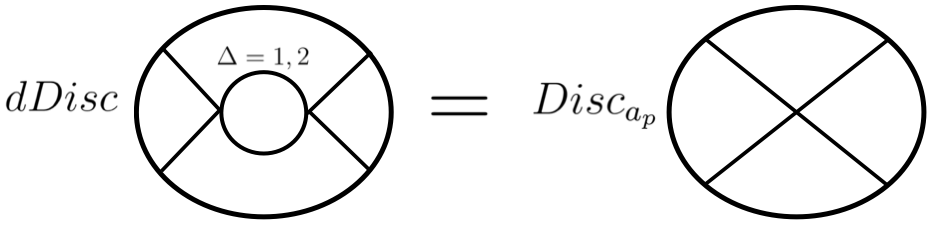
Figure 11: Showing the relation of Eq. 106 between the 4-point 1-loop diagram and contact diagrams for $d=3$ and $\Delta=1,2$. Similar relations exist in $d=5$ with $\Delta=3,4$, shown in Eq. 108-109.

$\bullet$ $d=5$

In $d=5$ and When $\Delta=3,4$, the residue is :

$$2\tilde{B}_{\nu}\sim-\frac{\frac{1}{3\sqrt{\pi}}(2n+3)(2n+4)}{\frac{d}{2}+i\nu-(2\Delta+2n)}\ \ \ \ \ \ ,\ \ \ \ \ \ \ 2\tilde{B}_{\nu}\sim-\frac{\frac{1}{3\sqrt{\pi}}(2n+2)(2n+9)}{\frac{d}{2}+i\nu-(2\Delta+2n)}$$ (107)

Using Eq. 39, and after choosing $b_{p}=\Delta$, we get a relation between the 1-loop and contact diagram:

$$dDisc[g_{l=0}]\Big{|}_{\Delta=3}=(2D_{z,\bar{z}}+6)Disc_{a_{p}}[g_{l=0}(z,\bar{z})]\Big{|}_{Contact}$$ (108)

and

$$dDisc[g_{l=0}\Big{|}_{\Delta=4}=(2D_{z,\bar{z}}-6)Disc_{a_{p}}[g_{l=0}(z,\bar{z})]\Big{|}_{Contact}$$ (109)

6.2 Fermionic bubble diagram

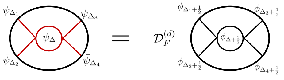
Figure 12: Showing a relation between the 4-point 1-loop diagrams of fermions and scalars in $d=1,2$. The relations are given in Eqs. 111 and 113.

In section 6 of Carmi:2018qzm , we studied the 1-loop fermionic bubble diagram in $d=1,2$. In the current subsection we relate the 4-point 1-loop fermionic bubble to the scalar bubble.

$\bullet$ $d=1$

In $d=1$ the poles of the 1-loop fermion bubble are Carmi:2018qzm :

$$2\tilde{B}^{(F)}_{\nu}\sim-\frac{1}{\frac{d}{2}+i\nu-(2\Delta+2n+1)}\sqrt{\pi}2^{1-4\Delta}\Gamma_{2\Delta}\Gamma_{2\Delta+1}\frac{\Gamma_{n+\frac{3}{2}}\Gamma^{2}_{\Delta+n+\frac{1}{2}}\Gamma_{2\Delta+n+\frac{1}{2}}}{\Gamma_{n+1}\Gamma^{2}_{\Delta+n+1}\Gamma_{n+2\Delta}}$$ (110)

The scalar bubble is given in Eq. 101. Thus, attaching bulk-to-boundary propagators, one can see that the 4-point 1-loop fermion bubble is directly related to the scalar 1-loop bubble with external scalars (see Fig. 12):

$$\boxed{g_{F}^{(\Delta_{i},\Delta)}(z,\bar{z})=\mathcal{D}_{F}^{(d=1)}g_{B}^{(\Delta_{i}+\frac{1}{2},\Delta+\frac{1}{2})}(z,\bar{z})}$$ (111)

where we defined the differential operator $\mathcal{D}_{F}^{(d=1)}\equiv c_{\Delta}(2D_{z,\bar{z}}-2\Delta(2\Delta-1))$.

$\bullet$ $d=2$

In $d=2$ the poles of the 1-loop fermion bubble is Carmi:2018qzm :

$$2\tilde{B}_{\nu}^{(F)}\sim-\frac{1}{\frac{d}{2}+i\nu-(2\Delta+2n+1)}\frac{(n+1)(2\Delta+n-1)}{n+\Delta}$$ (112)

Thus, attaching bulk-to-boundary propagators, the 4-point 1-loop fermion bubble is directly related to the scalar 1-loop bubble with external scalars (see Fig. 12):

$$\boxed{g_{F}^{(\Delta_{i},\Delta)}(z,\bar{z})=\mathcal{D}_{F}^{(d=2)}g_{B}^{(\Delta_{i}+\frac{1}{2},\Delta+\frac{1}{2})}(z,\bar{z})}$$ (113)

where we defined the differential operator $\mathcal{D}_{F}^{(d=2)}\equiv\tilde{c}_{\Delta}(2D_{z,\bar{z}}-4\Delta^{2}+8\Delta-3)$.

7 4-point ladder diagrams

In this section we discuss the computation of ladder diagrams with spinning fields, and in particular for gauge theories. This extends the results of Carmi:2021dsn , in which we derived the spectral representation for ladder diagrams of scalar fields in AdS. We consider a theory with a cubic interaction of scalar field with a spin-$L$ field. The expression for the 0-loop ladder diagram, which is just the tree-level exchange diagram Fig. 13-Left:

$$\mathcal{M}^{(0)}=\mathcal{M}^{3214}_{5,exch}=\sum^{\infty}_{J=0}\int_{-\infty}^{\infty}\frac{d\mu}{2\pi i}\ R^{1234}_{\mathcal{O}_{5},\mathcal{O}_{\mu,J}}\ \Psi^{1234}_{\mu,J}$$ (114)

See Eq. 139. We can now add a rung to the ladder, giving 1-loop the box diagram Fig 13-Middle. This diagram can then be computed by gluing two tree-level diagrams, schematically:

$$\mathcal{M}^{(1)}=\mathcal{M}_{Box}=\mathcal{M}^{621\tilde{\underline{8}}}_{5,exch}\otimes\mathcal{M}^{3\tilde{\underline{6}}\underline{8}4}_{7,exch}$$ (115)

And the ladder diagram at $N$-loops is obtained by gluing $N$ tree-level diagrams:

$$\mathcal{M}^{(N)}=\mathcal{M}_{1,exch.}\otimes\mathcal{M}_{2,exch.}\otimes\cdots\otimes\mathcal{M}_{N-1,exch.}\otimes\mathcal{M}_{N,exch.}$$ (116)

This procedure yields, for the $N$-loop ladder diagrams, the expression for the OPE function:

$$\mathcal{M}^{(N)}=\sum^{\infty}_{J_{5}=0}\int_{-\infty}^{\infty}\frac{d\mu_{5}}{2\pi i}C^{(N)}_{\mu_{5},J_{5}}\Psi^{1234}_{\mu_{5},J_{5}}$$ (117)

where $C^{(N)}_{\mu_{5},J_{5}}$is the respective OPE function at $N$-loops. From Eq. 139 we have for the tree-level exchange diagram:

$$C^{(0)}_{\mu,J}=R^{{\color[rgb]{1,0,0}1},{\color[rgb]{1,0,0}2},{\color[rgb]{1,0,0}3},{\color[rgb]{1,0,0}4}}_{\mu,J}$$ (118)

At 1-loop we have:

$$C^{(1)}_{\mu,J}=B_{\mu,J}\int_{-\infty}^{\infty}\bigg{(}\prod_{i=6,8}\frac{d\nu_{i}\nu_{i}^{2}}{\nu_{i}^{2}+(\Delta_{i}-\frac{d}{2})^{2}}\bigg{)}R^{{\color[rgb]{1,0,0}1},{\color[rgb]{1,0,0}2},6,8}_{\mu,J}R^{\tilde{8},\tilde{6},{\color[rgb]{1,0,0}3},{\color[rgb]{1,0,0}4}}_{\mu,J}$$ (119)

We get the following expression for the $N$-loop OPE function of the ladder diagram:

$$\boxed{C^{(N-loop)}_{\mu,J}=\big{(}B_{\mu,J}\big{)}^{N}\int_{-\infty}^{\infty}\bigg{(}\prod_{horiz.}\frac{d\nu_{i}\nu_{i}^{2}}{\nu_{i}^{2}+(\Delta_{i}-\frac{d}{2})^{2}}\bigg{)}\prod_{vertical}R_{\mu,J}}$$ (120)

Where we defined the product:

$$\prod_{vertical}R_{\mu,J}=R^{{\color[rgb]{1,0,0}1},{\color[rgb]{1,0,0}2},A_{1},B_{1}}_{\mu,J}R^{\tilde{B}_{1},\tilde{A}_{1},A_{2},B_{2}}_{\mu,J}R^{\tilde{B}_{2},\tilde{A}_{2},A_{3},B_{3}}_{\mu,J}\ \ \cdots\ R^{\tilde{B}_{\hat{N}-1},\tilde{A}_{\hat{N}-1},A_{\hat{N}},B_{\hat{N}}}_{\ \mu,J}R^{\tilde{B}_{\hat{N}},\tilde{A}_{\hat{N}},{\color[rgb]{1,0,0}3},{\color[rgb]{1,0,0}4}}_{\mu,J}$$ (121)

In appendix A we derive Eq. 120 explicitly for the 2-loop case. The same type of derivation extends to $N$-loops, giving Eq. 120.

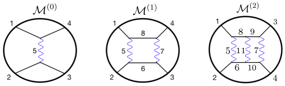
Figure 13: Four-point ladder diagrams for exchanges of a spin-$L$ field. Left: The 0-loop ladder, tree level exchange. Middle: The 1-loop ladder, i.e the box diagram. Right: The ladder diagram at 2-loops.

8 Discussion

In this work we used the spectral representation as a tool to compute various families of loop diagrams in anti de-Sitter space, including blob diagrams and ladder diagrams. The spectral representation makes various identities explicit, enabling to related loop Witten diagrams to lower loop diagrams. We saw that it was often simpler to compute the double-discontinuity of a diagram. The conformal dispersion relation Carmi:2019cub , and it’s generalization to mixed correlators carmi3 , can then be used to reconstruct the full 4-point correlator.

The spectral representation has recently been used for de-Sitter space, and it would be interesting to import our AdS methods to compute blob diagrams in deSitter. The $O(N)$ model at large-$N$ has recently been studied in de Sitter space DiPietro:2023inn , can one extend these computations for the case of the fermionic Gross-Neveu model and to large-$N_{f}$ QED on deSitter. We also leave for future work the computation of loops of gluons and gravitons in AdS and dS.

In order to make progress on analytic loop computations of diagrams in AdS, it can be useful to consider some simplifying limits, such as the flat-space limit of AdS diagrams. Conformal blocks simplify in the large $d$ limit, which might enable to perform analytical computations using the spectral representation. Another simplifying limit is the diagonal limit $\bar{z}=z$, which is essentially a 1d limit.

Acknowledgements: I thank Lorenzo Di Pietro and Ankur Ankur for discussions. This work was supported by the Israeli Science Foundation (ISF) grant number 1487/21, and by the MOST NSF/BSF physics grant number 2022726.

Appendix A Ladder diagrams

A.1 Ladder diagram at tree-level

The conformal partial wave (CPW) $\Psi$ in the s-channel is related to the CPW in the t-channel via, see Liu:2018jhs ; Meltzer:2019nbs :

$$\Psi^{3214}_{\mu_{6},l_{6}}(x_{i})=\sum^{\infty}_{J=0}\int_{-\infty}^{\infty}\frac{d\mu}{2\pi i}\left\{\begin{array}[]{c}\ \mathcal{O}_{1},\mathcal{O}_{2},\mathcal{O}_{\mu_{6},l_{6}}\\ \mathcal{O}_{3},\mathcal{O}_{4},\mathcal{O}_{\mu,J}\end{array}\right\}\frac{1}{n_{\mathcal{O}_{\mu,J}}}\Psi^{1234}_{\mu,J}$$ (124)

Where the factor in the brackets is a 6J symbol.

$$\left\{\begin{array}[]{c}\ \mathcal{O}_{1},\mathcal{O}_{2},\mathcal{O}_{\mu_{6},l_{6}}\\ \mathcal{O}_{3},\mathcal{O}_{4},\mathcal{O}_{\mu,J}\end{array}\right\}=K^{14}_{\tilde{6}}\left(\begin{array}[]{c}\ \mathcal{O}_{1},\mathcal{O}_{2},\mathcal{O}_{\mu_{6},l_{6}}\\ \mathcal{O}_{3},\mathcal{O}_{4},\mathcal{O}_{\mu,J}\end{array}\right)+K^{23}_{6}\left(\begin{array}[]{c}\ \mathcal{O}_{1},\mathcal{O}_{2},\tilde{\mathcal{O}}_{\mu_{6},l_{6}}\\ \mathcal{O}_{3},\mathcal{O}_{4},\mathcal{O}_{\mu,J}\end{array}\right)$$ (131)

Now consider the tree-level exchange diagram of a spin-$L$ field in AdS (Fig. 13-Left). Expanded in the direct $s$-channel partial waves, we have Costa:2014kfa :

$$\mathcal{M}^{3214}_{5,exch}=A\sum_{l_{5}=0}^{L}\int_{-\infty}^{\infty}d\mu_{5}b_{l_{5}}(\mu_{5})\Psi^{3214}_{\mu_{5},l_{5}}$$ (132)

where $A$ is defined in Eq. 18. Using Eq. 124 gives an expansion in terms of the $t$-channel CPWs:

$$\mathcal{M}^{3214}_{5,exch}=A\sum^{\infty}_{J=0}\int\frac{d\mu}{2\pi i}\sum_{l_{5}=0}^{L}\int d\mu_{5}b_{l_{5}}(\mu_{5})K^{14}_{\tilde{5}}\left(\begin{array}[]{c}\mathcal{O}_{1},\mathcal{O}_{2},\mathcal{O}_{5,l_{5}}\\ \mathcal{O}_{3},\mathcal{O}_{4},\mathcal{O}_{\mu,J}\end{array}\right)\frac{1}{n_{\mathcal{O}_{\mu,J}}}\Psi^{1234}_{\mu,J}$$ (135)

In the integrand above, we can define the following factor:

$$R^{1234}_{\mu,J}\equiv\sum_{l_{5}=0}^{L}\int_{-\infty}^{\infty}d\mu_{5}b_{l_{5}}(\nu)K^{14}_{\tilde{5}}\left(\begin{array}[]{c}\mathcal{O}_{1},\mathcal{O}_{2},\mathcal{O}_{5,l_{5}}\\ \mathcal{O}_{3},\mathcal{O}_{4},\mathcal{O}_{\mu,J}\end{array}\right)\frac{1}{n_{\mathcal{O}_{\mu,J}}}$$ (138)

Therefore Eq. 135 gives:

$$\mathcal{M}^{(0)}=\mathcal{M}^{3214}_{5,exch}=\sum^{\infty}_{J=0}\int_{-\infty}^{\infty}\frac{d\mu}{2\pi i}\ R^{1234}_{\mu,J}\ \Psi^{1234}_{\mu,J}$$ (139)

This is the expression for the tree-level 4-point ladder diagram, Fig. 13-Left, expanded in the cross-channel conformal partial waves. $C^{(0)}_{\mu,J}=R^{1234}_{\mu,J}$ is the ”OPE function” for this diagram Caron-Huot:2017vep .

A.2 Ladder diagram at 2-loop

We show in this section the details of the calculation of the 2-loop ladder diagram, which will then then easily generalise to $N$-loops. In particular, we will derive the following conformal partial wave expansion:

$$\mathcal{M}^{(2)}=\sum^{\infty}_{J_{5}=0}\int_{-\infty}^{\infty}\frac{d\mu_{5}}{2\pi i}C^{(2)}_{\mu_{5},J_{5}}\Psi^{1234}_{\mu_{5},J_{5}}$$ (140)

and will explicitly derive the OPE function $C^{(2)}_{\mu_{5},J_{5}}$.

The 4-point ladder diagram at two-loops is given by (see Fig. 13-Right):

$$\mathcal{M}^{(2)}=\int d^{d+1}x_{1}\cdots d^{d+1}x_{6}\ \nabla^{L}_{1}\ K_{\Delta_{1}}(P_{1},x_{1})\nabla^{L}_{2}\nabla_{x_{2}}K_{\Delta_{2}}(P_{2},x_{2})$$

$$\nabla^{L}_{3}K_{\Delta_{3}}(P_{3},x_{3})\nabla^{L}_{4}K_{\Delta_{4}}(P_{4},x_{4})$$

$$G_{\Delta_{5},L}(x_{1},x_{2})G_{\Delta_{7},L}(x_{3},x_{4})\ G_{\Delta_{11},L}(x_{5},x_{6})$$

$$\nabla^{L}_{5}G_{\Delta_{8}}(x_{1},x_{5})\ \nabla^{L}_{6}G_{\Delta_{6}}(x_{2},x_{6})\ G_{\Delta_{9}}(x_{5},x_{3})\ G_{\Delta_{10}}(x_{6},x_{4})~{}.$$ (141)

Here we defined $\nabla^{L}_{i}\equiv(K_{i}\cdot\nabla_{x_{i}})^{L}$. Now we will use the spectral representation for the four bulk-to-bulk propagators on the last line above:

$$\nabla^{L}_{5}G_{\Delta_{8}}(x_{1},x_{5})=\nabla^{L}_{5}\int_{-\infty}^{\infty}d\nu_{8}\frac{1}{\nu_{8}^{2}+(\Delta_{8}-\frac{d}{2})^{2}}\Omega_{\nu_{8}}(x_{1},x_{5})$$

$$\nabla^{L}_{6}G_{\Delta_{6}}(x_{2},x_{6})=\nabla^{L}_{6}\int_{-\infty}^{\infty}d\nu_{6}\frac{1}{\nu_{6}^{2}+(\Delta_{6}-\frac{d}{2})^{2}}\Omega_{\nu_{6}}(x_{2},x_{6})$$ (142)

and

$$G_{\Delta_{9}}(x_{5},x_{3})=\int_{-\infty}^{\infty}d\nu_{9}\frac{1}{\nu_{9}^{2}+(\Delta_{9}-\frac{d}{2})^{2}}\Omega_{\nu_{9}}(x_{5},x_{3})$$

$$G_{\Delta_{10}}(x_{6},x_{4})=\int_{-\infty}^{\infty}d\nu_{10}\frac{1}{\nu_{10}^{2}+(\Delta_{10}-\frac{d}{2})^{2}}\Omega_{\nu_{10}}(x_{6},x_{4})$$ (143)

Now we use the split representation for the AdS harmonic functions:

$$\Omega_{\nu_{8}}(x_{1},x_{5})=\frac{\nu_{8}^{2}}{\pi}\int d^{d}Q_{8}K_{\frac{d}{2}-i\nu_{8}}(Q_{8},x_{1})K_{\frac{d}{2}+i\nu_{8}}(Q_{8},x_{5})$$

$$\Omega_{\nu_{6}}(x_{2},x_{6})=\frac{\nu_{6}^{2}}{\pi}\int d^{d}Q_{6}K_{\frac{d}{2}+i\nu_{6}}(Q_{6},x_{2})K_{\frac{d}{2}-i\nu_{6}}(Q_{6},x_{6})$$

$$\Omega_{\nu_{9}}(x_{5},x_{3})=\frac{\nu_{9}^{2}}{\pi}\int d^{d}Q_{9}K_{\frac{d}{2}-i\nu_{9}}(Q_{9},x_{5})K_{\frac{d}{2}+i\nu_{9}}(Q_{9},x_{3})$$

$$\Omega_{\nu_{10}}(x_{6},x_{4})=\frac{\nu_{10}^{2}}{\pi}\int d^{d}Q_{10}K_{\frac{d}{2}-i\nu_{10}}(Q_{10},x_{6})K_{\frac{d}{2}+i\nu_{10}}(Q_{10},x_{4})$$ (144)

Here the $Q_{j}$ are points on the boundary. Thus Eq. A.2 becomes:

$$\mathcal{M}^{(2)}=\frac{1}{\pi^{4}}\prod_{i=6,8,9,10}\int_{-\infty}^{\infty}d\nu_{i}\int d^{d}Q_{i}\frac{\nu_{i}^{2}}{\nu_{i}^{2}+(\Delta_{i}-\frac{d}{2})^{2}}$$

$$\int d^{d+1}x_{1}d^{d+1}x_{2}\ \nabla^{L}_{1}K_{\Delta_{1}}(P_{1},x_{1})\nabla^{L}_{2}K_{\Delta_{2}}(P_{2},x_{2})K_{\frac{d}{2}-i\nu_{8}}(Q_{8},x_{1})K_{\frac{d}{2}+i\nu_{6}}(Q_{6},x_{2})G_{\Delta_{5},L}(x_{1},x_{2})$$

$$\int d^{d+1}x_{3}d^{d+1}x_{4}\ \nabla^{L}_{3}K_{\Delta_{3}}(P_{3},x_{3})\nabla^{L}_{4}K_{\Delta_{4}}(P_{4},x_{4})K_{\frac{d}{2}+i\nu_{9}}(Q_{9},x_{3})K_{\frac{d}{2}+i\nu_{10}}(Q_{10},x_{4})G_{\Delta_{7},L}(x_{3},x_{4})$$

$$\int d^{d+1}x_{5}d^{d+1}x_{6}\ \nabla^{L}_{5}K_{\frac{d}{2}+i\nu_{8}}(Q_{8},x_{5})\nabla^{L}_{6}K_{\frac{d}{2}-i\nu_{6}}(Q_{6},x_{6})K_{\frac{d}{2}-i\nu_{10}}(Q_{10},x_{6})K_{\frac{d}{2}-i\nu_{9}}(Q_{9},x_{5})G_{\Delta_{11},L}(x_{5},x_{6})$$ (145)

We see that we have a product of three tree-level exchange diagrams:

$$\mathcal{M}^{(2)}=\frac{1}{\pi^{4}}\prod_{i=6,8,9,10}\int_{-\infty}^{\infty}d\nu_{i}\int d^{d}Q_{i}\frac{\nu_{i}^{2}}{\nu_{i}^{2}+(\Delta_{i}-\frac{d}{2})^{2}}\ \ \mathcal{M}^{6,2,1,\tilde{8}}_{5,exch}\otimes\mathcal{M}^{8,\tilde{6},\tilde{10},\tilde{9}}_{11,exch}\otimes\mathcal{M}^{3,9,10,4}_{7,exch}$$ (146)

Now we use Eq. 139, to expand the tree-level diagrams above in the crossed channel:

$$\mathcal{M}^{621\tilde{8}}_{\mathcal{O}_{5},exch}=\sum^{\infty}_{J_{5}=0}\int\frac{d\mu_{5}}{2\pi i}\ R^{{\color[rgb]{1,0,0}12}6\tilde{8}}_{\mathcal{O}_{5},O_{\mu_{5},J_{5}}}\ \Psi^{126\tilde{8}}_{\mu_{5},J_{5}}$$

$$\mathcal{M}^{3,9,10,4}_{\mathcal{O}_{7},exch}=\sum^{\infty}_{J_{7}=0}\int\frac{d\mu_{7}}{2\pi i}\ R^{10,9,{\color[rgb]{1,0,0}34}}_{\mathcal{O}_{7},O_{\mu_{7},J_{7}}}\ \Psi^{10,9,3,4}_{\mu_{7},J_{7}}$$

$$\mathcal{M}^{8,\tilde{6},\tilde{10},\tilde{9}}_{\mathcal{O}_{11},exch}=\sum^{\infty}_{J_{11}=0}\int\frac{d\mu_{11}}{2\pi i}\ R^{\tilde{6},8,\tilde{9},\tilde{10}}_{\mathcal{O}_{11},O_{\mu_{11},J_{11}}}\ \Psi^{\tilde{6},8,\tilde{9},\tilde{10}}_{\mu_{11},J_{11}}$$ (147)

Thus,

$$\mathcal{M}^{(2)}=\frac{1}{\pi^{4}}\int_{-\infty}^{\infty}\bigg{(}\prod_{i=6,8,9,10}d\nu_{i}\frac{\nu_{i}^{2}}{\nu_{i}^{2}+(\Delta_{i}-\frac{d}{2})^{2}}\bigg{)}\sum^{\infty}_{J_{5}=0}\sum^{\infty}_{J_{7}=0}\sum^{\infty}_{J_{11}=0}\int\frac{d\mu_{5}}{2\pi i}\int\frac{d\mu_{7}}{2\pi i}\int\frac{d\mu_{11}}{2\pi i}$$

$$R^{{\color[rgb]{1,0,0}12}6\tilde{8}}_{\mathcal{O}_{5},O_{\mu_{5},J_{5}}}R^{\tilde{6},8,\tilde{9},\tilde{10}}_{\mathcal{O}_{11},O_{\mu_{11},J_{11}}}R^{10,9,{\color[rgb]{1,0,0}34}}_{\mathcal{O}_{7},O_{\mu_{7},J_{7}}}\times\int d^{d}Q_{8}d^{d}Q_{6}\int d^{d}Q_{9}d^{d}Q_{10}\Psi^{126\tilde{8}}_{\mu_{5},J_{5}}\Psi^{10,9,3,4}_{\mu_{7},J_{7}}\Psi^{\tilde{6},8,\tilde{9},\tilde{10}}_{\mu_{11},J_{11}}$$ (148)

The CPWs above have a shadow representation:

$$\Psi^{126\tilde{8}}_{\mu_{5},J_{5}}=\int d^{d}P_{0}\langle O(P_{1})O(P_{2})O_{\mu_{5},J_{5}}(P_{0})\rangle\langle\tilde{O}_{\mu_{5},J_{5}}(P_{0})\tilde{O}(Q_{8})O(Q_{6})\rangle$$

$$\Psi^{10,9,3,4}_{\mu_{7},J_{7}}=\!\!\int d^{d}P_{0}^{\prime}\langle O(Q_{10})O(Q_{9})O_{\mu_{7},J_{7}}(P_{0}^{\prime})\rangle\langle\tilde{O}_{\mu_{7},J_{7}}(P_{0}^{\prime})O(P_{3})O(P_{4})\rangle$$

$$\Psi^{\tilde{6},8,\tilde{9},\tilde{10}}_{\mu_{11},J_{11}}=\!\!\int d^{d}P_{0}^{\prime\prime}\langle\tilde{O}(Q_{6})O(Q_{8})O_{\mu_{11},J_{11}}(P_{0}^{\prime\prime})\rangle\langle\tilde{O}_{\mu_{11},J_{11}}(P_{0}^{\prime\prime})\tilde{O}(Q_{9})\tilde{O}(Q_{10})\rangle$$ (149)

Now we plug Eq. A.2 in Eq. A.2, and we can do the $Q_{6}$, $Q_{8}$ integrals:

$$\int d^{d}Q_{8}d^{d}Q_{6}\langle\tilde{O}_{\mu_{5},J_{5}}(P_{0})\tilde{O}(Q_{8})O(Q_{6})\rangle\langle O(Q_{8})\tilde{O}(Q_{6})O_{\mu_{11},J_{11}}(P_{0}^{\prime\prime})\rangle$$

$$=B_{\mu_{5},J_{5}}\delta_{P_{0},P_{0}^{\prime\prime}}\delta_{\mu_{5},\mu_{11}}\delta_{J_{5},J_{11}}~{}.$$ (150)

and the $Q_{9}$, $Q_{10}$ integrals as follows:

$$\int d^{d}Q_{9}d^{d}Q_{10}\langle O(Q_{10})O(Q_{9})O_{\mu_{7},J_{7}}(P_{0}^{\prime})\rangle\langle\tilde{O}_{\mu_{11},J_{11}}(P_{0}^{\prime\prime})\tilde{O}(Q_{9})\tilde{O}(Q_{10})\rangle$$

$$=B_{\mu_{7},J_{7}}\delta_{P_{0}^{\prime},P_{0}^{\prime\prime}}\delta_{\mu_{7},\mu_{11}}\delta_{J_{7},J_{11}}~{}.$$ (151)

Thus:

$$\int d^{d}Q_{8}d^{d}Q_{6}\int d^{d}Q_{9}d^{d}Q_{10}\Psi^{126\tilde{8}}_{\mu_{5},J_{5}}\Psi^{10,9,3,4}_{\mu_{7},J_{7}}\Psi^{\tilde{6},8,\tilde{9},\tilde{10}}_{\mu_{11},J_{11}}=B_{\mu_{5},J_{5}}B_{\mu_{7},J_{7}}\Psi^{1234}_{\mu_{5},J_{5}}\delta_{\mu_{5},\mu_{7}}\delta_{J_{5},J_{7}}d_{\mu_{7},\mu_{11}}\delta_{J_{7},J_{11}}$$ (152)

and we get:

$$\frac{1}{\pi^{4}}\sum^{\infty}_{J_{5}=0}\int\frac{d\mu_{5}}{2\pi i}\bigg{[}(B_{\mu_{5},J_{5}})^{2}\int\Big{(}\prod_{i=6,8,9,10}\frac{d\nu_{i}\nu_{i}^{2}}{\nu_{i}^{2}+(\Delta_{i}-\frac{d}{2})^{2}}\Big{)}R^{{\color[rgb]{1,0,0}12}6\tilde{8}}_{\mathcal{O}_{5},O_{\mu_{5},J_{5}}}R^{\tilde{6},8,\tilde{9},\tilde{10}}_{\mathcal{O}_{11},O_{\mu_{11},J_{11}}}R^{10,9,{\color[rgb]{1,0,0}34}}_{\mathcal{O}_{7},O_{\mu_{7},J_{7}}}\bigg{]}\Psi^{1234}_{\mu_{5},J_{5}}$$ (153)

For clarity, we highlighted in red the external operators in $R$. The factor in the square brackets above gives the OPE function:

$$C^{(2)}_{\mu_{5},J_{5}}=\frac{(B_{\mu_{5},J_{5}})^{2}}{\pi^{4}}\int_{-\infty}^{\infty}\Big{(}\prod_{i=6,8,9,10}\frac{d\nu_{i}\nu_{i}^{2}}{\nu_{i}^{2}+(\Delta_{i}-\frac{d}{2})^{2}}\Big{)}R^{{\color[rgb]{1,0,0}12}6\tilde{8}}_{\mathcal{O}_{5},O_{\mu_{5},J_{5}}}R^{\tilde{6},8,\tilde{9},\tilde{10}}_{\mathcal{O}_{11},O_{\mu_{11},J_{11}}}R^{10,9,{\color[rgb]{1,0,0}34}}_{\mathcal{O}_{7},O_{\mu_{7},J_{7}}}$$ (154)

And we derived Eq. 140:

$$\mathcal{M}^{(2)}=\sum^{\infty}_{J_{5}=0}\int_{-\infty}^{\infty}\frac{d\mu_{5}}{2\pi i}C^{(2)}_{\mu_{5},J_{5}}\Psi^{1234}_{\mu_{5},J_{5}}$$ (155)

Appendix B Diagrams in terms of sums of Jacobi/Legendre functions

The conformal block in $d=2$ is:

$$\mathcal{K}^{\Delta_{i}}_{\Delta,l}(z,\bar{z})=\frac{1}{1+\delta_{l,0}}\Big{[}k_{\Delta-l}(z)k_{\Delta+l}(\bar{z})+k_{\Delta+l}(z)k_{\Delta-l}(\bar{z})\Big{]}$$ (156)

and in $d=4$:

$$\mathcal{K}^{\Delta_{i}}_{\Delta,l}(z,\bar{z})=\frac{z\bar{z}}{\bar{z}-z}\Big{[}k_{\Delta-l-2}(z)k_{\Delta+l}(\bar{z})-k_{\Delta+l}(z)k_{\Delta-l-2}(\bar{z})\Big{]}$$ (157)

We can write the conformal blocks in terms of Jacobi functions of the second kind, using the following relation:

$$k_{\beta}(z)\equiv z^{\frac{\beta}{2}}{}_{2}F_{1}(\frac{\beta}{2}+a,\frac{\beta}{2}+b,\beta,z)=\frac{(-1)^{b}z^{a}}{(z-1)^{a+b}}\frac{2\Gamma_{\beta}}{\Gamma_{\frac{\beta}{2}-b}\Gamma_{\frac{\beta}{2}+b}}Q^{(b-a,-b-a)}_{\frac{\beta}{2}+a-1}(\hat{z})$$ (158)

Then the 2d conformal block becomes:

$$\mathcal{K}^{\Delta_{i}}_{\frac{d}{2}+i\nu,l}(z,\bar{z})=\frac{4}{1+\delta_{l,0}}(z\bar{z})^{a}((z-1)(\bar{z}-1))^{-a-b}$$

$$\times\frac{\Gamma_{2s+l+1}\Gamma_{2s-l+1}}{\Gamma_{s+\frac{l}{2}-b+\frac{1}{2}}\Gamma_{s+\frac{l}{2}+b+\frac{1}{2}}\Gamma_{s-\frac{l}{2}+b+\frac{1}{2}}\Gamma_{s-\frac{l}{2}-b+\frac{1}{2}}}Q^{(b-a,-b-a)}_{s+\frac{l}{2}+a-\frac{1}{2}}(\hat{z})Q^{(b-a,-b-a)}_{s-\frac{l}{2}+a-\frac{1}{2}}(\hat{\bar{z}})+(z\leftrightarrow\bar{z})$$

where $s\equiv\frac{i\nu}{2}$. The 4d conformal block becomes:

$$\mathcal{K}^{\Delta_{i}}_{\frac{d}{2}+i\nu,l}(z,\bar{z})=\frac{4z\bar{z}}{\bar{z}-z}(z\bar{z})^{a}((z-1)(\bar{z}-1))^{-a-b}$$

$$\frac{\Gamma_{2s+l+2}}{\Gamma_{s+\frac{l}{2}+1-b}\Gamma_{s+\frac{l}{2}+1+b}}\frac{\Gamma_{2s-l}}{\Gamma_{s-\frac{l}{2}-b}\Gamma_{s-\frac{l}{2}+b}}Q^{(b-a,-b-a)}_{s+\frac{l}{2}+a}(\hat{z})Q^{(b-a,-b-a)}_{s-\frac{l}{2}+a-1}(\hat{\bar{z}})+(z\leftrightarrow\bar{z})$$ (160)

We can now plug this in Eq. 22 to compute 4-point ”Blob diagrams” in terms integrals/sums of Jacoby functions.

B.1 $b=0$, general $a$

For simplicity, let us focus on the case of $b=0$ and general $a$, where the blocks can be written in terms of associated Legendre functions of the second kind, using the following relation:

$$k_{\beta}(z)=\frac{2^{\beta}}{\sqrt{\pi}}\frac{e^{i\pi a}}{\Gamma_{\frac{\beta}{2}-a}}\Gamma_{\frac{\beta}{2}+\frac{1}{2}}(1-z)^{\frac{-a}{2}}Q^{-a}_{\frac{\beta}{2}-1}(\hat{z})=2e^{i\pi a}\frac{\Gamma_{\beta}}{\Gamma_{\frac{\beta}{2}}\Gamma_{\frac{\beta}{2}-a}}(1-z)^{\frac{-a}{2}}Q^{-a}_{\frac{\beta}{2}-1}(\hat{z})$$ (161)

where $\hat{z}=\frac{2}{z}-1$. The $d=2$ conformal block for Eq. 156:

$$\mathcal{K}^{\Delta_{i}}_{\frac{d}{2}+i\nu,l}(z,\bar{z})=\frac{1}{1+\delta_{l,0}}4e^{2i\pi a}((1-z)(1-\bar{z}))^{\frac{-a}{2}}\times$$

$$\Big{[}\frac{\Gamma_{1+2s+l}}{\Gamma_{\frac{1+2s+l}{2}}\Gamma_{\frac{1+2s+l}{2}-a}}\frac{\Gamma_{1+2s-l}}{\Gamma_{\frac{1+2s-l}{2}}\Gamma_{\frac{1+2s-l}{2}-a}}Q^{-a}_{\frac{2s+l}{2}-\frac{1}{2}}(\hat{z})Q^{-a}_{\frac{2s-l}{2}-\frac{1}{2}}(\hat{\bar{z}})\Big{]}+(z\leftrightarrow\bar{z})$$ (162)

where $s\equiv\frac{i\nu}{2}$. Then the scalar $l=0$ block is:

$$\mathcal{K}^{\Delta_{i}}_{\frac{d}{2}+i\nu,l=0}(z,\bar{z})=\frac{e^{2\pi ia}}{\pi}((1-z)(1-\bar{z}))^{\frac{-a}{2}}4^{1+2s}\frac{\Gamma_{s+1}^{2}}{\Gamma_{s-a+\frac{1}{2}}^{2}}Q^{-a}_{s-\frac{1}{2}}(\hat{z})Q^{-a}_{s-\frac{1}{2}}(\hat{\bar{z}})$$ (163)

Using Eq. 21 with $b=0$ gives:

$$\Upsilon_{\nu}^{\Delta_{i}}\times\mathcal{K}^{\Delta_{i}}_{\frac{d}{2}+i\nu}(z,\bar{z})=4e^{2\pi ia}((1-z)(1-\bar{z}))^{\frac{-a}{2}}\times$$

$$\Big{(}\frac{\Gamma_{s-\frac{1}{2}+a_{p}}\Gamma_{s-\frac{1}{2}+b_{p}}}{\Gamma_{s+\frac{3}{2}-a_{p}}\Gamma_{s+\frac{3}{2}-b_{p}}}\Big{)}\frac{\Gamma_{s+\frac{1}{2}+a}}{\Gamma_{s+\frac{1}{2}-a}}(2s)Q^{-a}_{s-\frac{1}{2}}(\hat{z})Q^{-a}_{s-\frac{1}{2}}(\hat{\bar{z}})$$ (164)

Using the identity $Q^{-a}_{s-\frac{1}{2}}(\hat{\bar{z}})=e^{-2\pi ia}\frac{\Gamma_{s+\frac{1}{2}-a}}{\Gamma_{s+\frac{1}{2}+a}}Q^{a}_{s-\frac{1}{2}}(\hat{\bar{z}})$, we get:

$$\Upsilon_{\nu}^{\Delta_{i}}\times\mathcal{K}^{\Delta_{i}}_{\frac{d}{2}+i\nu}(z,\bar{z})=4((1-z)(1-\bar{z}))^{\frac{-a}{2}}\times$$

$$\Big{(}\frac{\Gamma_{s-\frac{1}{2}+a_{p}}\Gamma_{s-\frac{1}{2}+b_{p}}}{\Gamma_{s+\frac{3}{2}-a_{p}}\Gamma_{s+\frac{3}{2}-b_{p}}}\Big{)}(2s)Q^{-a}_{s-\frac{1}{2}}(\hat{z})Q^{a}_{s-\frac{1}{2}}(\hat{\bar{z}})$$ (165)

Thus, from Eq. 22 we have the expression for the $l=0$ blob diagram:

$$g_{l=0}(z,\bar{z})=4\pi^{2}\int d\nu\tilde{F}_{\nu}\frac{\Big{(}\frac{\Gamma_{\frac{i\nu}{2}-\frac{1}{2}+a_{p}}\Gamma_{\frac{i\nu}{2}-\frac{1}{2}+b_{p}}}{\Gamma_{\frac{i\nu}{2}+\frac{3}{2}-a_{p}}\Gamma_{\frac{i\nu}{2}+\frac{3}{2}-b_{p}}}\Big{)}}{\sin\pi(a_{p}-\frac{1}{2}-\frac{i\nu}{2})\sin\pi(b_{p}-\frac{1}{2}-\frac{i\nu}{2})}(i\nu)Q^{-a}_{\frac{i\nu-1}{2}}(\hat{z})Q^{a}_{\frac{i\nu-1}{2}}(\hat{\bar{z}})$$

B.2 $a=b=0$

Let us now look at the case when both $a$ and $b$ are zero. From Eq. B.1, we have for $l=0$:

$$g_{l=0}(z,\bar{z})=4\pi^{2}\int d\nu\tilde{F}_{\nu}\frac{\frac{\Gamma_{\Delta_{1}-\frac{1}{2}-\frac{i\nu}{2}}\Gamma_{\Delta_{4}-\frac{1}{2}-\frac{i\nu}{2}}}{\Gamma_{-\Delta_{1}+\frac{3}{2}+\frac{i\nu}{2}}\Gamma_{-\Delta_{4}+\frac{3}{2}+\frac{i\nu}{2}}}}{\sin\pi(\Delta_{1}-\frac{1}{2}-\frac{i\nu}{2})\sin\pi(\Delta_{4}-\frac{1}{2}-\frac{i\nu}{2})}(i\nu)Q_{\frac{i\nu-1}{2}}(\hat{z})Q_{\frac{i\nu-1}{2}}(\hat{\bar{z}})$$

From Eq. B.1 and for $l=1$:

$$g_{l=1}(z,\bar{z})=\pi^{2}\int d\nu\tilde{F}_{\nu}\frac{\frac{\Gamma_{\Delta_{1}-\frac{i\nu}{2}}\Gamma_{\Delta_{4}-\frac{i\nu}{2}}}{\Gamma_{-\Delta_{1}+1+\frac{i\nu}{2}}\Gamma_{-\Delta_{4}+1+\frac{i\nu}{2}}}}{\sin\pi(\Delta_{1}-\frac{i\nu}{2})\sin\pi(\Delta_{4}-\frac{i\nu}{2})}(i\nu)Q_{\frac{i\nu}{2}}(\hat{z})Q_{\frac{i\nu}{2}-1}(\hat{\bar{z}})+(z\leftrightarrow\bar{z})$$

Using the identity:

$$\Big{[}\frac{1-\hat{z}^{2}}{\frac{i\nu}{2}}\partial_{\hat{z}}+\hat{z}\Big{]}Q_{\frac{i\nu}{2}}(\hat{z})=Q_{\frac{i\nu}{2}-1}(\hat{z})$$ (169)

we get:

$$g_{l=1}(z,\bar{z})=\pi^{2}\int d\nu\tilde{F}_{\nu}\frac{\frac{\Gamma_{\Delta_{1}-\frac{i\nu}{2}}\Gamma_{\Delta_{4}-\frac{i\nu}{2}}}{\Gamma_{-\Delta_{1}+1+\frac{i\nu}{2}}\Gamma_{-\Delta_{4}+1+\frac{i\nu}{2}}}}{\sin\pi(\Delta_{1}-\frac{i\nu}{2})\sin\pi(\Delta_{4}-\frac{i\nu}{2})}(i\nu)\Big{[}\frac{1-\hat{z}^{2}}{\frac{i\nu}{2}}\partial_{\hat{z}}+\hat{z}\Big{]}Q_{\frac{i\nu}{2}}(\hat{z})Q_{\frac{i\nu}{2}}(\hat{\bar{z}})+(z\leftrightarrow\bar{z})$$

Now for $\Delta_{1}=\Delta_{4}=1$

$$g_{l=1}(z,\bar{z})=-\frac{i}{4}\pi^{2}\int d\nu\tilde{F}_{\nu}\frac{\nu^{3}}{\sin\pi(1-\frac{i\nu}{2})^{2}}\Big{[}\frac{1-\hat{z}^{2}}{\frac{i\nu}{2}}\partial_{\hat{z}}+\hat{z}\Big{]}Q_{\frac{i\nu}{2}}(\hat{z})Q_{\frac{i\nu}{2}}(\hat{\bar{z}})+(z\leftrightarrow\bar{z})$$

Appendix C More relations for 4-point blob diagrams

C.1 4-point functions with $a=0$ and $b=\frac{1}{2}$

In this section we derive a relation between the 4-point ”blob diagrams” with different spin-$l$ in $d=2$ dimensions. We start with expression Eq. 22. The conformal block in $d=2$ is:

$$\mathcal{K}_{\Delta,l}(z,\bar{z})=\frac{1}{1+\delta_{l,0}}\Big{(}k_{\Delta-l}^{(a,b)}(z)k_{\Delta+l}^{(a,b)}(\bar{z})+k_{\Delta+l}^{(a,b)}(z)k_{\Delta-l}^{(a,b)}(\bar{z})\Big{)}$$ (172)

where $k_{\beta}^{(a,b)}(z)\equiv z^{\frac{\beta}{2}}{}_{2}F_{1}(\frac{\beta}{2}+a,\frac{\beta}{2}+b,\beta,z)$. For $a=0$ and $b=\frac{1}{2}$, the $d=2$ conformal block simplifies:

$$\mathcal{K}_{1+i\nu,l}(z,\bar{z})=\Big{(}\frac{\sqrt{z}(1+\sqrt{1-\bar{z}})}{4\sqrt{\bar{z}}(1+\sqrt{1-z})}\Big{)}^{l}\mathcal{K}_{1+i\nu,l=0}(z,\bar{z})$$ (173)

Where the the scalar block for $a=0$ and $b=\frac{1}{2}$ is:

$$\mathcal{K}^{\Delta_{i}}_{\frac{d}{2}+i\nu,l=0}(z,\bar{z})=\sqrt{\frac{u}{v}}\big{(}4Z\big{)}^{i\nu}$$ (174)

where $Z\equiv\frac{\sqrt{z\bar{z}}}{(1+\sqrt{1-z})(1+\sqrt{1-\bar{z}})}$. From Eq. 21, the function $\Upsilon_{\nu}^{\Delta_{i}}$ obeys for any $d$ and for $a=0$ and $b=\frac{1}{2}$:

$$\Upsilon_{\nu,l}|_{a_{p}\to a_{p}-\frac{l}{2},b_{p}\to b_{p}-\frac{l}{2}}=4^{-l}\Upsilon_{\nu,l=0}$$ (175)

Combining the previous two equations,

$$\Upsilon_{\nu,l}\mathcal{K}_{1+i\nu,l}(z,\bar{z})|_{a_{p}\to a_{p}-\frac{l}{2},b_{p}\to b_{p}-\frac{l}{2}}=q_{l}(z,\bar{z}){\Upsilon_{\nu,l=0}^{\Delta_{i}}\mathcal{K}_{1+i\nu,l=0}(z,\bar{z})}$$ (176)

where $q_{l}(z,\bar{z})\equiv\Big{(}\frac{\sqrt{z}(1+\sqrt{1-\bar{z}})}{16\sqrt{\bar{z}}(1+\sqrt{1-z})}\Big{)}^{l}$. Thus we get from Eq. 22 for the 4-point function of a ”blob diagram”:

$$\boxed{g_{l}(z,\bar{z})|_{a_{p}\to a_{p}-\frac{l}{2},b_{p}\to b_{p}-\frac{l}{2}}=q_{l}(z,\bar{z})g_{l=0}(z,\bar{z})}$$ (177)

where it is assumed that both sides of this equation have the same $F_{\nu}$ function (Eq. 22), but otherwise this function is general. We thus see that in $d=2$ and $a=0$ and $b=\frac{1}{2}$ the 4-point ”blob diagrams” with any $l$ can be directly computed from an $l=0$ diagram. This relation is illustrated in Fig. 14.

Using identity 0 Eq. 34, we can raise and lower $a$ and $b$, and hence relate 2d diagrams with $a$=integer and $b=$half-integer. Additionally, we expect that in $d=4$ dimensions there should be a similar relation to Eq. 177, but we leave this to future work.

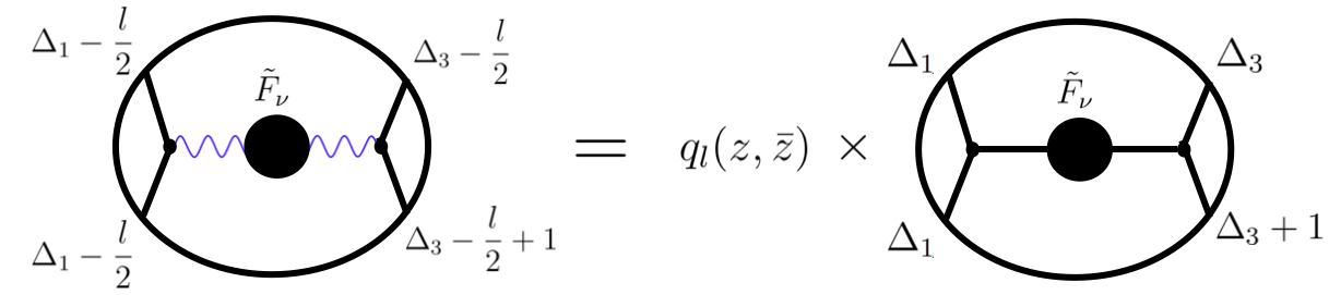
Figure 14: Showing the relation of Eq. 177 for the 4-point function, for $a=0$ and $b=\frac{1}{2}$ and $d=2$. The general ”blob” $\tilde{F}_{\nu}$ is the same on both sides.

C.2 A relation across dimensions $d$

Let us recall the expression for a ”Blob diagram” Eq. 22:

$$g^{(\Delta_{i})}_{l,d}(z,\bar{z})=\int d\nu\tilde{F}_{\nu,l}\times T_{\nu,l,d}^{(\Delta_{i})}\times\mathcal{K}^{\Delta_{i}}_{\frac{d}{2}+i\nu,l}(z,\bar{z})$$ (178)

where we defined

$$T_{\nu,l,d}^{(\Delta_{i})}\equiv\frac{\Upsilon_{\nu,l}^{\Delta_{i}}}{\sin\pi(\frac{\Delta_{1}+\Delta_{2}+l}{2}-\frac{d}{4}-\frac{i\nu}{2})\sin\pi(\frac{\Delta_{3}+\Delta_{4}+l}{2}-\frac{d}{4}-\frac{i\nu}{2})}$$ (179)

$\Delta_{i}$ are the external scaling dimensions. Recall that the conformal blocks in $d=2$ and $d=4$ are a symmetrized sum in $z$, $\bar{z}$:

$$\mathcal{K}^{\Delta_{i}}_{\Delta,l,d=2}(z,\bar{z})=\frac{1}{1+\delta_{l,0}}\Big{(}k_{\Delta-l}^{(a,b)}(z)k_{\Delta+l}^{(a,b)}(\bar{z})+k_{\Delta+l}^{(a,b)}(z)k_{\Delta-l}^{(a,b)}(\bar{z})\Big{)}$$

$$\mathcal{K}^{\Delta_{i}}_{\Delta,l,d=4}(z,\bar{z})=\frac{z\bar{z}}{z-\bar{z}}\Big{(}k_{\Delta-l-2}^{(a,b)}(z)k_{\Delta+l}^{(a,b)}(\bar{z})-k_{\Delta+l}^{(a,b)}(z)k_{\Delta-l-2}^{(a,b)}(\bar{z})\Big{)}$$ (180)

Thus we can write Eq. 178 as:

$$g^{(\Delta_{i})}_{l,d}(z,\bar{z})=\int_{-\infty}^{\infty}d\nu\ \widetilde{g}^{(\Delta_{i})}_{\nu,l,d}(z,\bar{z})+\int_{-\infty}^{\infty}d\nu\ \widetilde{g}^{(\Delta_{i})}_{\nu,l,d}(\bar{z},z)$$ (181)

where

$$\widetilde{g}^{(\Delta_{i})}_{\nu,l,d=2}(z,\bar{z})\equiv\frac{1}{1+\delta_{l,0}}\tilde{F}_{\nu,l}\times T_{\nu,l,d=2}^{(\Delta_{i})}\times k_{i\nu+1-l}^{(a,b)}(z)k_{i\nu+1+l}^{(a,b)}(\bar{z})$$ (182)

and

$$\widetilde{g}^{(\Delta_{i})}_{\nu,l,d=4}(z,\bar{z})\equiv\frac{z\bar{z}}{z-\bar{z}}\tilde{F}_{\nu,l}\times T_{\nu,l,d=4}^{(\Delta_{i})}\times k_{i\nu-l}^{(a,b)}(z)k_{i\nu+2+l}^{(a,b)}(\bar{z})$$ (183)

Now we will find a relation between $\widetilde{g}^{(\Delta_{i})}_{\nu,l,d=2}(z,\bar{z})$ and $\widetilde{g}^{(\Delta_{i})}_{\nu,l,d=4}(z,\bar{z})$, Eqs. 182 and 183. Consider the following transformation:

$$(l,d,\Delta_{i})\longrightarrow(l-1,d+2,\Delta_{i}+1)$$ (184)

This is a transformation that simultaneously changes the spin, the space-time dimension, and the scaling dimensions of a blob diagram. Under this transformation we have (Eq. 21 and 179):

$$T_{\nu,l-1,d=4}^{(\Delta_{i}+1)}=(1+\delta_{l,0})\frac{z\bar{z}}{z-\bar{z}}(i\nu)T_{\nu,l,d=2}^{(\Delta_{i})}$$ (185)

and thus we get the relation:

$$\boxed{\widetilde{g}_{\nu,l-1,d=4}^{(\Delta_{i}+1)}(z,\bar{z})=(1+\delta_{l,0})\frac{z\bar{z}}{z-\bar{z}}\times(i\nu)\widetilde{g}_{\nu,l,d=2}^{(\Delta_{i})}(z,\bar{z})}$$ (186)

This relation connects ”blob diagrams” in $d=2$ and $d=4$. In $d=6$ the conformal block is likewise a sum of product of functions $k_{\Delta}^{(a,b)}(z)$ Dolan:2011dv . We expect to have a relation connecting blob diagrams in $d=6$ and $d=2,4$.

References

- (1) H. Liu, “Scattering in anti-de Sitter space and operator product expansion,” Phys. Rev. D60 (1999) 106005, arXiv:hep-th/9811152 [hep-th].
- (2) H. Liu and A. A. Tseytlin, “On four point functions in the CFT / AdS correspondence,” Phys. Rev. D59 (1999) 086002, arXiv:hep-th/9807097 [hep-th].
- (3) F. A. Dolan and H. Osborn, “Conformal four point functions and the operator product expansion,” Nucl. Phys. B599 (2001) 459–496, arXiv:hep-th/0011040 [hep-th].
- (4) D. Z. Freedman, S. D. Mathur, A. Matusis, and L. Rastelli, “Correlation functions in the CFT(d) / AdS(d+1) correspondence,” Nucl. Phys. B546 (1999) 96–118, arXiv:hep-th/9804058 [hep-th].
- (5) E. D’Hoker and D. Z. Freedman, “General scalar exchange in AdS(d+1),” Nucl. Phys. B550 (1999) 261–288, arXiv:hep-th/9811257 [hep-th].
- (6) D. Z. Freedman, S. D. Mathur, A. Matusis, and L. Rastelli, “Comments on 4 point functions in the CFT / AdS correspondence,” Phys. Lett. B452 (1999) 61–68, arXiv:hep-th/9808006 [hep-th].
- (7) E. D’Hoker and D. Z. Freedman, “Gauge boson exchange in AdS(d+1),” Nucl. Phys. B544 (1999) 612–632, arXiv:hep-th/9809179 [hep-th].
- (8) E. D’Hoker, D. Z. Freedman, and L. Rastelli, “AdS / CFT four point functions: How to succeed at z integrals without really trying,” Nucl. Phys. B562 (1999) 395–411, arXiv:hep-th/9905049 [hep-th].
- (9) X. Zhou, “Recursion Relations in Witten Diagrams and Conformal Partial Waves,” JHEP 05 (2019) 006, arXiv:1812.01006 [hep-th].
- (10) S. Raju, “BCFW for Witten Diagrams,” Phys. Rev. Lett. 106 (2011) 091601, arXiv:1011.0780 [hep-th].
- (11) S. Raju, “Recursion Relations for AdS/CFT Correlators,” Phys. Rev. D83 (2011) 126002, arXiv:1102.4724 [hep-th].
- (12) S. Albayrak, C. Chowdhury, and S. Kharel, “New relation for AdS amplitudes,” arXiv:1904.10043 [hep-th].
- (13) S. Albayrak and S. Kharel, “Towards the higher point holographic momentum space amplitudes,” JHEP 02 (2019) 040, arXiv:1810.12459 [hep-th].
- (14) S. Albayrak, S. Kharel, and D. Meltzer, “On duality of color and kinematics in (A)dS momentum space,” JHEP 03 (2021) 249, arXiv:2012.10460 [hep-th].
- (15) S. Albayrak, C. Chowdhury, and S. Kharel, “Study of momentum space scalar amplitudes in AdS spacetime,” Phys. Rev. D 101 no. 12, (2020) 124043, arXiv:2001.06777 [hep-th].
- (16) J. Penedones, “Writing CFT correlation functions as AdS scattering amplitudes,” JHEP 03 (2011) 025, arXiv:1011.1485 [hep-th].
- (17) A. L. Fitzpatrick, J. Kaplan, J. Penedones, S. Raju, and B. C. van Rees, “A Natural Language for AdS/CFT Correlators,” JHEP 11 (2011) 095, arXiv:1107.1499 [hep-th].
- (18) M. F. Paulos, “Towards Feynman rules for Mellin amplitudes,” JHEP 10 (2011) 074, arXiv:1107.1504 [hep-th].
- (19) L. Rastelli and X. Zhou, “How to Succeed at Holographic Correlators Without Really Trying,” JHEP 04 (2018) 014, arXiv:1710.05923 [hep-th].
- (20) L. Rastelli and X. Zhou, “Mellin amplitudes for ,” Phys. Rev. Lett. 118 no. 9, (2017) 091602, arXiv:1608.06624 [hep-th].
- (21) C. Cardona, “Mellin-(Schwinger) representation of One-loop Witten diagrams in AdS,” arXiv:1708.06339 [hep-th].
- (22) E. Y. Yuan, “Loops in the Bulk,” arXiv:1710.01361 [hep-th].
- (23) E. Y. Yuan, “Simplicity in AdS Perturbative Dynamics,” arXiv:1801.07283 [hep-th].
- (24) D. Carmi, L. Di Pietro, and S. Komatsu, “A Study of Quantum Field Theories in AdS at Finite Coupling,” JHEP 01 (2019) 200, arXiv:1810.04185 [hep-th].
- (25) D. Carmi, “Loops in AdS: from the spectral representation to position space,” JHEP 06 (2020) 049, arXiv:1910.14340 [hep-th].
- (26) D. Carmi, “Loops in AdS: from the spectral representation to position space. Part II,” JHEP 07 (2021) 186, arXiv:2104.10500 [hep-th].
- (27) Ankur, D. Carmi, and L. Di Pietro, “Scalar QED in AdS,” JHEP 10 (2023) 089, arXiv:2306.05551 [hep-th].
- (28) O. Aharony, L. F. Alday, A. Bissi, and E. Perlmutter, “Loops in AdS from Conformal Field Theory,” JHEP 07 (2017) 036, arXiv:1612.03891 [hep-th].
- (29) J. Henriksson and T. Lukowski, “Perturbative Four-Point Functions from the Analytic Conformal Bootstrap,” JHEP 02 (2018) 123, arXiv:1710.06242 [hep-th].
- (30) L. F. Alday and A. Bissi, “Loop Corrections to Supergravity on ,” Phys. Rev. Lett. 119 no. 17, (2017) 171601, arXiv:1706.02388 [hep-th].
- (31) L. F. Alday, A. Bissi, and E. Perlmutter, “Holographic Reconstruction of AdS Exchanges from Crossing Symmetry,” JHEP 08 (2017) 147, arXiv:1705.02318 [hep-th].
- (32) D. Mazac and M. F. Paulos, “The Analytic Functional Bootstrap I: 1D CFTs and 2D S-Matrices,” arXiv:1803.10233 [hep-th].
- (33) D. Carmi, J. Penedones, J. A. Silva, and A. Zhiboedov, “Applications of dispersive sum rules: -expansion and holography,” arXiv:2009.13506 [hep-th].
- (34) S. Caron-Huot and A.-K. Trinh, “All Tree-Level Correlators in AdSS5 Supergravity: Hidden Ten-Dimensional Conformal Symmetry,” arXiv:1809.09173 [hep-th].
- (35) L. F. Alday and S. Caron-Huot, “Gravitational S-matrix from CFT dispersion relations,” arXiv:1711.02031 [hep-th].
- (36) F. Aprile, J. M. Drummond, P. Heslop, and H. Paul, “Quantum Gravity from Conformal Field Theory,” JHEP 01 (2018) 035, arXiv:1706.02822 [hep-th].
- (37) F. Aprile, J. M. Drummond, P. Heslop, and H. Paul, “Loop corrections for Kaluza-Klein AdS amplitudes,” JHEP 05 (2018) 056, arXiv:1711.03903 [hep-th].
- (38) A. Bissi, G. Fardelli, and A. Georgoudis, “All loop structures in Supergravity Amplitudes on from CFT,” arXiv:2010.12557 [hep-th].
- (39) A. Bissi, G. Fardelli, and A. Georgoudis, “Towards All Loop Supergravity Amplitudes on ,” arXiv:2002.04604 [hep-th].
- (40) A. L. Fitzpatrick, E. Katz, D. Poland, and D. Simmons-Duffin, “Effective Conformal Theory and the Flat-Space Limit of AdS,” JHEP 07 (2011) 023, arXiv:1007.2412 [hep-th].
- (41) A. L. Fitzpatrick and J. Kaplan, “Analyticity and the Holographic S-Matrix,” JHEP 10 (2012) 127, arXiv:1111.6972 [hep-th].
- (42) D. Ponomarev, “From bulk loops to boundary large-N expansion,” arXiv:1908.03974 [hep-th].
- (43) I. Bertan and I. Sachs, “Loops in Anti–de Sitter Space,” Phys. Rev. Lett. 121 no. 10, (2018) 101601, arXiv:1804.01880 [hep-th].
- (44) I. Bertan, I. Sachs, and E. D. Skvortsov, “Quantum Theory in AdS4 and its CFT Dual,” arXiv:1810.00907 [hep-th].
- (45) M. Beccaria and A. A. Tseytlin, “On boundary correlators in Liouville theory on AdS2,” JHEP 07 (2019) 008, arXiv:1904.12753 [hep-th].
- (46) A. L. Fitzpatrick and J. Kaplan, “Unitarity and the Holographic S-Matrix,” JHEP 10 (2012) 032, arXiv:1112.4845 [hep-th].
- (47) S. Giombi, C. Sleight, and M. Taronna, “Spinning AdS Loop Diagrams: Two Point Functions,” JHEP 06 (2018) 030, arXiv:1708.08404 [hep-th].
- (48) A. Costantino and S. Fichet, “Opacity from Loops in AdS,” JHEP 02 (2021) 089, arXiv:2011.06603 [hep-th].
- (49) A. Antunes, M. S. Costa, T. Hansen, A. Salgarkar, and S. Sarkar, “The perturbative CFT optical theorem and high-energy string scattering in AdS at one loop,” arXiv:2012.01515 [hep-th].
- (50) D. Meltzer, E. Perlmutter, and A. Sivaramakrishnan, “Unitarity Methods in AdS/CFT,” JHEP 03 (2020) 061, arXiv:1912.09521 [hep-th].
- (51) B. Nagaraj and D. Ponomarev, “Spinor-helicity formalism for massless fields in AdS4 III: contact four-point amplitudes,” JHEP 08 no. 08, (2020) 012, arXiv:2004.07989 [hep-th].
- (52) D. Meltzer and A. Sivaramakrishnan, “CFT unitarity and the AdS Cutkosky rules,” JHEP 11 (2020) 073, arXiv:2008.11730 [hep-th].
- (53) S. Albayrak and S. Kharel, “Spinning loop amplitudes in anti–de Sitter space,” Phys. Rev. D 103 no. 2, (2021) 026004, arXiv:2006.12540 [hep-th].
- (54) X. Zhou, “How to Succeed at Witten Diagram Recursions without Really Trying,” JHEP 08 (2020) 077, arXiv:2005.03031 [hep-th].
- (55) L. Eberhardt, S. Komatsu, and S. Mizera, “Scattering equations in AdS: scalar correlators in arbitrary dimensions,” JHEP 11 (2020) 158, arXiv:2007.06574 [hep-th].
- (56) M. S. Costa, V. Gonçalves, and J. Penedones, “Spinning AdS Propagators,” JHEP 09 (2014) 064, arXiv:1404.5625 [hep-th].
- (57) F. A. Dolan and H. Osborn, “Conformal Partial Waves: Further Mathematical Results,” arXiv:1108.6194 [hep-th].
- (58) R. D. Pisarski, “Chiral Symmetry Breaking in Three-Dimensional Electrodynamics,” Phys. Rev. D 29 (1984) 2423.
- (59) T. W. Appelquist, M. J. Bowick, D. Karabali, and L. C. R. Wijewardhana, “Spontaneous Chiral Symmetry Breaking in Three-Dimensional QED,” Phys. Rev. D 33 (1986) 3704.
- (60) T. Appelquist, D. Nash, and L. C. R. Wijewardhana, “Critical Behavior in (2+1)-Dimensional QED,” Phys. Rev. Lett. 60 (1988) 2575.
- (61) C. D. Roberts and A. G. Williams, “Dyson-Schwinger equations and their application to hadronic physics,” Prog. Part. Nucl. Phys. 33 (1994) 477–575, arXiv:hep-ph/9403224.
- (62) D. Carmi and S. Caron-Huot, “A Conformal Dispersion Relation: Correlations from Absorption,” JHEP 09 (2020) 009, arXiv:1910.12123 [hep-th].
- (63) D. Carmi, J. Moreno, and S. Sukholuski, “A CFT Dispersion relation for mixed correlators,”.
- (64) L. Di Pietro, V. Gorbenko, and S. Komatsu, “Cosmological Correlators at Finite Coupling,” arXiv:2312.17195 [hep-th].
- (65) J. Liu, E. Perlmutter, V. Rosenhaus, and D. Simmons-Duffin, “-dimensional SYK, AdS Loops, and Symbols,” arXiv:1808.00612 [hep-th].
- (66) S. Caron-Huot, “Analyticity in Spin in Conformal Theories,” JHEP 09 (2017) 078, arXiv:1703.00278 [hep-th].