Weisfeiler Leman for Euclidean Equivariant Machine Learning

Abstract

The $k$-Weifeiler-Leman ($k$-WL) graph isomorphism test hierarchy is a common method for assessing the expressive power of graph neural networks (GNNs). Recently, the $2$-WL test was proven to be complete on weighted graphs which encode $3\mathrm{D}$ point cloud data. Consequently, GNNs whose expressive power is equivalent to the $2$-WL test are provably universal on point clouds. Yet, this result is limited to invariant continuous functions on point clouds.

In this paper we extend this result in three ways: Firstly, we show that $2$-WL tests can be extended to point clouds which include both positions and velocity, a scenario often encountered in applications. Secondly, we show that PPGN (Maron et al., 2019a) can simulate $2$-WL uniformly on all point clouds with low complexity. Finally, we show that a simple modification of this invariant PPGN architecture can be used to obtain a universal equivariant architecture that can approximate all continuous equivariant functions uniformly.

Building on our results, we develop our WeLNet architecture, which can process position-velocity pairs, compute functions fully equivariant to permutations and rigid motions, and is provably complete and universal. Remarkably, WeLNet is provably complete precisely in the setting in which it is implemented in practice. Our theoretical results are complemented by experiments showing WeLNet sets new state-of-the-art results on the N-Body dynamics task and the GEOM-QM9 molecular conformation generation task.

1 Introduction

Machine learning (ML) models that are equivariant to group symmetries of data, have been at the focal point of recent research. Example range from CNNs that respect the translation symmetry of images, through graph neural networks (GNNs) that enforce permutation invariance to account for the invariance of the order of a node’s neighbors, to models which respect symmetries of the Lornentz (Bogatskiy et al., 2020) or special linear group (Lawrence & Harris, 2023).

In this paper our focus will be on equivariant models for point clouds. A point cloud is a finite collection of points, usually in $\mathbb{R}^{3}$, with the natural symmetry of invariance to permutation. Point clouds are flexible objects which are used to represent discretized surfaces , molecules and particles (Cvrtila & Rot, 2022). In many of these setting, point clouds have an additional natural symmetry to rotations and translation. Due to their applications in chemoinformatics (Pozdnyakov & Ceriotti, 2023), particle dynamics (Schütt et al., 2017), and computer vision (Qi et al., 2017), point cloud networks with permutation, rotation and translation symmetries have attracted a lot of attention in recent years (Thomas et al., 2018; Victor Garcia Satorras, 2021; Deng et al., 2021; Du et al., 2022).

One interesting paradigm for creating equivariant networks for point clouds goes through the observation that point clouds are determined, up to group symmetries, by their pairwise distance matrix. Each such matrix can be identified with a complete weighted graph. Using this identification, point-cloud neural networks can be constructed by applying standard GNNs to the point cloud’s distance matrix (Lim et al., 2022).

Several recent works have attempted to address the theoretical potential and limitations of these graph-based equivariant models. The primary approach is via $k$-WL tests (Weisfeiler & Leman, 1968), a hierarchy of tests which is the predominant method for assessing the expressive power of GNNs on combinatorial graphs (Morris et al., 2020). For GNNs applied to point clouds, (Pozdnyakov & Ceriotti, 2022) showed that there exist pairs of non-equivalent point clouds which cannot be distinguished by any GNN whose expressive power is bounded by $1$-WL. This suggests that the capacity of such GNNs, which include the popular Message Passing GNNs (Xu et al., 2018), is limited, and more expressive GNNs may be needed for some geometric tasks.

In a recent breakthrough, Hordan et al.; Rose et al. have shown that the 2-WL graph isomorphism test for point clouds is complete: that is, $2$-WL can distinguish between all non-equivalent 3D point clouds. As a corollary, it can be shown that GNNs that can simulate the $2$-WL test, combined with suitable pooling operators, can approximate all continuous functions invariant to permutations, rotations and translations (Hordan et al., 2023; Li et al., 2023). These theoretical findings are coupled with strong empirical results attained by Li et al. with $2$-WL-based methods for invariant tasks.

It may be argued that these recent results indicate that $2$-WL based methods are well suited for learning on point clouds, particularly for small molecules and dynamical systems, where low data dimensionality makes $2$-WL like methods computationally feasible. Furthermore, these methods can overcome the inherent limitations of models bounded by $1$-WL on molecular tasks and on other datasets with a high degree of data symmetry (Pozdnyakov et al., 2020; Li et al., 2023). Nonetheless, 2-WL-based methods are less studied than other research directions in the equivariant point cloud literature, and several practical and theoretical challenges remain. In this paper we address three such important challenges:

Firstly, the input to point-cloud tasks that originate from physical simulation is often not one, but two points clouds: one defining particle positions, the other defining particle velocity. It is a desideratum to construct an architecture that is complete with respect to such data, that is, it can distinguish among all position-velocity pairs up to symmetries.

Secondly, the universality results stated above assume an implementation of GNNs that can simulate the $2$-WL test. While the PPGN (Maron et al., 2019a) architecture is indeed known to simulate the $2$-WL test, it is only guaranteed to separate different graph pairs using different network parameters. To date, it is not clear that $2$-WL can be simulated by a network with fixed parameters uniformly on all point clouds of size $n$. Moreover, even for pairwise separation, the time complexity in the proof in (Maron et al., 2019a) is prohibitively high: the time complexity of a PPGN block is estimated at $\mathcal{O}{(N_{F}\cdot n^{\omega})}$, where $n^{\omega}$ is the complexity of matrix multiplication and $N_{F}$ denotes the dimension of the edge features. In the proof in (Maron et al., 2019a), this dimension grows exponentially both in the number of iterations and in the number of input features.

Lastly, existing universality results for $2$-WL-based methods for point clouds are restricted to permutation- and rotation- invariant functions, or to functions that are permutation invariant and rotation equivariant. The case of functions that are jointly permutation- and rotation-equivariant is more difficult to analyze, and has not been addressed to date, despite its relevance for particle dynamics.

1.1 Contributions

The three contributions of this manuscript address these three challenges:

Contribution 1: Combining positions and velocities We suggest an adaptation of the $2$-WL test to the case of position-velocity pairs, and show this test is complete. These results can also be easily extended to cases where additional geometric node features such as forces, or non-geometric features such as atomic numbers, are present.

Contribution 2: Cardinality of $2$-WL simulation We show that PPGN with a fixed finite number of parameters can uniformly separate continuous families of $2$-WL separable graphs, and in particular all $3\mathrm{D}$ point clouds. The number of parameters depends moderately on the intrinsic dimension of these continuous graph families. Consequently, the memory and runtime complexity reduces to $\mathcal{O}(n^{2})$ and $\mathcal{O}(n^{\omega})$, respectively. This result particularly applies to weighted graphs derived from point clouds, but it is also of independent interest for general graphs processed by the most studied general $k$-WL based GNNs (Maron et al., 2019a; Morris et al., 2018), as we prove separation for a general family of weighted graphs.

Contribution 3: Equivariant Universality We propose a simple method to obtain an equivariant architecture from the invariant $2$-WL based PPGN architecture and show that this architecture is universal. That is, it can approximate all continuous equivariant functions, uniformly on compact sets.

Building on these results, we introduce our Weisfeiler-Leman Network architecture, WeLNet , which can process position-velocity pairs, produce functions fully equivariant to permutations, rotations, and translation, and is provably complete and universal.

A unique property of WeLNet is that for Lebesgue almost every choice of its parameters, it is provably complete precisely in the settings in which it is implemented in practice. This is in contrast with previous complete constructions, which typically require an unrealistically large number of parameters to be provably complete, such as ClofNet (Du et al., 2022), GemNet (Gasteiger et al., 2021) and TFN(Thomas et al., 2018; Dym & Maron, 2020).

Our experiments show that WeLNet compares favorably with state of the art architectures for the $\mathrm{N}$-body physical simulation tasks and molecular conformation generation. Additionally, we empirically validate our theory by showing that PPGN can separate challenging pairs of $2$-WL separable graphs with a very small number of features per edge. This effect is especially pronounced for analytic non-polynomial activations, where a single feature per edge is provably sufficient.

2 Problem Setup

2.1 Mathematical Notation

A (finite) multiset $\{\!\!\{y_{1},\ldots,y_{N}\}\!\!\}$ is an unordered collection of elements where repetitions are allowed.

Let $\mathcal{G}$ be a group acting on a set $\mathcal{X}$. For $X,Y\in\mathcal{X}$, we say that $X\cong Y$ if $Y=gX$ for some $g\in\mathcal{G}$. We say that a function $f:\mathcal{X}\to\mathcal{Y}$ is invariant if $f(gx)=f(x)$ for all $x\in X,g\in G$. We say that $f$ is equivariant if $\mathcal{Y}$ is also endowed with some action of $G$ and $f(gx)=gf(x)$ for all $x\in\mathcal{X},g\in\mathcal{G}$.

In this paper, we consider the set $\mathcal{X}=\mathbb{R}^{6\times n}$ and regard it as a set of pairs $(X,V)$, with $X,V\in\mathbb{R}^{3\times n}$ denoting the positions and velocities of $n$ particles in $\mathbb{R}^{3}$. We denote the $n$ columns of $X$ and $V$ by $x_{i}$ and $v_{i}$ respectively, $i=1,\ldots,n$. The natural symmetries of $(X,V)$ are permutations, rotations, and translations. Formally, we say that $(X,V)\cong(X^{\prime},V^{\prime})$ if there exist a permutation $\tau$, a (proper or improper) rotation $R\in O(3)$, and a ‘translation’ vector $t$, such that

$$(x_{1}^{\prime},\ldots,x_{n}^{\prime}) =(Rx_{\tau(1)}+t,\ldots,Rx_{\tau(n)}+t)$$

$$(v_{1}^{\prime},\ldots,v_{n}^{\prime}) =(Rv_{\tau(1)},\ldots,Rv_{\tau(n)})$$

We consider functions $f:\mathbb{R}^{6\times n}\to\mathbb{R}^{6\times n}$ (and scalar functions $f:\mathbb{R}^{6\times n}\to\mathbb{R}$) that are equivariant (respectively invariant) to permutations, rotations, and translations.

Description of additional related works, and proofs of all theorem, are given in the appendix.

2.2 2-WL Tests

The $2$-WL test is a test for determining whether a given pair of graphs are isomorphic (that is, related by a permutation). It is defined as follows: let $\mathcal{G}$ be a graph with vertices indexed by $[n]=\{1,2,\ldots,n\}$, possibly endowed with node features $w_{v}$ and edge features $w_{u,v}$. We denote each ordered pair of vertices by a multi-index $\mathbf{i}=\left(i_{1},i_{2}\right)\in[n]^{2}$. For each such pair $\mathbf{i}$, the $2$-WL test maintains a coloring $\mathbf{C}(\mathbf{i})$ that belongs to a discrete set, and updates it iteratively. First, the coloring of each pair $\mathbf{i}$ is assigned an initial value $\mathbf{C_{(0)}}(\mathbf{i})$ that encodes whether there is an edge between the paired nodes $i_{1}$ and $i_{2}$, and the value of that edge’s feature $w_{i_{1},i_{2}}$, if given as input. Node features $w_{i}$ are encoded in this initial coloring through pairs of identical indices $\mathbf{i}=(i,i)$. Then the color of each pair $\mathbf{i}$ is iteratively updated according to the colors of its ‘neighboring’ pairs. The colors of neighboring pairs is aggregated to an ‘intermediate color’ $\mathbf{\tilde{C}_{(t+1)}}(\mathbf{i})$,

$$\mathbf{\tilde{C}_{(t+1)}}(\mathbf{i})=\text{{HASH}}(\{\!\!\{\mathbf{C_{(\mathbf{t})}}(i_{1},j),C_{(\mathbf{t})}(j,i_{2})\}\!\!\}_{j=1}^{n})$$ (1)

This ‘intermediate color’ is then combined with the previous color at $\mathbf{i}$ to form the new color

$$\mathbf{C_{(t+1)}}(\mathbf{i})=\text{{HASH}}\left(\mathbf{{C}_{(t)}}(\mathbf{i}),\mathbf{\tilde{C}_{(t+1)}}(\mathbf{i})\right)$$ (2)

This process is repeated $T$ times to obtain a final coloring $\{\!\!\{\mathbf{C_{(T)}}(\mathbf{i})\}\!\!\}_{\mathbf{i}\in{\left[n\right]^{2}}}$. A global label is then calculated by

$$\mathbf{C}_{\mathrm{global}}=\text{{HASH}}\left(\{\!\!\{\mathbf{C_{(T)}}(\mathbf{i})\;|\;\mathbf{i}\in[n]^{2}\}\!\!\}\right).$$ (3)

To check isomorphism of two graphs $G,G^{\prime}$, this process is run simultaneously for both graphs to produce global features $\mathbf{C}_{\mathrm{global}}$ and $\mathbf{C}_{\mathrm{global}}^{\prime}$. The HASH function is defined recursively throughout this process so that each new input encountered gets a distinct feature. If $G$ and $G^{\prime}$ are isomorphic, then by the permutation invariant nature of the test, $\mathbf{C}_{\mathrm{global}}=\mathbf{C}_{\mathrm{global}}^{\prime}$. Otherwise, for ‘nicely behaved’ non-isomorphic graphs the final global features will be distinct, but there are pathological graph pairs for which identical features will be obtained. Thus, the $2$-WL test is not complete on the class of general graphs.

2.3 Geometric 2-WL Tests

We now turn to the geometric setting. Here we are given two point clouds $X,X^{\prime}\in\mathbb{R}^{3\times n}$ (we will discuss including velocities later), and our goal is to devise a test to check whether they are equivalent up to permutation, rotation, and translation. As observed in e.g, (Victor Garcia Satorras, 2021), this problem can be equivalently rephrased as the problem of distinguishing between two (complete) weighted graphs $\mathcal{G}(X)$ and $\mathcal{G}(X^{\prime})$ whose nodes correspond to the indices of the points, and whose edge weights encode the pairwise distances $\|x_{i}-x_{j}\|$ (respectively, $\|x_{i}^{\prime}-x_{j}^{\prime}\|$). The two weighted graphs $\mathcal{G}(X)$ and $\mathcal{G}(X^{\prime})$ are isomorphic (that is, related by a permutation) if and only if $X\cong X^{\prime}$. Accordingly, we obtain a test to check whether $X\cong X^{\prime}$ by applying the $2$-WL test to the corresponding graphs $\mathcal{G}(X)$ and $\mathcal{G}(X^{\prime})$ and checking whether they yield an identical output. As mentioned earlier, Rose et al. showed that in the 3D geometric setting, the 2-WL test is complete. That is, the $2$-WL test will assign the same global feature to $\mathcal{G}(X)$ and $\mathcal{G}(X^{\prime})$ if, and only if, the point clouds $X,X^{\prime}$ are related by permutation, rotation, and translation.

Note that, although the $2$-WL test is typically applied to pairs of ‘discrete’ graphs, it can easily be applied to a pair of graphs with ‘continuous features’, since ultimately for a fixed pair of graphs the number of features is finite. The main challenge in the continuous feature case is replacing the HASH functions with functions which are both differentiable, and are injective on an (uncountably) infinite, continuous, feature space. These issues are addressed in our second contribution on simulating $2$-WL tests with differentiable models (Section 4).

In the three following sections we will address the three challenges outlined in Section 1.1. In Section 3 we discuss how to define 2-WL tests that are complete when applied to position-velocity pairs $(X,V)$. In Section 4 we show that the PPGN architecture can simulate 2-WL tests, even with a continuum of features, with relatively low complexity. In Section 5 we show that the PPGN architecture, combined with an appropriate pooling operation, is a universal approximator of continuous functions that are equivariant to permutations, rotations and translations.

2.4 Extensions and Limitations

There are many variants of the setting above which could be considered: $O(d)$ equivariance with $d\neq 3$, allowing only proper rotations in $SO(d)$ rather than all rotations, and allowing multiple equivariant features per node rather than just a position-velocity pair. In Appendix A we outline how our approach can be extended to these scenarios.

Our universality results hold only for complete distance matrices and not graphs with a notion of a local neighborhood. Often in applications, a distance threshold is used to allow for better complexity, The theoretical results presented in this manuscript cannot be directly applied to this setting, though the WeLNet architecture can be adapted to these cases easily.

3 $2$-WL for Position-Velocity Pairs

In this section we describe our first contribution. We consider the setting of particle dynamics tasks, in which the input is not only the particle positions $X$ but also the velocities $V$. In this setting, we define a weighted graph $\mathcal{G}(X,V)$ and prove that the $2$-WL test applied to such graphs is complete.

The edge weights $w_{i,j}$ of the weighted graph $\mathcal{G}(X,V)$ will consist of the $4\times 4$ pairwise distance matrix of the vectors $x_{i},x_{j},v_{i},v_{j}$ after centralizing $X$, that is

$$w_{i,j}=\mathrm{dist}\left(x_{i}-\frac{1}{n}\sum_{k=1}^{n}x_{k},x_{j}-\frac{1}{n}\sum_{k=1}^{n}x_{k},v_{i},v_{j}\right).$$ (4)

Note that this edge feature is invariant to rotation and translation. Additionally, since translation does not affect velocity, we add the norms of the velocity vectors $v_{i}$ as node features $w_{i}=\|v_{i}\|$.

We prove that the $2$-WL test applied to $\mathcal{G}(X,V)$ with the node and edge features induced from $(X,V)$, is complete with respect to the action of permutation, rotation and translation defined in Subsection 2.1:

Theorem 3.1.

Let $X,V,X^{\prime},V^{\prime}\in\mathbb{R}^{3\times n}$. Let $\mathbf{c}_{\mathrm{global}}$ and $\mathbf{c}_{\mathrm{global}}^{\prime}$ be the global features obtained from applying three iterations of the $2$-WL test to $\mathcal{G}(X,V)$ and $\mathcal{G}(X^{\prime},V^{\prime})$, respectively. Then

$$\mathbf{c}_{\mathrm{global}}=\mathbf{c}_{\mathrm{global}}^{\prime}\text{ if and only if }(X,V)\cong(X^{\prime},V^{\prime}).$$

Proof Sketch. The proof is based on a careful adaptation of the completeness proof in (Rose et al., 2023). The original proof, which only considered position inputs $X\in\mathbb{R}^{3\times n}$, reconstructs $X$ from its $2$-WL coloring, up to equivalence, in a two-step process: first, three ‘good’ (centralized) points $x_{i},x_{j},x_{k}$ are reconstructed, and then the rest of $X$ is reconstructed from the coloring of the pairs containing these three points. In our proof we show that a similar argument can be made in the $(X,V)$ setting, where now the three ‘good’ points could be either velocity or (centralized) position vectors, e.g. $x_{i},x_{j},v_{k}$, and they can be used to reconstruct both $X$ and $V$, up to equivalence. ∎

4 Simulation of $2$-WL with Exponentially Lower Complexity

In this section we discuss our second contribution regarding designing neural networks which simulate the $2$-WL test.

Models that simulate the $2$-WL test replace the HASH functions the test used, which are defined anew for every graph pair, with differentiable functions which are globally defined on all graphs.

The three main models proposed in the literature for simulating $2$-WL (equivalently, the $3$-OWL test, see (Morris et al., 2021)) are the $3$-GNN model from (Morris et al., 2018), and the $3$-EGN and PPGN models from (Maron et al., 2019a). Following Li et al., we focus on PPGN in our analysis and implementation, as this model is more efficient than the rest due to an elegant usage of matrix multiplications.

We start by describing the PPGN model. Then we explain in what sense existing results have shown that it simulates the $2$-WL test, and explain the shortcomings of these previous results. We then provide new, significantly stronger separation results . We note that this section is relevant for any choice of continuous or discrete labeling used to initialize $2$-WL, and thus should be of interest to graph neural network research also beyond the scope of its applications to Euclidean point clouds.

4.1 PPGN architecture

The input to the PPGN architecture is the same as to the $2$-WL test, that is, the same collection of pairwise features

$$\mathbf{c}_{(0)}(\mathbf{i})=\mathbf{C}_{(0)}(\mathbf{i})\text{ where }\mathbf{i}=(i_{1},i_{2})\in[n]^{2}$$ (5)

obtained from the input graph $\mathcal{G}$. We will assume that all graphs have $n$ vertices and their edge and node features are $D$ dimensional. We denote the collection of all such graphs by $\mathbb{G}_{n,D}$,

Similarly to $2$-WL, PPGN iteratively defines new pairwise features $\mathbf{c}_{(t+1)}$ from the previous features $\mathbf{c}_{(t)}$ using an aggregation and combination step, the only difference being that now the HASH functions are replaced by differentiable functions. Specifically, the aggregation function used by PPGN involves two MLPs $\phi^{(1,t)}$ and $\phi^{(2,t)}$:

$$\tilde{\mathbf{c}}_{(t+1)}(\mathbf{i})=\sum_{j=1}^{n}\phi^{(1,t)}\left(\mathbf{c}_{(t)}(i_{1},j)\right)\odot\phi^{(2,t)}\left(\mathbf{c}_{(t)}(j,i_{2})\right).$$ (6)

Here the output of the two MLPs has the same dimension, which we denote by $D_{(t+1)}$, and $\odot$ denotes the entrywise (Hadamard) product. Note that (6) can be implemented by independently computing $D_{(t+1)}$ matrix products.

We note that (6), which corresponds to (1) in the combinatorial case, is a well-defined function on the multiset $\{\!\!\{(\mathbf{c_{(\mathbf{t})}}(i_{1},j),\mathbf{c}_{(\mathbf{t})}(j,i_{2})\}\!\!\}_{j=1}^{n}$; that is, permuting the $j$ index will not affect the result.

The combination step in PPGN involves a third MLP $\phi^{(3,t)}$, whose output dimension is also $D_{(t+1)}$:

$$\mathbf{c}_{(t+1)}(\mathbf{i})=\tilde{\mathbf{c}}_{(t+1)}(\mathbf{i})\odot\phi^{(3,t)}\left(\mathbf{c}_{(t)}(\mathbf{i})\right).$$ (7)

We note that in this choice of the combination step, we follow Li et al.. This product-based step is more computationally efficient than the original concatenation-based combination step of Maron et al.. We address the simpler concatenation-based combination step in Appendix A.

After $T$ iterations, a graph-level representation $\mathbf{c}_{\mathrm{global}}$ is computed via a ‘readout’ function that operates on the multiset of all $T$-level features $\{\!\!\{\mathbf{c}_{(T)}(\mathbf{i})\}\!\!\}_{\mathbf{i}\in[n]^{2}}$. This is done using a final MLP, denoted $\phi_{\text{READOUT}}$, via

$$\mathbf{c}_{\mathrm{global}}=\sum_{\mathbf{i}\in[n]^{2}}\phi_{\text{READOUT}}(\mathbf{c}_{(T)}(\mathbf{i})).$$

Analytic PPGN

The PPGN architecture implicitly depends on several components. In our analysis in the next subsection we will focus on a simple instantiation, where all intermediate dimensions are equal to the same number $\Delta$, that is $D_{(t)}=\Delta$ for $t=0,\ldots,T-1$, and the MLPs $\phi^{(s,t)}$, $s=1,2,3$ and $\phi_{\text{READOUT}}$ are shallow networks of the form $\rho(Ax+b)$, with $A\in\mathbb{R}^{\Delta\times\Delta}$, $b\in\mathbb{R}^{\Delta}$, and $\rho:\mathbb{R}\to\mathbb{R}$ being an analytic non-polynomial function applied element-wise. This includes common activations, such as tanh, silu, sigmoid and most other smooth activation functions, but does not include piecewise-linear activations such as ReLU and leaky ReLU (for more on this see Figure 1). Under these assumptions, a PPGN network is completely determined by the number of nodes $n$, input feature dimension $D$, hidden feature dimension $\Delta$, the number of iterations $T$, and the parameters of all the linear layers in the MLPs $\phi^{(s,t)}$ and $\phi_{\text{READOUT}}$, which we denote by $\theta$. We call a PPGN network satisfying all these assumption an analytic PPGN network, and denote it by $\mathrm{PPGN}_{\mathrm{an}}(\theta;\Delta,T)$.

4.2 PPGN separation

In (Maron et al., 2019a) it is proven that PPGN simulates $2$-WL in the following sense: firstly, by construction, if $\mathcal{G}$ and $\mathcal{G}^{\prime}$ cannot be separated by $2$-WL, then they cannot be separated by PPGN either. Conversely, if $\mathcal{G}$ and $\mathcal{G}^{\prime}$ represent graphs that are separated by $2$-WL, then PPGN with sufficiently large MLPs $\boldsymbol{\phi}$ will separate $\mathcal{G}$ and $\mathcal{G}^{\prime}$.

This result has two limitations. The first is that the size of the PPGN networks in the separation proof provided in (Maron et al., 2019a) is extremely large. Their construction relies on a power-sum polynomial construction whose cardinality depends exponentially on the input and number of 2-WL iterations $T$, coupled with an approximation of the polynomials by MLP — which leads to an even higher complexity. The second limitation is that the separation results obtained in (Maron et al., 2019a) are not uniform, but apply only to pairs of graphs. While this can be easily extended to uniform separation on all pairs of $2$-WL separable graphs coming from a finite family (see (Chen et al., 2019)), this is not the case for infinite families of graphs. Indeed, in our geometric setting, we would like to find a PPGN network of finite size and fixed parameters, that can separate all weighted graphs generated by $(X,V)$ pairs. This is an infinite, $6n$-dimensional family of weighted graphs.

In this paper we resolve both of these limitations. We first show that the cardinality required for pairwise separation is actually extremely small: analytic PPGN require only one-dimensional features for pairwise separation.

Theorem 4.1.

[2-WL pairwise separation] Let $(n,D,T)\in\mathbb{N}^{3}$ and set $\Delta=1$. Let $\mathcal{G},\mathcal{G}^{\prime}\in\mathbb{G}_{n,D}$ represent two graphs separable by $T$ iterations of $2$-WL. Then for Lebesgue almost every choice of the parameters $\theta$, the features $\mathbf{c}_{\mathrm{global}}$ and $\mathbf{c}_{\mathrm{global}}^{\prime}$ obtained from applying $\mathrm{PPGN}_{\mathrm{an}}(\theta;\Delta,T)$ to $\mathcal{G}$ and $\mathcal{G}^{\prime}$, repsectively, satisfy that $\mathbf{c}_{\mathrm{global}}\neq\mathbf{c}_{\mathrm{global}}^{\prime}$.

Next, we consider the issue of uniform separation. We assume that we are given a continuous family of graphs $\mathcal{X}$ in $\mathbb{G}_{n,D}$. Equivalently, by identifying graphs with the pairwise features derived from them, we can think of this as a family of tensors in $\mathbb{R}^{n\times n\times D}$. The size of MLPs we require in this case to guarantee uniform separation on all graphs in $\mathcal{X}$ will be $2\dim(\mathcal{X})+1$. In particular, if $\mathcal{X}$ is the collection of weighted graphs that represent distance matrices of $n$ points in $\mathbb{R}^{3}$, then $\mathcal{X}$ is of dimension $\dim(\mathbb{R}^{3\times n})=3n$ and we will require PPGN networks with features of dimension $D_{(t)}=6n+1$ for separation. If we consider all position-velocity pairs $X,V$, then the dimension of $\mathcal{X}$ will be $6n$, and thus the dimension required for separation will be $12n+1$. Finally, under the common assumption that in problems of interest, the domain $\mathcal{X}$ is some manifold of low intrinsic dimension $d$, then the feature dimension required for uniform separation on $\mathcal{X}$ will be just $2d+1$. The full statement of our theorem for uniform separation is:

Theorem 4.2.

[uniform 2-WL separation] Let $(n,D,T)\in\mathbb{N}^{3}$. Let $\mathcal{X}\subseteq\mathbb{G}_{n,D}$ be a $\sigma$-subanalytic set of dimension $d$ and set $\Delta=2d+1$. Then for Lebesgue almost every $\theta$ we have that $\mathcal{G},\mathcal{G}^{\prime}\in\mathcal{X}$ can be separated by $T$ iterations of 2-WL if and only if $\mathbf{c}_{\mathrm{global}}\neq\mathbf{c}_{\mathrm{global}}^{\prime}$, where $\mathbf{c}_{\mathrm{global}}$ and $\mathbf{c}_{\mathrm{global}}^{\prime}$ are obtained by applying $\mathrm{PPGN}_{\mathrm{an}}(\theta;\Delta,T)$ to $\mathcal{G}$ and $\mathcal{G}^{\prime}$, respectively.

In this theorem, we identify graphs $\mathcal{G}\in\mathcal{X}$ with the $n\times n\times D$ adjacency tensors describing them. A full formal definition of a $\sigma$-subanalytic set of $\mathbb{R}^{n\times n\times D}$ is beyond the scope of this paper, and can be found in (Amir et al., 2023). For our purposes, we note that this is a rather large class of sets, which includes sets defined by analytic and polynomial constraints, and their countable unions, as well as images of such sets under polynomial, semi-algebraic, and analytic functions. In particular Euclidean spaces like $\mathbb{R}^{6\times n}$ are $\sigma$-subanalytic and their image under semi-algebraic maps, such as the map that takes $(X,V)$ to the graph $\mathcal{G}(X,V)$ weighted by its distances, will also be a $\sigma$-subanalytic set of dimension $\leq 6n$.

Proof idea for Theorem 4.1 and Theorem 4.2 .

The proof of pairwise separation uses three steps. First, we show that at every layer, pairwise separation can be achieved via aggregations of the form of Equation 6 with arbitrarily wide neural networks $\phi^{(1,t)},\phi^{(2,t)}$, using density arguments. Next, since wide networks are linear combinations of shallow networks, it follows that there exists scalar networks $\phi^{(1,t)},\phi^{(2,t)}$ which achieves pairwise separation at every layer. Lastly, the analyticity of the network implies that this separation is in fact achieved almost everywhere at every layer, which then implies that pairwise separation can be achieved with almost all parameters across all layers simultaneously.

For uniform separation, we use the finite witness theorem from (Amir et al., 2023) that essentially claims that pairwise separating analytic functions can be extended to uniformly separating functions by taking $2d+1$ copies of the functions (with independently selected parameters). The independence of the dimension throughout the construction on the depth $T$ of the PPGN network is obtained using ideas from (Hordan et al., 2023). ∎

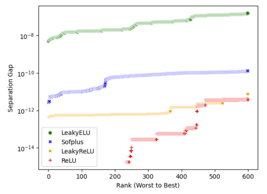
Figure 1: Separation results for PPGN on the EXP dataset with a single neuron per node. As our theorem predicts, the Sofplus and leaky ELU activations which are analtyic can separate all graph pairs with a single neuron per node. Non-analytic ReLU and leaky ReLU activations yield consistently diminished separation in comparison with their analytic counterparts.

4.3 Complexity

The complexity of PPGN is dependent on the output dimension of each update step and the complexity of matrix multiplication. Theorem 4.2 requires an output dimension which is only linearly dependent on the intrinsic dimension of size $d\ll n$, thus the computational complexity is that of matrix multiplication, that is $\mathcal{O}(n^{\omega})$, where, with naive implementation, $\omega=3$. Yet GPUs are especially adept at efficiently performing matrix multiplication, and, using the Strassen algorithm, this exponent can be reduced to $\omega=2.81$ (Cenk & Hasan, 2017).

4.4 Empirical Evaluation

We empirically evaluate our claims via a separation experiment on combinatorial graphs that are $2$-WL distinguishable, yet are $1$-WL indistinguishable, via the EXP (Abboud et al., 2020) dataset. It contains 600 $1$-WL equivalent graphs that can be distinguished by $2$-WL. We evaluate the separation power of PPGN models with a random initialization and a single neuron per edge on this dataset, as a function of the activation used. We ran the experiment with four different activations: the piecewise linear ReLU and LeakyReLU activations, and two roughly corresponding analytic activations: softplus and LeakyELU.

The results of the experiment are depicted in Figure 1, which shows the difference in the global features computed by PPGN for each of the 600 graph pairs and four activation types. The results show that the two analytic activations (as well as leakyReLU) succeeded in separating all graph pairs as predicted by our theory, but ReLU activations did not separate all graphs. We do find that with 15 features per edge ReLU too is able to attain perfect separation. We also note that the two analytic activations attained better separation gaps than the corresponding non-analytic activations. Finally, we note that in some cases, the separation attained is rather minor, with the difference between global features being as low as $10^{-12}$ .

5 Equivariant Universality on Point Clouds

In this section we discuss our third and final contribution, which is the construction of invariant and equivariant models for position-velocity pairs.

We note that the completeness of the $2$-WL test for position-velocity pairs, combined with our ability to simulate $2$-WL tests uniformly with analytic PPGNs, immediately implies that invariant models obtained by a composition of MLPs with the global feature $\mathbf{c}_{\mathrm{global}}=\mathbf{c}_{\mathrm{global}}(X,V)$ obtained from applying $\mathrm{PPGN}$ to $\mathcal{G}(X,V)$ are universal. That is, $\mathrm{MLP}\circ\mathbf{c}_{\mathrm{global}}(X,V)$, can approximate all continuous invariant functions. Similar universality results can be obtained for the permutation invariant and rotation equivariant case (Hordan et al., 2023).

Our goal is to address the more challenging case of universality for permutation, rotation and translation equivariant functions $f:\mathbb{R}^{6\times n}\to\mathbb{R}^{6\times n}$ rather than invariant functions. To achieve equivariant universality, we will define a simple pooling mechanism that enables obtaining node-level rotation, translation and permutation equivariant features $X^{\mathrm{out}}$ and rotation and permutation equivariant and translation invariant $V^{\mathrm{out}}$ from the rotation and translation invariant features of PPGN, and the input $(X,V)$. This step involves six MLPs $\psi_{(1)},\ldots,\psi_{(6)}$ and is defined as

$$x_{i}^{\mathrm{out}}=x_{i} +\psi_{(1)}(\mathbf{c}_{(T)}(i,i))v_{i}$$ (8)

$$+\sum_{k}\psi_{(2)}(\mathbf{c}_{(T)}(i,k))(x_{k}-x_{i})$$

$$+\sum_{k\neq i}\psi_{(3)}(\mathbf{c}_{(T)}(i,k))v_{k}$$

$$v_{i}^{\mathrm{out}}= \psi_{(4)}(\mathbf{c}_{(5)}(i,i))v_{i}$$ (9)

$$+\sum_{k}\psi_{(5)}(\mathbf{c}_{(T)}(i,k))(x_{k}-x_{i})$$

$$+\sum_{k\neq i}\psi_{(6)}(\mathbf{c}_{(T)}(i,k))v_{k}$$

The main result of this section is that the equivariant pooling layer defined above yields a universal equivariant architecture for position-velocity pairs $(X,V)$.

Theorem 5.1.

Let $\epsilon>0$. Let $\Psi:\mathbb{R}^{6\times n}\to\mathbb{R}^{6\times n}$ be a continuous permutation, rotation, and translation equivariant function. Denote $(X^{\mathrm{out}},V^{\mathrm{out}})=\Psi(X,V)$. Then $\Psi$ can be approximated to $\epsilon$ accuracy on compact sets in $\mathbb{R}^{6\times n}$ via the composition of the equivariant pooling layers defined in (8) and (9) with the features $\mathbf{c}_{(T)}(i,k)$ obtained from $\mathrm{PPGN}_{\mathrm{an}}(\theta;\Delta,T)$ iterations applied to $\mathcal{G}(X,V)$, with $T=5,\Delta=12n+1$ and appropriate parameters $\theta$.

Proof overview.

This proof consists of two main steps which we believe are of independent interest. The first step provides a characterization of polynomial functions $f:\mathbb{R}^{6\times n}\to\mathbb{R}^{6\times n}$ which are permutation, rotation and translation equivariant, in terms of expressions as in (8)-(9), but where the functions $\psi_{(j)}\circ\mathbf{c}_{(T)}(i,k)$ are replaced by polynomials $p_{i,k}$ with the same equivariant structure. This result gives a more explicit characterization of equivariant polynomials than the one in (Villar et al., 2021), and includes velocities and not only positions.

The second step of the proof shows that the $p_{i,k}$ polynomials can be approximated by the $\psi_{(j)}\circ\mathbf{c}_{(T)}(i,k)$ functions. Thus every equivariant polynomial, and more generally any continuous equivariant functions, can be approximated by expressions as in (8)-(9).

∎

6 WeLNet

To summarize, we’ve derived a model that is equivariant to the action of permutations, rotations, and translations on position velocity pairs $(X,V)$ This model, which we name WeLNet , employs the following steps

1. Encode $(X,V)$ as a weighted graph $\mathcal{G}(X,V)$ as defined in (4).

2. Apply $\mathrm{PPGN}$ to this weighted graph.

3. Apply the equivariant pooling mechanism defined in Equations (8)-(9) to obtain the architecture output $(X^{\mathrm{out}},V^{\mathrm{out}})$.

We have proven that this architecture is universal when PPGN is used for five iterations, and the internal MLPs in the PPGN architecture are shallow MLPs with analytic non-polynomial activations whose feature dimension can be as small as $12n+1$. Further implementation details are described in Appendix B.

7 Experiments

In this section we experimentally evaluate the performance of WeLNet on equivariant tasks. Full details on the experiments can be found in Appendix B

7.1 N-Body Problem

The N-body problem is a classic problem in the physical sciences, in which the model has to predict the trajectory of bodies in Euclidean space based on their initial position, physical properties (e.g. charge), and initial velocity. We test our model on the N-body dynamics prediction task (Victor Garcia Satorras, 2021), a highly popular dataset that is a standard benchmark for Euclidean equivariant models. We find that WeLNet achieves a new state-of-the-art result. Results are shown in Table 1.

In physical systems, there may be external forces present that act independently on the particles. Therefore, We also test our model on the N-Body problem with the natural external force fields of Gravity and a Lorentz-like force (derived from a magnetic field acting on the charged particles.) We then compare the performance of WeLNet to baselines that were designed for such tasks, such as ClofNet (Du et al., 2022). We find that WeLNet has significantly better results with the gravitational force and comparable results with the Lorentz-like force field. Results are shown in Table 2.

Table 1: Test MSE for the N-body dynamics prediction task. We compare to the previous SOTA, Transformer-PS (Kim et al., 2023), and other baselines MC-EGNN (Levy et al., 2023), CN-GNN (Kaba et al., 2023), SEGNN (Brandstetter et al., 2021), FA-GNN (Puny et al., 2021), ClofNet(Du et al., 2022) and EGNN (Victor Garcia Satorras, 2021).

Method	MSE
Linear	0.0819
SE(3) Transformer	0.0244
TFN	0.0155
GNN	0.0107
Radial Field	0.0104
EGNN	0.0071
ClofNet	0.0065
FA-GNN	0.0057 $\pm$ 0.0002
CN-GNN	0.0043 $\pm$ 0.0001
SEGNN	0.0043 $\pm$ 0.0002
MC-EGNN-2	0.0041 ± 0.0006
Transformer-PS	0.0040 $\pm$ 0.00001
WeLNet (Ours)	0.0036 $\pm$ 0.0002

Table 2: Test MSE on the N-Body dynamic prediction task with Gravitational force and Lorentz-like force. We compare to ClofNet (Du et al., 2022), MC-EGNN (Levy et al., 2023) and EGNN (Victor Garcia Satorras, 2021).

Method	Gravity	Lorentz
GNN	0.0121	0.02755
EGNN	0.0906	0.032
ClofNet	0.0082 $\pm$ 0.0003	0.0265$\pm$ 0.0004
MC-EGNN	0.0073$\pm$ 0.0002	0.0240$\pm$ 0.0010
WeLNet (Ours)	0.0054 $\pm$ 0.0001	0.0238$\pm$ 0.0002

7.2 Conformation Generation

Generating valid molecular conformations from a molecular graph has recently become a popular task due to the rapid progress in Generative ML research (Luo et al., 2021a; Zhou et al., 2023). We test the ability of WeLNet to generate the 3D positions of a conformation of a molecule from its molecular graph (which only has molecular features and adjacency information) via a generative process such that it reliably approximates a reference conformation. We find that WeLNet achieves competitive results on the COV target and obtains a new state of the art (SOTA) result on the MAT target with an improvement of over $\mathbf{15\%}$ from the previous SOTA.

Table 3: MAT and COV scores on the GEOM-QM9 dataset. Best results are in bold and second best in red. We compare to the previous SOTA, UniMol (Zhou et al., 2023) and other models for molecular generation including RDKit(Riniker & Landrum, 2015), CVGAE (Mansimov et al., 2019), GraphDG (Simm & Hernández-Lobato, 2020), CGCF (Xu et al., 2021a), ConfVAE (Xu et al., 2021b), ConfGF (Shi et al., 2021), GeoMol (Ganea et al., 2021), DGSM (Luo et al., 2021b), ClofNet (Du et al., 2022), GeoDiff (Xu et al., 2022), and DMCG (Zhu et al., 2022).

Model	COV $(\%)\uparrow$		MAT ($\mathring{\textrm{A}})\downarrow$
	Mean	Median	Mean	Median
RDKit	83.26	90.78	0.3447	0.2935
CVGAE	0.09	0	1.6713	1.6088
GraphDG	73.33	84.21	0.4245	0.3973
CGCF	78.05	82.48	0.4219	0.39
ConfVAE	80.42	85.31	0.4066	0.3891
ConfGF	88.49	94.13	0.2673	0.2685
GeoMol	71.26	72	0.3731	0.3731
DGSM	91.49	95.92	0.2139	0.2137
ClofNet	90.21	93.14	0.2430	0.2457
GeoDiff	92.65	95.75	0.2016	0.2006
DMCG	94.98	98.47	0.2365	0.2312
UniMol	97.00	100.00	0.1907	0.1754
WeLNet (Ours)	92.66	95.29	0.1614	0.1566

8 Ethical Impacts and Societal Implications

This paper presents work whose goal is to advance the field of Machine Learning. There are many potential societal consequences of our work, none which we feel must be specifically highlighted here.

Appendix A Related Work and Extensions

A.1 Related Work

Equivariant Universality

Invariant architectures that compute features that completely determine point clouds with rotation and permutation symmetries were discussed extensively in the machine learning (Bökman et al., 2022; Du et al., 2022; Widdowson & Kurlin, 2022) and computational chemistry (Shapeev, 2016; Dusson et al., 2022; Nigam et al., 2023) literature. Invariant universality is an immediate corollary (Dym & Gortler, 2023). In contrast, equivariant universality has not been fully addressed until this work.

Dym & Maron (2020) show that the Tensor Field Network (Thomas et al., 2018) has full equivariant universality, but this construction requires irreducible representations of arbitrarily high order. Puny et al. (2021) provides simple and computationally sound equivariant constructions that are universal but have discontinuous singularities. Hordan et al. (2023) characterize functions that are permutation invariant and rotation equivariant, but do not address the fully-equivaraint case. Finally, Villar et al. (2021) provides an implicit characterization of permutation- and rotation-equivariant functions, via permutation-invariant and rotation-equivariant functions. However, these results per se are not enough to construct an explicit characterization of such functions, or to universally approximate them. In fact, as noted in (Pozdnyakov & Ceriotti, 2022), the practical implementation of these functions proposed in (Villar et al., 2021) is not universal. Ultimately, we maintain that the problem of joined permutation- and rotation-equivariance has not been fully addressed up to this work, as well as the problem of joined position-velocity universality.

$k$-WL in the Point-Cloud Setting

The $k$-WL hierarchy has been initially used as a theoretical tool to assess the expressive power of GNNs for combinatorial graphs (Xu et al., 2018; Morris et al., 2018). Recently, the expressive power of GNNs on point clouds has been evaluated via these tests. Pozdnyakov & Ceriotti (2022) showed that $1$-WL tests are not complete when applied to point clouds. Joshi et al. (2022) addressed $1$-WL tests with additional combinatorial edge features and possibly equivariant as well as invariant features.

In contrast to $1$-WL, the $2$-WL test is complete when applied to 3D point clouds (Hordan et al., 2023; Rose et al., 2023). This inspired GNNs (Li et al., 2023) that obtain strong empirical results on real-world molecular datasets. However, despite the impressive performance of (Li et al., 2023), the empirical evaluations are limited to invariant tasks. To the best of our knowledge, there has not been a $2$-WL based equivariant GNN that exhibits strong performance on real-world tasks before this manuscript.

Simulating WL

The seminal works of (Xu et al., 2018; Morris et al., 2018) have shown that sufficiently expressive message-passing neural networks (MPNNs) are equivalent to the $1$-WL test, but do not give a reasonable bound on the network size necessary to uniformly separate a large finite or infinite collection of graphs. However, recent work has shown that $1$-WL can be simulated by ReLU MPNNs with polylogarithmic complexity in the size of the combinatorial graphs (Aamand et al., 2022), while MPNNs with analytic non-polynomial activations can achieve $1$-WL separation with low complexity independent of the graph size (Amir et al., 2023), as long as the feature space is discrete. This expressivity gap between analytic and piecewise linear, and even piecewise-polynomial, activations, is also discussed in Khalife & Basu (2023).

GNNs simulating higher-order $k$-WL tests have been proposed in (Maron et al., 2019a; Morris et al., 2018), but these works too have focused on pairwise separation. (Hordan et al., 2023) discusses uniform separation with computational complexity only slightly higher than what we use here, but the GNN discussed there used sorting-based aggregations, which are not commonly used in practice. To the best of our knowledge, this is the first work in which popular high-order GNNs are shown to uniformly separate graphs with low feature cardinality.

A.2 Extensions

A.2.1 General dimension $d\neq 3$

The construction developed in this manuscript is aimed at the practical scenario of machine learning where the point clouds reside in Euclidean space, i.e. $d=3$. Our proofs can naturally be extended to $d>3$. For instance, the universal representation of Euclidean equivariant polynomials, Lemma C.4, is defined for $d=3$ but can be immediately applied to $d>3$ exactly as it is written. Furthermore, Lemma C.6 can be generally formulated as embedding vectors of the form $(x_{1},\ldots,x_{d-2},\{\!\!\{x_{k}\}\!\!\}_{k=1}^{n})$, by considering higher order $k$-WL tests, specifically $(d-1)$-WL for $d$-dimensional point clouds. High order $k$-WL can be implemented by the high order variation of PPGN (Maron et al., 2019a), and similar separation results hold, due to the density of separable functions.

A.2.2 Equivariance to proper rotations

Lemma C.4 can naturally be applied on Proposition 5 (Villar et al., 2021) to obtain similar pooling operators that respect the Special Orthogonal group (proper rotations). Complete tests for $SO(3)\times S_{n}$ can be obtained by replacing the classical $2$-WL test with the similar geometric version ($2$-Geo) in (Hordan et al., 2023).

A.2.3 Multiple equivariant node features

In some settings, such as using multiple position ‘channels’ (Levy et al., 2023), we may wish to incorporate not only a pair of point clouds (positions and velocities) but a finite collection of such pairs. The results in this manuscript naturally extend to such settings, by defining edge weights $w_{ij}$ to be the $2k\times 2k$ distance matrix of the $k$ features per each point.

A.3 Update Step of PPGN

There are two approaches for implementing the ‘update’ step in PPGN. (Maron et al., 2019a) originally offered to concatenate the $\mathbf{c}_{(t)}(i,j)\in\mathbb{R}^{D}$ coloring with $\tilde{\mathbf{c}_{(t)}}(i,j)\in\mathbb{R}^{D}$ to obtain $\mathbf{c}_{(t+1)}(i,j):=(\mathbf{c}_{(t)}(i,j),\tilde{\mathbf{c}_{(t)}}(i,j))\in\mathbb{R}^{2D}$. This clearly maintains all the information, yet the dimensionality is exponentially dependent on the timestamp.

We use the approach implemented in (Li et al., 2023), which is to multiply element-wise the two vectors, i.e. $\mathbf{c}_{(t+1)}(i,j):=\mathbf{c}_{(t)}(i,j)\odot\tilde{\mathbf{c}_{(t)}}(i,j))\in\mathbb{R}^{D}$, which maintains a constant embedding dimension throughout the color refinement process.

Appendix B Details on experiments

B.1 Implementation details

WeLNet is an Euclidean equivariant neural-network-based GNN that has two main color refinement paradigms. One of them is $2$-WL equivalent and the other is $1$-WL equivalent (message passing). The interaction between these two paradigms yields the equivariant pooling operations Equation 8 and Equation 9. We use PPGN(Maron et al., 2019a) to simulate the $2$-WL color refinement and base our message-passing-like color refinement on EGNN(Victor Garcia Satorras, 2021).

WeLNet is defined as a successive application of convolution blocks, that involve a parameter-sharing scheme. We first initialize node-wise hidden states $\mathbf{h}:=\{\!\!\{h_{i}\}\!\!\}_{i=1}^{n}$ and edge features $\mathrm{E}:=(e_{ij})_{i,j=1}^{n}$ that contain node-wise features, such as atom number for molecules, and pair-wise features, such as magnetic attraction or repulsion for particles, respectively, as in EGNN. We also initialize a shared $2$-WL equivalent analytic PPGN architecture that is used throughout all the convolution steps, denoted as $\mathrm{PPGN}_{\mathrm{an}}(\theta;\Delta,T)$.

Each convolution layer, denoted as WeLConv, takes as input a position point cloud, $X\in\mathbb{R}^{3\times n}$, and a velocity point cloud, $V\in\mathbb{R}^{3\times n}$, and outputs an updated position and velocity point clouds, $(\mathbf{h}^{\mathrm{out}},X^{\mathrm{out}},V^{\mathrm{out}})=\mathbf{WeLConv}(\mathbf{h},\mathrm{E},\mathrm{PPGN}_{\mathrm{an}}(\theta;\Delta,T),X,V)$.

We define the Convolution Layer of WeLNet , i.e. $\mathbf{WeLConv}$, which is based on EGNN, as

$$\mathbf{c}(i,j) =\mathrm{PPGN}_{\mathrm{an}}(\theta;\Delta,T)(X,V)_{i,j}$$ (10)

$$m_{ij} =\phi_{e}(h_{i},h_{j},e_{ij},\mathbf{c}(i,j))$$ (11)

$$m_{i} =\sum_{j}m_{i,j}$$ (12)

$$x_{i}^{\mathrm{out}} =x_{i}+\phi_{n}(m_{i})v_{i}+\sum_{j}\phi_{x}(m_{i,j})(x_{j}-x_{i})+\sum_{j\neq i}\phi_{v}(m_{i,j})v_{j}$$ (13)

$$v_{i}^{\mathrm{out}} =\hat{\phi_{n}}(m_{i})v_{i}+\sum_{j}\hat{\phi_{x}}(m_{i,j})(x_{j}-x_{i})+\sum_{j\neq i}\hat{\phi_{v}}(m_{i,j})v_{j}$$ (14)

$$h_{i}^{out} =\phi_{h}(h_{i},m_{i})$$ (15)

where the $\phi$’s are MLPs.

Note that Equations 14-15 are of the same form as the equivariant pooing layers defined in Equations 8-9. Thus, our theory guarantees the universality of this construction with $T=5$ PPGN iterations and a single Convolution iteration, and dimensionality of $12n+1$ neurons for the size of the vector $\mathbf{c}(i,j)$. In practice, we use $T=2$ PPGN iterations and $4$ Convolutions.

B.2 N-Body Experiment

The N-body problem is a physical dynamics problem that arises in a number of physical settings, such as the solar system, electrical charge configurations and double-spring pendulums, in which a model aims to predict the trajectory of objects that mutually assert forces on one another based on a physical law, e.g. gravity in the solar system. The contemporary standard benchmark is a dynamical system in $3\mathrm{D}$ space that models the time-dependent trajectory of $5$ particles with an electrical charge. This task has been introduced in (Fuchs et al., 2020), and (Victor Garcia Satorras, 2021) extended the Charged Particles N-body experiment from (Kipf et al., 2018) to a 3 dimensional space, which remains the standard setting for this task. Each particle carries a position coordinate, negative or positive charge, and an initial velocity. This system is equivariant to the symmetries described in this manuscript for position velocity point cloud pairs, where rotation and permutation act simultaneously on both position and velocity point clouds, while translation only acts on the position point cloud. This system respects these symmetries because the electromagnetic force between particles is equivariant to rotations and permutations.

B.2.1 Dataset

Following (Victor Garcia Satorras, 2021), we sampled 3,000 trajectories for training, 2,000 for validation and 2.000 for testing. Each trajectory has a duration of 1.000 timesteps. For each trajectory, we are provided with the initial particle positions , their initial velocities and their respective charges. The task is to estimate the positions of the five particles after 1.000 timesteps. We optimize the averaged Mean Squared Error of the estimated position with the ground truth one when training and test our performance using MSE, as well.

B.2.2 Configuration

We ran our experiment on an NVIDIA A40 GPU with CUDA toolkit version 12.1. Below is a table of the model configuration

B.2.3 Results

Results for the N-Body task are those reported by the papers. Results for the custom Force task are reproduced.

Table 4: Configuration of the WeLNet Architecture.

Hyperparameter	Value
Activation	Scaled Softplus
Edge Features Dim	128
WL Features Dim	32
Learning rate	1e-3
Optimizer	Adam
Scheduler	StepLR
Number of Convolutions	4
$2$-WL Iterations (T)	2

B.2.4 Implementation

For implementing $\mathrm{PPGN}_{\mathrm{an}}(\theta;\Delta,T)$ we first embedded the distances via exponential radial basis functions, relying on the implementation of these functions by (Li et al., 2023). We rely on the implementation of PPGN by (Maron et al., 2019a) and incorporate modifications to this architecture introduced by (Li et al., 2023). For the message-passing color refinement we rely on EGNN and MC-EGNN(Victor Garcia Satorras, 2021; Levy et al., 2023) and incorporate multiple position channels as introduced in (Levy et al., 2023).

B.3 Conformation Generation

A conformation of a molecule is a $3\mathrm{D}$ such that the intra-molecular forces are in an equilibrium. Conformation generation aims to predict stable 3D conformations from 2D molecular graphs, which are a more natural representation of molecules (Shi et al., 2021). We follow (Shi et al., 2021) and essentially estimate the gradients of the force fields to ‘move’ the atoms towards an energy equilibrium. The key challenge with this approach is for a model to respect the equivariance of these gradients to rotations and translations and to accurately predict them. We leverage the geometric information embedded in the distance matrix of the positions and using WeLNet we can equivariantly to estimate the direction of the gradient field along which the atoms move. This is a generative task in which we begin with a randomly sampled point cloud and then iteratively update its positions via the estimated gradient field to obtain a stable molecular conformation.

The metrics presented in Table 3 are defined as

$$\mathrm{COV}(S_{g},S_{r})=\frac{1}{|S_{r}|}|\{R\in S_{r}\mid\mathrm{RMSD}(R,\hat{R})<\delta,\hat{R}\in S_{g}\}|$$ (16)

$$\mathrm{MAT}(S_{g},S_{r})=\frac{1}{|S_{r}|}\sum_{R\in S_{r}}\underset{\hat{R}\in S_{g}}{\min}\mathrm{RMSD}(R,\hat{R})$$ (17)

for a given threshold $\delta$ where $S_{g}$ and $S_{r}$ denote generated and reference conformations, respectively, and the RMSD of heavy atoms measures the distance between generated conformation and the reference. In the GEOM-QM9 (Axelrod & Gómez-Bombarelli, 2020),which consists of small molecules up to 29 atoms, dataset this threshold is defined to be $\delta=0.5$. For further details please refer to (Shi et al., 2021).

B.3.1 Implementation Details

We use the standard WeLNet architecture described in septh in Section B.1, but incorporate into the ConfGF (Shi et al., 2021) in similar fashion to that performed by ClofNet (Du et al., 2022). This means that we don’t use EGNN as the message passing layer, but rather a Transformer-based GNN. For complete implementation details see (Shi et al., 2021).

B.3.2 Configuration

The configuration is identical to that of the N-Body problem but we use different hyperparameters for the conformation generation task, as outlined in Table 5.

B.3.3 Results

Results of the other baselines are taken from (Zhou et al., 2023).

Table 5: Configuration of the WeLNet Architecture in the Conformation Generation task.

Hyperparameter	Value
Activation	Scaled Softplus
Edge Features Dim	288
WL Features Dim	256
Learning rate	3E-4
Optimizer	Adam
Scheduler	None
Number of Convolutions	4
$2$-WL Iterations (T)	3

B.4 Separation experiment

In Figure 1, we show the separation gap of 4 different activation function. Formally, the separation gap is the absolute value between the output of the first element of graph pair and the second. Our aim was to compare the separation power of two very popular activations, ReLU and LeakyReLU as copmared to, arguably, their analytic, non-polynomial approximations, Softplus and LeakyELU. LeakyELU is an activation not commonly used, which we have devised in order to approximate LeakyReLU. It is defined as

$$\mathrm{LeakyELU}(x)=\mathrm{ELU}(x)-\alpha\cdot\mathrm{Softplus}(-x)$$ (18)

for $\alpha>0$.

where ELU and Softplus are popular activation functions defined as

$$\mathrm{ELU}(x)= \begin{cases}x,&x\geq 0\\ \exp(x)-1,&x<0\end{cases}$$ (19)

$$\mathrm{Softplus}(x)= \log(1+\exp(x))$$ (20)

The experiment demonstrates that the separation power of analytic, non polynomial activations can be readily observed when comparing piecewise linear activations and their analytic, non-polynomial approximations. This falls in line with the separation results introduced in Theorem 4.2, which for combinatorial graphs separation is guaranteed for any analytic, non-polynomial function only with one neuron width throughout the MLPs in the PPGN blocks.

Appendix C Proofs

See 4.1

Proof of Theorem 4.1 .

We recall that the PPGN architecture as defined in the main text is initialized with input edge coloring $\mathbf{c}_{(0)}(i,j)$ assigned from the input graph $\mathcal{G}$ (Equation 5), and then iteratively applies $t=0,\ldots,T-1$ update steps as per Equations 6 and 7,

$$\tilde{\mathbf{c}}_{(t+1)}(\mathbf{i})=\sum_{j=1}^{n}\phi^{(1,t)}\left(\mathbf{c}_{(t)}(i_{1},j)\right)\odot\phi^{(2,t)}\left(\mathbf{c}_{(t)}(j,i_{2})\right)$$

and

$$\mathbf{c}_{(t+1)}(\mathbf{i})=\tilde{\mathbf{c}}_{(t+1)}(\mathbf{i})\odot\phi^{(3,t)}\left(\mathbf{c}_{(t)}(\mathbf{i})\right).$$

After $T$ iterations, a final graph-level representation $\mathbf{c}_{\mathrm{global}}$ is computed via

$$\mathbf{c}_{\mathrm{global}}=\sum_{\mathbf{i}\in[n]^{2}}\phi_{\text{READOUT}}(\mathbf{c}_{(T)}(\mathbf{i})).$$

The various functions $\phi^{(s,t)}$ and $\phi_{\text{READOUT}}$ defined above are all shallow networks of the form $\sigma(a\cdot x+b)$, where $\sigma$ is an analytic non-polynomial function, and $a,b\in\mathbb{R}$ (with the possible exception of the first layer where the dimension of $a$ is the input feature dimension $D$.

To prove pairwise separation, let $\mathcal{G},\mathcal{G}^{\prime}$ be two graphs that are separable by $T$ iterations of $2$-WL. We need to show that for Lebesgue almost every choice of the parameters of the MLPs $\phi^{(1,t)},\phi^{(2,t)},\phi^{(3,t)}$ and $\phi_{\text{READOUT}}$, the final features $\mathbf{c}_{\mathrm{global}}$ and $\mathbf{c}_{\mathrm{global}}^{\prime}$ computed from $\mathcal{G},\mathcal{G}^{\prime}$ respectively are different. In fact, since $\mathbf{c}_{\mathrm{global}}$ and $\mathbf{c}_{\mathrm{global}}^{\prime}$ are an analytic function of their parameters (for fixed inputs $\mathcal{G},\mathcal{G}^{\prime}$ respectively), it is sufficient to show that there exist parameters such that $\mathbf{c}_{\mathrm{global}}\neq\mathbf{c}_{\mathrm{global}}^{\prime}$. This is because an analytic function that is not identically zero is zero only on a set of Lebesgue measure zero (see Proposition 3 in (Mityagin, 2020)).

Due to the way PPGN simulates the $2$-WL process, we essentially need to show that, for every index pair $i,j$ and natural $t\leq T$, that if $\mathbf{c}_{(t)}(i,j)\neq\mathbf{c}_{(t)}^{\prime}(i,j)$, or

$$\{\!\!\{\left(\mathbf{c}_{(t)}(i,k),\mathbf{c}_{(t)}(k,j)\right)\}\!\!\}_{k=1,\ldots,n}\neq\{\!\!\{\left(\mathbf{c}_{(t)}^{\prime}(i,k),\mathbf{c}_{(t)}^{\prime}(k,j)\right)\}\!\!\}_{k=1,\ldots,n}$$

then there exists a choice of the parameters $\theta_{t}$ of the $t$-th layer MLPs $\phi^{(s,t)},s=1,2,3$ such that

$$\mathbf{c}_{(t+1)}(i,j)=F_{ij}(\mathbf{c}_{(t)}(i,j),\theta_{t})\neq F_{ij}(\mathbf{c}_{(t)}^{\prime}(i,j),\theta_{t})=\mathbf{c}_{(t+1)}^{\prime}(i,j),$$ (21)

where we used $F_{ij}$ to denote the function creating the $t+1$ coloring of the $i,j$ entry from all previous colorings $\mathbf{c}^{(t)}$, and $\theta_{t}$ to denote the parameters of these functions $F_{ij}$.

Additionally, we need to show that if after the $T$ PPGN iterations are concluded the finite feature multisets are distinct, that is

$$\{\!\!\{\mathbf{c}_{(T)}(i,j)\}\!\!\}_{1\leq i,j\leq n}\neq\{\!\!\{\mathbf{c}_{(T)}^{\prime}(i,j)\}\!\!\}_{1\leq i,j\leq n}$$

then there exists a choice of the parameters of $\phi_{\text{READOUT}}$ such that

$$\sum_{i,j}\phi_{\text{READOUT}}(\mathbf{c}_{(T)}(i,j))\neq\sum_{i,j}\phi_{\text{READOUT}}(\mathbf{c}_{(T)}^{\prime}(i,j)).$$

This last part was already proven in (Amir et al., 2023). Our goal is to prove the first part.

Let us first assume that $\mathbf{c}_{(t)}(i,j)\neq\mathbf{c}_{(t)}^{\prime}(i,j)$. Our goal is to show that there exists $\theta_{t}$ such that Equation (24) holds.

To show the existence of such parameters, we can choose the linear part of $\phi^{(1,t)}$ and $\phi^{(2,t)}$ to be zero and the bias to be non-zero so that we obtain $\tilde{\mathbf{c}}_{(t+1)}(\mathbf{i})=\tilde{\mathbf{c}}_{(t+1)}^{\prime}(\mathbf{i})\neq 0$. We can then choose the parameters of $\phi^{(3,t)}$ so that $\phi^{(3,t)}\left(\mathbf{c}_{(t)}(\mathbf{i})\right)\neq\phi^{(3,t)}\left(\mathbf{c}_{(t)}^{\prime}(\mathbf{i})\right)$ which gives us what we wanted. Indeed, such parameters for $\phi^{(3,t)}$ can always be chosen: To show this we just need to show that if $y\neq y^{\prime}$ are $K$ dimesional ($K=1$ for $t>0$ but not necessarily when $t=0$). we can choose a $K$ vector $a$ and bias $b$ such that

$$a\cdot y-b=0\neq a\cdot y^{\prime}-b:=c.$$

Once applying a general analytic non-polynomial activation function $\sigma$ this equality may not be preserved. However, there will be a scaling $s\in\mathbb{R}$ of these parmaters such that

$$\sigma(sa\cdot y^{\prime}-sb)-\sigma(sa\cdot y-sb)=\sigma(sc)-\sigma(0)\neq 0,$$

because $\sigma$ is non-polynomial and in particular non-constant.

We now consider the more challenging case where $\mathbf{c}_{(t)}(i,j)=\mathbf{c}_{(t)}^{\prime}(i,j)$, but

$$\{\!\!\{\left(\mathbf{c}_{(t)}(i,k),\mathbf{c}_{(t)}(k,j)\right)\}\!\!\}_{k=1,\ldots,n}\neq\{\!\!\{\left(\mathbf{c}_{(t)}^{\prime}(i,k),\mathbf{c}_{(t)}^{\prime}(k,j)\right)\}\!\!\}_{k=1,\ldots,n}$$

we choose the parameters of $\phi^{(3,t)}$ so that it is a constant non-zero function. We need to show that we can choose the parameters of $\phi^{(1,t)}$ and $\phi^{(2,t)}$ so that $\tilde{\mathbf{c}}_{(t+1)}(i,j)\neq\tilde{\mathbf{c}}_{(t+1)}^{\prime}(i,j)$.

For simplicity of notation, we introduce the notation

$$x_{k}^{(1)}=\mathbf{c}_{(t)}(i,k)\text{ and }x_{k}^{(2)}=\mathbf{c}_{(t)}(j,k).$$

and

$$\mathaccentV{bar}0\symboldoperators 16{x}_{k}^{(1)}=\mathbf{c}_{(t)}^{\prime}(i,k)\text{ and }\mathaccentV{bar}0\symboldoperators 16{x}_{k}^{(2)}=\mathbf{c}_{(t)}^{\prime}(j,k).$$

Our goal is to prove the following lemma

Lemma C.1.

If $(x_{k}^{(1)},x_{k}^{(2)})$ in $\mathbb{R}^{d_{1}}\oplus\mathbb{R}^{d_{2}}$ and $(\mathaccentV{bar}0\symboldoperators 16{x}_{k}^{(1)},\mathaccentV{bar}0\symboldoperators 16{x}_{k}^{(2)})$ in $\mathbb{R}^{d_{1}}\oplus\mathbb{R}^{d_{2}}$ such that

$$\{\!\!\{(x^{(1)}_{k},x^{(2)}_{k})\}\!\!\}_{k=1}^{n}\neq\{\!\!\{(\mathaccentV{bar}0\symboldoperators 16x^{(1)}_{k},\mathaccentV{bar}0\symboldoperators 16x^{(2)}_{k})\}\!\!\}_{k=1}^{n}$$ (22)

Let $\sigma:\mathbb{R}\to\mathbb{R}$ be a continuous non-polynomial function. Then there exists a choice of $a^{(1)}\in\mathbb{R}^{d_{1}},a^{(2)}\in\mathbb{R}^{d_{2}}$ and $b^{(1)},b^{(2)}\in\mathbb{R}$ such that

$$\sum_{k}\sigma(a^{(1)}\cdot x_{k}^{(1)}+b^{(1)})\sigma(a^{(2)}\cdot x_{k}^{(2)}+b^{(2)})$$

$$\neq\sum_{k}\sigma(a^{(1)}\cdot\mathaccentV{bar}0\symboldoperators 16{x}_{k}^{(1)}+b^{(1)})\sigma(a^{(2)}\cdot\mathaccentV{bar}0\symboldoperators 16{x}_{k}^{(2)}+b^{(2)})$$

We prove this claim in a number of steps. First, we use $\mathcal{K}$ to denote the collection of all pairs $(x_{k}^{(1)},x_{k}^{(2)})$ and $(\mathaccentV{bar}0\symboldoperators 16{x}_{k}^{(1)},\mathaccentV{bar}0\symboldoperators 16{x}_{k}^{(2)})$. Note that this set is finite and in particular compact.

Due to the multiset inequality (22), there exists some fixed entry $\kappa$ such that $(x_{\kappa}^{(1)},x_{\kappa}^{(2)})$ does not appear in the first multiset the same amount of times as it appear in the second multiset. Let $f$ be a continuous function on $\mathbb{R}^{d_{1}+d_{2}}$ satisfying that $f(x_{\kappa}^{(1)},x_{\kappa}^{(2)})=1$ and $f(x^{(1)},x^{(2)})=0$ for all other $(x^{(1)},x^{(2)})\in\mathcal{K}$. Then

$$\sum_{k}f(x_{k}^{(1)},x_{k}^{(2)})\neq\sum_{k}f(\mathaccentV{bar}0\symboldoperators 16x_{k}^{(1)},\mathaccentV{bar}0\symboldoperators 16x_{k}^{(2)})$$ (23)

Next, we wish to show that the same separation can be obtained by a finite linear combination of continuous separable functions, that is, linear combinations of functions of the form $f(x^{(1)},x^{(2)})=f_{1}(x^{(1)})\cdot f_{2}(x^{(2)})$ where $f_{1}:\mathbb{R}^{d_{1}}\to\mathbb{R}$ and $f_{2}:\mathbb{R}^{2_{1}}\to\mathbb{R}$ are continuous. To do this we use the well-known Stone-Weierstrass theorem

Theorem C.2 (Stone–Weierstrass theorem ( compact spaces)).

Suppose $\mathcal{K}$ is a compact Hausdorff space and $A$ is a subalgebra of $C(\mathcal{K},\mathbb{R})$. Then $A$ is dense in $C(\mathcal{K},\mathbb{R})$ in the topology of uniform convergence if and only if it separates points and containts a non-zero constant function.

Let $A$ be the set of finite sums of continuous separable functions. We know that continuous functions separate points by Stone-Weierstrass, and thus it can easily be shown that separable functions do as well (for $x\neq y$ there exists some coordinate $j$ such that $x_{j}\neq y_{j}$ and then let one of the separated functions of $f$ satisfies $g(x^{1})\neq g(y^{1})$ such that $x_{j}\in x^{(1)},y_{j}\in y^{(1)}$ w.l.o.g and the other separated functions be constant $h\equiv 1$, then we have that $f(x)\neq f(y)$ as desired) and it’s easy to see that non-zero constant functions exists in $A$ well. Thus the algebra generated by separable functions is dense in continuous functions by Stone-Weierstrass. In particular we can obtain (23) for $f$ which is a finite linear combination of separable functions.

Next, due to the universality of shallow neural networks with non-polynomial activations (Pinkus, 1999), we can approximate each separable function $f_{1}(x^{(1)})\cdot f_{2}(x^{(2)})$ to arbitrary accuracy be expressions of the form

$$\sum_{s=1}^{S}\sigma(a^{(1,s)}\cdot x^{(1)}+b^{(1,s)})\sum_{s=1}^{S}\sigma(a^{(2,s)}\cdot x^{(2)}+b^{(2,s)}).$$

By changing order of summation and multiplication, We deduce that for appropriate choice of

$$a^{(1,s)},a^{(1,s)},b^{(1,s)},b^{(2,s)},s=1,\ldots,S$$

we have that

$$\sum_{s=1}^{S}\sum_{k}\sigma(a^{(1,s)}\cdot x_{k}^{(1)}+b^{(1,s)})\sigma(a^{(2,s)}\cdot x_{k}^{(2)}+b^{(2,s)})$$

$$\neq\sum_{s=1}^{S}\sum_{k}\sigma(a^{(1,s)}\cdot\mathaccentV{bar}0\symboldoperators 16{x}_{k}^{(1)}+b^{(1,s)})\sigma(a^{(2,s)}\cdot\mathaccentV{bar}0\symboldoperators 16{x}_{k}^{(2)}+b^{(2,s)}).$$

In particular there must be an inequality for at least one $s$ which concludes the lemma, and the proof of pairwise separation (Theorem 4.1). ∎

See 4.2

Proof of Theorem 4.2.

To obtain uniform separation (Theorem 4.2) we need to show that, for a given $\sigma$-subanalytic set $\mathcal{X}\subseteq\mathbb{R}^{n\times n\times k}$ of dimension $D$, if the MLPs $\boldsymbol{\phi}$ in PPGN are all taken to be of the form $x\mapsto\sigma(Ax+b)$, where $\sigma$ is an analytic non-polynomial activation function and $Ax+b$ is a vector in $\mathbb{R}^{2D+1}$, then for Lebesgue almost every choice of the network’s parameters $\theta$, a pair $\mathcal{G},\mathcal{G}^{\prime}\in\mathcal{X}$ can be separated by $T$ iterations of 2-WL if and only if the global features $\mathbf{c}_{\mathrm{global}}$ and $\mathbf{c}_{\mathrm{global}}^{\prime}$ are distinct, where $\mathbf{c}_{\mathrm{global}}$ and $\mathbf{c}_{\mathrm{global}}^{\prime}$ are obtained by applying the PPGN network with the parameters $\theta$ to $\mathcal{G}$ and $\mathcal{G}^{\prime}$ respectively

Equivalently, we need to show recursively on $t$, that for Lebesgue almost every choice of the $t$-th layer, we will have for every index pair $i,j$ and every $\mathbf{c}_{(t)},\mathbf{c}_{(t)}^{\prime}$ which were obtained by applying the first $t-1$ layers to the initial coloring $\mathbf{c}_{(0)}$ and $\mathbf{c}_{(0)}^{\prime}$ induced from $\mathcal{G},\mathcal{G}^{\prime}$ with parameters which were already chosen, if $\mathbf{c}_{(t)}(i,j)\neq\mathbf{c}_{(t)}^{\prime}(i,j)$, or

$$\{\!\!\{\left(\mathbf{c}_{(t)}(i,k),\mathbf{c}_{(t)}(k,j)\right)\}\!\!\}_{k=1,\ldots,n}\neq\{\!\!\{\left(\mathbf{c}_{(t)}^{\prime}(i,k),\mathbf{c}_{(t)}^{\prime}(k,j)\right)\}\!\!\}_{k=1,\ldots,n}$$

Then for Lebesgue almost every choice of the parameters $\hat{\theta}_{t}$ of the $t$-th layer MLPs $\phi^{(s,t)},s=1,2,3$ we will get that

$$\mathbf{c}_{(t+1)}(i,j)=\hat{F}_{ij}(\mathbf{c}_{(t)}(i,j),\hat{\theta}_{t})\neq\hat{F}_{ij}(\mathbf{c}_{(t)}^{\prime}(i,j),\hat{\theta}_{t})=\mathbf{c}_{(t+1)}^{\prime}(i,j),$$ (24)

where $\hat{F}_{ij}$ denotes the function mapping $\mathbf{c}_{(t)}$ to the $i,j$ index of the $t$-th layer. We note that the function $\hat{F}_{ij}$ whose output is $2D+1$ dimensional consists of $2D+1$ copies of the one dimensional PPGN function $F_{ij}$ from the previous theorem, that is

$$\hat{F}_{ij}(\mathbf{c}_{(t)};\hat{\theta}_{t})=\left(F_{ij}(\mathbf{c}_{(t)};\theta_{t}^{(1)}),\ldots,F_{ij}(\mathbf{c}_{(t)};\theta_{t}^{(2D+1)})\right).$$

We will now use the finite witness theorem, which essentially allows for moving from pairwise separation to uniform separation by taking enough clones of the pairwise separating functions

Theorem C.3 (Special case of Corollary A20 in (Amir et al., 2023)).

Let $\mathbb{M}\subseteq\mathbb{R}^{p}$ be a $\sigma$-subanalytic sets of dimension $D$. Let $F:\mathbb{M}\times\mathbb{R}^{q}\to\mathbb{R}$ be a $\sigma$-subanalytic function which is analytic as a function of $\boldsymbol{\theta}$ for all fixed $\boldsymbol{x}\in\mathbb{M}$. Define the set

$$\mathcal{N}=\{\left(\boldsymbol{x},\boldsymbol{y}\right)\in\mathbb{M}\times\mathbb{M}{\ \,\mid\ \,}F(\boldsymbol{x};\boldsymbol{\theta})=F(\boldsymbol{y};\boldsymbol{\theta}),\ \forall\boldsymbol{\theta}\in\mathbb{R}^{q}\}.$$

Then for generic $\left(\boldsymbol{\theta}^{(1)},\ldots,\boldsymbol{\theta}^{(2D+1)}\right)\in\mathbb{W}^{D+1}$,

$$\mathcal{N}=\{\left(\boldsymbol{x},\boldsymbol{y}\right)\in\mathbb{M}\times\mathbb{M}{\ \,\mid\ \,}F(\boldsymbol{x};\boldsymbol{\theta}^{(i)})=F(\boldsymbol{y};\boldsymbol{\theta}^{(i)}),\ \forall i=1,\ldots 2D+1\}.$$ (25)

We apply this theorem to the set $\mathcal{M}=\mathcal{X}_{(t)}$ which is the ouput of the first $t$ layers of the network applied to graphs in $\mathcal{X}$, and for the function $F=F_{ij}$. The set $\mathbb{M}$ is the image of a $\sigma$-subanalytic set under an analytic function, and so according to (Amir et al., 2023) this is a $\sigma$-subanalytic set of dimension $\leq D$. The set

$$\mathcal{N}=\{(\mathbf{c}_{(t)},\mathbf{c}_{(t)}^{\prime})\in\mathcal{X}_{(t)}\times\mathcal{X}_{(t)}{\ \,\mid\ \,}F_{ij}(\mathbf{c}_{(t)};\theta_{t})=F_{ij}(\mathbf{c}_{(t)}^{\prime};\theta_{t})\forall\theta_{t}\}$$

is precisely the set of $\mathbf{c}_{(t)},\mathbf{c}_{(t)}^{\prime}$ which won’t be assigned a different $(i,j)$ labeling at timestamp $t+1$ by 2-WL since both $\mathbf{c}_{(t)}(i,j)=\mathbf{c}_{(t)}^{\prime}(i,j)$, and

$$\{\!\!\{\left(\mathbf{c}_{(t)}(i,k),\mathbf{c}_{(t)}(k,j)\right)\}\!\!\}_{k=1,\ldots,n}=\{\!\!\{\left(\mathbf{c}_{(t)}^{\prime}(i,k),\mathbf{c}_{(t)}^{\prime}(k,j)\right)\}\!\!\}_{k=1,\ldots,n}$$

Thus, for almost every choice of $\theta_{t}^{(1)},\ldots,\theta_{t}^{(2D+1)}$, every pair of $\mathbf{c}_{(t)},\mathbf{c}_{(t)}^{\prime}$ which will be assigned a different $(i,j)$ labeling at timestamp $t+1$ by 2-WL, will be assigned a different labeling by $\hat{F}$ as well. This concludes the proof of the theorem. ∎

Lemma C.4.

Let $\Psi:{\left({\mathbb{R}^{3\times n}}\right)}^{2}\to{\left({\mathbb{R}^{3\times n}}\right)}^{2}$ be a $O{\left({3}\right)}$- and $S_{n}$-equivariant function, $\Psi{\left({X,V}\right)}=\left[\Psi_{1}{\left({X,V}\right)},\Psi_{2}{\left({X,V}\right)}\right]$, where $X,V,\Psi_{1}{\left({X,V}\right)},\Psi_{2}{\left({X,V}\right)}\in\mathbb{R}^{3\times n}$. Denote for $c=1,2$, $\Psi_{c}{\left({X,V}\right)}={\left({\Psi_{c}^{1}{\left({X,V}\right)},\ldots,\Psi^{n}_{c}{\left({X,V}\right)}}\right)}$. Then $\Psi$ can be expressed as

$$\begin{split}\Psi_{c}^{i}{\left({X,V}\right)}=&f_{c}((x_{i},v_{i}),\{\!\!\{{\left({x_{k},v_{k}}\right)}\mid k\neq i\}\!\!\})x_{i}\\ +&\hat{f}_{c}((x_{i},v_{i}),\{\!\!\{{\left({x_{k},v_{k}}\right)}\mid k\neq i\}\!\!\})v_{i}\\ +&\sum_{t\in\left[n\right]\setminus i}g_{c}((x_{i},v_{i}),(x_{t},v_{t}),\{\!\!\{(x_{k},v_{k})\mid k\neq i,t\}\!\!\})x_{t}\\ +&\sum_{t\in\left[n\right]\setminus i}\hat{g}_{c}((x_{i},v_{i}),(x_{t},v_{t}),\{\!\!\{(x_{k},v_{k})\mid k\neq i,t\}\!\!\})v_{t}\end{split}$$ (26)

for $c=1,2$, $i\in\left[n\right]$, where the functions $f_{c},\hat{f}_{c},g_{c},\hat{g}_{c}:{\left({\mathbb{R}^{3\times n}}\right)}^{2}\to\mathbb{R}$ for $c=1,2$ are $O{\left({3}\right)}$-invariant. Moreover, if $\Psi$ is a polynomial, then the $f_{c},\hat{f}_{c},g_{c},\hat{g}_{c}$ can be taken to be polynomials.

Proof.

It is enough to prove the lemma for $c=1$, as the same argument can be repeated for $c=2$. We thus omit $c$ from the notation and treat $\Psi$ as a function from ${\left({\mathbb{R}^{3\times n}}\right)}^{2}$ to $\mathbb{R}^{3\times n}$.

We start by stating the following proposition.

Proposition C.5.

Let $h:{\left({\mathbb{R}^{3\times n}}\right)}^{2}\to\mathbb{R}^{3}$ be $O\left(3\right)$-equivariant. Then there exist $O(3)$-invariant functions $f_{i},\hat{f}_{i}:{\left({\mathbb{R}^{3\times n}}\right)}^{2}\to\mathbb{R}$, $i=1,\ldots,n$, such that

$$h{\left({X,V}\right)}=\sum_{i=1}^{n}[f_{i}{\left({X,V}\right)}x_{i}+\hat{f}_{i}{\left({X,V}\right)}v_{i}].$$ (27)

Moreover, if $h$ is polynomial, then the $f_{i}$’s and $\hat{f}_{i}$’s can also be taken to be polynomials.

Proof.

Proposition C.5 follows from treating $h$ as a function from $\mathbb{R}^{3\times 2n}$ to $\mathbb{R}^{3}$ and applying Proposition 4 of (Villar et al., 2021). ∎

We shall now prove the lemma. Since each $\Psi^{i}$ is $O{\left({3}\right)}$-equivariant, by Proposition C.5 it can be presented as

$$\Psi^{i}{\left({X,V}\right)}=\sum_{t=1}^{n}f^{i}_{t}{\left({X,V}\right)}x_{t}+\hat{f}^{i}_{t}{\left({X,V}\right)}v_{t},$$

and thus for each $\sigma\in S_{n}$,

$$\Psi^{i}{\left({\sigma X,\sigma V}\right)}=\sum_{t=1}^{n}f^{i}_{t}\left(\sigma X,\sigma V\right)x_{\sigma^{-1}{\left({t}\right)}}+\hat{f}^{i}_{t}{\left({\sigma X,\sigma V}\right)}v_{\sigma^{-1}{\left({t}\right)}}.$$ (28)

Since $\Psi$ is $S_{n}$-equivariant,

$$\Psi{\left({\sigma X,\sigma V}\right)}=\sigma\Psi\left(X,V\right),$$

which, expanded by $i$, reads as

$$\Psi^{i}{\left({\sigma X,\sigma V}\right)}=\Psi^{\sigma^{-1}{\left({i}\right)}}\left(X,V\right).$$ (29)

Combining Equations 28 and 29, we get

$$\begin{split}\Psi^{\sigma^{-1}{\left({i}\right)}}\left(X,V\right)=&\sum_{t=1}^{n}f^{i}_{t}{\left({\sigma X,\sigma V}\right)}x_{\sigma^{-1}\left(t\right)}+\hat{f}^{i}_{t}{\left({\sigma X,\sigma V}\right)}v_{\sigma^{-1}\left(t\right)}\\ =&\sum_{t=1}^{n}f^{i}_{\sigma\left(t\right)}{\left({\sigma X,\sigma V}\right)}x_{t}+\hat{f}^{i}_{\sigma\left(t\right)}{\left({\sigma X,\sigma V}\right)}v_{t},\end{split}$$

with the last equality resulting from replacing $t$ by $\sigma{\left({t}\right)}$. Replacing $i$ by $\sigma{\left({i}\right)}$ yields

$$\begin{split}\Psi^{i}\left(X,V\right)=\sum_{t=1}^{n}f^{\sigma{\left({i}\right)}}_{\sigma\left(t\right)}{\left({\sigma X,\sigma V}\right)}x_{t}+\hat{f}^{\sigma{\left({i}\right)}}_{\sigma\left(t\right)}{\left({\sigma X,\sigma V}\right)}v_{t},\end{split}$$ (30)

with Equation 30 holding for any $\sigma\in S_{n}$. Averaging over $S_{n}$ yields

$$\begin{split}\Psi^{i}\left(X,V\right)=\sum_{t=1}^{n}{\left({\frac{1}{|S_{n}|}\sum_{\sigma\in S_{n}}f^{\sigma{\left({i}\right)}}_{\sigma\left(t\right)}{\left({\sigma X,\sigma V}\right)}}\right)}x_{t}+{\left({\frac{1}{|S_{n}|}\sum_{\sigma\in S_{n}}\hat{f}^{\sigma{\left({i}\right)}}_{\sigma\left(t\right)}{\left({\sigma X,\sigma V}\right)}}\right)}v_{t}.\end{split}$$ (31)

Define $\tilde{f}^{i}_{t},\tilde{\hat{f}}^{i}_{t}:{\left({\mathbb{R}^{3\times n}}\right)}^{2}\to\mathbb{R}$ by

$$\tilde{f}^{i}_{t}{\left({X,V}\right)}=\frac{1}{|S_{n}|}\sum_{\sigma\in S_{n}}f^{\sigma{\left({i}\right)}}_{\sigma\left(t\right)}{\left({\sigma X,\sigma V}\right)},\quad\tilde{\hat{f}}^{i}_{t}{\left({X,V}\right)}=\frac{1}{|S_{n}|}\sum_{\sigma\in S_{n}}\hat{f}^{\sigma{\left({i}\right)}}_{\sigma\left(t\right)}{\left({\sigma X,\sigma V}\right)},$$

then Equation 31 can be reformulated as

$$\begin{split}\Psi^{i}\left(X,V\right)=\sum_{t=1}^{n}\tilde{f}^{i}_{t}{\left({X,V}\right)}x_{t}+\tilde{\hat{f}}^{i}_{t}{\left({X,V}\right)}v_{t}.\end{split}$$ (32)

Let $\tau\in S_{n}$. Then

$$\begin{split}\tilde{f}^{i}_{t}{\left({\tau X,\tau V}\right)}=&\frac{1}{|S_{n}|}\sum_{\sigma\in S_{n}}f^{\sigma{\left({i}\right)}}_{\sigma\left(t\right)}{\left({\sigma\tau X,\sigma\tau V}\right)}\\ =&\frac{1}{|S_{n}|}\sum_{\sigma\in S_{n}}f^{\sigma\tau{\left({\tau^{-1}i}\right)}}_{\sigma\tau{\left({\tau^{-1}t}\right)}}{\left({\sigma\tau X,\sigma\tau V}\right)}\\ =&\frac{1}{|S_{n}|}\sum_{\sigma\mid\sigma\tau\in S_{n}}f^{\sigma\tau{\left({\tau^{-1}i}\right)}}_{\sigma\tau{\left({\tau^{-1}t}\right)}}{\left({\sigma\tau X,\sigma\tau V}\right)}\\ \overset{(a)}{=}&\frac{1}{|S_{n}|}\sum_{\sigma\in S_{n}}f^{\sigma{\left({\tau^{-1}i}\right)}}_{\sigma{\left({\tau^{-1}t}\right)}}{\left({\sigma X,\sigma V}\right)}\\ \overset{(b)}{=}&\tilde{f}^{\tau^{-1}{\left({i}\right)}}_{\tau^{-1}{\left({t}\right)}}{\left({X,V}\right)},\end{split}$$ (33)

with (a) following from replacing $\sigma\tau$ by $\sigma$, since both permutations iterate over all of $S_{n}$, and (b) holding by the definition of $f^{i}_{t}{\left({X,V}\right)}$. By replacing $i$ by $\tau{\left({i}\right)}$ and $t$ by $\tau{\left({t}\right)}$ in Equation 33, we get that for any $\tau\in S_{n}$,

$$\tilde{f}^{\tau{\left({i}\right)}}_{\tau{\left({t}\right)}}{\left({\tau X,\tau V}\right)}=\tilde{f}^{i}_{t}{\left({X,V}\right)},$$ (34)

and applying the same reasoning to $\tilde{\hat{f}}^{i}_{t}$, we get

$$\tilde{\hat{f}}^{\tau{\left({i}\right)}}_{\tau{\left({t}\right)}}{\left({\tau X,\tau V}\right)}=\tilde{\hat{f}}^{i}_{t}{\left({X,V}\right)}.$$ (35)

Finally, define $f:\mathbb{R}^{3\times 2}\times\mathbb{R}^{3\times{\left({n-1}\right)}}\times\mathbb{R}^{3\times{\left({n-1}\right)}}\to\mathbb{R}$ by

$$f{\left({{\left({x,v}\right)},\tilde{X},\tilde{V}}\right)}=\tilde{f}^{1}_{1}{\left({\left[x,\tilde{X}\right],\left[v,\tilde{V}\right]}\right)}$$ (36)

and define $g:\mathbb{R}^{3\times 2}\times\mathbb{R}^{3\times 2}\times\mathbb{R}^{3\times{\left({n-2}\right)}}\times\mathbb{R}^{3\times{\left({n-2}\right)}}\to\mathbb{R}$ by

$$g{\left({{\left({x_{1},v_{1}}\right)},{\left({x_{2},v_{2}}\right)},\tilde{X},\tilde{V}}\right)}=\tilde{f}^{1}_{2}{\left({\left[x_{1},x_{2},\tilde{X}\right],\left[v_{1},v_{2},\tilde{V}\right]}\right)}.$$ (37)

We first show that $f$ and $g$ are respectively $S_{n-1}$- and $S_{n-2}$-invariant. Let $\tilde{\tau}\in S_{n-1}$.

$$f{\left({{\left({x,v}\right)},\tilde{\tau}\tilde{X},\tau\tilde{V}}\right)}=\tilde{f}^{1}_{1}{\left({\left[x,\tilde{\tau}\tilde{X}\right],\left[v,\tilde{\tau}\tilde{V}\right]}\right)}.$$

We can augment $\tilde{\tau}\in S_{n-1}$ to a permutation $\tau\in S_{n}$ that fixes $1$, and have

$$\tilde{f}^{1}_{1}{\left({\left[x,\tilde{\tau}\tilde{X}\right],\left[v,\tilde{\tau}\tilde{V}\right]}\right)}=\tilde{f}^{1}_{1}{\left({\tau\left[x,\tilde{X}\right],\tau\left[v,\tilde{V}\right]}\right)}.$$

If we show that $\tilde{f}^{1}_{1}$ is invariant to permutations that fix 1, then we have

$$\tilde{f}^{1}_{1}{\left({\tau\left[x,\tilde{X}\right],\tau\left[v,\tilde{V}\right]}\right)}=\tilde{f}^{1}_{1}{\left({\left[x,\tilde{X}\right],\left[v,\tilde{V}\right]}\right)}=f{\left({{\left({x,v}\right)},\tilde{X},\tau\tilde{V}}\right)},$$

which would imply

$$f{\left({{\left({x,v}\right)},\tilde{\tau}\tilde{X},\tau\tilde{V}}\right)}=f{\left({{\left({x,v}\right)},\tilde{X},\tau\tilde{V}}\right)}.$$

Indeed, if $\tau\in S_{n}$ is some permutation that fixes 1, then by Equation 34,

$$\tilde{f}^{1}_{1}{\left({\tau X,\tau V}\right)}=\tilde{f}^{\tau{\left({1}\right)}}_{\tau{\left({1}\right)}}{\left({\tau X,\tau V}\right)}=\tilde{f}^{1}_{1}{\left({X,V}\right)}.$$

Hence, $f$ is $S_{n-1}$-invariant. A similar argument can be used on $g$, by letting $\tau\in S_{n}$ be an arbitrary permutation that fixes $1$ and $2$. Then

$$\tilde{f}^{1}_{2}{\left({\tau X,\tau V}\right)}=\tilde{f}^{\tau{\left({1}\right)}}_{\tau{\left({2}\right)}}{\left({\tau X,\tau V}\right)}=\tilde{f}^{1}_{1}{\left({X,V}\right)},$$

which, combined with Equation 37, implies that $g$ is $S_{n-2}$-invariant.

We shall now show that

$$\tilde{f}^{i}_{t}{\left({X,V}\right)}=\begin{cases}f{\left({x_{i},v_{i},X_{\setminus i},V_{\setminus i}}\right)}&t=i,\\ g{\left({{\left({x_{i},v_{i}}\right)},{\left({x_{t},v_{t}}\right)},X_{\setminus i,t},V_{\setminus i,t,}}\right)}&t\neq i.\end{cases}$$ (38)

Suppose first that $t=i$. Let $\tau={\left({i,1}\right)}\in S_{n}$. Then

$$\begin{split}\tilde{f}^{i}_{i}{\left({X,V}\right)}\overset{(a)}{=}&f^{\tau{\left({i}\right)}}_{\tau{\left({i}\right)}}{\left({\tau X,\tau V}\right)}\\ =&f^{1}_{1}{\left({\tau X,\tau V}\right)}\\ \overset{(b)}{=}&f{\left({x_{i},v_{i},X_{\setminus i},V_{\setminus t}}\right)},\end{split}$$

with (a) following from Equation 34, and (b) following from the definition of $f$ in Equation 36. Now suppose that $t\neq i$. Let $\tau\in S_{n}$ be the composition of 2-cycles defined by

$$\tau=\begin{cases}{\left({1,2}\right)}&i=2\text{ and }t=1\\ {\left({t,2}\right)}{\left({i,1}\right)}&i=2\text{ and }t\neq 1\\ {\left({i,1}\right)}{\left({t,2}\right)}&\text{otherwise}.\end{cases}$$

In all cases above, $\tau{\left({i}\right)}=1$ and $\tau{\left({t}\right)}=2$. Thus, by Equation 34,

$$\begin{split}\tilde{f}^{i}_{t}{\left({X,V}\right)}&=\tilde{f}^{\tau{\left({i}\right)}}_{\tau{\left({t}\right)}}{\left({\tau X,\tau V}\right)}\\ &=\tilde{f}^{1}_{2}{\left({\tau X,\tau V}\right)}\\ &=\tilde{f}^{1}_{2}{\left({\left[x_{i},x_{t},X_{\setminus i,t}\right],\left[v_{i},v_{t},V_{\setminus i,t}\right]}\right)}\\ &=g{\left({{\left({x_{i},v_{i}}\right)},{\left({x_{t},v_{t}}\right)},X_{\setminus i,t},V_{\setminus i,t}}\right)}.\end{split}$$

Hence, Equation 38 holds.

Using the same procedure as above, one can construct functions

$$\begin{split}\hat{f}&:\mathbb{R}^{3\times 2}\times\mathbb{R}^{3\times{\left({n-1}\right)}}\times\mathbb{R}^{3\times{\left({n-1}\right)}}\to\mathbb{R}\\ \hat{g}&:\mathbb{R}^{3\times 2}\times\mathbb{R}^{3\times 2}\times\mathbb{R}^{3\times{\left({n-2}\right)}}\times\mathbb{R}^{3\times{\left({n-2}\right)}}\to\mathbb{R}\end{split}$$

that are $S_{n-1}$- and $S_{n-2}$-invariant respectively, $O{\left({3}\right)}$ equivariant, and

$$\tilde{\hat{f}}^{i}_{t}{\left({X,V}\right)}=\begin{cases}\hat{f}{\left({x_{i},v_{i},X_{\setminus i},V_{\setminus i}}\right)}&t=i,\\ \hat{g}{\left({{\left({x_{i},v_{i}}\right)},{\left({x_{t},v_{t}}\right)},X_{\setminus i,t},V_{\setminus i,t,}}\right)}&t\neq i,\end{cases}$$ (39)

In conclusion, Equations 32, 38 and 39, combined with the fact that that $f,\hat{f}$ are $S_{n-1}$-invariant and $g,\hat{g}$ are $S_{n-2}$-invariant, and all these functions are $O{\left({3}\right)}$-equivariant, imply that $f,\hat{f},g,\hat{g}$ satisfy Equation 26.

Lastly, note that by Proposition C.5, if $\Psi$ is a polynomial, then $f,\hat{f},g,\hat{g}$ can be taken to be averages of polynomials, and thus they are in turn also polynomials. ∎

Lemma C.6.

Let $X\in\mathbb{R}^{3\times n}$ be a point cloud. Denote by $\mathbf{C_{(5)}}(i,j)$ the pairwise coloring induced by 5 iterations of 2-WL update steps applied to the distance matrix induced by $X$. Then $\mathbf{C_{(5)}}(i,j)$ constitutes a translation, rotation and reflection invariant embedding of $(x_{i},x_{j},\{\!\!\{x_{k}\mid k\neq i,j\}\!\!\})$. If $x_{i},x_{j}$ are not both degenerate, i.e. do not both equal the barycenter, then $\mathbf{C_{(4)}}(i,j)$ is sufficient.

Proof.

We first highlight the difference between standard point cloud recovery and the above result. 3 iterations of $2$-WL are sufficient to recover the original 3-dimensional point cloud up to orthogonal and permutation actions (Rose et al., 2023). In this theorem, we wish to recover a labeled point cloud, a more difficult problem, where we distinguish a particular pair of points and recover the rest of the points as a set. Although many of the lemmas in (Rose et al., 2023) are used we solve a qualitatively different optimization problem.

We begin with the case at either $x_{i}$ or $x_{j}$ does not equal the barycenter (center) of the point cloud, which is defined as $\frac{1}{n}\sum_{k=1}^{n}x_{k}$.

We first introduce some preliminary definitions introduced by Rose et al.:

Let $\mathbf{x}=(x_{1},...,x_{k})\in\mathbb{R}^{d}$ be a $k$-tuple of points in $\mathbb{R}^{d}$. The distance matrix of $x$ is the $k\times k$ matrix $A$ given by

$$A_{ij}=d(x_{i},x_{j}),\quad i,j=1,....,k$$

Now, let $S\subset\mathbb{R}^{d}$ be a finite set. Then the distance profile of $\mathbf{x}$ w.r.t. $S$ is the multiset

$$D_{\mathbf{x}}=\{\!\!\{(d(x_{1},y),d(x_{2},y),\ldots,d(x_{k},y)\mid y\in S\}\!\!\}$$ (40)

Let

$$b=\frac{1}{|S|}\sum_{y\in S}y$$

denote the barycenter of $S$. For a finite set $G\subset\mathbb{R}^{d}$, we denote by $\text{LinearSpan}(G)$ the linear space spanned by $G$, and by $\text{AffineSpan}(G)$ the corresponding affine one. Their respective dimensions will be denoted by $\text{LinearDim}(G)$ and $\text{AffineDim}(G)$.

Definition C.7.

Let $S\subset\mathbb{R}^{d}$ be a finite set and let $b$ be its barycenter. A $d$-tuple $x=(x_{1},\dots,x_{d})\in\mathbb{S}^{d}$ satisfies the cone condition if

• $\text{AffineDim}(b,x_{1},\dots,x_{d})=\text{Affine Dim}(S)$,

• if $\text{Affine Dim}(S)=d$, then there is no $x\in S$ such that $x-b$ belongs to the interior of $\text{Cone}(x_{1}-b,\dots,x_{d}-b)$.

Definition C.8.

For a tuple $x=(x_{1},\dots,x_{d})\in\mathbb{S}^{d}$, we define its enhanced profile as

$$EP(x_{1},\dots,x_{d})=(A,M_{1},\dots,M_{d}),$$

where $A$ is the distance matrix of the tuple $(b,x_{1},\dots,x_{d})$ and $M_{i}=D_{x}[b/i]$ is the distance profile (see Equation 40) of the tuple $(x_{1},\dots,x_{i-1},b,x_{i+1},\dots,x_{d})$ with respect to $S$.

Definition C.9.

Let $S\in\mathbb{R}^{d}$ be a finite set and let $b$ be its barycenter. An initialization data for $S$ is a tuple $(A,M_{1},\dots,M_{d})$ such that $(A,M_{1},\dots,M_{d})=EP(x_{1},\dots,x_{d})$ for some $d$-ple $x=(x_{1},\dots,x_{d})\in\mathbb{S}^{d}$ satisfying the cone condition.

We now introduce two main lemmas from (Rose et al., 2023) and a corollary derived from them that we will make use of in out proof:

Lemma 3.7

(Rose et al., 2023) For any tuple $(x_{i},x_{j})\in S^{2}$, from its coloring after one iteration of $2$-WL, $\mathbf{C_{(1)}}(i,j)$, and the multiset $\{\!\!\{\mathbf{C_{(1)}}(k,l)\mid k,l\in[n]\}\!\!\}$, we can recover the tuple of distances $(d(b,x_{i}),d(b,x_{j}))$.

Lemma 3.8

(Rose et al., 2023) For any tuple $(x_{i},x_{j})\in S^{2}$, from its coloring after two iterations of $2$-WL, $\mathbf{C_{(2)}}(i,j)$, and the multiset $\{\!\!\{\mathbf{C_{(1)}}(k,l)\mid k,l\in[n]\}\!\!\}$, we can recover the distance profile of the tuple $(b,x_{i},x_{j})$.

Corollary.

For any triplet $\mathbf{x}=(x_{i},x_{j},x_{k})\in S^{3}$ we can recover its enhanced profile, see Definition C.8, from the tuple $(\mathbf{C_{(2)}}(j,k),\mathbf{C_{(2)}}(i,k),\mathbf{C_{(2)}}(i,j))$ and the multiset $\{\!\!\{\mathbf{C_{(1)}}(k,l)\mid k,l\in[n]\}\!\!\}$.

Proof of Corollary..

From Lemma 3.7, we can recover the distance matrix of $(b,x_{i},x_{j},x_{k})$ which is the $A$ in the definition of the Enhanced Profile, see Definition C.8. W.l.o.g $D_{[b\setminus 3]}$ for can be recovered via the coloring $\mathbf{C_{(2)}}(i,j)$ because

$$\mathbf{C_{(2)}}(i,j)=(\mathbf{C_{(1)}}(i,j),\{\!\!\{(\mathbf{C_{(1)}}(i,k),\mathbf{C_{(1)}}(k,j))\}\!\!\}_{k=1}^{n})$$ (41)

Thus for every $y\in S$, we can recover the tuple of distances $(d(b,y),d(x_{i},y),d(x_{j},y))$, by Lemma 3.7, because we also know the multiset $\{\!\!\{\mathbf{C_{(1)}}(k,l)\mid k,l\in[n]\}\!\!\}$, as a multiset. This is precisely the definition of the enhanced profile of the desired couple. ∎

We now present an abbreviated reformulation of the original Reconstruction Algorithm (Section 3.1, (Rose et al., 2023)), that allows us to recover the point cloud from the enhanced profile of a three-tuple of points the satisfy the cone condition:

Reconstruction Algorithm.

(Rose et al., 2023) For any triplet $\mathbf{x}=(x_{i},x_{j},x_{k})\in S^{3}$ that satisfies the Cone Condition w.r.t $S$ we can recover the point cloud $S$ from the Enhanced Profile of $\mathbf{x}$.

We now show how for every pair $(i,j)\in[n]$ we extract a three-tuple $(x_{i},x_{k},x_{l})$ for some $k,l\in[n]$ that satisfies the Cone condition, and also recover the tuple’s Enhanced Profile, from the fourth update step of $2$-WL, which is defined as

$$\mathbf{C_{(4)}}(i,j)=\text{{HASH}}^{(4)}(\mathbf{C_{(3)}}(i,j),\{\!\!\{N_{k}(\mathbf{C_{(\mathbf{3})}}(i,j))\}\!\!\}_{k=1}^{n}),$$ (42)

where

$$N_{k}(\mathbf{C_{(3)}}(i,j))=\left(\mathbf{C_{(\mathbf{3})}}(i,k),\mathbf{C_{(\mathbf{3})}}(k,j)\right)$$ (43)

We unpack the aggregation multi-set :

$$\mathbf{C_{(\mathbf{4})}}(i,j) =\!\left(\mathbf{C_{(\mathbf{3})}}(i,j),\{\!\!\{N_{k}(\mathbf{C_{(\mathbf{3})}}(i,j))\}\!\!\}_{k=1}^{n}\!\right)=\{\!\!\{\left(\mathbf{C_{(\mathbf{3})}}(i,j),\mathbf{C_{(\mathbf{3})}}(i,k),\mathbf{C_{(\mathbf{3})}}(k,j)\right)\;|\;k\in[n]\}\!\!\}$$ (44)

$$\supseteq\{\!\!\{((\mathbf{C_{(\mathbf{2})}}(i,j),\mathbf{C_{(2)}}(i,k),\{\!\!\{(\mathbf{C_{(\mathbf{2})}}(i,l),\mathbf{C_{(\mathbf{2})}}(l,k))\;|\;l\in[n]\}\!\!\}),$$ (45)

$$\;\;\;\;\;\;\;\;\;(\mathbf{C_{(\mathbf{2})}}(i,j),\mathbf{C_{(2)}}(k,j),\{\!\!\{(\mathbf{C_{(\mathbf{2})}}(k,s),\mathbf{C_{(\mathbf{2})}}(s,j))\;|\;s\in[n]\}\!\!\})\;|\;k\in[n]\}\!\!\}$$

where $\supseteq$ denotes we can recover the information of the smaller multiset (with respect to the inclusion relation) from the larger multiset.

If point cloud satisfies AffineDim(S)$\leq 2$ then there are three options:

1. the point cloud is multiple copies of the barycenter

2. the points in the point cloud are co-linear w.r.t the barycenter ( i.e. $\mathrm{AffineDim}(S)=1$)

3. the point cloud lies in a two-dimensional hyperplane

In the first two cases, for a fixed pair $(i,j)\in[n]^{2}$, we can recover the entire point cloud from the distances of $x_{i},x_{j},b$ to the other points, see Lemma 3.4 (Rose et al., 2023). Note that his information is precisely the distance profile of $(b,x_{i},x_{j}$. We can recover this information from $\mathbf{C_{(\mathbf{2})}}(i,j)$ and $\{\!\!\{\mathbf{C_{(\mathbf{1})}}(k,l)|l\in[n],k\in[n]\}\!\!\}$, see (Rose et al., 2023) Lemma 3.8. These colorings are known via Equation 45 (we can recover any coloring from its respective successive coloring). Specifically, $\mathbf{C_{(\mathbf{2})}}(i,j)$ can be derived from $\mathbf{C_{(\mathbf{3})}}(i,j)$, see Equation 44, and $\{\!\!\{\mathbf{C_{(\mathbf{1})}}(k,l)|l\in[n],k\in[n]\}\!\!\}$ can be recovered from Equation 45 by extracting $\mathbf{C_{(\mathbf{2})}}(k,l)$ for every $k,l\in[n]$ as a multiset, then this yields $\{\!\!\{\mathbf{C_{(\mathbf{1})}}(k,l)\mid k,l\in[n]\}\!\!\}$ as desired.

If the points are in a two-dimensional hyperplane then we can recover the point cloud from the distances of all other point clouds onto a pair that span the 2D hyperplane w.r.t to the point cloud’s barycenter. If $x_{i},x_{j}$ satisfy this then we are done by Lemma 3.4 in (Rose et al., 2023), as we have shown above we can recover the distance profile of the tuple $(b,x_{i},x_{j})$. If not, and there exists $x_{k}$ such that $x_{i},x_{k}$ ( and also $x_{j},x_{k}$ bacause $x_{i},x_{j}$ are colinear) satisfy the spanning condition. Otherwise, the point cloud would be colinear and we have already addressed that case. W.l.o.g $x_{i},x_{k}$ span the point cloud w.r.t the barycenter, then we can recover $x_{j}$ because it is colinear to $x_{i}$ and simply knowing the distance from $x_{j}$ to $x_{i}$ and $b$ fully determines it (Lemma 3.4 (Rose et al., 2023)), which we can recover from $\mathbf{C_{(\mathbf{2})}}(i,j)$ and $\{\!\!\{\mathbf{C_{(\mathbf{1})}}(k,l)|l\in[n],k\in[n]\}\!\!\}$ (see previous paragraph). We can find this $k$ from the multiset in Equation 45 because we can recover the distance profile of $(b,x_{i},x_{k})$ from $\mathbf{C_{(\mathbf{2})}}(i,k)$ and $\{\!\!\{\mathbf{C_{(\mathbf{1})}}(k,l)|l\in[n],k\in[n]\}\!\!\}$, from which the angle defined by $b,x_{i},x_{j}$ can be computed (because we can recover $b,x_{i},x_{j}$ from its distance profile). All the other points in the point cloud can be recovered from the distance profile of $(b,x_{i},x_{j})$ as a set (Lemma 3.4 (Rose et al., 2023)). We are done.

Now that we have addressed the low dimensional cases, we assume for the remainder of the proof that AffineDim(S)$=3$. Note that AffineDim$(b,x_{i},x_{j})$ is a euclidean invariant feature of $b,x_{i},x_{j}$ thus can be computed from the distance profile of $(b,x_{i},x_{j})$, because $(b,x_{i},x_{j})$ can be recovered from it up to euclidean symmetries.

Case 1.

AffineDim$(b,x_{i},x_{j})$ = 2.

We assume that both $\mathrm{AffineDim}(S)=3$ and $\mathrm{AffineDim}(b,x_{i},x_{j})=2$, therefore there exists an index $k\in[n]$ such that AffineDim$(b,x_{i},x_{j},x_{k})$ = 3. Denote by $M$ the set of all such indices, i.e. $L:=\{m\mid l\in[n]\text{ and }\mathrm{AffineDim}(b,x_{i},x_{j},x_{l})=3\}$. There exists $k\in L$ such that the cone defined by $(b,x_{i},x_{j},x_{k})$ has minimal angle, where the angle of a 3-dimensional cone is defined as

$$\textrm{Angle}(x_{1}-b,x_{2}-b,x_{3}-b)=\frac{1}{3}\textrm{Vol}(\{x\in\textrm{Cone}(x_{1}-b,x_{2}-b,x_{3}-b)\mid\|x\|\leq 1\})$$ (46)

For any $x\in S$ it holds that $x-b\notin\mathrm{Interior}(\mathrm{Cone}(b,x_{i},x_{j},x_{a}))$, because otherwise there exists an index $h\in[n]$ such that $\mathrm{Angle}(x_{i}-b,x_{j}-b,x_{h}-b)<\mathrm{Angle}(x_{i}-b,x_{j}-b,x_{k}-b)$, see Lemma 3.9 in (Rose et al., 2023), in contradiction to $k$ attaining the minimal angle.

To recover the labeled point cloud, we need to show that we can indeed recover the a tuple $(x_{i},x_{j},x_{k})$ obtains this minimum with respect to its respective cone’s angle, and recover the Enhanced Profile of $(x_{i},x_{j},x_{k})$, which we denoted as $EP(x_{i},x_{j},x_{k})$. Then we will use the Reconstruction Algorithm introduced by Rose et al..

Equation 44 yields $\{\!\!\{\left(\mathbf{C_{(\mathbf{3})}}(i,j),\mathbf{C_{(\mathbf{3})}}(i,k),\mathbf{C_{(\mathbf{3})}}(k,j)\right)\;|\;k\in[n]\}\!\!\}$, we then need to pick a $k$ that minimizes $\mathrm{Angle}(x_{i}-b,x_{j}-b,x_{k}-b)$. As $\mathrm{Angle}(x_{i}-b,x_{j}-b,x_{k}-b)$ is a Euclidean invariant feature then we can recover it from $\left(\mathbf{C_{(\mathbf{3})}}(i,j),\mathbf{C_{(\mathbf{3})}}(i,k),\mathbf{C_{(\mathbf{3})}}(k,j)\right)$, because we can reconstruct $(x_{i},x_{j},x_{k})$ w.r.t the barycenter up to Euclidean actions from $\left(\mathbf{C_{(\mathbf{2})}}(i,j),\mathbf{C_{(\mathbf{2})}}(i,k),\mathbf{C_{(\mathbf{2})}}(k,j)\right)$ and $\{\!\!\{\mathbf{C_{(1)}}(k,l)\mid k,l\in[n]\}\!\!\}$ by Lemma 3.8. Thus, we can choose an index $k$ that minimizes this angle from the multiset. (We can recover the multiset from Equation 45 as mentioned earlier.)

By the Corollary, we can recover the Enhanced Profile of the tuple $(x_{i},x_{j},x_{k})$. Now that we have recovered $EP(x_{i},x_{j},x_{k})$ for an index $k$ that yields the minimal cone angle, we use the Reconstruction Algorithm (Section 3.1 (Rose et al., 2023)) in order to recover the point cloud. Note that the index $k$ is known only to exist in the multiset, thus cannot be labeled, yet the indices $i,j$ can be labeled as we first reconstructed them from an ordered tuple and then recovered the rest of the points as a multiset.

Case 2.

AffineDim$(b,x_{i},x_{j})=1$.

We need only recover w.l.og (because $x_{i}$ and $x_{j}$ are co-linear) the enhanced profile of $(x_{i},x_{l},x_{k})$ that satisfies the cone condition and then knowing $(\|b-x_{j}\|\|x_{i}-x_{j}\|)$ we can recover $x_{j}$ uniqely (as $x_{i}$ and $x_{j}$ are co-linear,see Lemma 3.4 (Rose et al., 2023)). Below we show we can indeed recover this information from $\mathbf{C_{(4)}}(i,j)$.

First, from 45, we can recover $\mathbf{C_{(1)}}(i,j)$ and the multiset $\{\!\!\{\mathbf{C_{(1)}}(l,k)\mid l,k\in[n]\}\!\!\}$, then by Lemma 3.7, we know the distance $\|x_{j}-b\|$ and from $\mathbf{C_{(0)}}(i,j)$ we know $\|x_{i}-x_{j}\|$.

We now turn to recovering $EP(x_{i},x_{l},x_{k})$ such that AffineDim$(x_{i},x_{l},x_{k})=\text{AffineDim}(S)$.

We first show the existence of $x_{l},x_{k}$ that satisfy above condition.

We know that exists $k$ such that $\text{AffineDim}(b,x_{i},x_{k})>1$, otherwise $\text{AffineDim}(S)=1$. Contradiction.

Similarly, if $\text{AffineDim}(b,x_{i},x_{k},x_{l})=2$ for all $l$, then $\text{AffineDim}(S)=2$. Contradiction.

Thus there exist $i,k,l$ that satisfy AffineDim$(x_{i},x_{l},x_{k})=\text{AffineDim}(S)$. We now consider the $k,l$ that minimize the angle of $Cone(x_{i}-b,x_{k}-b,x_{l}-b)$. There exist no points in the interior of this chosen cone, see Lemma 3.8 (Rose et al., 2023) and explanation in the proof of Case 1.

We can extract the Enhanced Profile of the tuple $(x_{i},x_{l},x_{k})$ that satisfies the cone condition from Equation 45, i.e. $\{\!\!\{(\mathbf{C_{(2)}}(i,k),\{\!\!\{(\mathbf{C_{(\mathbf{2})}}(i,l),\mathbf{C_{(\mathbf{2})}}(l,k))|\;l\in[n]\}\!\!\})\;k\in[n]\}\!\!\}$. (We explained in Case 1 why this can be performed)

Using the Reconstruction Algorithm, we can recover the tuple $(x_{i},\{\!\!\{x_{l}\;\mid\;l\in[n]\}\!\!\})$ and, as we have shown previously, we can recover (a labeled) $x_{j}$, yielding a final reconstruction, up to Euclidean symmetries, of the desideratum tuple $(x_{i},x_{j},\{\!\!\{x_{l}\;\mid\;l\in[n]\}\!\!\})$.

We now address the (simple) case that $x_{i}=x_{j}=b$ (i.e. $\mathrm{AffineDim}(b,x_{i},x_{j})=0$). From the coloring $\mathbf{C_{(5)}}(i,j)$ we can recover the multiset $\{\!\!\{\mathbf{C_{(3)}}(k,l)\mid k,l\in[n]\}\!\!\}$,by definition of the update step of $2$-WL and unpacking the coloring $\mathbf{C_{(5)}}(i,j)$ analogously to what we have done in Equation 44, and this is precisely the information required by the original Reconstruction Algorithm devised in (Rose et al., 2023)(Theorem 1.1.) Finally, as each refined coloring contains all the information of the previous colorings $\mathbf{C_{(5)}}(i,j)$ is sufficient to recover the tuple $(x_{i},x_{j},\{\!\!\{x_{k}\mid k\in[n]\}\!\!\}$ up to Euclidean symmetries for any point cloud in $\mathbb{R}^{3}$.

∎

See 3.1

Proof.

We assume that $X$ respects all Euclidean and permutation symmetries and $V$ does as well, with the exception that it is not translation invariant. We take the complete distance matrix of $(X,V)$ after centralizing $X$ where we allow for norms for the velocity vectors. First, we introduce notation, definitions and lemmas which will be useful later for the proof:

Denote $X\cup V$ as the multiset $\{\!\!\{y\mid y\in X\text{ or }y\in V\}\!\!\}$, $\mathrm{Concat}(X,V)$ as the point cloud in $\mathbb{R}^{n\times 6}$ which is the concatenation of $X$ and $V$ along the feature dimension, and $X\times V$ as the multiset $\{\!\!\{(x_{i},v_{i})\mid(x_{i},v_{i})\in\textrm{Concat}(X,V)\}\!\!\}$.

Define the origin distance profile of $\mathbf{y}$ w.r.t. $X\times V$ as the multiset

$$D_{\mathbf{x}}=\{\!\!\{(d(\vec{0}_{V},v),(d(x_{1},x),d(x_{1},v)),\ldots,(d(x_{k},x),d(x_{k},v)))\mid(x,v)\in X\times V\}\!\!\}$$ (47)

Definition C.10.

For a tuple $y=(y_{1},y_{2},y_{3})\in(x_{1},v_{1})\times(x_{2},v_{2})\times(x_{3},v_{3}))\in X\cup V$, we define its origin enhanced profile as

$$EP(y_{1},y_{2},y_{3})=(A,M_{1},M_{2},M_{3}),$$

where $A$ is the distance matrix of the tuple $(b,x_{1},v_{1}\dots,x_{3},v_{3})$ with the norms of the $v_{i}$’s on the digonal, and $M_{i}=D_{x}[b/i]$ is the origin distance profile (see Equation 47) of the tuple $(x_{1},v_{1},\dots,x_{i-1},x_{i-1},b_{V},b_{V},x_{i+1},v_{i+1},\dots,x_{3},v_{3})$ with respect to $X\times V$.

Lemma 3.4

(Rose et al., 2023) Given a set of points $\{\!\!\{x_{1},\ldots,x_{m}\}\!\!\}\in\mathbb{R}^{3}$ and a point $y\in\mathbb{R}^{3}$ such that $y\in\mathrm{AffineSpan}(x_{1},\ldots,x_{m})$ then the multiset $\{\!\!\{d(y,x_{i})\}\!\!\}_{i=1}^{m}$ uniquely determines $y$. If $y\notin\textrm{AffineSpan}(x_{1},\ldots,x_{m})$, then we can recover $y$ up to orthogonal actions w.r.t $\{\!\!\{x_{1},\ldots,x_{m}\}\!\!\}$.

Lemma 1.

For a multiset $\{\!\!\{\mathbf{C_{(1)}}(k,l)\mid k,l\in[n]\}\!\!\}$, we can recover the origin, $\vec{0}_{V}$, w.r.t the barycenter of $V$, $b_{V}$. If also given $\mathbf{C_{(1)}}(i,j)$, we can recover the distance matrix of of the tuple $(b_{V},\vec{0}_{V},v_{i},v_{j})$.

Proof of Lemma 1.

By the Barycenter Lemma (2.1 (Rose et al., 2023)) we can recover the distance $\|\vec{0}_{V}-b_{V}\|$ if we know the multisets $D_{\vec{0}_{V}}:=\{\!\!\{\|\vec{0}_{V}-v\|\mid v\in V\}\!\!\}$ and $\{\!\!\{D_{v}\mid v\in V\cup\{\vec{0}_{V}\}\}\!\!\}$. Note that adding zero elements to the set $D_{\vec{0}_{V}}$ still allows recovery of $\|\vec{0}_{V}-b_{V}\|$, because in the proof of the barycenter lemma it is only required that we recover $\sum_{y\in V}\|\vec{0}_{V}-v\|$ which is not altered by zero elements, once we know the number of elements in the point cloud, see proof of Lemma 2.1 in (Rose et al., 2023).

We now show how to extract this information from the initial distance matrix of $V$ and the norms on the diagonal. From the initial coloring, we know whether a color $\mathbf{C_{0}}{(i,j)}$ satisfies $x_{i}=x_{j}$ if the off-diagonal colorings are $0$. This does not necessarily imply that $i=j$, but it is sufficient for our ends.

We can recover the multiset $M:=\{\!\!\{\mathbf{C_{(0)}}(k,l)\mid k,l\in[n]\;\textrm{s.t.}\;\|x_{k}-x_{l}\|=0\}\!\!\}$ from which the multi-set $\{\!\!\{\mathbf{C_{(0)}}(k,l)[1,1]\mid\mathbf{C_{(0)}}(k,l)\in M\}\!\!\}$ can be extracted. We have a multiset of the norms of all of the vectors in $V$ and we might have added superfluous zeros which are permissible, see the above paragraph for an explanation. These norms are the distance from $\vec{0}_{V}$ to the rest of the points, as required. We know the number of points in the velocity point cloud because we know there exist $n^{2}$ elements in the multiset $\{\!\!\{\mathbf{C_{(1)}}(k,l)\}\!\!\}_{k,l=1}^{n}$ Recovering the multiset $\{\!\!\{D_{v}\mid v\in V\cup\{\vec{0}_{V}\}\}\!\!\}$ is straightforward as recovering each $D_{v}$ for $v\in V$ can be done via Lemma 3.7 as in (Rose et al., 2023) and we have shown how to recover $D_{\vec{0}_{V}}$

If we additionally know $\mathbf{C_{(1)}}(i,j)$ then we can recover the distances of $v_{i},v_{j}$ to $\vec{0}_{V}$. thus using the above arguments and Lemma 3.7(Rose et al., 2023), we can recover the desired distance matrix. We are done. ∎

Lemma 2.

There exists a triplet $(y_{1},y_{2},y_{3})$ where $y_{i}\in X$ or $y_{i}\in V$ for any $i\in[3]$ such that $\mathrm{AffineDim}(b_{V},y_{1},y_{2},y_{3})=\mathrm{AffineDim}{(X\cup V)}$.

Proof of Lemma 2.

Let $M:=\mathrm{AffineDim}{(X\cup V)}$. Assume by contradiction that for any such triplet $\mathrm{AffineDim}(b_{V},y_{1},y_{2},y_{3})<M$ then any three vectors lie in the same hyperplane of deficient dimension, which implies $\mathrm{AffineDim}{(X\cup V)}<M$. Contradiction.

∎

Assume that that $\mathrm{AffineDim}{(X\cup V)}=3$. we will subsequently address the general case.

We now attempt to reconstruct the point cloud w.r.t the barycenter of $V$, denoted by $b_{V}$, with via the multiset $\mathbf{C}_{G}:=\{\!\!\{\mathbf{C_{(3)}}(j,k)\}\!\!\}_{j,k=1}^{n}$.

By iterating over all tuples in $X\times V$ and calculating $\mathrm{AffineDim}(b_{V},y_{1},y_{2},y_{3})$ for any $(y_{1},y_{2},y_{3})\in(x_{1},v_{1})\times(x_{2},v_{2})\times(x_{3},v_{3}))\in X\times V$ and calculating the angle of the cone defined by $(b_{V},y_{1},y_{2},y_{3})$, with analogous justification to the the proof of Lemma C.6 (these are Euclidean invariant functions). Thus, by assumption and by analogous justifications as in the proof of Lemma C.6, there exists a triplet $\mathbf{v}=(v_{1},v_{2},v_{3})\in V$ such that $\mathrm{AffineDim}(\mathbf{v})=\mathrm{AffineDim}{(X\cup V)}$ and that no other points in $X\cup V$ are contained within its respective cone, this is there exists a triplet $(v_{1},v_{2},v_{3})\in V^{3}$ that satisfies the Cone Condition. All that is left is to recover the Origin Enhanced Profile, see Definition C.10, of this triplet from $\mathbf{C}_{G}$. It is readily seen that we can recover the Origin Enhanced Profile as the proof of doing so by (Rose et al., 2023) relies on Lemmas 3.7 and 3.8, which via Lemma 1 and the definition of the pair-wise colorings $\mathbf{C_{(2)}}(i,j)$ is immideatly extended to include the distances of the $v$’s to the origin $\vec{0}_{V}$, and the correspondance between $x_{i}$ and $v_{i}$ which is hard encoded into the pair-wise-colorings, as supplementaries to the original distance profile, see Equation 40, which precisely yields the Origin Enhanced Profile.

If w.l.o.g there exists a tuple $((x_{1},v_{1}),(x_{2},v_{2}),(x_{3},v_{3}))\in X\times V$ such that $(v_{1},v_{2},v_{3})$ satisfies the cone condition ( i.e. $\mathrm{AffineDim}(b,v_{1},v_{2},v_{3})=\mathrm{AffineDim}(X\cup V)$ and no other point in $X\cup V$ is contained in the cone defined by this triplet) then we can run the Reconstruction Algorithm with the Origin Enhanced Profile to recover $X$ and $V$ such that we can recover $\vec{0}_{V}$, as the triplet $(v_{1},v_{2},v_{3})$ spans $\mathbb{R}^{3}$ and we know the distances of each $v_{1},v_{2},v_{3}$ to $\vec{0}_{V}$, by definition of the Origin Distance Profile.

Otherwise, there exists at least an $x\in X$ in the triplet which satisfies the cone condition. Using Lemma 1, we can run the reconstruction algorithm via the information $\mathbf{C}_{G}$ with the origin distance profile, due to the derivation of the distance profile from the information in $\mathbf{C_{(2)}}(i,j)$ and Lemma 1. Note the unpacking of $\mathbf{C_{(2)}}(i,j)$ is defined as:

$$\mathbf{C_{(2)}}(i,j)=(\mathbf{C_{(1)}}(i,j),\{\!\!\{\mathbf{C_{(1)}}(i,k),\mathbf{C_{(1)}}(k,j)\}\!\!\}_{k=1}^{n})$$ (48)

Thus, by the procedure of the Reconstruction Algorithm, see (Rose et al., 2023), and the definition of the Origin Enhanced Profile along the Reconstruction Algorithm for every recovered $v_{i}$ we can recover its distance from the origin of $V$, i.e. $\vec{0}_{V}$. Thus, we can recover $\{\!\!\{(v_{i},\|v_{i}-\vec{0}_{V}\|)\}\!\!\}_{i=1}^{n}$, because for each recovered $v\in V$ we know its norm, which is the distance from the origin of $V$ to $v$, and the distance of the origin from the barycenter of $V$. Thus, we can recover the origin w.r.t V, uniquely, see Lemma 3.4, because by assumption $\vec{0}_{V}\in\mathrm{AffineSpan(V)}$.

Otherwise, if $\mathrm{AffineDim}(X\cup V)<3$, then there does not exist such a triplet that satisfies the cone condition, yet there exists a tuple that spans the point cloud $X\cup V$, by Lemma 2. Thus, we can reconstruct the point cloud w.r.t the barycenter of $V$ in an analogous fashion to the low dimensional cases in the proof of Lemma C.6, but without the labeling of $i$,$j$, via iterating over all the modified pair tuples as in the above case where $\mathrm{AffineDim}(X\cup V)=3$. Due to Lemma 3.4, we can recover the origin w.r.t V, i.e. $\vec{0}_{V}$, uniquely if $\vec{0}_{V}\in\mathrm{AffineSpan}(y_{1},y_{2},y_{3})$ or up to orthogonal action, otherwise.

∎

Corollary C.11.

Let $(X,V)\in(\mathbb{R}^{3\times n})^{2}$ be a pair of position and velocity point clouds. Denote by $\mathbf{C_{(5)}}(i,j)$ the pairwise coloring induced by 5 iterations of 2-WL update steps applied to the distance matrix induced by $(X,V)$. Then $\mathbf{C_{(5)}}(i,j)$ constitutes a translation, rotation and reflection invariant embedding of $((x_{i},v_{i}),(x_{j},v_{j}),\{\!\!\{(x_{k},v_{k})\mid k\neq i,j\}\!\!\})$. If $(x_{i},v_{i}),(x_{j},v_{j})$ are not both degenerate, i.e. do not both equal the barycenter, then $\mathbf{C_{(4)}}(i,j)$ is sufficient.

Proof.

In the proof of Lemma C.6, the analogous result for a single point cloud, we have chosen a triplet $(x_{i},x_{j},x_{k})$ that satisfies the cone condition. In this Lemma, we choose a triplet $\mathbf{xv}:=((x_{i},v_{i}),(x_{j},v_{j}),(x_{k},v_{k}))$ such that there exists a triplet $(y_{i},y_{j},y_{k})\in\mathbf{xv}$ that satisfies the cone condition, where each $y_{i}$ can be either in $X$ or $V$. Combining this with Theorem 4.1, the desideratum follows. Notation used in this proof was introduced in the proof of Theorem 4.1.

Existance.

For a candidate $\mathbf{xv}$ we choose $(y_{i},y_{j},y_{k})\in\mathbf{xv}$ such that they minimize $\mathrm{Angle}(y_{i}-b_{V},y_{j}-b_{V},y_{k}-b_{V})$. If we fix the indices $i,j$ and iterate over all such $k$, then we can find a triplet that satisfies the cone condition or is of equivalent dimensionality to that of $X\cup V$, see proof of Lemma C.6. We can then run the Reconstruction Algorithm as in the proof of Theorem 3.1. Note that in this setting we first recover $\mathbf{xv}$, thus we know the labeled $((x_{i},v_{i}),(x_{j},v_{j}),(x_{k},v_{k}))$ and reconstruct the remainder of the point cloud w.r.t $(b_{V},y_{i},y_{j},y_{k})$.

Initialization.

Using the same information as in Lemma C.6, due to Theorem 3.1 the Equation 45 contains pairwise features of pairs of point cloud, thus with the modification described in the Existance paragraph, we can analogously recover the point cloud with labeling of the $i,j$ positions and velocities via the triplet satisfying the cone condition. Thus we have the desideratum embedding $((x_{i},v_{i}),(x_{j},v_{j}),\{\!\!\{(x_{k},v_{k})\}\!\!\}_{k\neq i,j})$. ∎

See 5.1

Proof.

We now combine Lemma C.4 and Lemma C.6 to obtain the desideratum universal approximation result. Note that any invariant function $h$ that is invariant to a group $G$ can be written as $f=g\circ i$ where $i$ is the quotient map, i.e. if $x=gy$ for some element $g\in G$ then $i(x)=i(y)$ (Munkres, 2000). Thus we can reformulate the result in Lemma C.4, for $f$ invariant to permutations of the last $n-2$ coordinates, rotation, and translation, we can write as $f=h\circ\text{Embed}(x_{i},x_{j},\{\!\!\{x_{k}\}\!\!\})$ where $\text{Embed}(x_{i},x_{j},\{\!\!\{x_{k}\}\!\!\})$ is injective up to Euclidean symmetry and invariant to permutations of the last $n-2$ coordinates, rotation, and translations and $h$ is continuous. Using Lemma C.6, we can use the colorings derived from $5$ iterations of $2$-WL in order to obtain $\text{Embed}(x_{i},x_{j},\{\!\!\{x_{k}\}\!\!\})$, i.e. the colorings $\mathbf{c}_{(5)}(i,j)$.

Further combining with Proposition 7 (Villar et al., 2021), for any $i\in[n]$,

$$x_{i}^{\mathrm{out}}=x_{i} +f((x_{i}-x_{i},v_{i}),\{\!\!\{{\left({x_{k}-x_{i},v_{k}}\right)}\mid k\neq i\}\!\!\})v_{i}$$ (49)

$$+\sum_{k}\phi((x_{i}-x_{i},v_{i}),(x_{j},v_{j}),\{\!\!\{{\left({x_{k}-x_{i},v_{k}}\right)}\mid k\neq i,j\}\!\!\})(x_{k}-x_{i})$$

$$+\sum_{k}\hat{\phi}((x_{i}-x_{i},v_{i}),(x_{j},v_{j}),\{\!\!\{{\left({x_{k}-x_{i},v_{k}}\right)}\mid k\neq i,j\}\!\!\})v_{k}$$

$$=x_{i} +g(\text{Embed}((x_{i},v_{i}),\{\!\!\{{\left({x_{k},v_{k}}\right)}\mid k\neq i\}\!\!\}))$$ (50)

$$+\sum_{k}\psi(\text{Embed}((x_{i},v_{i}),(x_{j},v_{j}),\{\!\!\{{\left({x_{k},v_{k}}\right)}\mid k\neq i,j\}\!\!\}))(x_{k}-x_{i})$$

$$+\sum_{k}\hat{\psi}(\text{Embed}((x_{i},v_{i}),(x_{j},v_{j}),\{\!\!\{{\left({x_{k},v_{k}}\right)}\mid k\neq i,j\}\!\!\})v_{k}$$

$$=x_{i} +g(\mathbf{c}_{(5)}(i,i))v_{i}$$ (51)

$$+\sum_{k}\psi(\mathbf{c}_{(5)}(k,i))(x_{k}-x_{i})$$

$$+\sum_{k}\hat{\psi}(\mathbf{c}_{(5)}(k,i))v_{k}$$

where $\sum_{k}\psi(\mathbf{c}_{(5)}(k,i))=1$ and for invariant continuous $f,\phi$, continuous (not invariant) $g,\psi$. Note that the tuple $((x_{i}-x_{i},v_{i}),(x_{j},v_{j}),\{\!\!\{{\left({x_{k}-x_{i},v_{k}}\right)}\mid k\neq i,j\}\!\!\})$ can be recovered from $((x_{i},v_{i}),(x_{j},v_{j})\{\!\!\{{\left({x_{k},v_{k}}\right)}\mid k\neq i,j\}\!\!\})$ up to Euclidean symmetries.

This precisely yields Equation 8 for $\sum_{k}\psi(\mathbf{c}_{(T)}(i,k))=1$. The velocity update is defined analogously but with different $g,\psi,\hat{\psi}$ and it is translation invariant, thus also by Proposition 7 (Villar et al., 2021), $\sum_{k}\psi(\mathbf{c}_{(T)}(i,k))=0$, yielding

$$v_{i}^{out}=g^{\prime}(\mathbf{c}_{(5)}(i,i))v_{i}+\sum_{k}\psi^{\prime}(\mathbf{c}_{(5)}(k,i))(x_{k}-x_{i})+\sum_{k}\hat{\psi}^{\prime}(\mathbf{c}_{(5)}(k,i))v_{k}$$ (52)

We can now approximate the $\psi$’s and $g$’s via MLPs (Cybenko, 1989) yielding an approximation of all equivariant polynomials. Equivariant polynomials are dense in equivariant continuous functions (Dym & Maron, 2020), thus (by the triangle inequality) we can approximate all continuous equivariant functions on $(X,V)$ via the pooling operator, as required. ∎

References

- Aamand et al. (2022) Aamand, A., Chen, J., Indyk, P., Narayanan, S., Rubinfeld, R., Schiefer, N., Silwal, S., and Wagner, T. Exponentially improving the complexity of simulating the weisfeiler-lehman test with graph neural networks. Advances in Neural Information Processing Systems, 35:27333–27346, 2022.
- Abboud et al. (2020) Abboud, R., Ceylan, I. I., Grohe, M., and Lukasiewicz, T. The surprising power of graph neural networks with random node initialization. In International Joint Conference on Artificial Intelligence, 2020. URL https://api.semanticscholar.org/CorpusID:222134198.
- Amir et al. (2023) Amir, T., Gortler, S. J., Avni, I., Ravina, R., and Dym, N. Neural injective functions for multisets, measures and graphs via a finite witness theorem, 2023.
- Axelrod & Gómez-Bombarelli (2020) Axelrod, S. and Gómez-Bombarelli, R. GEOM: energy-annotated molecular conformations for property prediction and molecular generation. CoRR, abs/2006.05531, 2020. URL https://arxiv.org/abs/2006.05531.
- Bogatskiy et al. (2020) Bogatskiy, A., Anderson, B., Offermann, J., Roussi, M., Miller, D., and Kondor, R. Lorentz group equivariant neural network for particle physics. In III, H. D. and Singh, A. (eds.), Proceedings of the 37th International Conference on Machine Learning, volume 119 of Proceedings of Machine Learning Research, pp. 992–1002. PMLR, 13–18 Jul 2020. URL https://proceedings.mlr.press/v119/bogatskiy20a.html.
- Bökman et al. (2022) Bökman, G., Kahl, F., and Flinth, A. Zz-net: A universal rotation equivariant architecture for 2d point clouds. In Proceedings of the IEEE/CVF Conference on Computer Vision and Pattern Recognition, pp. 10976–10985, 2022.
- Brandstetter et al. (2021) Brandstetter, J., Hesselink, R., van der Pol, E., Bekkers, E. J., and Welling, M. Geometric and physical quantities improve e(3) equivariant message passing. arXiv preprint arXiv:2110.02905, 2021.
- Cenk & Hasan (2017) Cenk, M. and Hasan, M. A. On the arithmetic complexity of strassen-like matrix multiplications. Journal of Symbolic Computation, 80:484–501, 2017. ISSN 0747-7171. doi: https://doi.org/10.1016/j.jsc.2016.07.004. URL https://www.sciencedirect.com/science/article/pii/S0747717116300359.
- Chen et al. (2019) Chen, Z., Villar, S., Chen, L., and Bruna, J. On the equivalence between graph isomorphism testing and function approximation with gnns. Advances in neural information processing systems, 32, 2019.
- Cvrtila & Rot (2022) Cvrtila, V. and Rot, M. Reconstruction of surfaces given by point clouds. In 2022 45th Jubilee International Convention on Information, Communication and Electronic Technology (MIPRO), pp. 263–268, 2022. doi: 10.23919/MIPRO55190.2022.9803521.
- Cybenko (1989) Cybenko, G. Approximation by superpositions of a sigmoidal function. Mathematics of Control, Signals, and Systems, 2:303–314, 1989. doi: 10.1007/BF02551274. URL https://doi.org/10.1007/BF02551274.
- Deng et al. (2021) Deng, C., Litany, O., Duan, Y., Poulenard, A., Tagliasacchi, A., and Guibas, L. J. Vector neurons: A general framework for so (3)-equivariant networks. In Proceedings of the IEEE/CVF International Conference on Computer Vision, pp. 12200–12209, 2021.
- Du et al. (2022) Du, W., Zhang, H., Du, Y., Meng, Q., Chen, W., Zheng, N., Shao, B., and Liu, T.-Y. SE(3) equivariant graph neural networks with complete local frames. In Chaudhuri, K., Jegelka, S., Song, L., Szepesvari, C., Niu, G., and Sabato, S. (eds.), Proceedings of the 39th International Conference on Machine Learning, volume 162 of Proceedings of Machine Learning Research, pp. 5583–5608. PMLR, 17–23 Jul 2022. URL https://proceedings.mlr.press/v162/du22e.html.
- Dusson et al. (2022) Dusson, G., Bachmayr, M., Csányi, G., Drautz, R., Etter, S., van der Oord, C., and Ortner, C. Atomic cluster expansion: Completeness, efficiency and stability. Journal of Computational Physics, 454:110946, 2022. ISSN 0021-9991. doi: https://doi.org/10.1016/j.jcp.2022.110946. URL https://www.sciencedirect.com/science/article/pii/S0021999122000080.
- Dym & Gortler (2023) Dym, N. and Gortler, S. J. Low dimensional invariant embeddings for universal geometric learning, 2023.
- Dym & Maron (2020) Dym, N. and Maron, H. On the universality of rotation equivariant point cloud networks. ArXiv, abs/2010.02449, 2020.
- Fuchs et al. (2020) Fuchs, F., Worrall, D. E., Fischer, V., and Welling, M. Se(3)-transformers: 3d roto-translation equivariant attention networks. In Larochelle, H., Ranzato, M., Hadsell, R., Balcan, M., and Lin, H. (eds.), Advances in Neural Information Processing Systems 33: Annual Conference on Neural Information Processing Systems 2020, NeurIPS 2020, December 6-12, 2020, virtual, 2020. URL https://proceedings.neurips.cc/paper/2020/hash/15231a7ce4ba789d13b722cc5c955834-Abstract.html.
- Ganea et al. (2021) Ganea, O., Pattanaik, L., Coley, C. W., Barzilay, R., Jensen, K. F., Jr., W. H. G., and Jaakkola, T. S. Geomol: Torsional geometric generation of molecular 3d conformer ensembles. In Ranzato, M., Beygelzimer, A., Dauphin, Y. N., Liang, P., and Vaughan, J. W. (eds.), Advances in Neural Information Processing Systems 34: Annual Conference on Neural Information Processing Systems 2021, NeurIPS 2021, December 6-14, 2021, virtual, pp. 13757–13769, 2021. URL https://proceedings.neurips.cc/paper/2021/hash/725215ed82ab6306919b485b81ff9615-Abstract.html.
- Gasteiger et al. (2021) Gasteiger, J., Becker, F., and Günnemann, S. Gemnet: Universal directional graph neural networks for molecules, 2021. URL https://arxiv.org/abs/2106.08903.
- Hordan et al. (2023) Hordan, S., Amir, T., Gortler, S. J., and Dym, N. Complete neural networks for euclidean graphs, 2023.
- Joshi et al. (2022) Joshi, C. K., Bodnar, C., Mathis, S. V., Cohen, T., and Liò, P. On the expressive power of geometric graph neural networks. NeurIPS Workshop on Symmetry and Geometry in Neural Representations, 2022.
- Kaba et al. (2023) Kaba, S., Mondal, A. K., Zhang, Y., Bengio, Y., and Ravanbakhsh, S. Equivariance with learned canonicalization functions. In Krause, A., Brunskill, E., Cho, K., Engelhardt, B., Sabato, S., and Scarlett, J. (eds.), International Conference on Machine Learning, ICML 2023, 23-29 July 2023, Honolulu, Hawaii, USA, volume 202 of Proceedings of Machine Learning Research, pp. 15546–15566. PMLR, 2023. URL https://proceedings.mlr.press/v202/kaba23a.html.
- Khalife & Basu (2023) Khalife, S. and Basu, A. On the power of graph neural networks and the role of the activation function, 2023.
- Kim et al. (2023) Kim, J., Nguyen, T. D., Suleymanzade, A., An, H., and Hong, S. Learning probabilistic symmetrization for architecture agnostic equivariance. CoRR, abs/2306.02866, 2023. doi: 10.48550/ARXIV.2306.02866. URL https://doi.org/10.48550/arXiv.2306.02866.
- Kipf et al. (2018) Kipf, T. N., Fetaya, E., Wang, K., Welling, M., and Zemel, R. S. Neural relational inference for interacting systems. In Dy, J. G. and Krause, A. (eds.), Proceedings of the 35th International Conference on Machine Learning, ICML 2018, Stockholmsmässan, Stockholm, Sweden, July 10-15, 2018, volume 80 of Proceedings of Machine Learning Research, pp. 2693–2702. PMLR, 2018. URL http://proceedings.mlr.press/v80/kipf18a.html.
- Lawrence & Harris (2023) Lawrence, H. and Harris, M. T. Learning polynomial problems with equivariance, 2023.
- Levy et al. (2023) Levy, D., Kaba, S.-O., Gonzales, C., Miret, S., and Ravanbakhsh, S. Using multiple vector channels improves -equivariant graph neural networks. In Machine Learning for Astrophysics Workshop at the Fortieth International Conference on Machine Learning (ICML 2023), Hawaii, USA, July 29 2023.
- Li et al. (2023) Li, Z., Wang, X., Huang, Y., and Zhang, M. Is distance matrix enough for geometric deep learning?, 2023.
- Lim et al. (2022) Lim, D., Robinson, J., Zhao, L., Smidt, T., Sra, S., Maron, H., and Jegelka, S. Sign and basis invariant networks for spectral graph representation learning. arXiv preprint arXiv:2202.13013, 2022.
- Luo et al. (2021a) Luo, S., Shi, C., Xu, M., and Tang, J. Predicting molecular conformation via dynamic graph score matching. In Ranzato, M., Beygelzimer, A., Dauphin, Y. N., Liang, P., and Vaughan, J. W. (eds.), Advances in Neural Information Processing Systems 34: Annual Conference on Neural Information Processing Systems 2021, NeurIPS 2021, December 6-14, 2021, virtual, pp. 19784–19795, 2021a. URL https://proceedings.neurips.cc/paper/2021/hash/a45a1d12ee0fb7f1f872ab91da18f899-Abstract.html.
- Luo et al. (2021b) Luo, S., Shi, C., Xu, M., and Tang, J. Predicting molecular conformation via dynamic graph score matching. In Ranzato, M., Beygelzimer, A., Dauphin, Y. N., Liang, P., and Vaughan, J. W. (eds.), Advances in Neural Information Processing Systems 34: Annual Conference on Neural Information Processing Systems 2021, NeurIPS 2021, December 6-14, 2021, virtual, pp. 19784–19795, 2021b. URL https://proceedings.neurips.cc/paper/2021/hash/a45a1d12ee0fb7f1f872ab91da18f899-Abstract.html.
- Mansimov et al. (2019) Mansimov, E., Mahmood, O., Kang, S., and Cho, K. Molecular geometry prediction using a deep generative graph neural network. CoRR, abs/1904.00314, 2019. URL http://arxiv.org/abs/1904.00314.
- Maron et al. (2019a) Maron, H., Ben-Hamu, H., Serviansky, H., and Lipman, Y. Provably powerful graph networks. In Wallach, H., Larochelle, H., Beygelzimer, A., d'Alché-Buc, F., Fox, E., and Garnett, R. (eds.), Advances in Neural Information Processing Systems, volume 32. Curran Associates, Inc., 2019a. URL https://proceedings.neurips.cc/paper_files/paper/2019/file/bb04af0f7ecaee4aae62035497da1387-Paper.pdf.
- Maron et al. (2019b) Maron, H., Ben-Hamu, H., Shamir, N., and Lipman, Y. Invariant and equivariant graph networks. In International Conference on Learning Representations, 2019b.
- Mityagin (2020) Mityagin, B. S. The zero set of a real analytic function. Mathematical Notes, 107(3):529–530, Mar 2020. ISSN 1573-8876. doi: 10.1134/S0001434620030189. URL https://doi.org/10.1134/S0001434620030189.
- Morris et al. (2018) Morris, C., Ritzert, M., Fey, M., Hamilton, W. L., Lenssen, J. E., Rattan, G., and Grohe, M. Weisfeiler and leman go neural: Higher-order graph neural networks. arXiv preprint arXiv:1810.02244, 2018.
- Morris et al. (2020) Morris, C., Rattan, G., and Mutzel, P. Weisfeiler and leman go sparse: Towards scalable higher-order graph embeddings. In Advances in Neural Information Processing Systems, 2020. URL https://papers.nips.cc/paper/2020/file/f81dee42585b3814de199b2e88757f5c-Paper.pdf.
- Morris et al. (2021) Morris, C., Lipman, Y., Maron, H., Rieck, B., Kriege, N. M., Grohe, M., Fey, M., and Borgwardt, K. Weisfeiler and leman go machine learning: The story so far. arXiv preprint arXiv:2112.09992, 2021.
- Munkres (2000) Munkres, J. Topology. Featured Titles for Topology. Prentice Hall, Incorporated, 2000. ISBN 9780131816299. URL https://books.google.co.il/books?id=XjoZAQAAIAAJ.
- Nigam et al. (2023) Nigam, J., Pozdnyakov, S. N., Huguenin-Dumittan, K. K., and Ceriotti, M. Completeness of atomic structure representations, 2023.
- Pinkus (1999) Pinkus, A. Approximation theory of the mlp model in neural networks. Acta numerica, 8:143–195, 1999.
- Pozdnyakov & Ceriotti (2022) Pozdnyakov, S. N. and Ceriotti, M. Incompleteness of graph neural networks for points clouds in three dimensions, 2022.
- Pozdnyakov & Ceriotti (2023) Pozdnyakov, S. N. and Ceriotti, M. Smooth, exact rotational symmetrization for deep learning on point clouds. arXiv preprint arXiv:2305.19302, 2023.
- Pozdnyakov et al. (2020) Pozdnyakov, S. N., Willatt, M. J., Bartók, A. P., Ortner, C., Csányi, G., and Ceriotti, M. Incompleteness of atomic structure representations. Physical Review Letters, 125(16):166001, 2020.
- Puny et al. (2021) Puny, O., Atzmon, M., Smith, E. J., Misra, I., Grover, A., Ben-Hamu, H., and Lipman, Y. Frame averaging for invariant and equivariant network design. In International Conference on Learning Representations, 2021.
- Qi et al. (2017) Qi, C. R., Su, H., Mo, K., and Guibas, L. J. Pointnet: Deep learning on point sets for 3d classification and segmentation. In Proceedings of the IEEE conference on computer vision and pattern recognition, pp. 652–660, 2017.
- Riniker & Landrum (2015) Riniker, S. and Landrum, G. A. Better informed distance geometry: Using what we know to improve conformation generation. J. Chem. Inf. Model., 55(12):2562–2574, 2015. doi: 10.1021/ACS.JCIM.5B00654. URL https://doi.org/10.1021/acs.jcim.5b00654.
- Rose et al. (2023) Rose, V. D., Kozachinskiy, A., Rojas, C., Petrache, M., and Barceló, P. Three iterations of -wl test distinguish non isometric clouds of -dimensional points, 2023.
- Schütt et al. (2017) Schütt, K., Kindermans, P.-J., Sauceda Felix, H. E., Chmiela, S., Tkatchenko, A., and Müller, K.-R. Schnet: A continuous-filter convolutional neural network for modeling quantum interactions. Advances in neural information processing systems, 30, 2017.
- Shapeev (2016) Shapeev, A. V. Moment tensor potentials: A class of systematically improvable interatomic potentials. Multiscale Modeling & Simulation, 14(3):1153–1173, 2016. doi: 10.1137/15M1054183. URL https://doi.org/10.1137/15M1054183.
- Shi et al. (2021) Shi, C., Luo, S., Xu, M., and Tang, J. Learning gradient fields for molecular conformation generation. In Meila, M. and Zhang, T. (eds.), Proceedings of the 38th International Conference on Machine Learning, ICML 2021, 18-24 July 2021, Virtual Event, volume 139 of Proceedings of Machine Learning Research, pp. 9558–9568. PMLR, 2021. URL http://proceedings.mlr.press/v139/shi21b.html.
- Simm & Hernández-Lobato (2020) Simm, G. N. C. and Hernández-Lobato, J. M. A generative model for molecular distance geometry. In Proceedings of the 37th International Conference on Machine Learning, ICML 2020, 13-18 July 2020, Virtual Event, volume 119 of Proceedings of Machine Learning Research, pp. 8949–8958. PMLR, 2020. URL http://proceedings.mlr.press/v119/simm20a.html.
- Thomas et al. (2018) Thomas, N., Smidt, T., Kearnes, S., Yang, L., Li, L., Kohlhoff, K., and Riley, P. Tensor field networks: Rotation-and translation-equivariant neural networks for 3d point clouds. arXiv preprint arXiv:1802.08219, 2018.
- Victor Garcia Satorras (2021) Victor Garcia Satorras, E. H. M. W. E(n) equivariant graph neural networks. Proceedings of the 38-th International Conference on Machine Learning, PMLR(139), 2021.
- Villar et al. (2021) Villar, S., Hogg, D. W., Storey-Fisher, K., Yao, W., and Blum-Smith, B. Scalars are universal: Equivariant machine learning, structured like classical physics. In Ranzato, M., Beygelzimer, A., Dauphin, Y., Liang, P., and Vaughan, J. W. (eds.), Advances in Neural Information Processing Systems, volume 34, pp. 28848–28863. Curran Associates, Inc., 2021. URL https://proceedings.neurips.cc/paper_files/paper/2021/file/f1b0775946bc0329b35b823b86eeb5f5-Paper.pdf.
- Weisfeiler & Leman (1968) Weisfeiler, B. and Leman, A. A. The reduction of a graph to canonical form and the algebra which appears therein. Nauchno-Technicheskaya Informatsia, 2:12–16, 1968.
- Widdowson & Kurlin (2022) Widdowson, D. and Kurlin, V. Resolving the data ambiguity for periodic crystals. In Koyejo, S., Mohamed, S., Agarwal, A., Belgrave, D., Cho, K., and Oh, A. (eds.), Advances in Neural Information Processing Systems, volume 35, pp. 24625–24638. Curran Associates, Inc., 2022. URL https://proceedings.neurips.cc/paper_files/paper/2022/file/9c256fa1965318b7fcb9ed104c265540-Paper-Conference.pdf.
- Xu et al. (2018) Xu, K., Hu, W., Leskovec, J., and Jegelka, S. How powerful are graph neural networks?, 2018.
- Xu et al. (2021a) Xu, M., Luo, S., Bengio, Y., Peng, J., and Tang, J. Learning neural generative dynamics for molecular conformation generation. In 9th International Conference on Learning Representations, ICLR 2021, Virtual Event, Austria, May 3-7, 2021. OpenReview.net, 2021a. URL https://openreview.net/forum?id=pAbm1qfheGk.
- Xu et al. (2021b) Xu, M., Wang, W., Luo, S., Shi, C., Bengio, Y., Gómez-Bombarelli, R., and Tang, J. An end-to-end framework for molecular conformation generation via bilevel programming. In Meila, M. and Zhang, T. (eds.), Proceedings of the 38th International Conference on Machine Learning, ICML 2021, 18-24 July 2021, Virtual Event, volume 139 of Proceedings of Machine Learning Research, pp. 11537–11547. PMLR, 2021b. URL http://proceedings.mlr.press/v139/xu21f.html.
- Xu et al. (2022) Xu, M., Yu, L., Song, Y., Shi, C., Ermon, S., and Tang, J. Geodiff: A geometric diffusion model for molecular conformation generation. In The Tenth International Conference on Learning Representations, ICLR 2022, Virtual Event, April 25-29, 2022. OpenReview.net, 2022. URL https://openreview.net/forum?id=PzcvxEMzvQC.
- Zhou et al. (2023) Zhou, G., Gao, Z., Ding, Q., Zheng, H., Xu, H., Wei, Z., Zhang, L., and Ke, G. Uni-mol: A universal 3d molecular representation learning framework. In The Eleventh International Conference on Learning Representations, 2023. URL https://openreview.net/forum?id=6K2RM6wVqKu.
- Zhu et al. (2022) Zhu, J., Xia, Y., Liu, C., Wu, L., Xie, S., Wang, Y., Wang, T., Qin, T., Zhou, W., Li, H., Liu, H., and Liu, T. Direct molecular conformation generation. Trans. Mach. Learn. Res., 2022, 2022. URL https://openreview.net/forum?id=lCPOHiztuw.