Signature volatility models: pricing and hedging with Fourier

Abstract

We consider a stochastic volatility model where the dynamics of the volatility are given by a possibly infinite linear combination of the elements of the time extended signature of a Brownian motion. First, we show that the model is remarkably universal, as it includes, but is not limited to, the celebrated Stein-Stein, Bergomi, and Heston models, together with some path-dependent variants. Second, we derive the joint characteristic functional of the log-price and integrated variance provided that some infinite-dimensional extended tensor algebra valued Riccati equation admits a solution. This allows us to price and (quadratically) hedge certain European and path-dependent options using Fourier inversion techniques. We highlight the efficiency and accuracy of these Fourier techniques in a comprehensive numerical study.

MSC 2020:

60L10, 91G20, 91G60

Keywords:

stochastic volatility, path signature, pricing, hedging, calibration, Fourier methods

1 Introduction

An important challenge of stochastic volatility modeling is the construction of realistic models that remain tractable for option pricing, risk hedging, trading and calibration purposes. Notable realistic features encompass various aspects, such as inter-temporal and path dependencies, which are inherent phenomena in financial markets. These phenomena have been established empirically at different timescales through extensive research, either in the form of long/short range dependence since Mandelbrot and Van Ness [50] and as documented in [9, 22, 40, 41, 23] or in the form of self-excitation of financial markets [11]. They can also be understood more strategically using the transitory nature of the decisions of market participants and their impact on prices [16, 17].

Incorporating path dependencies and memory effects into the modeling framework gives rise to non-Markovian models, which generally pose computational challenges. Recent developments have identified interesting mathematical classes of models that address this issue. One such class comprises stochastic Volterra models, which provide a flexible framework for capturing certain inter-temporal dependencies while maintaining computational tractability under specific affine and quadratic structures [1, 3, 25, 26, 32]. Another avenue worth exploring lies in the application of signature-based methods. The signature of a path, initially introduced by Chen [20] in 1957, consists of the (infinite) sequence of iterated integrals of a path. It plays a crucial role in the theory of rough paths [37, 46] and is recently gaining considerable momentum in the fields of Machine Learning [21, 35, 51] and Mathematical Finance [10, 13, 14, 18, 19, 27, 28, 31, 48] namely due to its universal linearization property: any functional of the path can be approximated by a linear combination of the elements of the signature of the path, provided some regularity. In our present work, we explore the modeling and numerical aspects of these signature-based approaches for stochastic volatility modeling. We uncover their potential in addressing the computational challenges associated with path-dependent models and we highlight their versatility and universality.

We consider a class of stochastic volatility models for a stock price $S$ in the form

$$dS_{t}=S_{t}\Sigma_{t}\left(\rho dW_{t}+\sqrt{1-\rho^{2}}dW_{t}^{\perp}\right),$$

where the stochastic volatility process $\Sigma$ is of a general path-dependent form

$$f(t,W_{0\leq s\leq t}),\quad t\leq T,$$

for a certain class of measurable functions $f$ and $(W,W^{\perp})$ a two-dimensional Brownian motion. The correlation $\rho\in[-1,1]$ accounts for the leverage effect. More precisely, we assume that the volatility process $\Sigma_{t}$ is a (possibly infinite) linear combination of the elements of the signature process $\widehat{\mathbb{W}}_{t}$ of the time extended Brownian motion $\widehat{W}_{t}:=(t,W_{t})$ defined by the infinite sequence of iterated Stratonovich [60] integrals:

$$\widehat{\mathbb{W}}_{t} =\left(1,\begin{pmatrix}t\\ W_{t}\end{pmatrix},\begin{pmatrix}\frac{t^{2}}{2!}&\int_{0}^{t}sdW_{s}\\ \int_{0}^{t}W_{s}ds&\frac{W_{t}^{2}}{2!}\end{pmatrix},\begin{pmatrix}\frac{t^{3}}{3!}&\int_{0}^{t}\frac{s^{2}}{2!}dW_{s}&\\ \int_{0}^{t}\int_{0}^{s}udW_{u}ds&\int_{0}^{t}\int_{0}^{s}udW_{u}\circ dW_{s}&\\ &\int_{0}^{t}\int_{0}^{s}W_{u}duds&\int_{0}^{t}\int_{0}^{s}W_{u}du\circ dW_{s}\\ &\int_{0}^{t}\frac{W_{s}^{2}}{2!}ds&\frac{W_{t}^{3}}{3!}\end{pmatrix},\cdots\right).$$ (1.1)

We call such models signature volatility models. They have been introduced by Arribas et al. [10], with $\Sigma_{t}$ a finite linear combination of elements of $\widehat{\mathbb{W}}_{t}$, and their theoretical and empirical properties have been studied further in Cuchiero et al. [27, 28] for pricing and calibration purposes. They allow to naturally embed inter-temporal and path dependencies. The construction is very elementary, yet, from the mathematical perspective, such class of models enjoys a beautiful and powerful universality feature. So far, the universal approximation property of signatures have been invoked to argue that “the framework is universal in the sense that classical models can be approximated arbitrarily well” by signature volatility models, see for instance [27, proposition 2.14]. In contrast to the existing literature on signature volatility models, we allow $\Sigma_{t}$ to be an infinite linear combination of the elements of the signature process $\widehat{\mathbb{W}}_{t}$. This introduces intricate theoretical challenges, particularly regarding convergence issues, but provides a more profound comprehension of the elegant universal structure inherent to these models. Our approach draws inspiration from Cuchiero et al. [29] where infinite linear combinations of signature elements are considered in the context of signature stochastic differential equations.

Universality and flexibility of signature volatility models.

In a first step, by considering infinite linear combinations of signature elements, we go beyond the ‘approximated universality’ and we prove that the class of signature volatility models is universal in the sense of exact representations. We show that many classical and popular Markovian models, and even more advanced not necessarily Markovian models, belong to the class of signature volatility models, using novel exact representations formulas derived in the sequel and in the accompanying paper [6]. This includes:

1. Affine Markovian models: The models of Stein and Stein [58], Schöbel and Zhu [55] and Heston [42] which became popular because of the explicit knowledge of the characteristic function of the log-price, allowing for fast and accurate pricing and hedging using Fourier inversion techniques.

2. Non-affine Markovian models: The models of Bergomi [15] and Hull and White [43], which are more flexible than their affine counterparts but less tractable. In addition, the recently introduced Quintic Ornstein-Uhlenbeck model of Abi Jaber et al. [4], which is able to jointly capture SPX and VIX smiles, also belongs to the class of signature volatility models.

3. Non-Markovian models: A large class of models based on stochastic delayed equations and Volterra processes, including the class of polynomial Gaussian volatility models [5], Volterra Stein-Stein model [1], the Volterra [2] and rough [12] Bergomi models.

The above list is far from being exhaustive and we believe that more known and important volatility models can be exactly re-written as a signature stochastic volatility model. In addition, when such exact representation cannot be found for a specific model, building an approximated signature volatility model is possible thanks to the universal approximation property of the signature. The representations are derived in Section 3 and illustrated on numerical examples.

Tractability of signature volatility models.

In a second step, we develop a generic framework for pricing and quadratic hedging certain vanilla and path-dependent options on the log-price and the integrated variance using Fourier inversion technology. More specifically, we obtain in Theorem 4.1 that for any signature volatility model, the joint characteristic functional of the log-price and the integrated variance is known up to the solution of an infinite dimensional Riccati equation. This result opens the door to fast and accurate Fourier pricing and hedging going beyond the standard affine classes (i) including the whole list of Markovian and non-Markovian models in (ii)-(iii) above, for which pricing and hedging is an intricate task. Our representation formula for the characteristic function can be directly related to the ones that have appeared in Cuchiero et al. [29], and share similarities with the formulas in Friz et al. [38] and Lyons et al. [49].

Using a comprehensive numerical study we highlight the efficiency and the accuracy of the Fourier techniques for pricing and hedging in signature volatility models in Sections 5 and 6. We stress that the numerics are not straightforward, since they involve several approximations and truncations. We use ideas in the spirit of ‘control variate’ with Black-Scholes prices and deltas to stabilize the Fourier inversions and reduce the number of evaluations of the characteristic functional. We also point out that the proposed implementation is both generic and scalable, as it can be applied, or fine-tuned if needed, to any signature volatility model. It only requires as inputs the coefficients (i.e. the parameters) of the signature volatility model, which essentially define the model itself whether it is Markovian/non-Markovian/non-semimartingale, and it generates as outputs option prices and hedging strategies by Fourier methods.

Outline. Section 2 introduces the framework of signatures with a focus on infinite linear combinations of signature elements. In Section 3, we define signature volatility models and study their representation properties. Section 4 derives the characteristic functional of the log-price and integrated variance. As applications, pricing and hedging of various European and Asian options under the signature volatility model are implemented in Sections 5 and 6, where we also include calibration examples on simulated and market data. Finally, Appendix A collects some proofs for the representations found in Subsection 3.1.

2 A primer on signatures

2.1 Tensor algebra

In this section, we setup the framework for dealing with signatures of semimartingales. One can also refer to the first sections in [13, 28, 48].

Let $d\in\mathbb{N}$ and denote by $\otimes$ the tensor product over $\mathbb{R}^{d}$, e.g. $(x\otimes y\otimes z)_{ijk}=x_{i}y_{j}z_{k}$, for $i,j,k=1,\dots,d$, for $x,y,z\in\mathbb{R}^{d}$. For $n\geq 1$, we denote by $(\mathbb{R}^{d})^{\otimes n}$ the space of tensors of order $n$ and by $(\mathbb{R}^{d})^{\otimes 0}=\mathbb{R}$. In the sequel, we will consider mathematical objects, path signatures, that live on the extended tensor algebra space $T((\mathbb{R}^{d}))$ over $\mathbb{R}^{d}$, that is the space of (infinite) sequences of tensors defined by

$$T((\mathbb{R}^{d})):=\left\{\bm{\ell}=(\bm{\ell}^{n})_{n=0}^{\infty}:\bm{\ell}^{n}\in(\mathbb{R}^{d})^{\otimes n}\right\}.$$

Similarly, for $M\geq 0$, we define the truncated tensor algebra $T^{M}(\mathbb{R}^{d})$ as the space of sequences of tensors of order at most $M$ defined by

$$T^{M}(\mathbb{R}^{d}):=\left\{\bm{\ell}\in T((\mathbb{R}^{d})):\bm{\ell}^{n}=0,\text{ for all }n>M\right\},$$

and the tensor algebra $T(\mathbb{R}^{d})$ as the space of all finite sequences of tensors defined by

$$T(\mathbb{R}^{d}):=\bigcup_{M\in\mathbb{N}}T^{M}(\mathbb{R}^{d}).$$

We clearly have $T(\mathbb{R}^{d})\subset T((\mathbb{R}^{d}))$. For $\bm{\ell}=(\bm{\ell}^{n})_{n\in\mathbb{N}},\bm{p}=(\bm{p}^{n})_{n\in\mathbb{N}}\in T((\mathbb{R}^{d}))$ and $\lambda\in\mathbb{R}$, we define the following operations:

$$\bm{\ell}+\bm{p}: =(\bm{\ell}^{n}+\bm{p}^{n})_{n\in\mathbb{N}}$$

$$\bm{\ell}\otimes\bm{p}: =\left(\sum_{k=0}^{n}\bm{\ell}^{k}\otimes\bm{p}^{n-k}\right)_{n\in\mathbb{N}}$$

$$\lambda\bm{\ell}: =(\lambda\bm{\ell}^{n})_{n\in\mathbb{N}}.$$

These operations induce analogous operations on $T^{M}(\mathbb{R}^{d})$ and $T(\mathbb{R}^{d})$.

Important notations. Let $\{e_{1},\dots,e_{d}\}\subset\mathbb{R}^{d}$ be the canonical basis of $\mathbb{R}^{d}$ and ${A}_{d}=\{{\mathcolor{NavyBlue}{\mathbf{1}}},{\mathcolor{NavyBlue}{\mathbf{2}}},\dots,{\mathcolor{NavyBlue}{\mathbf{d}}}\}$ be the corresponding alphabet. To ease reading, for $i\in\{1,\dots,d\}$, we write $e_{i}$ as the blue letter ${\mathcolor{NavyBlue}{\mathbf{i}}}$ and for $n\geq 1,i_{1},\dots,i_{n}\in\{1,\dots,d\}$, we write $e_{i_{1}}\otimes\cdots\otimes e_{i_{n}}$ as the concatenation of letters ${\mathcolor{NavyBlue}{\mathbf{i_{1}\cdots i_{n}}}}$, that we call a word of length $n$. We note that $(e_{i_{1}}\otimes\cdots\otimes e_{i_{n}})_{(i_{1},\dots,i_{n})\in\{1,\dots,d\}^{n}}$ is a basis of $(\mathbb{R}^{d})^{\otimes n}$ that can be identified with the set of words of length $n$ defined by

$$V_{n}:=\{{\mathcolor{NavyBlue}{\mathbf{i_{1}\cdots i_{n}}}}:{\mathcolor{NavyBlue}{\mathbf{i_{k}}}}\in{A}_{d}\text{ for }k=1,2,\dots,n\}.$$ (2.1)

Moreover, we denote by ø the empty word and by $V_{0}=\{{\color[rgb]{0.0600000000000001,0.46,1}\textup{{\o{}}}}\}$ which serves as a basis for $(\mathbb{R}^{d})^{\otimes 0}=\mathbb{R}$. It follows that $V:=\cup_{n\geq 0}V_{n}$ represents the standard basis of $T((\mathbb{R}^{d}))$. In particular, every $\bm{\ell}\in T((\mathbb{R}^{d}))$, can be decomposed as

$$\bm{\ell}=\sum_{n=0}^{\infty}\sum_{{\mathcolor{NavyBlue}{\mathbf{v}}}\in V_{n}}\bm{\ell}^{{\mathcolor{NavyBlue}{\mathbf{v}}}}{\mathcolor{NavyBlue}{\mathbf{v}}},$$ (2.2)

where $\bm{\ell}^{\mathcolor{NavyBlue}{\mathbf{v}}}$ is the real coefficient of $\bm{\ell}$ at coordinate ${\mathcolor{NavyBlue}{\mathbf{v}}}$. Representation (2.2) will be frequently used in the paper. We stress again that in the sequel, every blue ‘word‘ ${\mathcolor{NavyBlue}{\mathbf{v}}}\in V$ represents an element of the canonical basis of $T((\mathbb{R}^{d}))$, i.e. there exists $n\geq 0$ such that ${\mathcolor{NavyBlue}{\mathbf{v}}}$ in the form ${\mathcolor{NavyBlue}{\mathbf{v}}}={\mathcolor{NavyBlue}{\mathbf{i_{1}\cdots i_{n}}}}$, which represents the element $e_{i_{1}}\otimes\cdots\otimes e_{i_{n}}$. The concatenation $\bm{\ell}{\mathcolor{NavyBlue}{\mathbf{v}}}$ of elements $\bm{\ell}\in T((\mathbb{R}^{d}))$ and the word ${\mathcolor{NavyBlue}{\mathbf{v}}}={\mathcolor{NavyBlue}{\mathbf{i_{1}\cdots i_{n}}}}$ means $\bm{\ell}\otimes e_{i_{1}}\otimes\cdots\otimes e_{i_{n}}$.

In addition to the decomposition (2.2) of elements $\bm{\ell}\in T((\mathbb{R}^{d}))$, we introduce the projection $\bm{\ell}|_{{\mathcolor{NavyBlue}{\mathbf{u}}}}\in T((\mathbb{R}^{d}))$ as

$$\bm{\ell}|_{{\mathcolor{NavyBlue}{\mathbf{u}}}}:=\sum_{n=0}^{\infty}\sum_{{\mathcolor{NavyBlue}{\mathbf{v}}}\in V_{n}}\bm{\ell}^{{\mathcolor{NavyBlue}{\mathbf{vu}}}}{\mathcolor{NavyBlue}{\mathbf{v}}}$$ (2.3)

for all ${\mathcolor{NavyBlue}{\mathbf{u}}}\in V$. The projection plays an important role in the space of iterated integrals as it is closely linked to partial differentiation, in contrast with the concatenation that relates to integration. It will be used throughout the paper.

Remark 2.0.1.

The projection allows us to decompose elements of the extended tensor algebra $\bm{\ell}\in T((\mathbb{R}^{d}))$ as

$$\bm{\ell}=\bm{\ell}^{\color[rgb]{0.0600000000000001,0.46,1}\textup{{\o{}}}}{\color[rgb]{0.0600000000000001,0.46,1}\textup{{\o{}}}}+\sum_{{\mathcolor{NavyBlue}{\mathbf{i}}}\in{A}_{d}}\bm{\ell}|_{{\mathcolor{NavyBlue}{\mathbf{i}}}}{\mathcolor{NavyBlue}{\mathbf{i}}}.$$ (2.4)

This decomposition is quite natural as, when iterated, it gives back the decomposition in (2.2). $\blacksquare$

Example 2.0.1.

Take the alphabet ${A}_{3}=\{{\mathcolor{NavyBlue}{\mathbf{1}}},{\mathcolor{NavyBlue}{\mathbf{2}}},{\mathcolor{NavyBlue}{\mathbf{3}}}\}$ and let $\bm{\ell}=4\cdot{\color[rgb]{0.0600000000000001,0.46,1}\textup{{\o{}}}}+3\cdot{\mathcolor{NavyBlue}{\mathbf{1}}}-1\cdot{\mathcolor{NavyBlue}{\mathbf{12}}}+2\cdot{\mathcolor{NavyBlue}{\mathbf{2212}}}$, then (2) $\bm{\ell}^{{\color[rgb]{0.0600000000000001,0.46,1}\textup{{\o{}}}}}=4\cdot{\color[rgb]{0.0600000000000001,0.46,1}\textup{{\o{}}}}$, $\bm{\ell}|_{{\mathcolor{NavyBlue}{\mathbf{1}}}}=3\cdot{\color[rgb]{0.0600000000000001,0.46,1}\textup{{\o{}}}}$, $\bm{\ell}|_{{\mathcolor{NavyBlue}{\mathbf{2}}}}=-1\cdot{\mathcolor{NavyBlue}{\mathbf{1}}}+2\cdot{\mathcolor{NavyBlue}{\mathbf{221}}}$, $\bm{\ell}|_{{\mathcolor{NavyBlue}{\mathbf{3}}}}=0$. $\blacksquare$

We now define the bracket between $\bm{\ell}\in T(\mathbb{R}^{d})$ and $\bm{p}\in T((\mathbb{R}^{d}))$ by

$$\langle\bm{\ell},\bm{p}\rangle:=\sum_{n=0}^{\infty}\sum_{{\mathcolor{NavyBlue}{\mathbf{v}}}\in V_{n}}\bm{\ell}^{{\mathcolor{NavyBlue}{\mathbf{v}}}}\bm{p}^{{\mathcolor{NavyBlue}{\mathbf{v}}}}.$$ (2.5)

Notice that it is actually well defined as $\bm{\ell}$ has finitely many non-zero terms. For $\bm{\ell}\in T((\mathbb{R}^{d}))$, the series in (2.5) involves infinitely many terms and requires special care, this is discussed in Subsection 2.4.

Example 2.0.2.

Take the alphabet ${A}_{2}=\{{\mathcolor{NavyBlue}{\mathbf{1}}},{\mathcolor{NavyBlue}{\mathbf{2}}}\}$ and let $\bm{p}:=1\cdot{\color[rgb]{0.0600000000000001,0.46,1}\textup{{\o{}}}}+2\cdot{\mathcolor{NavyBlue}{\mathbf{2}}}-3\cdot{\mathcolor{NavyBlue}{\mathbf{12}}}+4\cdot{\mathcolor{NavyBlue}{\mathbf{111}}}\in T((\mathbb{R}^{d}))$, then (2) $\langle{\color[rgb]{0.0600000000000001,0.46,1}\textup{{\o{}}}},\bm{p}\rangle=1$, $\langle{\mathcolor{NavyBlue}{\mathbf{2}}}+2\cdot{\mathcolor{NavyBlue}{\mathbf{12}}},\bm{p}\rangle=2-6=-4$, $\langle-2\cdot{\color[rgb]{0.0600000000000001,0.46,1}\textup{{\o{}}}}+{\mathcolor{NavyBlue}{\mathbf{111}}},\bm{p}\rangle=-2+4=2$, $\langle\bm{p},\bm{p}\rangle=1+4+9+16=20$. $\blacksquare$

We will also consider another operation on the space of words, the shuffle product. The shuffle product plays a crucial role for an integration by parts formula on the space of iterated integrals, see Proposition 2.6 below.

Definition 2.1 (Shuffle product).

The shuffle product $\mathrel{\sqcup\mkern-3.2mu\sqcup}:V\times V\to T(\mathbb{R}^{d})$ is defined inductively for all words ${\mathcolor{NavyBlue}{\mathbf{v}}}$ and ${\mathcolor{NavyBlue}{\mathbf{w}}}$ and all letters ${\mathcolor{NavyBlue}{\mathbf{i}}}$ and ${\mathcolor{NavyBlue}{\mathbf{j}}}$ in ${A}_{d}$ by

$$({\mathcolor{NavyBlue}{\mathbf{v}}}{\mathcolor{NavyBlue}{\mathbf{i}}})\mathrel{\sqcup\mkern-3.2mu\sqcup}({\mathcolor{NavyBlue}{\mathbf{w}}}{\mathcolor{NavyBlue}{\mathbf{j}}}) =({\mathcolor{NavyBlue}{\mathbf{v}}}\mathrel{\sqcup\mkern-3.2mu\sqcup}({\mathcolor{NavyBlue}{\mathbf{w}}}{\mathcolor{NavyBlue}{\mathbf{j}}})){\mathcolor{NavyBlue}{\mathbf{i}}}+(({\mathcolor{NavyBlue}{\mathbf{v}}}{\mathcolor{NavyBlue}{\mathbf{i}}})\mathrel{\sqcup\mkern-3.2mu\sqcup}{\mathcolor{NavyBlue}{\mathbf{w}}}){\mathcolor{NavyBlue}{\mathbf{j}}},$$

$${\mathcolor{NavyBlue}{\mathbf{w}}}\mathrel{\sqcup\mkern-3.2mu\sqcup}{\color[rgb]{0.0600000000000001,0.46,1}\textup{{\o{}}}} ={\color[rgb]{0.0600000000000001,0.46,1}\textup{{\o{}}}}\mathrel{\sqcup\mkern-3.2mu\sqcup}{\mathcolor{NavyBlue}{\mathbf{w}}}={\mathcolor{NavyBlue}{\mathbf{w}}}.$$

With some abuse of notation, the shuffle product on $T((\mathbb{R}^{d}))$ induced by the shuffle product on $V$ will also be denoted by $\mathrel{\sqcup\mkern-3.2mu\sqcup}$. The shuffle product is clearly commutative. See [53] and [39] for more information on the shuffle product.

The shuffle product corresponds to all riffle shuffles of two decks of cards together, which keeps the order of each single deck, as illustrated in the following example:

Example 2.1.1.

We have

• ${\mathcolor{NavyBlue}{\mathbf{12}}}\mathrel{\sqcup\mkern-3.2mu\sqcup}{\mathcolor{NavyBlue}{\mathbf{34}}}={\mathcolor{NavyBlue}{\mathbf{1234}}}+{\mathcolor{NavyBlue}{\mathbf{1324}}}+{\mathcolor{NavyBlue}{\mathbf{3124}}}+{\mathcolor{NavyBlue}{\mathbf{1342}}}+{\mathcolor{NavyBlue}{\mathbf{3142}}}+{\mathcolor{NavyBlue}{\mathbf{3412}}},$

• ${\mathcolor{NavyBlue}{\mathbf{1}}}\mathrel{\sqcup\mkern-3.2mu\sqcup}{\mathcolor{NavyBlue}{\mathbf{21}}}={\mathcolor{NavyBlue}{\mathbf{121}}}+2\cdot{\mathcolor{NavyBlue}{\mathbf{211}}},$

• $({\mathcolor{NavyBlue}{\mathbf{1}}}+{\mathcolor{NavyBlue}{\mathbf{31}}})\mathrel{\sqcup\mkern-3.2mu\sqcup}{\mathcolor{NavyBlue}{\mathbf{21}}}={\mathcolor{NavyBlue}{\mathbf{121}}}+2\cdot{\mathcolor{NavyBlue}{\mathbf{211}}}+{\mathcolor{NavyBlue}{\mathbf{2131}}}+2\cdot{\mathcolor{NavyBlue}{\mathbf{2311}}}+{\mathcolor{NavyBlue}{\mathbf{3121}}}+2\cdot{\mathcolor{NavyBlue}{\mathbf{3211}}}.$

$\blacksquare$

2.2 Resolvent and linear equation

For $n\in\mathbb{N}$ and $\bm{\ell}\in T((\mathbb{R}^{d}))$, we define the concatenation power of $\bm{\ell}$ by

$$\bm{\ell}^{\otimes n}:=\overbrace{\bm{\ell}\otimes\bm{\ell}\otimes\cdots\otimes\bm{\ell}}^{\text{$n$ times}},$$

with the convention that $\bm{\ell}^{\otimes 0}={\color[rgb]{0.0600000000000001,0.46,1}\textup{{\o{}}}}$. For $\bm{\ell}\in T((\mathbb{R}^{d}))$ such that $\bm{\ell}^{\color[rgb]{0.0600000000000001,0.46,1}\textup{{\o{}}}}=0$, we define the resolvent of $\bm{\ell}$ by

$$\left({\color[rgb]{0.0600000000000001,0.46,1}\textup{{\o{}}}}-\bm{\ell}\right)^{-1}:=\sum_{n=0}^{\infty}\bm{\ell}^{\otimes n}.$$ (2.6)

The assumption $\bm{\ell}^{\color[rgb]{0.0600000000000001,0.46,1}\textup{{\o{}}}}=0$ assures that it is well-defined.

The resolvent allows us to solve linear algebraic equations, for instance:

Proposition 2.2.

Let $\bm{p},\bm{q}\in T((\mathbb{R}^{d}))$ such that $\bm{q}^{\color[rgb]{0.0600000000000001,0.46,1}\textup{{\o{}}}}=0$, then the unique solution $\bm{\ell}\in T((\mathbb{R}^{d}))$ to the linear algebraic equation

$$\bm{\ell}=\bm{p}+\bm{\ell}\bm{q}$$ (2.7)

is given by

$$\bm{\ell}=\bm{p}\left({\color[rgb]{0.0600000000000001,0.46,1}\textup{{\o{}}}}-\bm{q}\right)^{-1},$$ (2.8)

with $\left({\color[rgb]{0.0600000000000001,0.46,1}\textup{{\o{}}}}-\cdot\right)^{-1}$ as defined in (2.6).

Proof.

It is easy to verify that $\bm{\ell}=\bm{q}\left({\color[rgb]{0.0600000000000001,0.46,1}\textup{{\o{}}}}-\bm{p}\right)^{-1}$ is a solution of (2.7). On the other hand, $\bm{\ell}=\bm{\ell}\bm{p}$, together with the fact that $\bm{p}^{\color[rgb]{0.0600000000000001,0.46,1}\textup{{\o{}}}}\neq 1$, implies that $\bm{\ell}=0$, verifying the uniqueness. ∎

Interestingly, whenever $\bm{\ell}$ is a linear combination of single letters, the resolvent of $\bm{\ell}$ is equal to the shuffle exponential $e^{\mathrel{\sqcup\mkern-3.2mu\sqcup}\bm{\ell}}$ defined by

$$e^{\mathrel{\sqcup\mkern-3.2mu\sqcup}\bm{\ell}}:=\sum_{n=0}^{\infty}\frac{\bm{\ell}^{\mathrel{\sqcup\mkern-3.2mu\sqcup}n}}{n!},$$ (2.9)

where

$$\bm{\ell}^{\mathrel{\sqcup\mkern-3.2mu\sqcup}n}:=\overbrace{\bm{\ell}\mathrel{\sqcup\mkern-3.2mu\sqcup}\bm{\ell}\mathrel{\sqcup\mkern-3.2mu\sqcup}\cdots\mathrel{\sqcup\mkern-3.2mu\sqcup}\bm{\ell}}^{\text{$n$ times}},\quad n\geq 1,\quad\bm{\ell}^{\mathrel{\sqcup\mkern-3.2mu\sqcup}0}={\color[rgb]{0.0600000000000001,0.46,1}\textup{{\o{}}}}.$$

Proposition 2.3.

Whenever $\bm{\ell}$ is of the form $\sum_{i\in{A}_{d}}\bm{\ell}^{{\mathcolor{NavyBlue}{\mathbf{i}}}}{\mathcolor{NavyBlue}{\mathbf{i}}}$, with $\bm{\ell}^{{\mathcolor{NavyBlue}{\mathbf{i}}}}\in\mathbb{R}$, we have that

$$\left({\color[rgb]{0.0600000000000001,0.46,1}\textup{{\o{}}}}-\bm{\ell}\right)^{-1}=e^{\mathrel{\sqcup\mkern-3.2mu\sqcup}\bm{\ell}}.$$

In particular, this implies

$$e^{\mathrel{\sqcup\mkern-3.2mu\sqcup}\bm{\ell}}={\color[rgb]{0.0600000000000001,0.46,1}\textup{{\o{}}}}+e^{\mathrel{\sqcup\mkern-3.2mu\sqcup}\bm{\ell}}\bm{\ell}={\color[rgb]{0.0600000000000001,0.46,1}\textup{{\o{}}}}+\bm{\ell}e^{\mathrel{\sqcup\mkern-3.2mu\sqcup}\bm{\ell}}.$$

Proof.

Using Lemma 2.4 below, it is easy to see that $\frac{1}{n!}\bm{\ell}^{\mathrel{\sqcup\mkern-3.2mu\sqcup}n}=\bm{\ell}^{\otimes n}$ whenever $\bm{\ell}=\sum_{{\mathcolor{NavyBlue}{\mathbf{i}}}\in{A}_{d}}\bm{\ell}^{{\mathcolor{NavyBlue}{\mathbf{i}}}}{\mathcolor{NavyBlue}{\mathbf{i}}}$, hence proving the proposition. ∎

Lemma 2.4.

Let $\bm{p}\in T((\mathbb{R}^{d}))$ and $\bm{\ell}=\sum_{{\mathcolor{NavyBlue}{\mathbf{i}}}\in{A}_{d}}\bm{\ell}^{{\mathcolor{NavyBlue}{\mathbf{i}}}}{\mathcolor{NavyBlue}{\mathbf{i}}}$ with $\bm{\ell}^{{\mathcolor{NavyBlue}{\mathbf{i}}}}\in\mathbb{R}$, then,

$$(\bm{p}\bm{\ell})^{\mathrel{\sqcup\mkern-3.2mu\sqcup}n}=n\left[\bm{p}\mathrel{\sqcup\mkern-3.2mu\sqcup}(\bm{p}\bm{\ell})^{\mathrel{\sqcup\mkern-3.2mu\sqcup}n-1}\right]\bm{\ell},\quad n\in\mathbb{N}.$$

Proof.

By induction, assume that the property holds for some $n\in\mathbb{N}$, then

$$(\bm{p}\bm{\ell})^{\mathrel{\sqcup\mkern-3.2mu\sqcup}n+1} =(\bm{p}\bm{\ell})^{\mathrel{\sqcup\mkern-3.2mu\sqcup}n}\mathrel{\sqcup\mkern-3.2mu\sqcup}\bm{p}\bm{\ell}$$

$$=n[\bm{p}\mathrel{\sqcup\mkern-3.2mu\sqcup}(\bm{p}\bm{\ell})^{\mathrel{\sqcup\mkern-3.2mu\sqcup}n-1}]\bm{\ell}\mathrel{\sqcup\mkern-3.2mu\sqcup}\bm{p}\bm{\ell}$$

$$=n([\bm{p}\mathrel{\sqcup\mkern-3.2mu\sqcup}(\bm{p}\bm{\ell})^{\mathrel{\sqcup\mkern-3.2mu\sqcup}n-1}]\bm{\ell}\mathrel{\sqcup\mkern-3.2mu\sqcup}\bm{p})\bm{\ell}+n([\bm{p}\mathrel{\sqcup\mkern-3.2mu\sqcup}(\bm{p}\bm{\ell})^{\mathrel{\sqcup\mkern-3.2mu\sqcup}n-1}]\mathrel{\sqcup\mkern-3.2mu\sqcup}\bm{p}\bm{\ell})\bm{\ell}$$

$$=((\bm{p}\bm{\ell})^{\mathrel{\sqcup\mkern-3.2mu\sqcup}n}\mathrel{\sqcup\mkern-3.2mu\sqcup}\bm{p})\bm{\ell}+n(\bm{p}\mathrel{\sqcup\mkern-3.2mu\sqcup}(\bm{p}\bm{\ell})^{\mathrel{\sqcup\mkern-3.2mu\sqcup}n})\bm{\ell}$$

$$=(n+1)[\bm{p}\mathrel{\sqcup\mkern-3.2mu\sqcup}(\bm{p}\bm{\ell})^{\mathrel{\sqcup\mkern-3.2mu\sqcup}n}]\bm{\ell}.$$

Finally, $(\bm{p}\bm{\ell})^{\mathrel{\sqcup\mkern-3.2mu\sqcup}1}=\bm{p}\bm{\ell}=[\bm{p}\mathrel{\sqcup\mkern-3.2mu\sqcup}{\color[rgb]{0.0600000000000001,0.46,1}\textup{{\o{}}}}]\bm{\ell}$ concludes the proof. ∎

2.3 Signatures

We define the (path) signature of a semimartingale process as the sequence of iterated stochastic integrals in the sense of Stratonovich. Throughout the paper, the Itô integral is denoted by $\int_{0}^{\cdot}Y_{t}dX_{t}$ and the Stratonovich integral by $\int_{0}^{\cdot}Y_{t}\circ dX_{t}.$ If both $X$ and $Y$ are semimartingales then, we have the relation $\int_{0}^{\cdot}Y_{t}\circ dX_{t}=\int_{0}^{\cdot}Y_{t}dX_{t}+\frac{1}{2}[X,Y]_{\cdot}$.

Definition 2.5 (Signature).

Fix $T>0$. Let $(X_{t})_{t\geq 0}$ be a continuous semimartingale in $\mathbb{R}^{d}$ on some filtered probability space $(\Omega,\mathcal{F},(\mathcal{F}_{t})_{t\geq 0},\mathbb{P})$. The signature of $X$ is defined by

$$\mathbb{X}:\Omega\times[0,T] \to T((\mathbb{R}^{d}))$$

$$(\omega,t) \mapsto\mathbb{X}_{t}(\omega):=(1,\mathbb{X}_{t}^{1}(\omega),\dots,\mathbb{X}_{t}^{n}(\omega),\dots),$$

where

$$\mathbb{X}_{t}^{n}:=\int_{0<u_{1}<\cdots<u_{n}<t}\circ dX_{u_{1}}\otimes\cdots\otimes\circ dX_{u_{n}}$$

takes value in $(\mathbb{R}^{d})^{\otimes n}$, $n\geq 0$. Similarly, the truncated signature of order $M\in\mathbb{N}$ is defined by

$$\mathbb{X}^{\leq M}:[0,T] \to T^{M}(\mathbb{R}^{d})$$ (2.10)

$$(\omega,t) \mapsto\mathbb{X}_{t}^{\leq M}(\omega):=(1,\mathbb{X}_{t}^{1}(\omega),\dots,\mathbb{X}_{t}^{M}(\omega),0,\dots,0,\dots).$$ (2.11)

The signature plays a similar role to polynomials on path-space. Indeed, in dimension $d=1$, the signature of $X$ is the sequence of monomials $\left(\frac{1}{n!}(X_{t}-X_{0})^{n}\right)_{n\in\mathbb{N}}$. In particular, any finite combination of elements of the signature $\left\langle\bm{\ell},\mathbb{X}_{t}\right\rangle$, defined in (2.5) for $\bm{\ell}\in T^{M}(\mathbb{R}^{d})$, is a polynomial of degree $M$ in $X_{t}$.

Remark 2.5.1.

Explicitly we can write the term $\mathbb{X}_{t}^{n}$ as $(\mathbb{X}_{t}^{\mathcolor{NavyBlue}{\mathbf{i_{1}\cdots i_{n}}}})_{({\mathcolor{NavyBlue}{\mathbf{i_{1}\cdots i_{n}}}})\in V_{n}}$. So the definition can be written in a iterated form as

$$\mathbb{X}_{t}^{\mathcolor{NavyBlue}{\mathbf{i_{1}\cdots i_{n}}}}=\int_{0}^{t}\mathbb{X}_{s}^{\mathcolor{NavyBlue}{\mathbf{i_{1}\cdots i_{n-1}}}}\circ dX_{s}^{{\mathcolor{NavyBlue}{\mathbf{i_{n}}}}}.$$ (2.12)

$\blacksquare$

In what will follow, we are exclusively interested in the case $d=1$ and $X_{t}=\widehat{W}_{t}:=(t,W_{t})$ where $W$ is a 1-dimensional Brownian motion. Its first few signature orders are given by

$$\widehat{\mathbb{W}}_{t}^{0}=1,\quad\widehat{\mathbb{W}}_{t}^{1}=\begin{pmatrix}t\\ W_{t}\end{pmatrix},\quad\widehat{\mathbb{W}}_{t}^{2}=\begin{pmatrix}\frac{t^{2}}{2!}&\int_{0}^{t}sdW_{s}\\ \int_{0}^{t}W_{s}ds&\frac{W_{t}^{2}}{2!}\end{pmatrix}$$ (2.13)

and

$$\widehat{\mathbb{W}}_{t}^{3}=\begin{pmatrix}\frac{t^{3}}{3!}&\int_{0}^{t}\frac{s^{2}}{2!}dW_{s}&\\ \int_{0}^{t}\int_{0}^{s}udW_{u}ds&\int_{0}^{t}\int_{0}^{s}udW_{u}\circ dW_{s}&\\ &\int_{0}^{t}\int_{0}^{s}W_{u}duds&\int_{0}^{t}\int_{0}^{s}W_{u}du\circ dW_{s}\\ &\int_{0}^{t}\frac{W_{s}^{2}}{2!}ds&\frac{W_{t}^{3}}{3!}\end{pmatrix},$$ (2.14)

recall (1.1).

2.4 Infinite linear combinations of signature elements

In this section, we recall some results on infinite linear combinations $\left\langle\bm{\ell},\widehat{\mathbb{W}}_{t}\right\rangle$ for certain admissible $\bm{\ell}\in T((\mathbb{R}^{d}))$ for which the infinite series will make sense. Two crucial ingredients for our paper are the shuffle product (Proposition 2.6) and an Itô’s formula (Lemma 2.7). We follow the presentation in [6, Section 2], and we refer to [29] for more general results.

We first introduce the space $\mathcal{A}$ of admissible elements $\bm{\ell}$ below, using the associated semi-norm:

$$||\bm{\ell}||_{t}^{\mathcal{A}}:=\sum_{n=0}^{\infty}\left|\sum_{{\mathcolor{NavyBlue}{\mathbf{v}}}\in V_{n}}\bm{\ell}^{\mathcolor{NavyBlue}{\mathbf{v}}}\widehat{\mathbb{W}}_{t}^{\mathcolor{NavyBlue}{\mathbf{v}}}\right|,\quad t\geq 0,$$

recall the definition of $V_{n}$ in (2.1) and the decomposition (2.2). Whenever, $||\bm{\ell}||_{t}^{\mathcal{A}}<\infty$ a.s., the infinite linear combination

$$\left\langle\bm{\ell},\widehat{\mathbb{W}}_{t}\right\rangle=\sum_{n=0}^{\infty}\sum_{{\mathcolor{NavyBlue}{\mathbf{v}}}\in V_{n}}\bm{\ell}^{{\mathcolor{NavyBlue}{\mathbf{v}}}}\widehat{\mathbb{W}}_{t}^{{\mathcolor{NavyBlue}{\mathbf{v}}}}$$

is well-defined. This leads to the following definition for the admissible set $\mathcal{A}$:

$$\mathcal{A}:=\left\{\bm{\ell}\in T((\mathbb{R}^{2})):||\bm{\ell}||_{t}^{\mathcal{A}}<\infty\text{ for all }t\in[0,T]\text{ a.s.}\right\}.$$

Note that $T(\mathbb{R}^{2})\subset\mathcal{A}$ and that $\left\langle\bm{\ell},\widehat{\mathbb{W}}_{t}\right\rangle$ is an extension of (2.5), as the two bracket operations $\langle\cdot,\cdot\rangle$ coincide whenever $\bm{\ell}\in T(\mathbb{R}^{2})$.

The admissible set $\mathcal{A}$ has another very interesting property, as it allows us to linearize polynomials on infinite linear combination of the signature, see Proposition 2.6. This is what most of the literature refers to when putting forth the linearization power of the signature.

Proposition 2.6 (Shuffle property).

If $\bm{\ell}_{1},\bm{\ell}_{2}\in\mathcal{A}$, then $\bm{\ell}_{1}\mathrel{\sqcup\mkern-3.2mu\sqcup}\bm{\ell}_{2}\in\mathcal{A}$ and

$$\left\langle\bm{\ell}_{1},\widehat{\mathbb{W}}_{t}\right\rangle\left\langle\bm{\ell}_{2},\widehat{\mathbb{W}}_{t}\right\rangle=\left\langle\bm{\ell}_{1}\mathrel{\sqcup\mkern-3.2mu\sqcup}\bm{\ell}_{2},\widehat{\mathbb{W}}_{t}\right\rangle.$$

Proof.

This follows from a particular instance of shuffle compatible partitions, see [29, Lemma 4.4.]. Alternatively, we refer to [6, Proposition 3.2]. ∎

Example 2.6.1.

When $d=1$, for $\bm{\ell}_{1}\in T^{M}(\mathbb{R})$ and $\bm{\ell}_{2}\in T^{N}(\mathbb{R})$, $\langle\bm{\ell}_{1}\mathrel{\sqcup\mkern-3.2mu\sqcup}\bm{\ell}_{2},\widehat{\mathbb{W}}_{t}\rangle$ can be seen as analogous to the Cauchy product (scaled by $\frac{1}{n!}$) and is thus a polynomial of degree $M+N$. Actually, the shuffle product is closely related to the integration by parts in the space of iterated Stratonovich integrals, see [39]. $\blacksquare$

For elements $\bm{\ell}\in\mathcal{A}$, the process $(\langle\bm{\ell},\widehat{\mathbb{W}}_{t}\rangle)_{t\leq T}$ is well-defined. An important question is to know whether it is a semimartingale and compute its Itô’s decomposition. The answer is positive, thanks to an Itô’s formula in Lemma 2.7 below, for elements in the set

$$\mathcal{I}:=\left\{\bm{\ell}\in\mathcal{A}:\text{ for all }t\in[0,T],\>||\bm{\ell}||_{t}^{\mathcal{I}}<\infty\text{ and }\int_{0}^{T}||\bm{\ell}||_{t}^{\mathcal{I}}dt<\infty\text{ a.s.}\right\},$$ (2.15)

where

$$||\bm{\ell}||_{t}^{\mathcal{I}}:=||\bm{\ell}|_{{\mathcolor{NavyBlue}{\mathbf{1}}}}||_{t}^{\mathcal{A}}+||\tfrac{1}{2}\bm{\ell}|_{{\mathcolor{NavyBlue}{\mathbf{22}}}}||_{t}^{\mathcal{A}}+\left(||\bm{\ell}|_{{\mathcolor{NavyBlue}{\mathbf{2}}}}||_{t}^{\mathcal{A}}\right)^{2}.$$

More generally, we state the result for time dependent linear combinations $(\langle\bm{\ell}_{t},\widehat{\mathbb{W}}_{t}\rangle)_{t\leq T}$ with $\bm{\ell}:[0,T]\to\mathcal{A}$ in the set

$$\mathcal{I}^{\prime}:=\left\{\bm{\ell}:[0,T]\to\mathcal{I}:\begin{matrix}\text{ for all }t\in[0,T],\>\bm{\ell}_{t}^{\mathcolor{NavyBlue}{\mathbf{v}}}\in C^{1}([0,T])\text{ for all }{\mathcolor{NavyBlue}{\mathbf{v}}}\in V,\\ \text{ and }||\dot{\bm{\ell}}_{t}||_{t}^{\mathcal{A}}<\infty\text{ and }\int_{0}^{T}||\dot{\bm{\ell}}_{t}||_{t}^{\mathcal{A}}dt<\infty\text{ a.s.}\hfill\end{matrix}\right\},$$ (2.16)

where $\dot{\bm{\ell}_{t}}:=\sum_{{\mathcolor{NavyBlue}{\mathbf{v}}}\in V}\frac{d}{dt}\bm{\ell}_{t}^{\mathcolor{NavyBlue}{\mathbf{v}}}{\mathcolor{NavyBlue}{\mathbf{v}}}$ for all $t\in[0,T]$.

Lemma 2.7 (Itô’s decomposition).

Let $\bm{\ell}\in\mathcal{I}$, then

$$d\left\langle\bm{\ell},\widehat{\mathbb{W}}_{t}\right\rangle=\left\langle\bm{\ell}|_{{\mathcolor{NavyBlue}{\mathbf{1}}}}+\tfrac{1}{2}\bm{\ell}|_{{\mathcolor{NavyBlue}{\mathbf{22}}}},\widehat{\mathbb{W}}_{t}\right\rangle dt+\left\langle\bm{\ell}|_{{\mathcolor{NavyBlue}{\mathbf{2}}}},\widehat{\mathbb{W}}_{t}\right\rangle dW_{t}.$$ (2.17)

Let $\bm{\ell}\in\mathcal{I}^{\prime}$, then

$$d\left\langle\bm{\ell}_{t},\widehat{\mathbb{W}}_{t}\right\rangle=\left\langle\dot{\bm{\ell}}_{t}+\bm{\ell}_{t}|_{{\mathcolor{NavyBlue}{\mathbf{1}}}}+\tfrac{1}{2}\bm{\ell}_{t}|_{{\mathcolor{NavyBlue}{\mathbf{22}}}},\widehat{\mathbb{W}}_{t}\right\rangle dt+\left\langle\bm{\ell}_{t}|_{{\mathcolor{NavyBlue}{\mathbf{2}}}},\widehat{\mathbb{W}}_{t}\right\rangle dW_{t}.$$ (2.18)

Proof.

The full proof can be found in [6, Section 3], however we will give the reader a sketch of the proof to illustrate the algebraic computations assuming a finite number of non-zero terms, i.e. $\bm{\ell}:[0,T]\to T(\mathbb{R}^{2})$. To obtain the full proof, it suffices then to apply dominated convergence theorems. First we show in (i) that

$$d\left\langle\bm{\ell}_{t},\widehat{\mathbb{W}}_{t}\right\rangle=\left\langle\dot{\bm{\ell}}_{t}+\bm{\ell}_{t}|_{{\mathcolor{NavyBlue}{\mathbf{1}}}},\widehat{\mathbb{W}}_{t}\right\rangle dt+\left\langle\bm{\ell}_{t}|_{{\mathcolor{NavyBlue}{\mathbf{2}}}},\widehat{\mathbb{W}}_{t}\right\rangle\circ dW_{t},$$

and then in (ii) that

$$\left\langle\bm{\ell}_{t}|_{{\mathcolor{NavyBlue}{\mathbf{2}}}},\widehat{\mathbb{W}}_{t}\right\rangle\circ dW_{t}=\left\langle\bm{\ell}_{t}|_{{\mathcolor{NavyBlue}{\mathbf{2}}}},\widehat{\mathbb{W}}_{t}\right\rangle dW_{t}+\frac{1}{2}\left\langle\bm{\ell}_{t}|_{{\mathcolor{NavyBlue}{\mathbf{22}}}},\widehat{\mathbb{W}}_{t}\right\rangle dt.$$

1. First recall the definition of the bracket (2.5)

   $$\left\langle\bm{\ell}_{t},\widehat{\mathbb{W}}_{t}\right\rangle=\sum_{n=0}^{\infty}\sum_{{\mathcolor{NavyBlue}{\mathbf{v}}}\in V_{n}}\bm{\ell}_{t}^{\mathcolor{NavyBlue}{\mathbf{v}}}\widehat{\mathbb{W}}_{t}^{\mathcolor{NavyBlue}{\mathbf{v}}},$$

   which allows us to write

   $$d\left\langle\bm{\ell}_{t},\widehat{\mathbb{W}}_{t}\right\rangle =\sum_{n=0}^{\infty}\sum_{{\mathcolor{NavyBlue}{\mathbf{v}}}\in V_{n}}\left(\widehat{\mathbb{W}}_{t}^{{\mathcolor{NavyBlue}{\mathbf{v}}}}d\bm{\ell}_{t}^{{\mathcolor{NavyBlue}{\mathbf{v}}}}+\bm{\ell}_{t}^{{\mathcolor{NavyBlue}{\mathbf{v}}}}d\widehat{\mathbb{W}}_{t}^{{\mathcolor{NavyBlue}{\mathbf{v}}}}\right)$$

   $$=\sum_{n=0}^{\infty}\sum_{{\mathcolor{NavyBlue}{\mathbf{v}}}\in V_{n}}\dot{\bm{\ell}}_{t}^{{\mathcolor{NavyBlue}{\mathbf{v}}}}\widehat{\mathbb{W}}_{t}^{{\mathcolor{NavyBlue}{\mathbf{v}}}}dt+\sum_{n=1}^{\infty}\sum_{{\mathcolor{NavyBlue}{\mathbf{v}}}\in V_{n-1}}\left(\bm{\ell}_{t}^{{\mathcolor{NavyBlue}{\mathbf{v1}}}}\widehat{\mathbb{W}}_{t}^{{\mathcolor{NavyBlue}{\mathbf{v}}}}dt+\bm{\ell}_{t}^{{\mathcolor{NavyBlue}{\mathbf{v2}}}}\widehat{\mathbb{W}}_{t}^{{\mathcolor{NavyBlue}{\mathbf{v}}}}\circ dW_{t}\right)$$

   $$=\left\langle\dot{\bm{\ell}}_{t},\widehat{\mathbb{W}}_{t}\right\rangle dt+\left\langle\bm{\ell}_{t}|_{{\mathcolor{NavyBlue}{\mathbf{1}}}},\widehat{\mathbb{W}}_{t}\right\rangle dt+\left\langle\bm{\ell}_{t}|_{{\mathcolor{NavyBlue}{\mathbf{2}}}},\widehat{\mathbb{W}}_{t}\right\rangle\circ dW_{t}.$$

   The last equality comes from the definition of the projection (2.3).

2. We then make the transition between Stratonovich and Itô integrals:

   $$\left\langle\bm{\ell}_{t}|_{{\mathcolor{NavyBlue}{\mathbf{2}}}},\widehat{\mathbb{W}}_{t}\right\rangle\circ dW_{t} =\left\langle\bm{\ell}_{t}|_{{\mathcolor{NavyBlue}{\mathbf{2}}}},\widehat{\mathbb{W}}_{t}\right\rangle dW_{t}+\frac{1}{2}d\left[\left\langle\bm{\ell}_{t}|_{{\mathcolor{NavyBlue}{\mathbf{2}}}},\widehat{\mathbb{W}}_{\cdot}\right\rangle,W_{\cdot}\right]_{t}$$

   $$d\left[\left\langle\bm{\ell}_{t}|_{{\mathcolor{NavyBlue}{\mathbf{2}}}},\widehat{\mathbb{W}}_{\cdot}\right\rangle,W_{\cdot}\right]_{t} =d\left[\int_{0}^{\cdot}\left\langle\bm{\ell}|_{{\mathcolor{NavyBlue}{\mathbf{22}}}},\widehat{\mathbb{W}}_{s}\right\rangle\circ dW_{s},W_{\cdot}\right]_{t}$$

   $$=\left\langle\bm{\ell}|_{{\mathcolor{NavyBlue}{\mathbf{22}}}},\widehat{\mathbb{W}}_{t}\right\rangle dt.$$

∎

We note that we clearly have $T(\mathbb{R}^{2})\in\mathcal{I}$, i.e. showing that finite linear combinations of the signature are always semimartingales. The following example highlights that Lemma 2.7 is indeed an extension of the usual Itô’s formula.

Example 2.7.1.

Fix an analytic function $f(y):=\sum_{n\geq 0}a_{n}y^{n}$ with infinite radius of convergence which we apply to $W$. It is clear that

$$f(W_{t})=\sum_{n\geq 0}a_{n}W_{t}^{n}=\left\langle\bm{\ell},\widehat{\mathbb{W}}_{t}\right\rangle,$$

where

$$\bm{\ell}=\sum_{n\geq 0}a_{n}{\mathcolor{NavyBlue}{\mathbf{2}}}^{\mathrel{\sqcup\mkern-3.2mu\sqcup}n}=\sum_{n\geq 0}n!a_{n}{\mathcolor{NavyBlue}{\mathbf{2}}}^{\otimes n}.$$

In particular, the projections read:

$$\bm{\ell}|_{{\mathcolor{NavyBlue}{\mathbf{1}}}} =0,$$

$$\bm{\ell}|_{{\mathcolor{NavyBlue}{\mathbf{2}}}} =\sum_{n\geq 0}(n+1)a_{n+1}{\mathcolor{NavyBlue}{\mathbf{2}}}^{\otimes n},$$

$$\bm{\ell}|_{{\mathcolor{NavyBlue}{\mathbf{22}}}} =\sum_{n\geq 0}(n+2)a_{n+2}{\mathcolor{NavyBlue}{\mathbf{2}}}^{\otimes n}.$$

It is easy to verify that $\bm{\ell},\bm{\ell}|_{{\mathcolor{NavyBlue}{\mathbf{2}}}},\bm{\ell}|_{{\mathcolor{NavyBlue}{\mathbf{22}}}}\in\mathcal{A}$ since $f$ has infinite radius of convergence. We can thus further derive that

$$f^{\prime}(W_{t})=\left\langle\bm{\ell}|_{{\mathcolor{NavyBlue}{\mathbf{2}}}},\widehat{\mathbb{W}}_{t}\right\rangle,\quad f^{\prime\prime}(W_{t})=\left\langle\bm{\ell}|_{{\mathcolor{NavyBlue}{\mathbf{22}}}},\widehat{\mathbb{W}}_{t}\right\rangle.$$

On the other hand we can see that $||\bm{\ell}|_{{\mathcolor{NavyBlue}{\mathbf{2}}}}||_{t}^{\mathcal{A}}=\sum_{n=0}^{\infty}(n+1)|a_{n+1}||W_{t}|^{n}$, and since $g(x):=\sum_{n\geq 0}(n+1)|a_{n+1}|x^{n}$ is also analytic and $||\bm{\ell}|_{{\mathcolor{NavyBlue}{\mathbf{2}}}}||_{t}^{\mathcal{A}}$ has continuous sample path almost surely, then

$$\sup_{t\in[0,T]}||\bm{\ell}|_{{\mathcolor{NavyBlue}{\mathbf{2}}}}||_{t}^{\mathcal{A}}<\infty.$$

With similar arguments we can show that $\sup_{t\in[0,T]}||\bm{\ell}|_{{\mathcolor{NavyBlue}{\mathbf{22}}}}||_{t}^{\mathcal{A}}<\infty.$ This allows us to verify that $\bm{\ell}\in\mathcal{I}$. An application of Itô’s formula (2.17) yields

$$\left\langle\bm{\ell},\widehat{\mathbb{W}}_{t}\right\rangle=\bm{\ell}^{\color[rgb]{0.0600000000000001,0.46,1}\textup{{\o{}}}}+\int^{t}_{0}\left\langle\bm{\ell}|_{{\mathcolor{NavyBlue}{\mathbf{2}}}},\widehat{\mathbb{W}}_{s}\right\rangle dW_{s}+\frac{1}{2}\int^{t}_{0}\left\langle\bm{\ell}|_{{\mathcolor{NavyBlue}{\mathbf{22}}}},\widehat{\mathbb{W}}_{s}\right\rangle ds,$$

which is equivalent to

$$f(W_{t})=f(0)+\int_{0}^{t}f^{\prime}(W_{s})dW_{s}+\frac{1}{2}\int_{0}^{t}f^{\prime\prime}(W_{s})ds,$$

the standard Itô’s formula. $\blacksquare$

3 The signature volatility model

Let $(\Omega,\mathcal{F},\mathbb{Q})$ be a probability space supporting a two-dimensional Brownian motion $(W,W^{\perp})$. We denote by $(\mathcal{F}_{t})_{t\geq 0}$ the filtration generated by $(W,W^{\perp})$. We set

$$B=\rho W+\sqrt{1-\rho^{2}}W^{\perp},$$ (3.1)

for some $\rho\in[-1,1]$. We define the time-augmented process $\widehat{W}_{t}=(t,W_{t})$ and we consider that the dynamics of the risky asset $S$, under the risk neutral probability measure $\mathbb{Q}$, are given by a stochastic volatility model where the volatility process $\Sigma$ is a (possibly infinite) linear combination of the signature of $\widehat{W}$:

$$\frac{dS_{t}}{S_{t}} =\Sigma_{t}dB_{t},$$ (3.2)

$$\Sigma_{t} =\left\langle\bm{\sigma}_{t},\widehat{\mathbb{W}}_{t}\right\rangle,$$ (3.3)

where $\bm{\sigma}:[0,T]\to\mathcal{A}$ corresponds to the parameters of the volatility process and is such that

$$\int_{0}^{T}\mathbb{E}\left[\Sigma_{t}^{2}\right]dt<\infty.$$ (3.4)

We recall the definition of the set $\mathcal{A}$ in (2.4). The condition (3.4) ensures that the stochastic integral

$$\int_{0}^{\cdot}\Sigma_{s}dB_{s}$$

is well defined as an Itô integral, so that there exists a unique solution to (3.2) given by

$$S_{t}=S_{0}\exp\left(-\frac{1}{2}\int_{0}^{t}\Sigma_{s}^{2}ds+\int_{0}^{t}\Sigma_{s}dB_{s}\right),\quad t\geq 0.$$

Condition (3.4) can be made more explicit by observing that the instantaneous variance $\Sigma^{2}_{t}$ is also linear in the signature, i.e.

$$\Sigma_{t}^{2}=\left\langle\bm{\sigma}_{t}^{\mathrel{\sqcup\mkern-3.2mu\sqcup}2},\widehat{\mathbb{W}}_{t}\right\rangle,$$ (3.5)

thanks to the shuffle product in Proposition 2.6. We note that the time-independent case $\bm{\sigma}_{t}=\bm{\sigma}$ for all $t\in[0,T]$ and some $\bm{\sigma}\in\mathcal{A}$, leads to $\int_{0}^{T}\mathbb{E}\left[\Sigma_{t}^{2}\right]dt=\langle\bm{\sigma}^{\mathrel{\sqcup\mkern-3.2mu\sqcup}2}{\mathcolor{NavyBlue}{\mathbf{1}}},\mathbb{E}[\widehat{\mathbb{W}}_{T}]\rangle$ where the quantity $\mathbb{E}[\widehat{\mathbb{W}}_{T}]$ can be computed explicitly using Fawcett’s formula [33] extended to time-augmented Brownian motions in [47, Proposition 4.10]:

$$\mathbb{E}\left[\widehat{\mathbb{W}}_{t}\right]=\sum_{n\geq 0}\frac{t^{n}}{n!}\left({\mathcolor{NavyBlue}{\mathbf{1}}}+\frac{1}{2}{\mathcolor{NavyBlue}{\mathbf{22}}}\right)^{\otimes n}.$$ (3.6)

In practice, we will usually be interested in truncated elements $\bm{\sigma}:[0,T]\to T^{M}(\mathbb{R}^{2})$, for some $M\in\mathbb{N}$, which automatically satisfy the condition (3.4) since in this case $\bm{\sigma}$ has only a finite number of non-zero terms and all the integrated moments of the Brownian motion are finite.

Notice that for general $\bm{\sigma}:[0,T]\to\mathcal{A}$ the process $\Sigma$ is not necessarily Markovian nor a semimartingale. It is a semimartingale if in addition $\bm{\sigma}\in\mathcal{I}^{\prime}$ thanks to Itô’s formula in Lemma 2.7. For truncated elements $\bm{\sigma}:[0,T]\to T^{M}(\mathbb{R}^{2})$ the process $\Sigma$ is a semimartingale. So far, truncated elements have been considered in the related literature [10, 28].

In the next subsection, we highlight the flexibility introduced by infinite linear combinations of signature elements in terms of exact representations and provide numerical implementations of their truncated form, i.e.

$$\Sigma_{t}^{\leq M}:=\left\langle\bm{\sigma}^{\leq M},\widehat{\mathbb{W}}_{t}\right\rangle,\quad M\geq 0,$$

where $\bm{\sigma}^{\leq M}:[0,T]\to T^{M}(\mathbb{R}^{2})$ is the truncated form of $\bm{\sigma}$ at order $M$, i.e. its $M$ first levels coincide with $\bm{\sigma}$ and everything else is set to $0$.

3.1 Examples of exact representations

We first highlight the flexibility of the signature volatility model (3.2)-(3.3) by showing that it subsumes several known and useful Markovian and non-Markovian models based on Ornstein-Uhlenbeck processes, mean-reverting geometric Brownian motions, square-root processes and processes with path-dependent dynamics including stochastic Volterra processes.

3.1.1 Models based on the Ornstein-Uhlenbeck process

The Ornstein-Uhlenbeck (OU) process $X$ given by

$$dX_{t}=\kappa(\theta-X_{t})dt+\eta dW_{t},\quad X_{0}=x\in\mathbb{R},$$ (3.7)

for $\kappa,\theta,\eta\in\mathbb{R}$, can be represented as an infinite linear combination of the signature elements of the time-extended Brownian motion, either in a time-independent or time-dependent way as shown in the next Lemma.

Lemma 3.1.

The unique solution $X$ to (3.7) is given by

$$X_{t}=\left\langle\bm{\ell}^{\textnormal{OU}},\widehat{\mathbb{W}}_{t}\right\rangle,\quad\bm{\ell}^{\textnormal{OU}}=(x{\color[rgb]{0.0600000000000001,0.46,1}\textup{{\o{}}}}+\kappa\theta{\mathcolor{NavyBlue}{\mathbf{1}}}+\eta{\mathcolor{NavyBlue}{\mathbf{2}}})e^{\mathrel{\sqcup\mkern-3.2mu\sqcup}-\kappa{\mathcolor{NavyBlue}{\mathbf{1}}}},$$ (3.8)

such that $\bm{\ell}^{\textnormal{OU}}\in\mathcal{A}$, with $e^{\mathrel{\sqcup\mkern-3.2mu\sqcup}~{}}$ the exponential shuffle defined in (2.9). Furthermore, $X$ can also be written in terms of time-dependent coefficients:

$$X_{t}=\left\langle\tilde{\bm{\ell}}_{t}^{\textnormal{OU}},\widehat{\mathbb{W}}_{t}\right\rangle,\quad\tilde{\bm{\ell}}_{t}^{\textnormal{OU}}=\theta{\color[rgb]{0.0600000000000001,0.46,1}\textup{{\o{}}}}+e^{-\kappa t}\left((x-\theta){\color[rgb]{0.0600000000000001,0.46,1}\textup{{\o{}}}}+\eta e^{\mathrel{\sqcup\mkern-3.2mu\sqcup}\kappa{\mathcolor{NavyBlue}{\mathbf{1}}}}{\mathcolor{NavyBlue}{\mathbf{2}}}\right),$$ (3.9)

Proof.

The proof is detailed in Appendix A.1. ∎

Example 3.1.1.

To be more explicit, up to order 3, the linear form of the Ornstein-Uhlenbeck process in (3.8) reads

$$\bm{\ell}^{\textnormal{OU}}=\left(x,\begin{pmatrix}-\kappa(x-\theta)\\ \eta\end{pmatrix},\begin{pmatrix}\kappa^{2}(x-\theta)&0\\ -\kappa\eta&0\end{pmatrix},\begin{pmatrix}-\kappa^{3}(x-\theta)&0&\\ 0&0&\\ &\kappa^{2}\eta&0\\ &0&0\end{pmatrix},\cdots\right).$$

$\blacksquare$

Although the representations (3.8) and (3.9) are equivalent, from a numerical perspective (3.9) is more advantageous. In the time-independent representation (3.8), $e^{-\kappa t}$ is approximated by the first terms of its Taylor expansion $\sum_{n\geq 0}\frac{(-\kappa t)^{n}}{n!}$, which becomes numerically unstable for lower orders of truncation in the region $t>1/|\kappa|$, see Figure 1. However, in the time-dependent representation (3.9), $e^{-\kappa t}$ is exact and even though the approximate solution deteriorates with time, it stays stable and converges towards $\theta$, see Figure 2.

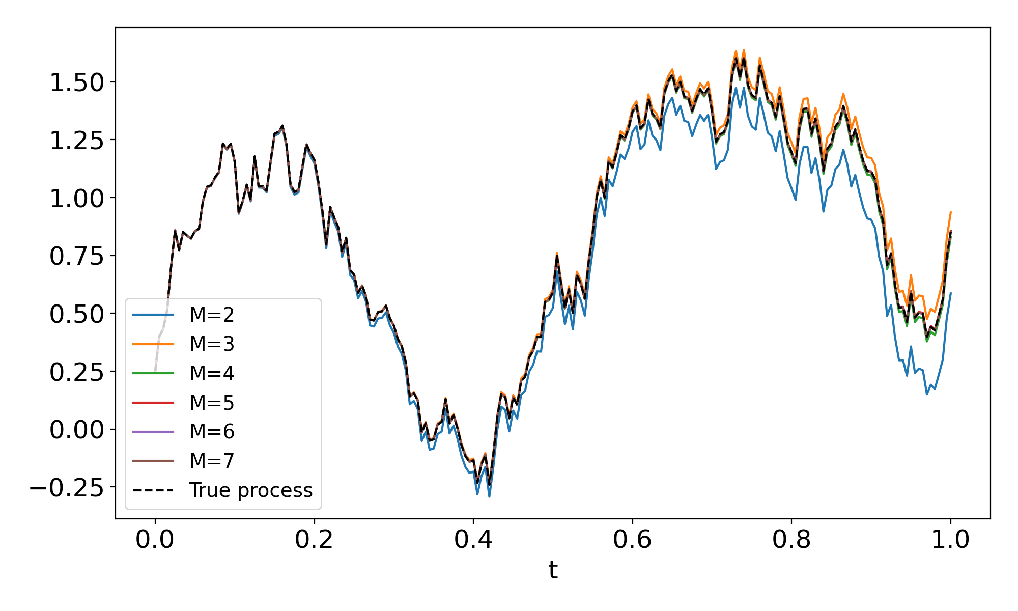
(a) $\kappa=1,\theta=0.25,\eta=1.2$

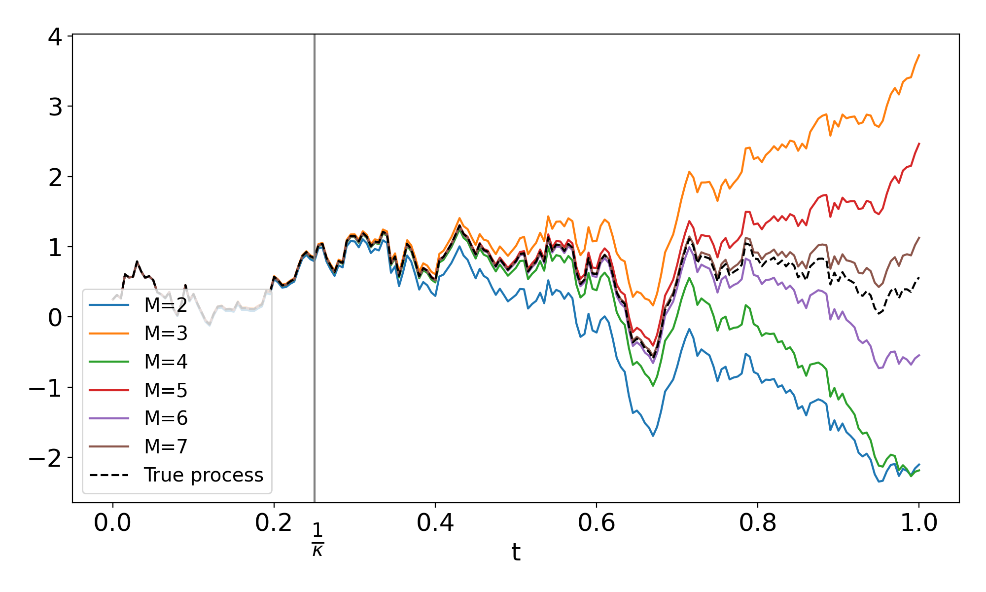
(b) $\kappa=4,\theta=0.25,\eta=2$

Figure 1: Trajectories of an Ornstein-Uhlenbeck process against their truncated time-independent linear representation (3.8), i.e. $\left\langle\bm{\ell}^{\textnormal{OU}},\widehat{\mathbb{W}}_{t}\right\rangle$, for several truncation orders $M$.

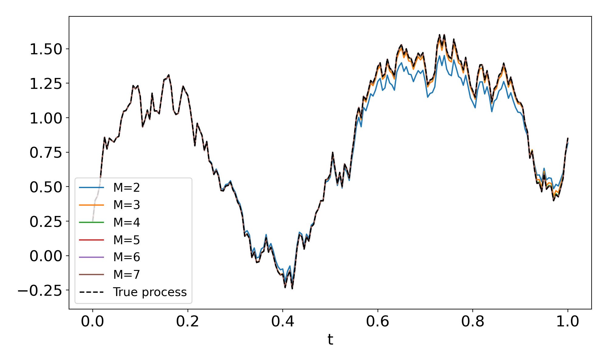
(a) $\kappa=1,\theta=0.25,\eta=1.2$

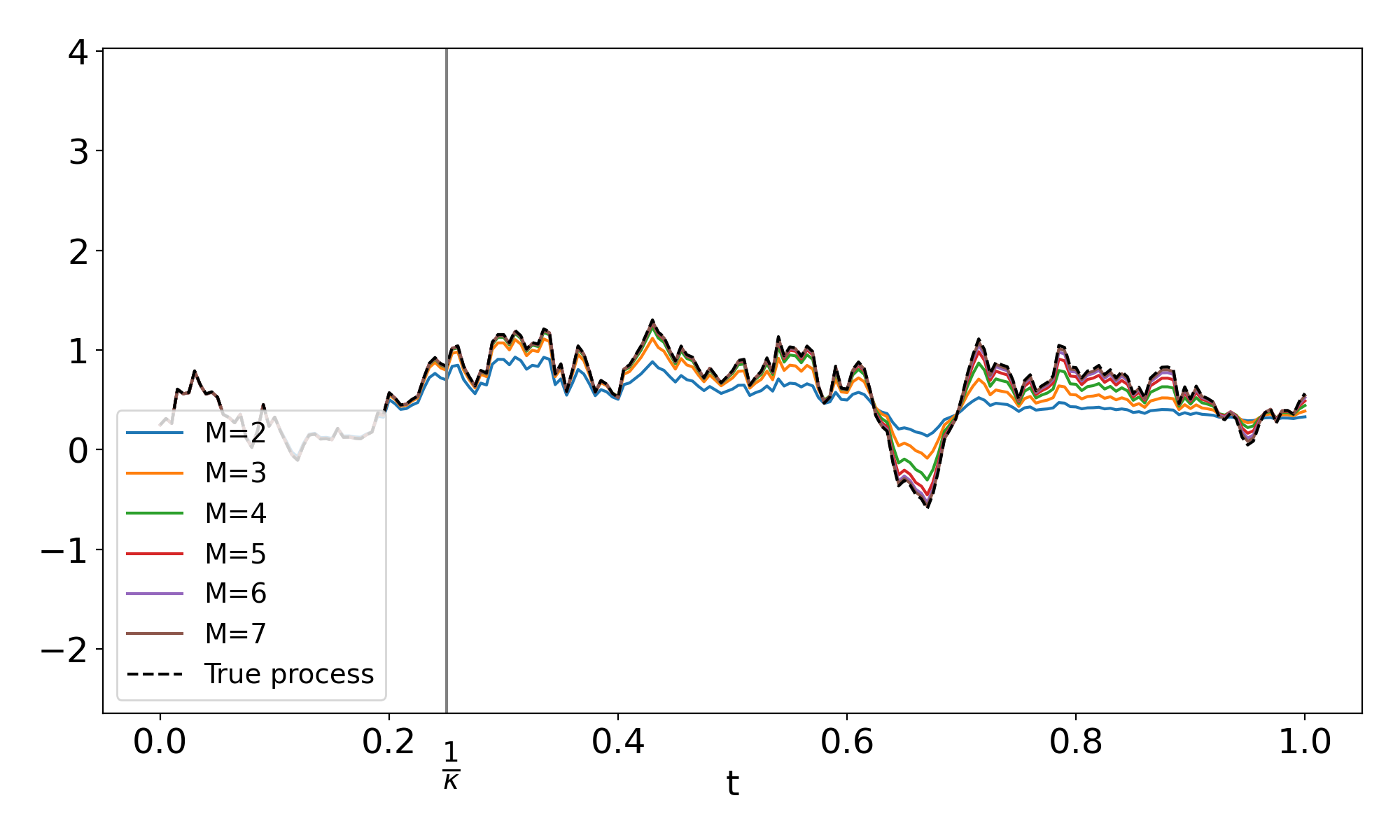
(b) $\kappa=4,\theta=0.25,\eta=2$

Figure 2: Trajectories of an Ornstein-Uhlenbeck process against their truncated time-dependent linear representation (3.9), i.e. $\left\langle\tilde{\bm{\ell}}_{t}^{\textnormal{OU}},\widehat{\mathbb{W}}_{t}\right\rangle$, for several truncation orders $M$.

If $|\kappa t|<1$, we can see in the left-hand side of Figure 1 and Figure 2 that the truncated linear representations seems to converge quite quickly to the explicit solution of the Ornstein-Uhlenbeck and a truncation order $M=4$ is sufficient to get a relatively close fit.

Going back to our signature volatility model, the representations of the Ornstein-Uhlenbeck process in Lemma 3.1 combined with the shuffle property of Proposition 2.6 show that the model (3.2)-(3.3) nests any stochastic volatility model based on an Ornstein-Uhlenbeck process of the form

$$\frac{dS_{t}}{S_{t}}=f(t,X_{t})dB_{t},\quad f(t,x)=\sum_{k\geq 0}\alpha_{k}(t)x^{k},$$

for some coefficients $\alpha_{k}:[0,T]\to\mathbb{R}$ that ensure the absolute convergence of the infinite sum. More precisely, using the representation (3.8) or (3.9) and the shuffle property in Lemma 2.6, we can write

$$f(t,X_{t})=\sum_{k\geq 0}\alpha_{k}(t)\left\langle\bm{\ell}^{\textnormal{OU}},\widehat{\mathbb{W}}_{t}\right\rangle^{k}=\left\langle\bm{\sigma}_{t},\widehat{\mathbb{W}}_{t}\right\rangle\quad\text{with }\bm{\sigma}_{t}:=\sum_{k\geq 0}\alpha_{k}(t)\left(\bm{\ell}^{\textnormal{OU}}\right)^{\mathrel{\sqcup\mkern-3.2mu\sqcup}k}.$$ (3.10)

This clearly includes:

• The Stein-Stein model [58] for $f(t,x)=x$,

• The Bergomi model [30, 15] for

  $$f(t,x)=\xi_{0}(t)e^{\eta x}=\xi_{0}(t)\sum_{k\geq 0}\frac{(\eta x)^{k}}{k!},$$

  for some $\eta\in\mathbb{R}$ and some deterministic input curve $\xi_{0}$,

• The Quintic OU model [4] for

  $$f(t,x)=\xi_{0}(t)(\alpha_{0}+\alpha_{1}x+\alpha_{3}x^{3}+\alpha_{5}x^{5}),$$

  for some $\alpha_{i}\geq 0$ and some deterministic input curve $\xi_{0}$, and any other finite polynomial of the Ornstein-Uhlenbeck process.

3.1.2 Models based on the mean-reverting geometric Brownian motion

More generally, the mean-reverting geometric Brownian motion (mGBM) $Y$, given by

$$dY_{t}=\kappa(\theta-Y_{t})dt+(\eta+\alpha Y_{t})dW_{t},\quad Y_{0}=y\in\mathbb{R},$$ (3.11)

for $\kappa,\theta,\eta,\alpha\in\mathbb{R}$ can be represented as an infinite linear combination of the signature of the time-extended Brownian motion, either in a time-independent or time-dependent way.

Lemma 3.2.

The unique solution $Y$ to (3.11) is given by

$$Y_{t}=\left\langle\bm{\ell}^{\textnormal{mGBM}},\widehat{\mathbb{W}}_{t}\right\rangle,\quad\bm{\ell}^{\textnormal{mGBM}}=\left(y{\color[rgb]{0.0600000000000001,0.46,1}\textup{{\o{}}}}+\left(\kappa\theta-\frac{\alpha\eta}{2}\right){\mathcolor{NavyBlue}{\mathbf{1}}}+\eta{\mathcolor{NavyBlue}{\mathbf{2}}}\right)e^{\mathrel{\sqcup\mkern-3.2mu\sqcup}\left(-\left(\kappa+\frac{\alpha^{2}}{2}\right){\mathcolor{NavyBlue}{\mathbf{1}}}+\alpha{\mathcolor{NavyBlue}{\mathbf{2}}}\right)},$$ (3.12)

such that $\bm{\ell}^{\textnormal{mGBM}}\in\mathcal{A}$, with $e^{\mathrel{\sqcup\mkern-3.2mu\sqcup}~{}}$ as defined in (2.9). Equivalently, $Y$ can also be written in terms of time-dependent coefficients:

$$Y_{t}=\left\langle\tilde{\bm{\ell}}_{t}^{\textnormal{mGBM}},\widehat{\mathbb{W}}_{t}\right\rangle,\quad\tilde{\bm{\ell}}_{t}^{\textnormal{mGBM}}=\theta{\color[rgb]{0.0600000000000001,0.46,1}\textup{{\o{}}}}+e^{-\lambda t}\left((\bm{\ell}^{\textnormal{mGBM}}-\theta{\color[rgb]{0.0600000000000001,0.46,1}\textup{{\o{}}}})\mathrel{\sqcup\mkern-3.2mu\sqcup}e^{\mathrel{\sqcup\mkern-3.2mu\sqcup}\lambda{\mathcolor{NavyBlue}{\mathbf{1}}}}\right),$$ (3.13)

for some $\lambda\in\mathbb{R}$.

Proof.

The proof is detailed in Appendix A.2. ∎

Example 3.2.1.

Up to order 3, the linear form of a mean-reverting geometric Brownian motion reads

$$\bm{\ell}^{\textnormal{mGBM}}=\left(y,\begin{pmatrix}\beta y+\gamma\\ \alpha y+\eta\end{pmatrix},\begin{pmatrix}(\beta y+\gamma)\beta&(\beta y+\gamma)\alpha\\ (\alpha y+\eta)\beta&(\alpha y+\eta)\alpha\end{pmatrix},\begin{pmatrix}(\beta y+\gamma)\beta^{2}&(\beta y+\gamma)\beta\alpha&\\ (\beta y+\gamma)\beta\alpha&(\beta y+\gamma)\alpha^{2}&\\ &(\alpha y+\eta)\beta^{2}&(\alpha y+\eta)\beta\alpha\\ &(\alpha y+\eta)\beta\alpha&(\alpha y+\eta)\alpha^{2}\end{pmatrix},\cdots\right),$$

where $\beta=-\left(\kappa+\frac{\alpha^{2}}{2}\right)$ and $\gamma=\kappa\theta-\frac{\alpha\eta}{2}$. $\blacksquare$

The behaviour and numerical limitations of the linear representations of the mean-reverting geometric Brownian motion are similar to those of the Ornstein-Uhlenbeck, as shown in Figure 3 and Figure 4.

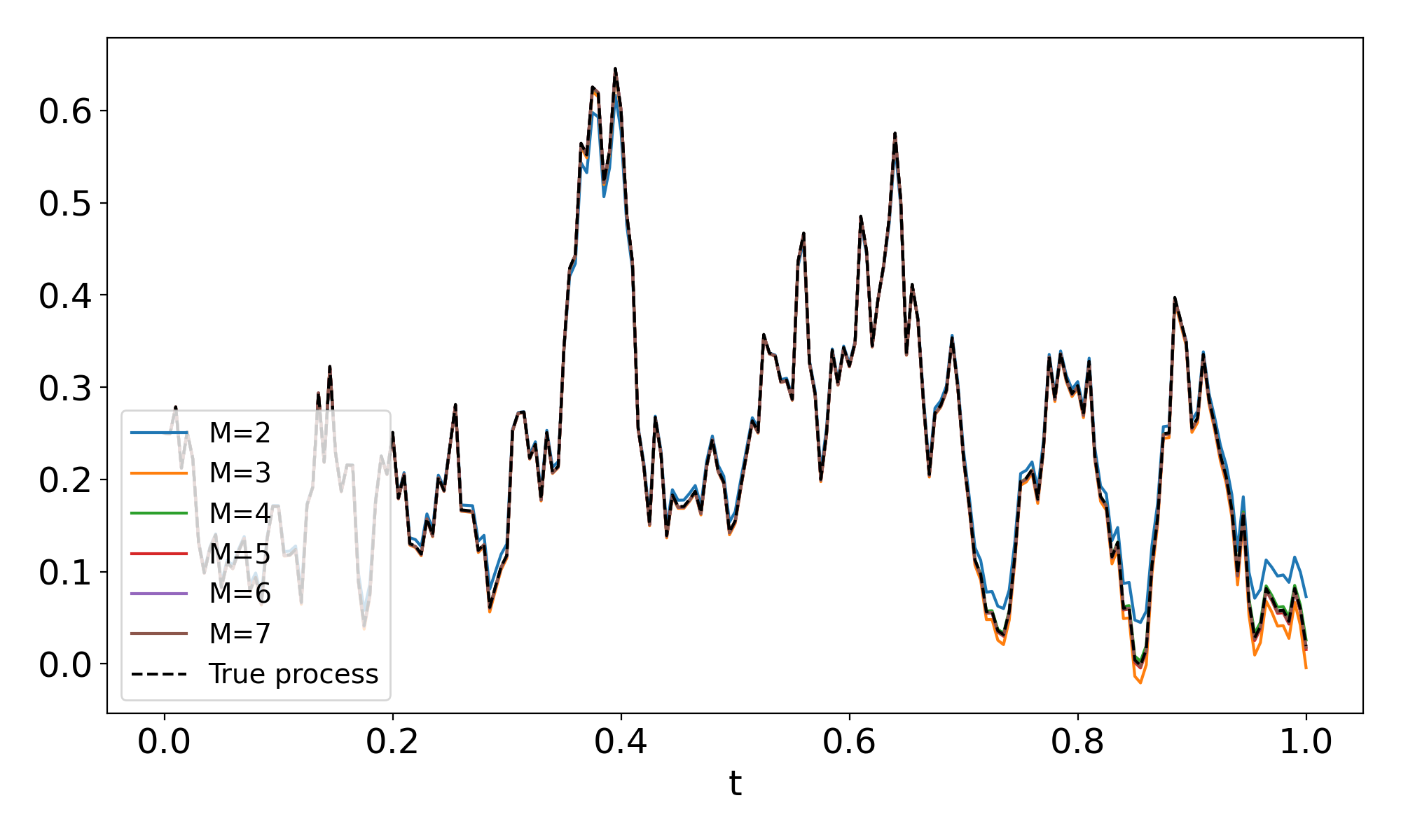
(a) $\kappa=1,\theta=0.25,\eta=0.5,\alpha=1.6$

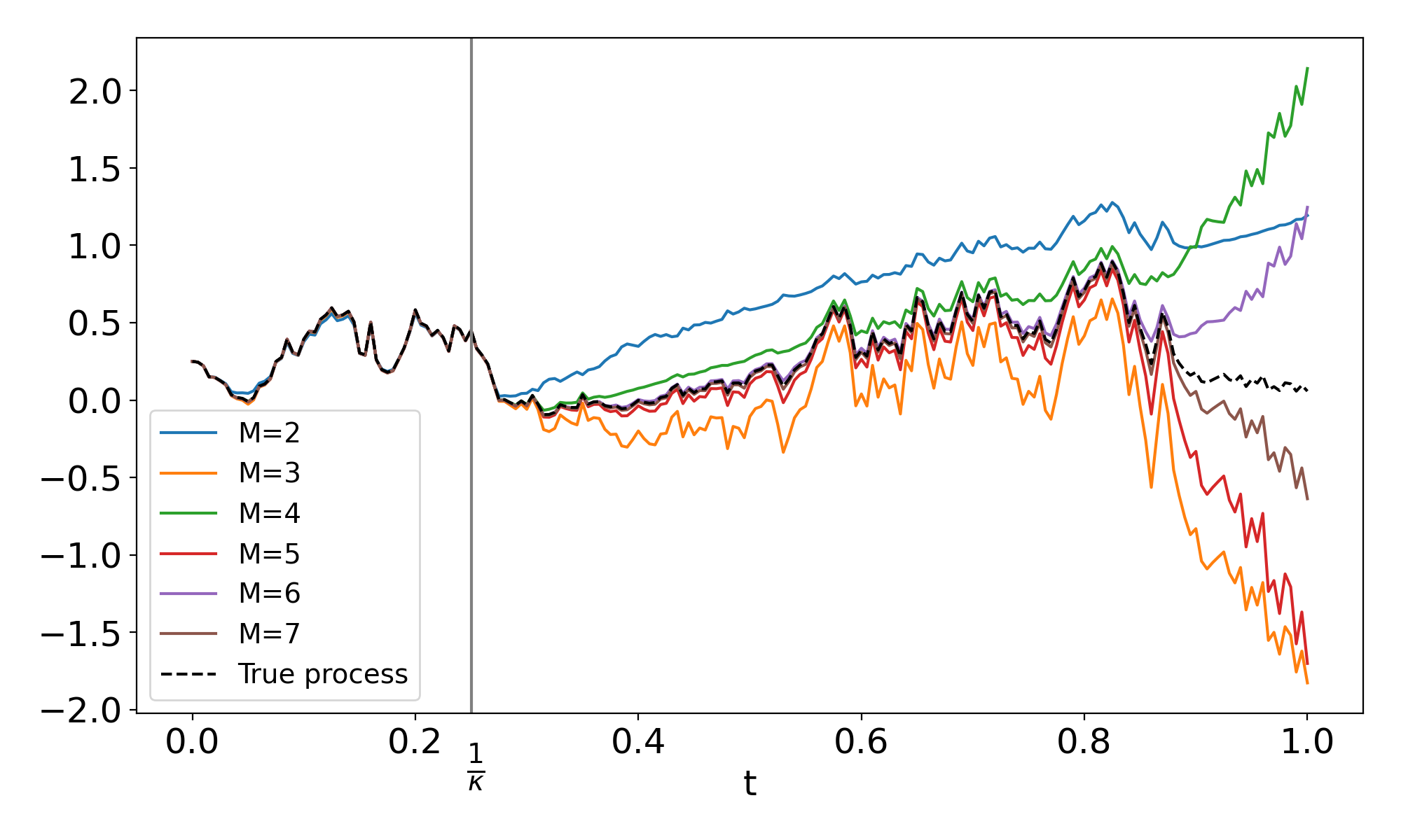
(b) $\kappa=4,\theta=0.25,\eta=0.5,\alpha=2$

Figure 3: Trajectories of a mean-reverting geometric Brownian motion against their truncated time-independent linear representation (3.12), i.e. $\left\langle\bm{\ell}^{\textnormal{mGBM}},\widehat{\mathbb{W}}_{t}\right\rangle$, for several truncation orders $M$.

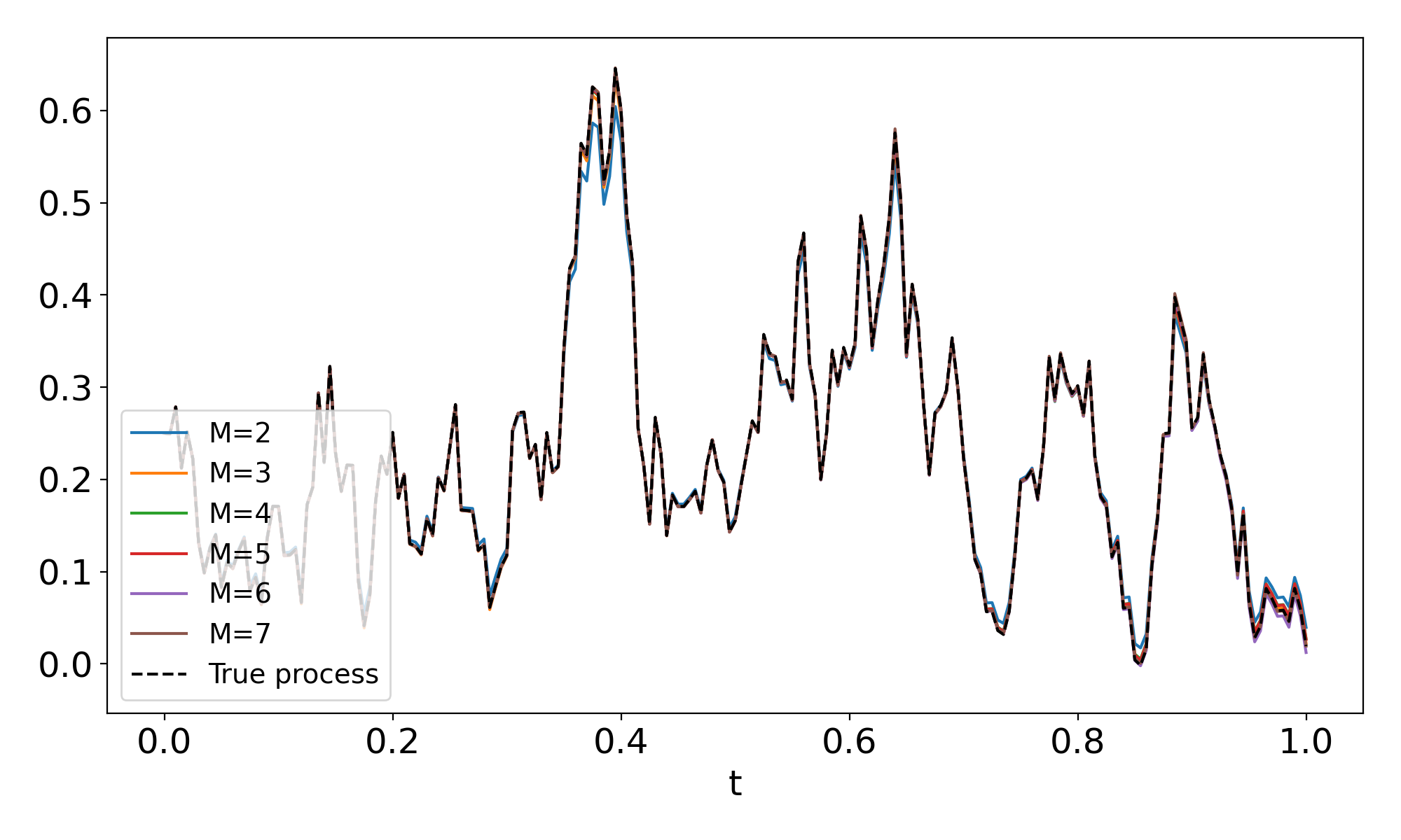
(a) $\kappa=1,\theta=0.25,\eta=0.5,\alpha=1.6,\lambda=0.3$

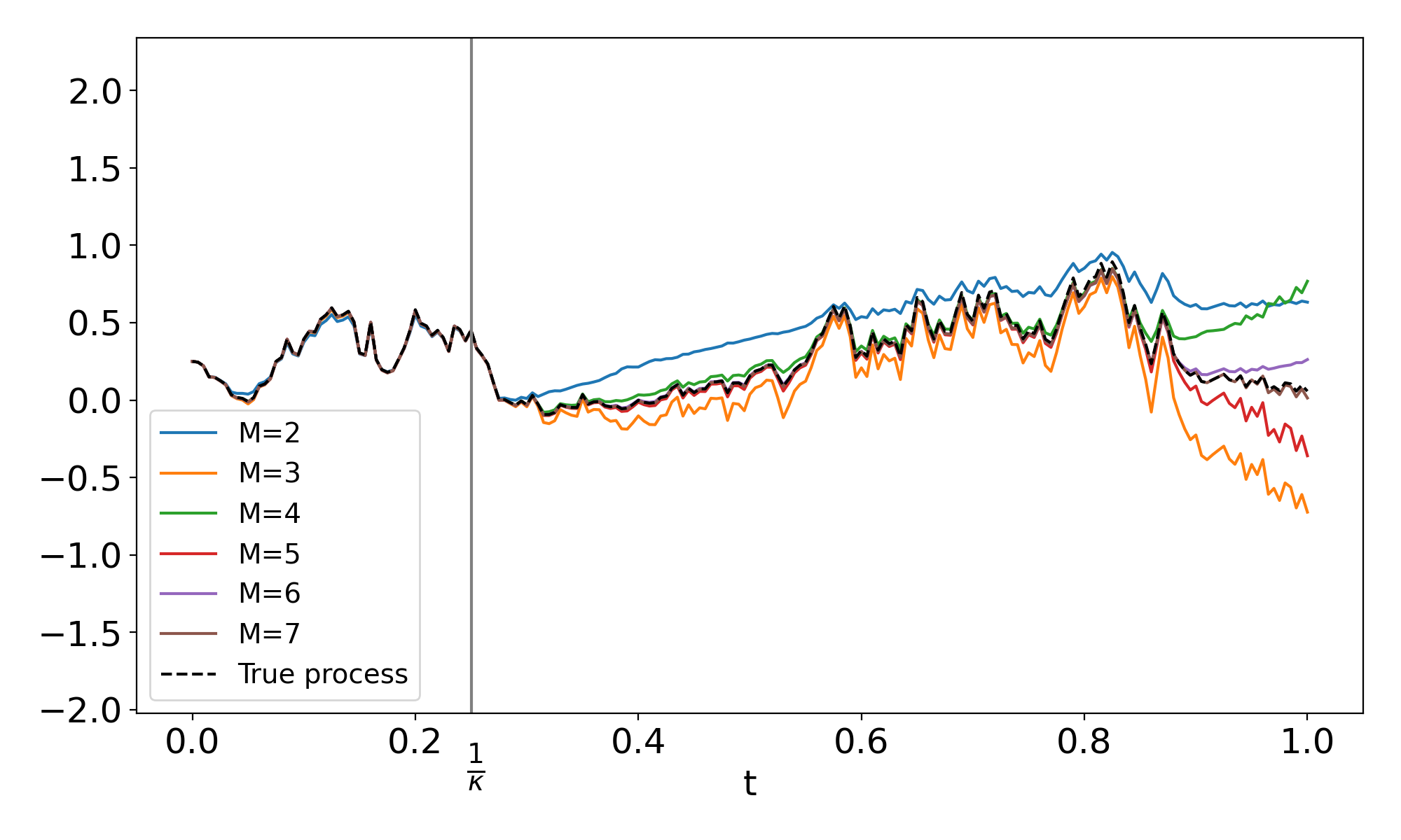
(b) $\kappa=4,\theta=0.25,\eta=0.5,\alpha=2,\lambda=0.5$

Figure 4: Trajectories of a mean-reverting geometric Brownian motion against their truncated time-dependent linear representation (3.13), i.e. $\left\langle\tilde{\bm{\ell}}_{t}^{\textnormal{mGBM}},\widehat{\mathbb{W}}_{t}\right\rangle$, for several truncation orders $M$.

Remark 3.2.1.

For Monte Carlo simulations, it is better to have explicit processes. When $\alpha\neq 0$, the mGBM solution to (3.11) can also be formulated explicitly with

$$Y_{t}:=\left(y+\frac{\eta}{\alpha}+\kappa\left(\theta+\frac{\eta}{\alpha}\right)\int_{0}^{t}e^{\left(\kappa+\frac{\alpha^{2}}{2}\right)s-\alpha W_{s}}ds\right)e^{-\left(\kappa+\frac{\alpha^{2}}{2}\right)t+\alpha W_{t}}-\frac{\eta}{\alpha}.$$ (3.14)

When $\alpha=0$, the mGBM is an Ornstein-Uhlenbeck process. $\blacksquare$

Going back to the signature volatility model (3.3). The mGBM representation encompasses the following volatility processes

• The volatility in the Hull-White model [43], i.e.

  $$\frac{d\sigma_{t}}{\sigma_{t}}=\left(\mu-\tfrac{1}{2}\xi^{2}\right)dt+\xi dW_{t},\quad\sigma_{0}\in\mathbb{R}.$$ (3.15)

• The volatility in Dupire [30], i.e.

  $$\frac{d\sigma_{t}}{\sigma_{t}}=\frac{1}{2}\left(\frac{\partial\log V_{t}(0)}{\partial t}-\frac{b^{2}}{4}\right)dt+\frac{b}{2}dW_{t},\quad\sigma_{0}\in\mathbb{R}^{+},$$ (3.16)

  for some deterministic forward variance curve $V_{t}(0)$. Note that the linear representation of $\sigma$ would be time-dependent.

3.1.3 Models based on the square-root process

A square-root or Cox-Ingersoll-Ross [24] (CIR) process $V$, driven by

$$dV_{t}=\kappa(\theta-V_{t})dt+\eta\sqrt{V_{t}}dW_{t},\quad V_{0}=v>0,$$ (3.17)

seems to admit a conjectured linear representation

$$V_{t}=\left\langle\bm{\ell}^{\textnormal{CIR}},\widehat{\mathbb{W}}_{t}\right\rangle=\left(\left\langle\bm{\sigma}^{\textnormal{CIR}},\widehat{\mathbb{W}}_{t}\right\rangle\right)^{2},$$ (3.18)

where $\bm{\ell}^{\textnormal{CIR}}:=(\bm{\sigma}^{\textnormal{CIR}})^{\mathrel{\sqcup\mkern-3.2mu\sqcup}2}$ with $\bm{\sigma}^{\textnormal{CIR}}$ satisfying the non-linear algebraic equation

$$(\bm{\sigma}^{\textnormal{CIR}})^{\mathrel{\sqcup\mkern-3.2mu\sqcup}2}=v{\color[rgb]{0.0600000000000001,0.46,1}\textup{{\o{}}}}+\left(\left(\kappa\theta-\frac{\eta^{2}}{4}\right){\color[rgb]{0.0600000000000001,0.46,1}\textup{{\o{}}}}-\kappa(\bm{\sigma}^{\textnormal{CIR}})^{\mathrel{\sqcup\mkern-3.2mu\sqcup}2}\right){\mathcolor{NavyBlue}{\mathbf{1}}}+\eta\bm{\sigma}^{\textnormal{CIR}}{\mathcolor{NavyBlue}{\mathbf{2}}}.$$

The theoretical convergence, i.e. proving that $\bm{\sigma}^{\textnormal{CIR}}\in\mathcal{A}$, seems intricate to obtain but is ongoing in a separate work. From the numerical perspective, Figure 5 seems to validate our formula under the Feller condition $2\kappa\theta>\eta$ [34]. Figure 15 below also provides a numerical convergence of prices of our representation (3.18) in the context of the Heston model.

Example 3.2.2.

Up to order 3, the linear representation of the Cox-Ingersoll-Ross process reads

$$\bm{\ell}^{\textnormal{CIR}} =\left(v,\begin{pmatrix}\beta\\ \alpha\end{pmatrix},\begin{pmatrix}-\kappa\beta&\lambda\beta\\ -\kappa\alpha&\lambda\alpha\end{pmatrix},\begin{pmatrix}\kappa^{2}\beta&-\left(\kappa+\frac{\beta}{2v}\right)\lambda\beta&\\ -\kappa\lambda\beta&0&\\ &\kappa^{2}\alpha&-\left(\kappa+\frac{\beta}{2v}\right)\lambda\alpha\\ &-\kappa\lambda\alpha&0\end{pmatrix},\cdots\right),$$

where $\beta:=-\kappa(v-\theta)-\frac{\eta^{2}}{4},\alpha:=\eta\sqrt{v}$ and $\lambda:=\frac{\eta}{2\sqrt{v}}$. $\blacksquare$

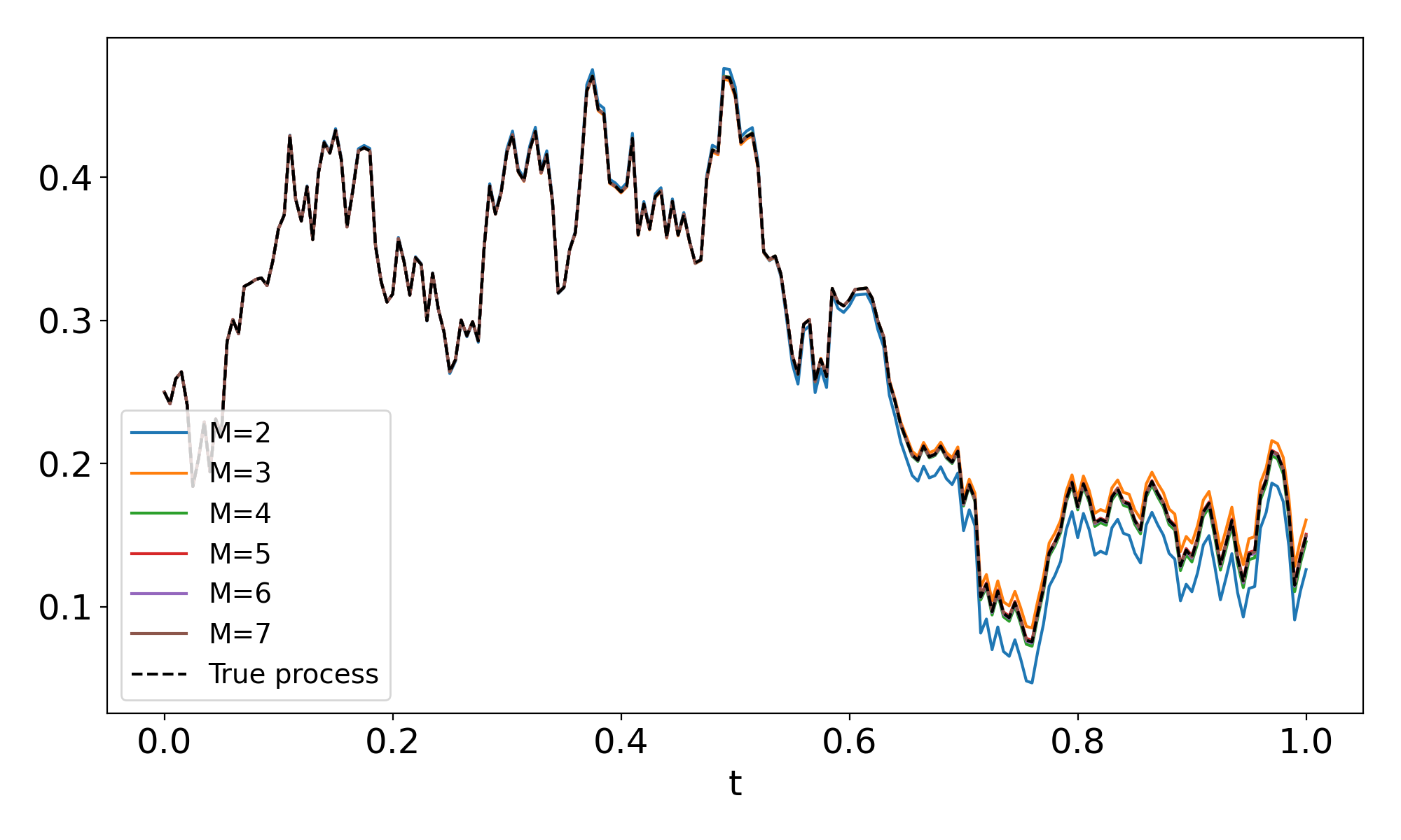
(a) $\kappa=1,\theta=0.25,\eta=0.7$

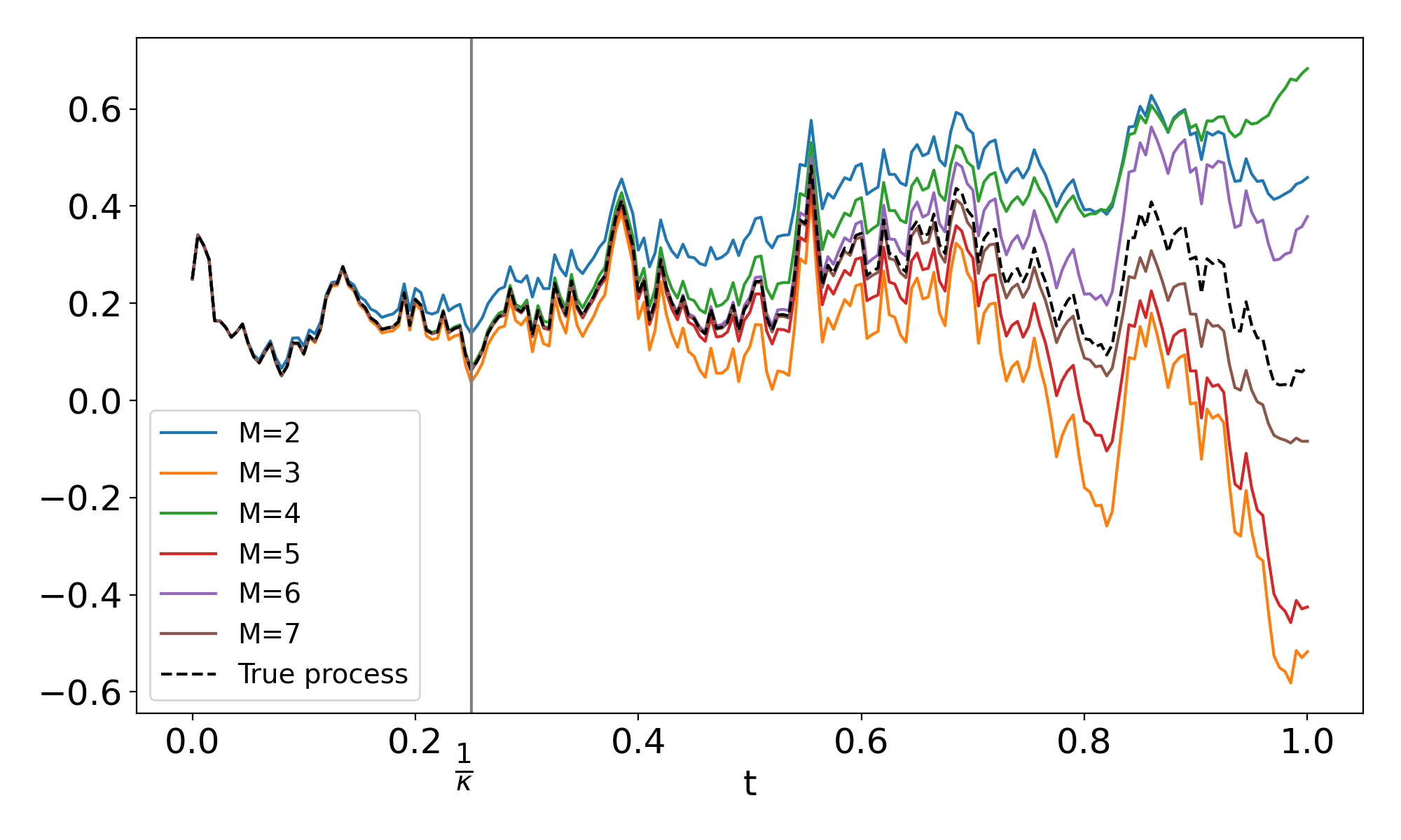
(b) $\kappa=4,\theta=0.25,\eta=1.4$

Figure 5: Trajectories of a Cox-Ingersoll-Ross process against their truncated time-independent linear representation (3.18), i.e. $\left\langle\bm{\ell}^{\textnormal{CIR}},\widehat{\mathbb{W}}_{t}\right\rangle$, for several truncation orders $M$.

Going back to our signature volatility model, the representation (3.18) allows us to include in our framework the volatility of the Heston model [42].

3.1.4 Models based on path-dependent processes

As shown in [6], several path-dependent stochastic Volterra processes:

$$Z_{t}=Z_{0}+\int_{0}^{t}K(t-s)(a_{0}+a_{1}Z_{s})ds+\int_{0}^{t}K(t-s)(b_{0}+b_{1}Z_{s})dW_{s},$$

with $Z_{0},a_{0},a_{1},b_{0},b_{1}\in\mathbb{R}$, for certain locally square-integrable kernels $K$ also admit linear representations in the form $Z_{t}=\left\langle\bm{\ell}_{t},\widehat{\mathbb{W}}_{t}\right\rangle$. This includes non-semimartingale processes such as the Riemann-Liouville fractional Brownian motion

$$W_{t}^{H}=\int_{0}^{t}(t-s)^{H-1/2}dW_{s},\quad H\in(0,1).$$

For instance, the (time-dependent) representation of $W^{H}$ reads

$$W_{t}^{H}=\left\langle\bm{\ell}_{t}^{\textnormal{RL}},\widehat{\mathbb{W}}_{t}\right\rangle,\quad\bm{\ell}_{t}^{\textnormal{RL}}=t^{H-\frac{1}{2}}\sum_{n=0}^{\infty}\frac{\left(\frac{1}{2}-H\right)^{\bar{n}}}{t^{n}}{\mathcolor{NavyBlue}{\mathbf{1}}}^{\otimes n}{\mathcolor{NavyBlue}{\mathbf{2}}},$$

where $(\cdot)^{\bar{n}}$ is the rising factorial. Please refer to [6, Section 4] for more details on such representations. Again any volatility process that is an analytic function of such processes falls into the framework of signature volatility models (3.2)-(3.3) thanks to the shuffle property, recall (3.10). This includes for instance the class of Volterra polynomial models [5], in particular Volterra [2] and rough Bergomi models [12].

As as final example, the delayed equation (DE) process $U$, given by

$$dU_{t} =\left(a+\int_{0}^{t}e^{\alpha(t-s)}U_{s}ds\right)dt+\left(b+\int_{0}^{t}e^{\beta(t-s)}U_{s}ds\right)dW_{t},\quad U_{0}=u\in\mathbb{R},$$ (3.19)

for some $a,b,\alpha,\beta\in\mathbb{R}$, can be represented as a linear combination of the signature of the time-extended Brownian motion with

$$U_{t}=\left\langle\bm{\ell}^{\textnormal{DE}},\widehat{\mathbb{W}}_{t}\right\rangle,\quad\bm{\ell}^{\textnormal{DE}}=(u{\color[rgb]{0.0600000000000001,0.46,1}\textup{{\o{}}}}+a{\mathcolor{NavyBlue}{\mathbf{1}}}+b{\mathcolor{NavyBlue}{\mathbf{2}}})\left({\color[rgb]{0.0600000000000001,0.46,1}\textup{{\o{}}}}-{\mathcolor{NavyBlue}{\mathbf{1}}}\left(e^{\mathrel{\sqcup\mkern-3.2mu\sqcup}\alpha{\mathcolor{NavyBlue}{\mathbf{1}}}}{\mathcolor{NavyBlue}{\mathbf{1}}}+e^{\mathrel{\sqcup\mkern-3.2mu\sqcup}\beta{\mathcolor{NavyBlue}{\mathbf{1}}}}{\mathcolor{NavyBlue}{\mathbf{2}}}\right)\right)^{-1}.$$ (3.20)

The reader can refer to [6, Theorem 4.4] for more details on the linear delayed equation process.

Example 3.2.3.

Up to order 3, the linear form of a delayed equation process reads

$$\bm{\ell}^{\textnormal{DE}}=\left(x,\begin{pmatrix}a\\ b\end{pmatrix},\begin{pmatrix}z&z\\ 0&0\end{pmatrix},\begin{pmatrix}\alpha z+a&\beta z+a&\\ 0&0&\\ &b&b\\ &0&0\end{pmatrix},\cdots\right),$$

see Figure 6 for a numerical illustration of the signature representation. $\blacksquare$

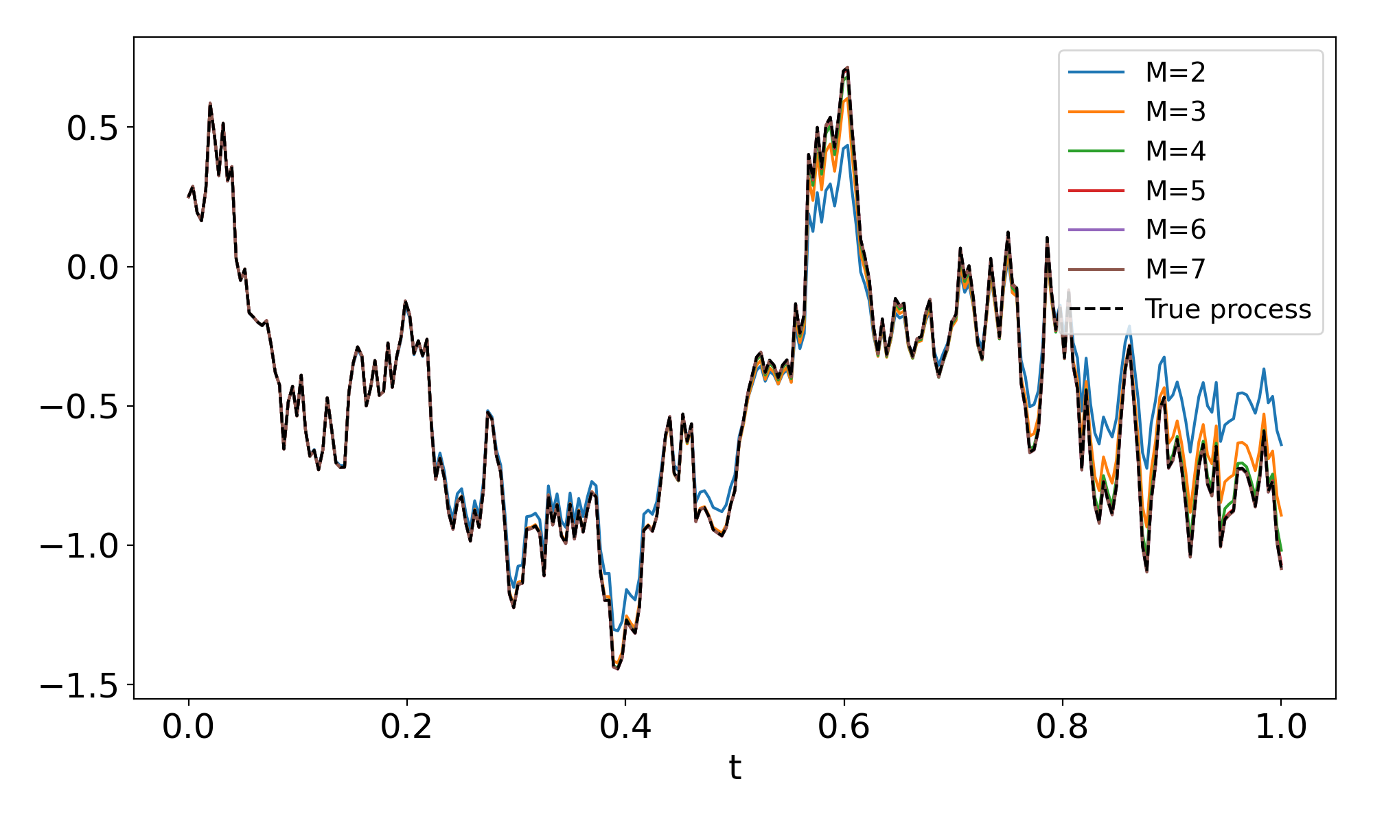
(a) $a=-2,b=-0.5,z=0.25,\alpha=1,\beta=1.5$

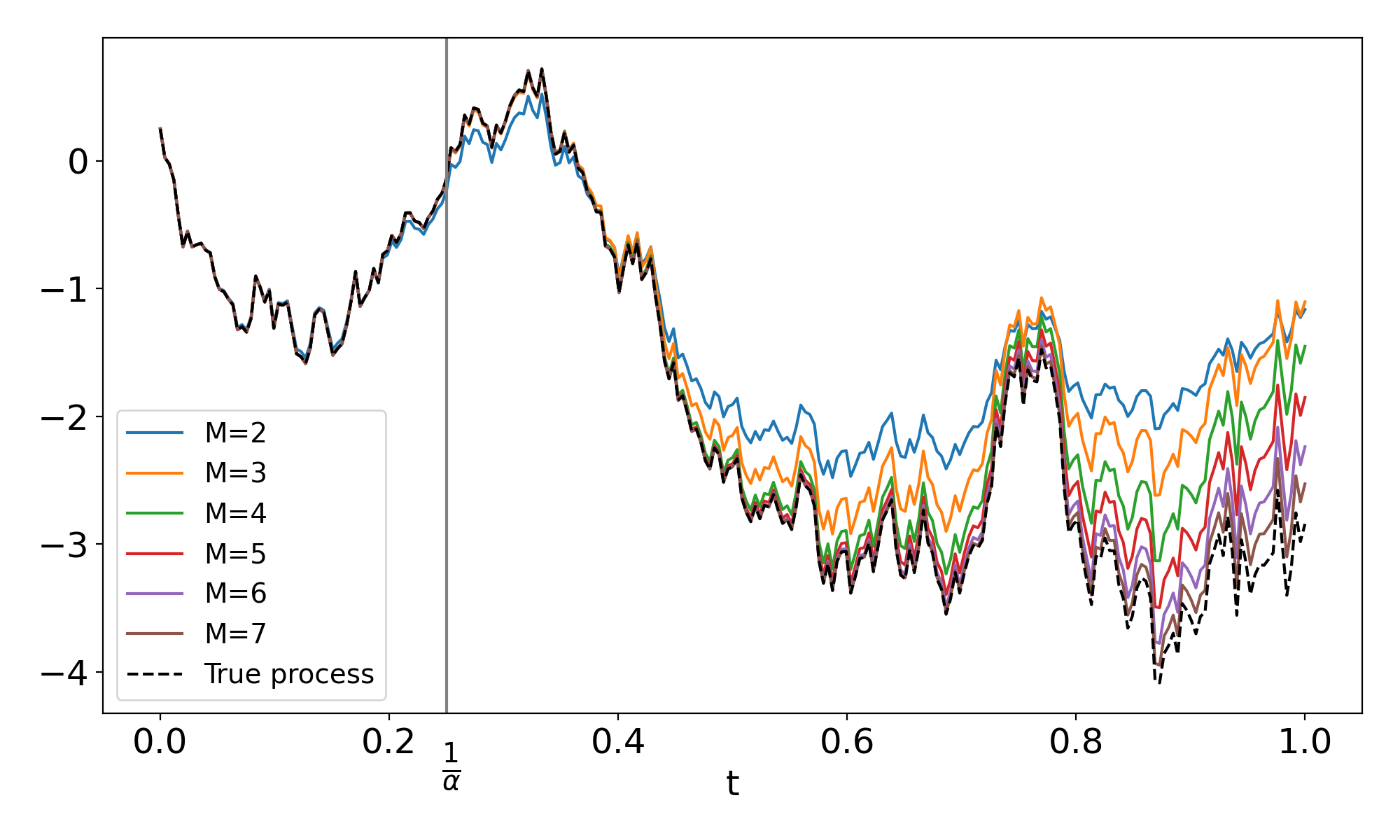
(b) $a=-2,b=-0.5,z=0.25,\alpha=4,\beta=1.5$

Figure 6: Trajectories of a delayed equation process against their truncated time-independent linear representation (3.20), i.e. $\left\langle\bm{\ell}^{\textnormal{DE}},\widehat{\mathbb{W}}_{t}\right\rangle$, for several truncation orders $M$.

3.2 Leverage effect

The leverage effect in the model (3.2)-(3.3) is defined as the instantaneous correlation between the log-price $S$ and its instantaneous volatility $|\Sigma|$ defined by

$$\frac{d[\log S,|\Sigma|]_{t}}{\sqrt{d[\log S]_{t}}\sqrt{d[|\Sigma|]_{t}}}.$$

In practice, the leverage effect is negative on equity markets and one usually would like to control its sign via the correlation parameter $\rho$ between $B$ and $W$ in (3.1). Since $\Sigma$ is not necessarily positive at all time, the leverage effect can flip sign in the model (3.2)-(3.3), which is not realistic. The next Lemma provides a necessary and sufficient condition on the coefficients $\bm{\sigma}$ for the leverage effect to be equal to $\rho$, at all time.

Lemma 3.3.

Assume $\bm{\sigma}\in\mathcal{I}^{\prime}$, then the leverage effect is given by

$$\frac{d[\log S,|\Sigma|]_{t}}{\sqrt{d[\log S]_{t}}\sqrt{d[|\Sigma|]_{t}}}=\rho\,\textnormal{sign}\left(\left\langle\bm{\sigma}_{t}|_{{\mathcolor{NavyBlue}{\mathbf{2}}}},\widehat{\mathbb{W}}_{t}\right\rangle\right),$$

where $\textnormal{sign}(x)=1$ if $x\geq 0$ and $-1$ otherwise. In particular, it is equal to $\rho$ for all $t\geq 0$ if and only if $\bm{\sigma}$ satisfies

$$\left\langle\bm{\sigma}_{t}|_{{\mathcolor{NavyBlue}{\mathbf{2}}}},\widehat{\mathbb{W}}_{t}\right\rangle\geq 0,\quad t\geq 0.$$ (3.21)

Proof.

The dynamics of $\log S$ are in the form

$$d\log S_{t}=-\frac{1}{2}\Sigma_{t}^{2}dt+\Sigma_{t}dB_{t}=-\frac{1}{2}\left\langle\bm{\sigma}_{t}^{\mathrel{\sqcup\mkern-3.2mu\sqcup}2},\widehat{\mathbb{W}}_{t}\right\rangle dt+\left\langle\bm{\sigma}_{t},\widehat{\mathbb{W}}_{t}\right\rangle dB_{t}.$$ (3.22)

The instantaneous volatility of the model is $|\Sigma|$. By an application of Itô-Tanaka’s formula on $|\Sigma|$ and of Lemma 2.7, we have

$$d|\Sigma|_{t} =\textnormal{sign}\left(\Sigma_{t}\right)d\Sigma_{t}+dL^{0}(t)$$

$$=\textnormal{sign}\left(\Sigma_{t}\right)\left\langle\bm{\sigma}_{t}|_{{\mathcolor{NavyBlue}{\mathbf{2}}}},\widehat{\mathbb{W}}_{t}\right\rangle dW_{t}+\textnormal{sign}\left(\Sigma_{t}\right)\left\langle\bm{\sigma}_{t}|_{{\mathcolor{NavyBlue}{\mathbf{1}}}}+\tfrac{1}{2}\bm{\sigma}_{t}|_{{\mathcolor{NavyBlue}{\mathbf{22}}}}+\dot{\bm{\sigma}}_{t},\widehat{\mathbb{W}}_{t}\right\rangle dt+dL^{0}(t),$$

where $L^{0}$ is the local time of $\Sigma$ at 0. It follows that the leverage effect is given by

$$\frac{d[\log S,|\Sigma|]_{t}}{\sqrt{d[\log S]_{t}}\sqrt{d[|\Sigma|]_{t}}}=\rho\frac{\Sigma_{t}\,\textnormal{sign}\left(\Sigma_{t}\right)\left\langle\bm{\sigma}_{t}|_{{\mathcolor{NavyBlue}{\mathbf{2}}}},\widehat{\mathbb{W}}_{t}\right\rangle}{|\Sigma_{t}|\left|\left\langle\bm{\sigma}_{t}|_{{\mathcolor{NavyBlue}{\mathbf{2}}}},\widehat{\mathbb{W}}_{t}\right\rangle\right|}=\rho\,\textnormal{sign}\left(\left\langle\bm{\sigma}_{t}|_{{\mathcolor{NavyBlue}{\mathbf{2}}}},\widehat{\mathbb{W}}_{t}\right\rangle\right).$$

∎

The condition (3.21) can be made explicit in the Stein-Stein, Quintic and Bergomi models as shown in the next example.

Example 3.3.1.

• For the Stein-Stein model driven by a Brownian motion, $\bm{\sigma}|_{{\mathcolor{NavyBlue}{\mathbf{2}}}}=\eta{\color[rgb]{0.0600000000000001,0.46,1}\textup{{\o{}}}}$, see (3.8), and $\left\langle\bm{\sigma}|_{{\mathcolor{NavyBlue}{\mathbf{2}}}},\widehat{\mathbb{W}}_{t}\right\rangle=\eta\geq 0$,

• For the Quintic model of [4] constructed on a Brownian motion, $\bm{\sigma}=\alpha_{0}{\color[rgb]{0.0600000000000001,0.46,1}\textup{{\o{}}}}+\alpha_{1}{\mathcolor{NavyBlue}{\mathbf{2}}}+\alpha_{3}{\mathcolor{NavyBlue}{\mathbf{222}}}+\alpha_{5}{\mathcolor{NavyBlue}{\mathbf{22222}}}$ so that $\bm{\sigma}|_{{\mathcolor{NavyBlue}{\mathbf{2}}}}=\alpha_{1}{\color[rgb]{0.0600000000000001,0.46,1}\textup{{\o{}}}}+\alpha_{3}{\mathcolor{NavyBlue}{\mathbf{22}}}+\alpha_{5}{\mathcolor{NavyBlue}{\mathbf{2222}}}$, which gives

  $$\left\langle\bm{\sigma}|_{{\mathcolor{NavyBlue}{\mathbf{2}}}},\widehat{\mathbb{W}}_{t}\right\rangle=\alpha_{1}+\frac{\alpha_{3}}{2}W^{2}_{t}+\frac{\alpha_{5}}{4!}W^{4}_{t}\geq 0,\quad t\geq 0,$$

  as long as $\alpha_{1},\alpha_{3},\alpha_{5}$ are non negative,

• For the Bergomi model, see [30, 15], $\bm{\sigma}_{t}=\xi_{0}(t)e^{\mathrel{\sqcup\mkern-3.2mu\sqcup}\eta{\mathcolor{NavyBlue}{\mathbf{2}}}}$ so that $\bm{\sigma}_{t}|_{{\mathcolor{NavyBlue}{\mathbf{2}}}}=\eta\xi_{0}(t)e^{\mathrel{\sqcup\mkern-3.2mu\sqcup}\eta{\mathcolor{NavyBlue}{\mathbf{2}}}}$, which gives

  $$\left\langle\bm{\sigma}_{t}|_{{\mathcolor{NavyBlue}{\mathbf{2}}}},\widehat{\mathbb{W}}_{t}\right\rangle=\eta\xi_{0}(t)e^{\eta W_{t}}\geq 0,$$

  as long as $\xi_{0}(t),\eta$ are non negative, for all $t\leq T$.

$\blacksquare$

3.3 Approximated representations

More generally, if exact linear representations are not available for certain processes, approximate representations can be obtained thanks to the universal approximation property of path-signatures:

Theorem 3.4 (Universal approximation theorem [27]).

For some $t\in[0,T]$, let $K_{t}$ be a compact subset of $\{(\widehat{\mathbb{W}}_{s}^{\leq 2})_{s\in[0,t]}(\omega):\omega\in\Omega\}$ and consider a continuous map $F:K_{t}\to\mathbb{R}$. Then for every $\epsilon>0$, there exists some $M^{\epsilon}\in\mathbb{N}$ and some $\bm{f}^{\epsilon}\in T^{M^{\epsilon}}(\mathbb{R}^{2})$ such that

$$\sup_{W\in K_{t}}\left|F\left((\widehat{\mathbb{W}}_{s}^{\leq 2})_{s\in[0,t]}\right)-\left\langle\bm{f}^{\epsilon},\widehat{\mathbb{W}}_{t}\right\rangle\right|<\epsilon,$$

almost surely.

In practice, one would perform a linear regression on trajectories of a given process $X$ against a finite linear combination of the signature elements using the following steps:

Algorithm 3.5 (Regression against truncated signature).

Assume the spot volatility is of the following form

$$X_{t}=F(t,(W_{s})_{s\leq t}).$$

1. Generate $N$ realizations of the Brownian motion $W$, denoted by $W^{(1)},\ldots,W^{(N)}$,

2. For each realization $n=1,\ldots,N$, compute $X^{(n)}$ and the truncated signature $\widehat{\mathbb{W}}_{~{}}^{(n),\leq M}$ up to order $M$,

3. Regress $\left(X^{(1)},\ldots,X^{(N)}\right)$ against $\left(\widehat{\mathbb{W}}_{~{}}^{(1),\leq M},\ldots,\widehat{\mathbb{W}}_{~{}}^{(N),\leq M}\right)$ with $L^{1}$ and $L^{2}$ regularization $\beta_{1}$ and $\beta_{2}$ to learn the coefficients of $\bm{f}$ that minimize

   $$\min_{\bm{f}\in T^{M}(\mathbb{R}^{d})}\frac{1}{N}\frac{1}{J}\sum_{n=1}^{N}\sum_{j=1}^{J}\left|X^{(n)}_{t_{j}}-\left\langle\bm{f},\widehat{\mathbb{W}}_{t_{j}}^{(n),\leq M}\right\rangle\right|^{2}+\sum_{k=0}^{M}\sum_{{\mathcolor{NavyBlue}{\mathbf{v}}}\in V_{k}}\left(\beta_{1}\left|\bm{\ell}^{{\mathcolor{NavyBlue}{\mathbf{i_{1}\cdots i_{k}}}}}\right|+\beta_{2}\left(\bm{\ell}^{{\mathcolor{NavyBlue}{\mathbf{i_{1}\cdots i_{k}}}}}\right)^{2}\right).$$

Such approach appeared in Cuchiero et al. [27], Lyons et al. [48], Fermanian [36], Arribas et al. [10].

(a) $T=0.25$.

(b) $T=2$.

Figure 7: Trajectories of an inverse CIR process against their linear regression. $\kappa=4,\theta=0.5,\eta=2$

We recall the dynamics of the inverse CIR process, being the variance in the 3/2 model [52], driven by

$$dV_{t}=\kappa V_{t}(\theta-V_{t})dt+\eta V_{t}^{\frac{3}{2}}dW_{t}.$$

We see in Figure 7 that a process without known linear representation can still be approximated quite well through a linear regression.

(a) $H=0.1$.

(b) $H=0.3$.

Figure 8: Trajectories of a fractional Brownian motion against their linear regression for $M=6$.

However, as shown on Figure 8, the regression approach does not always work with small truncation levels. For instance, the ability to capture high roughness in a linear functional is not trivial to achieve whilst keeping the natural embedding $\widehat{W}_{t}=(t,W_{t})$.

We end this section with a brief comparison of approximate vs exact representations. As seen in the previous subsections, the convergence of the linear representation is quick for short horizons. However, when the horizon gets too large, relatively to the parameters of the represented models, e.g. the mean reversion rate, the truncated representations drastically deteriorates, see Figures 1 to 6. Yet, as seen previously, linear regressions make quite stable representations over their training time and can thus be made over targeted horizons to control the stability. In Figures 9, 10 and 11, we can remark that for short horizons (relative to $\kappa$), the linear regression doesn’t fit as well as the linear representation. However for longer horizons, where the linear representation lacks in stability, the linear regression retains hers.

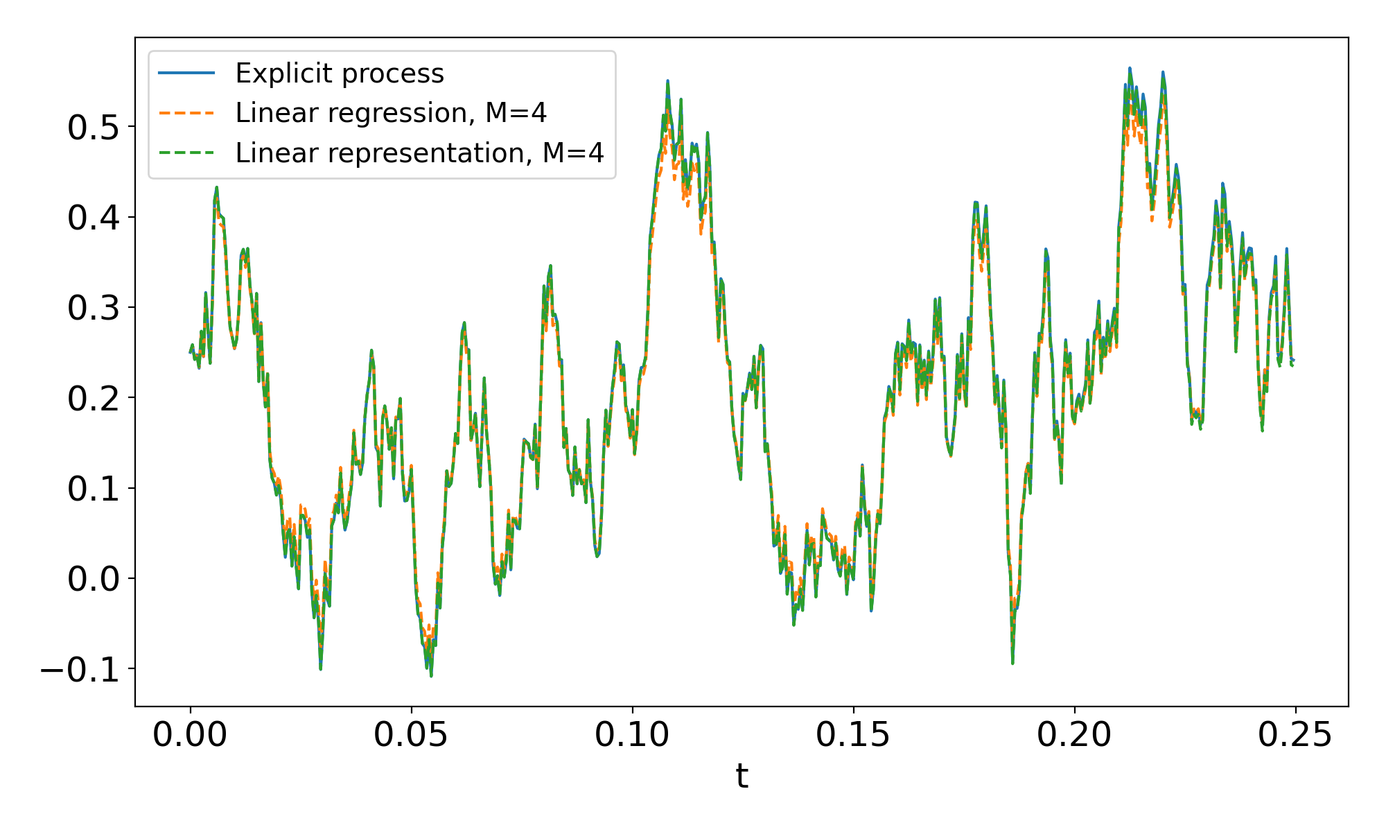
(a) $T=0.25$.

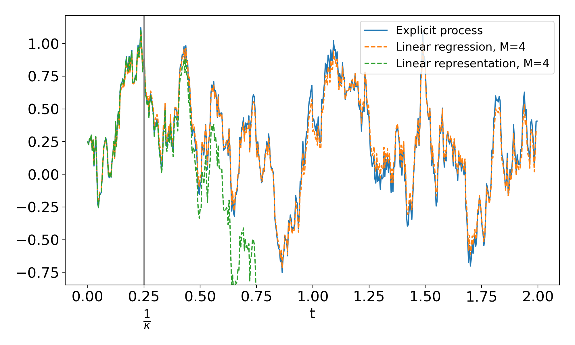
(b) $T=2$.

Figure 9: Trajectories of an Ornstein-Uhlenbeck process against their linear representation and linear regression. $\kappa=4,\theta=0.25,\eta=2$

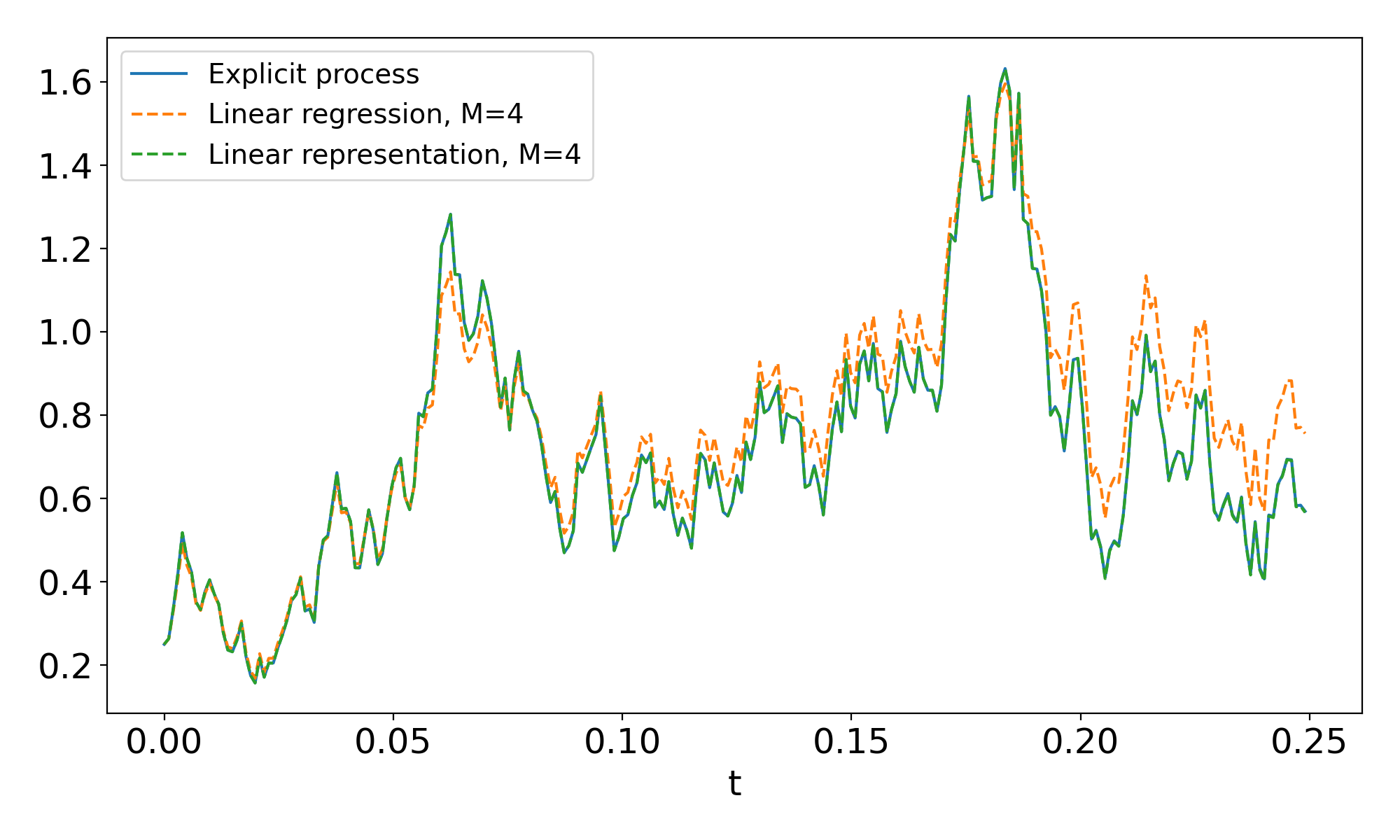
(a) $T=0.25$.

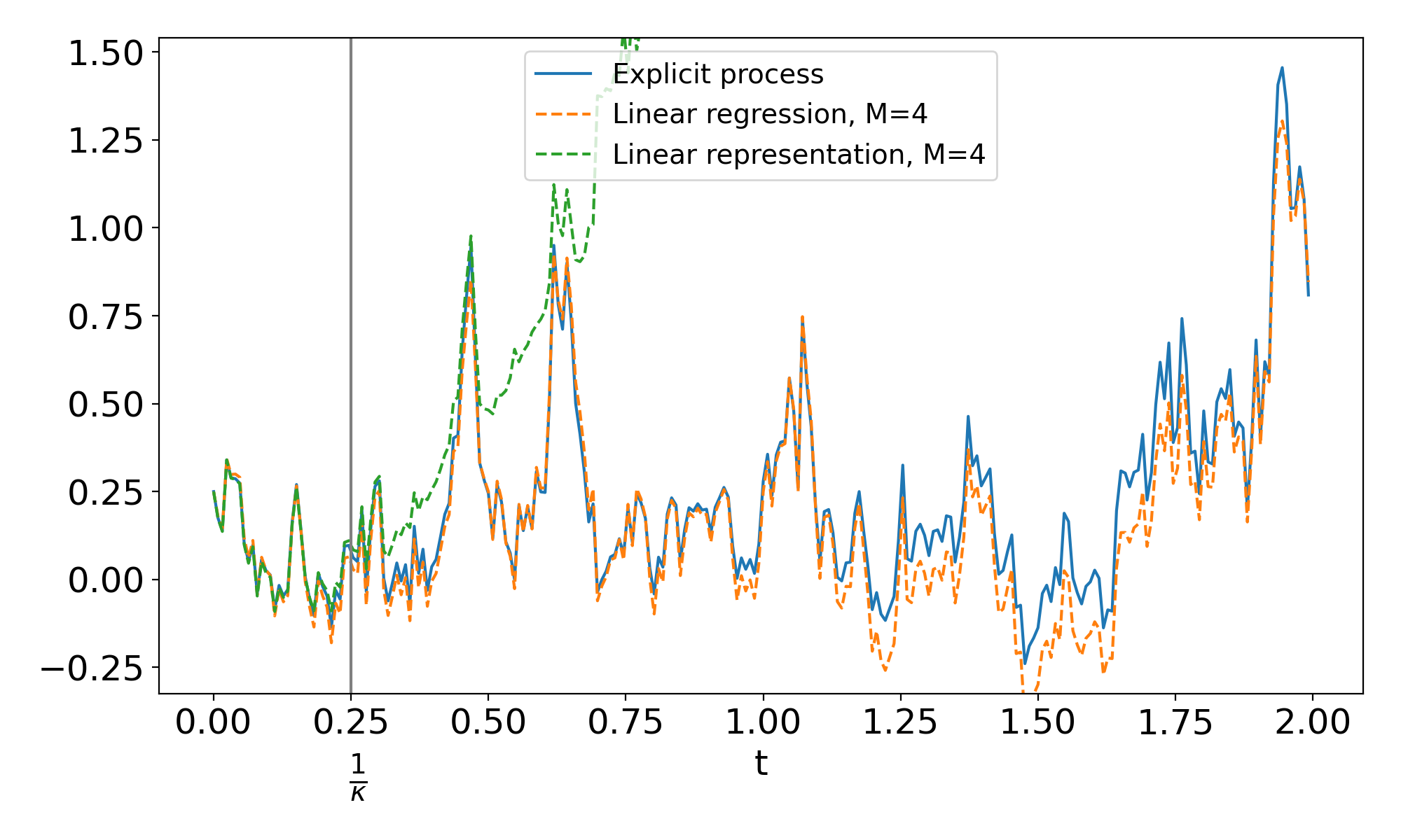
(b) $T=2$.

Figure 10: Trajectories of a mean-reverting geometric Brownian motion against their linear representation and linear regression. $\kappa=4,\theta=0.25,\eta=1,\alpha=2$

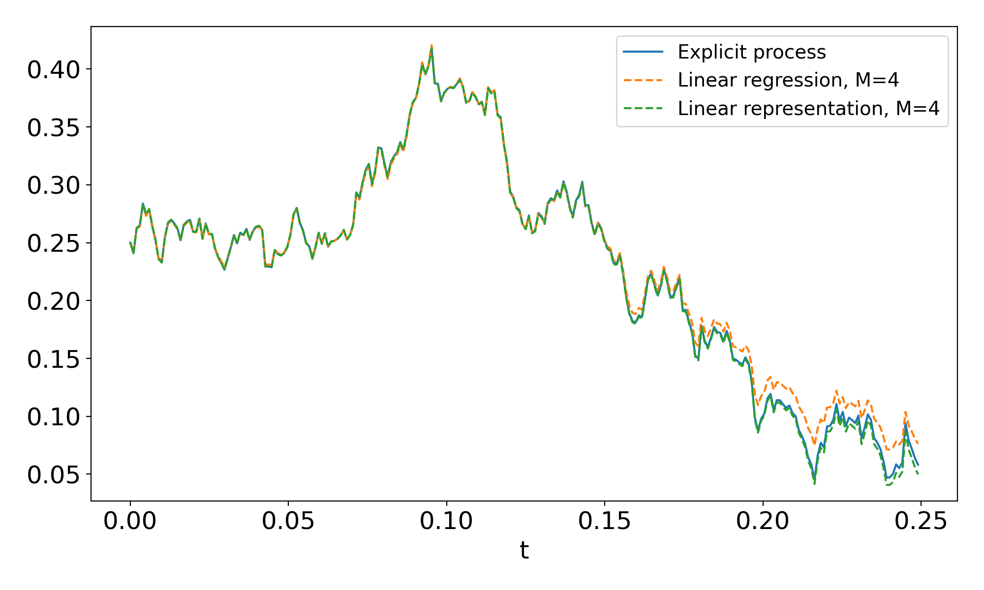
(a) $T=0.25$.

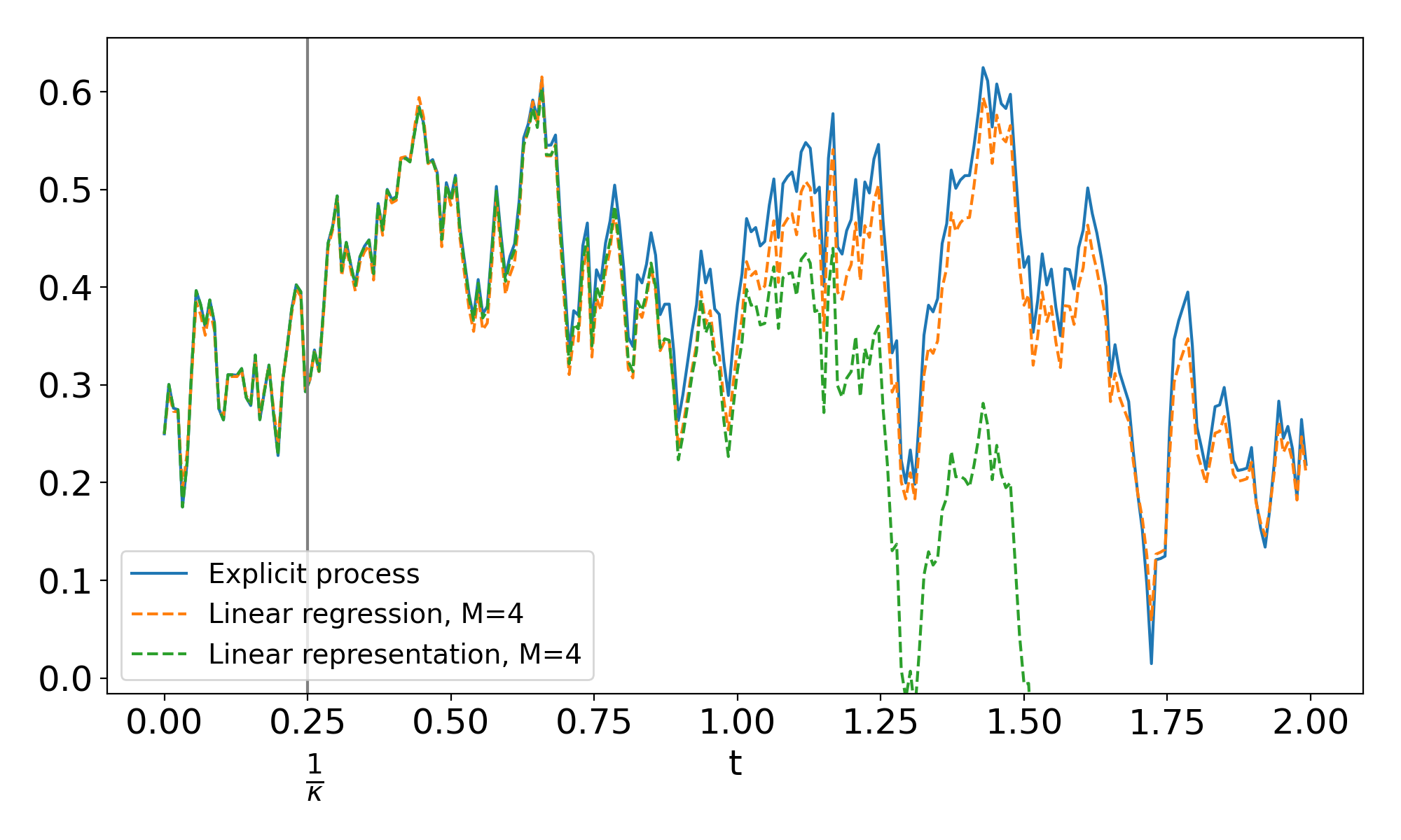
(b) $T=2$.

Figure 11: Trajectories of a square-root Cox-Ingersoll-Ross process against their linear representation and linear regression. $\kappa=4,\theta=0.0625,\eta=1$

However, this stability across the training horizon could easily be interpreted as overfitting. Table 1 below displays the mean squared error between explicit simulations of an Ornstein-Uhlenbeck process and their linear representations (exact truncated and from a regression) where $\kappa=4,\theta=0.25,\eta=2$ and $v=0.25$. The number of simulations and training horizon have been set to 100 000 and 1 year with 252 time steps respectively, see also Figure 12.

MSE		Test horizon
		3 months	6 months	1 year	2 years	4 years
$M=2$	Exact	3.065e-05	5.370e-03	1.969e+00	2.536e+01	2.625e+02
	Regression	6.149e-03	8.564e-03	2.405e-02	6.239e-01	1.189e+01
$M=4$	Exact	6.541e-08	1.736e-05	1.718e+00	4.243e+02	8.177e+04
	Regression	8.002e-06	3.801e-05	1.079e-04	1.516e+00	1.213e+03
$M=6$	Exact	5.908e-08	1.167e-06	3.173e-01	1.410e+03	4.872e+06
	Regression	5.735e-06	8.426e-06	1.596e-07	1.066e+00	3.188e+04

Table 1: Mean-squared-error between simulations of an Ornstein-Uhlenbeck process against its linear representation and linear regression when trained over only 1 year. $\kappa=4,\theta=0.25,\eta=2$.

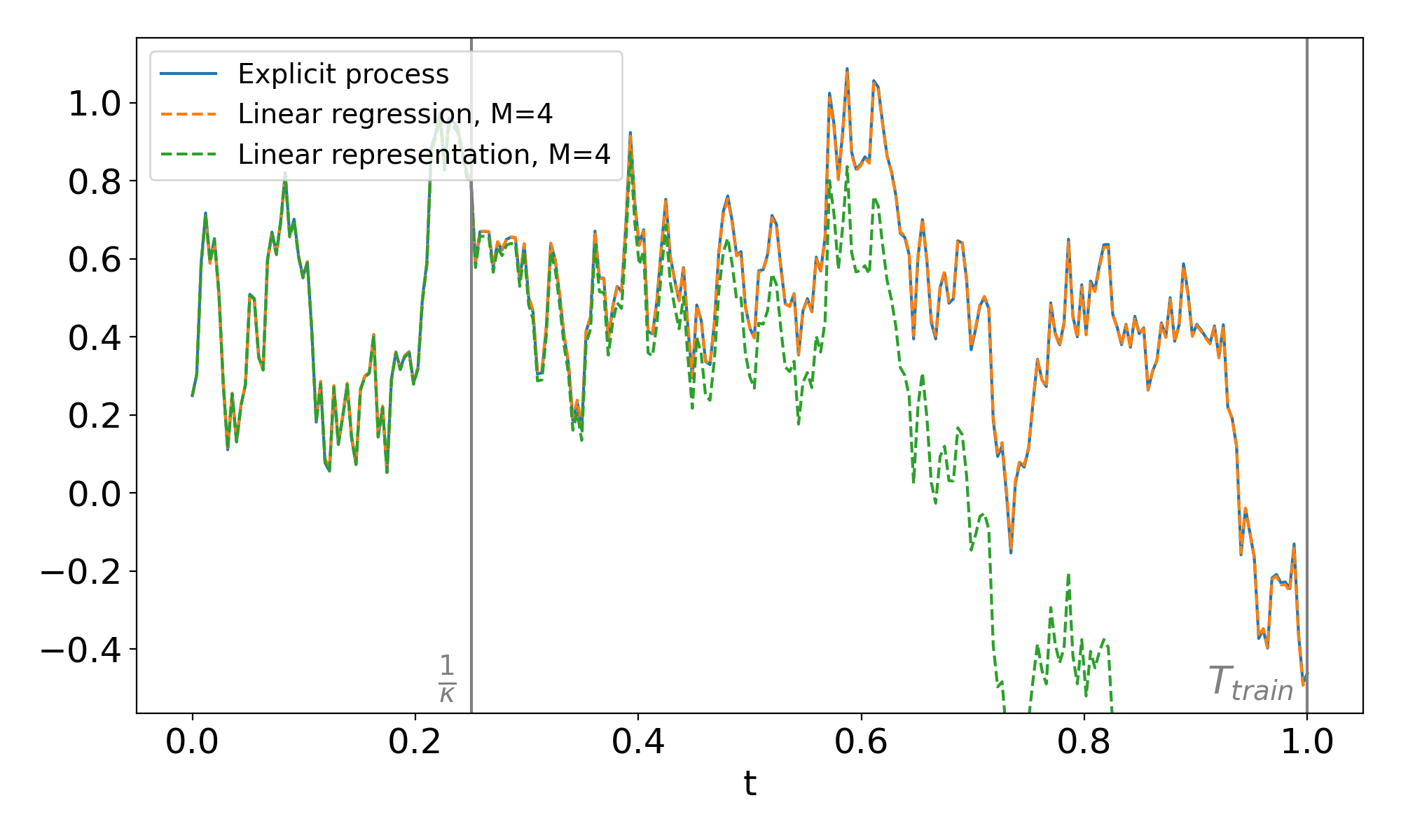
(a) $T=1$.

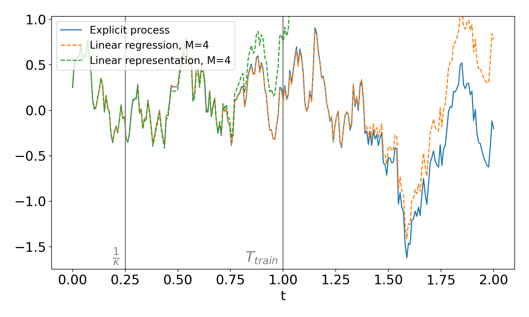
(b) $T=2$.

Figure 12: Trajectories of an Ornstein-Uhlenbeck process against their linear representation and linear regression when trained over only 1 year. $\kappa=4,\theta=0.25,\eta=2$.

4 The joint characteristic functional

The following theorem provides the joint conditional characteristic functional of the log-price $\log S$ and the integrated variance $\bar{V}:=\int_{0}^{\cdot}\Sigma^{2}_{s}ds$ in the model (3.2)–(3.3) in terms of a solution to an infinite-dimensional system of time-dependent $T((\mathbb{R}^{2}))$-valued Riccati differential equations.

Theorem 4.1.

Let $f,g:[0,T]\to\mathbb{C}$ be measurable and bounded functions and $\bm{\sigma}:[0,T]\to\mathcal{A}$. Assume that there exists $\bm{\psi}\in\mathcal{I}^{\prime}$, solution to the following infinite-dimensional system of time-dependent Riccati equations

$$-\dot{\bm{\psi}}_{t} =\frac{1}{2}(\bm{\psi}_{t}|_{{\mathcolor{NavyBlue}{\mathbf{2}}}})^{\mathrel{\sqcup\mkern-3.2mu\sqcup}2}+\rho f(t)(\bm{\sigma}_{t}\mathrel{\sqcup\mkern-3.2mu\sqcup}\bm{\psi}_{t}|_{{\mathcolor{NavyBlue}{\mathbf{2}}}})+\frac{1}{2}\bm{\psi}_{t}|_{{\mathcolor{NavyBlue}{\mathbf{22}}}}+\bm{\psi}_{t}|_{{\mathcolor{NavyBlue}{\mathbf{1}}}}+\left(\frac{f(t)^{2}-f(t)}{2}+g(t)\right)\bm{\sigma}_{t}^{\mathrel{\sqcup\mkern-3.2mu\sqcup}2},$$ (4.1)

$$\bm{\psi}_{T} =0.$$ (4.2)

Define the processes

$$U_{t} =\left\langle\bm{\psi}_{t},\widehat{\mathbb{W}}_{t}\right\rangle+\int_{0}^{t}f(s)d\log S_{s}+\int_{0}^{t}g(s)d\bar{V}_{s},$$ (4.3)

and

$$M_{t} =e^{U_{t}}.$$ (4.4)

Then $M$ is a local martingale. If in addition it is a true martingale, then the following expression holds for the joint characteristic functional of $(\log S,\bar{V})$:

$$\mathbb{E}\left[\left.\exp\left(\int_{t}^{T}f(s)d\log S_{s}+\int_{t}^{T}g(s)d\bar{V}_{s}\right)\right|\mathcal{F}_{t}\right]=\exp\left(\left\langle\bm{\psi}_{t},\widehat{\mathbb{W}}_{t}\right\rangle\right),\quad t\leq T.$$ (4.5)

Proof.

To show that $M$ is a local martingale we show that its part in $dt$ vanishes using Itô’s formula. The dynamics of $M$ read

$$dM_{t}=M_{t}\left(dU_{t}+\frac{1}{2}d\left[U\right]_{t}\right).$$ (4.6)

We start by deriving the dynamics of $U$ in (4.3). By using Lemma 2.7, since $\bm{\psi}\in\mathcal{I}^{\prime}$ by assumption, we have that $\left(\left\langle\bm{\psi}_{t},\widehat{\mathbb{W}}_{t}\right\rangle\right)_{t\geq 0}$ is a semimartingale with dynamics

$$d\left\langle\bm{\psi}_{t},\widehat{\mathbb{W}}_{t}\right\rangle =\left\langle\dot{\bm{\psi}}_{t}+\bm{\psi}_{t}|_{{\mathcolor{NavyBlue}{\mathbf{1}}}}+\tfrac{1}{2}\bm{\psi}_{t}|_{{\mathcolor{NavyBlue}{\mathbf{22}}}},\widehat{\mathbb{W}}_{t}\right\rangle dt+\left\langle\bm{\psi}_{t}|_{{\mathcolor{NavyBlue}{\mathbf{2}}}},\widehat{\mathbb{W}}_{t}\right\rangle dW_{t}.$$

Combining the previous identity with $d\bar{V}_{t}=\langle\bm{\sigma}_{t}^{\mathrel{\sqcup\mkern-3.2mu\sqcup}2},\widehat{\mathbb{W}}_{t}\rangle dt$, recall (3.5), and the dynamics of $\log S$ in (3.22), we obtain that

$$dU_{t} =d\left\langle\bm{\psi}_{t},\widehat{\mathbb{W}}_{t}\right\rangle+f(t)d\log S_{t}+g(t)d\bar{V}_{t}$$

$$=\left\langle\dot{\bm{\psi}}_{t}+\bm{\psi}_{t}|_{{\mathcolor{NavyBlue}{\mathbf{1}}}}+\tfrac{1}{2}\bm{\psi}_{t}|_{{\mathcolor{NavyBlue}{\mathbf{22}}}},\widehat{\mathbb{W}}_{t}\right\rangle dt+\left\langle\bm{\psi}_{t}|_{{\mathcolor{NavyBlue}{\mathbf{2}}}},\widehat{\mathbb{W}}_{t}\right\rangle dW_{t}$$

$$\qquad+\left(g(t)-\tfrac{1}{2}f(t)\right)\left\langle\bm{\sigma}_{t}^{\mathrel{\sqcup\mkern-3.2mu\sqcup}2},\widehat{\mathbb{W}}_{t}\right\rangle dt+f(t)\left\langle\bm{\sigma}_{t},\widehat{\mathbb{W}}_{t}\right\rangle dB_{t}$$

$$=\left\langle\dot{\bm{\psi}}_{t}+\bm{\psi}_{t}|_{{\mathcolor{NavyBlue}{\mathbf{1}}}}+\tfrac{1}{2}\bm{\psi}_{t}|_{{\mathcolor{NavyBlue}{\mathbf{22}}}}+\left(g(t)-\tfrac{1}{2}f(t)\right)\bm{\sigma}_{t}^{\mathrel{\sqcup\mkern-3.2mu\sqcup}2},\widehat{\mathbb{W}}_{t}\right\rangle dt$$

$$\qquad+\left\langle\bm{\psi}_{t}|_{{\mathcolor{NavyBlue}{\mathbf{2}}}},\widehat{\mathbb{W}}_{t}\right\rangle dW_{t}+f(t)\left\langle\bm{\sigma}_{t},\widehat{\mathbb{W}}_{t}\right\rangle dB_{t}.$$

Using the shuffle product of Proposition 2.6 and the fact that $B$ and $W$ are correlated, recall (3.1), we get that the quadratic variation of $U$ is

$$d\left[U\right]_{t} =\left\langle(\bm{\psi}_{t}|_{{\mathcolor{NavyBlue}{\mathbf{2}}}})^{\mathrel{\sqcup\mkern-3.2mu\sqcup}2}+2\rho f(t)(\bm{\psi}_{t}|_{{\mathcolor{NavyBlue}{\mathbf{2}}}}\mathrel{\sqcup\mkern-3.2mu\sqcup}\bm{\sigma}_{t})+f(t)^{2}\bm{\sigma}_{t}^{\mathrel{\sqcup\mkern-3.2mu\sqcup}2},\widehat{\mathbb{W}}_{t}\right\rangle dt.$$

This yields that the drift of $dM_{t}/M_{t}$ in (4.6) is given by

$$\left\langle\dot{\bm{\psi}}_{t}+\bm{\psi}_{t}|_{{\mathcolor{NavyBlue}{\mathbf{1}}}}+\tfrac{1}{2}\bm{\psi}_{t}|_{{\mathcolor{NavyBlue}{\mathbf{22}}}}+\left(g(t)-\tfrac{1}{2}f(t)\right)\bm{\sigma}_{t}^{\mathrel{\sqcup\mkern-3.2mu\sqcup}2}\right.$$

$$\qquad\left.+\tfrac{1}{2}\left[(\bm{\psi}_{t}|_{{\mathcolor{NavyBlue}{\mathbf{2}}}})^{\mathrel{\sqcup\mkern-3.2mu\sqcup}2}+2\rho f(t)(\bm{\psi}_{t}|_{{\mathcolor{NavyBlue}{\mathbf{2}}}}\mathrel{\sqcup\mkern-3.2mu\sqcup}\bm{\sigma}_{t})+f(t)^{2}\bm{\sigma}_{t}^{\mathrel{\sqcup\mkern-3.2mu\sqcup}2}\right],\widehat{\mathbb{W}}_{t}\right\rangle,$$

which is equal to $0$ from the Riccati equations (4.1). This shows that $M$ is a local martingale. By assumption $M$ is even a true martingale. After observing that the terminal value of $M$, is given by

$$M_{T}=\exp\left(\int_{0}^{T}f(s)d\log S_{s}+\int_{0}^{T}g(s)d\bar{V}_{s}\right),$$

recall that $\bm{\psi}_{T}=0$, we obtain

$$\mathbb{E}\left[\exp\left(\int_{0}^{T}f(s)d\log S_{s}+\int_{0}^{T}g(s)d\bar{V}_{s}\right)\bigg{|}\mathcal{F}_{t}\right]=\mathbb{E}\left[M_{T}\big{|}\mathcal{F}_{t}\right]=M_{t}=\exp\left(U_{t}\right),$$

which yields (4.5). ∎

Theorem 4.1 is a verification result to obtain the exponentially affine representation of the joint characteristic functional (4.5). It disentangles the algebraic affine structure in infinite dimension. It can be related to [29, Theorem 4.24] if one considers the signature of the three dimensional process $((t,W_{t},B_{t}))_{t\geq 0}$ there. It relies on the two crucial assumptions that a well-behaved $\mathcal{I}$-valued solution $\bm{\psi}$ exists to the Riccati equation (4.1), together with the true martingality of $M$. These assumptions seem very intricate to prove, even in one dimensional settings, partial results in these directions for $T((\mathbb{R}))$-valued Riccati equations can be found in [29, Section 6] and [7]. We note that no semimartingality assumption for $\Sigma_{t}=\langle\bm{\sigma}_{t},\widehat{\mathbb{W}}_{t},\rangle$ is required in Theorem 4.1.

In the following two sections, we will validate the representation (4.5) numerically and we will highlight the application of Theorem 4.1 to the pricing and the hedging of several contingent claims by Fourier inversion techniques. The general functions $f$ and $g$ allow for enough flexibility to cover a broad set of contingent claims. For instance:

1. Certain vanilla options that depend on the values $(S_{T},\bar{V}_{T})$, like European call and put options and volatility swaps, are recovered using constant $f$ and $g$.

2. Geometric Asian options on the average $\frac{1}{T}\int_{0}^{T}\log S_{s}ds$ can be recovered by setting $f(s):=iu\frac{T-s}{T}$, since

   $$\int_{t}^{T}f(s)d\log S_{s} =iu\int_{t}^{T}\frac{T-s}{T}d\log S_{s}$$ (4.7)

   $$=iu\frac{1}{T}\int_{t}^{T}\log S_{s}ds-iu\frac{T-t}{T}\log S_{t}.$$ (4.8)

5 Pricing by Fourier methods

In this section, we show how Theorem 4.1 can be applied to price European and Asian call and put options as well as $q$-Volatility swaps using Fourier inversion techniques in our signature volatility model (3.2)-(3.3). All of our numerical results validate the exponentially affine representation (4.5). We also provide a calibration to market volatility surface for the S&P 500.

For the numerical implementation, we consider a truncated version of $S$ from (3.2)-(3.3), denoted by $S^{\leq M}$ and defined by

$$dS_{t}^{\leq M}=S_{t}^{\leq M}\left\langle\bm{\sigma}_{t}^{\leq M},\widehat{\mathbb{W}}_{t}\right\rangle dB_{t},$$

where $\bm{\sigma}_{t}^{\leq M}\in T^{M}(\mathbb{R}^{2})$ has its first $M$ levels coincide with $\bm{\sigma}_{t}$ and is $0$ elsewhere. Finally, in order to ease notations in the sequel we assume $S_{0}=1$ (recall that the short rate here is assumed to be $0$).

5.1 European options

Let us consider a European call option on $S$ with maturity $T>0$ and strike $K>0$. Its price at time $t\leq T$ is given by $C_{t}(T,K)=\mathbb{E}[(S_{T}-K)^{+}|\mathcal{F}_{t}]$. From Lewis [45], one can price this option using the Fourier inversion formula

$$C_{t}(S_{t};T,K)=S_{t}-\frac{K}{\pi}\int_{0}^{\infty}\,\mathfrak{Re}\left[e^{i(u-\frac{i}{2})k_{t}}\phi_{t}\left(u-\tfrac{i}{2}\right)\right]\frac{du}{\left(u^{2}+\tfrac{1}{4}\right)},$$ (5.1)

where $\phi$ is the conditional characteristic function $\phi_{t}(u)=\mathbb{E}\left[e^{iu\log\frac{S_{T}}{S_{t}}}|\mathcal{F}_{t}\right]$ and $k_{t}=\log\frac{S_{t}}{K}$.

Moreover, we add a ‘control variate’ to quicken the convergence, as in Andersen and Andreasen [8]. Given $\sigma_{\textnormal{BS}}<\infty$, one has

$$C_{t}(S_{t};T,K)=C_{t}^{\textnormal{BS}}(S_{t};T,K)-\frac{K}{\pi}\int_{0}^{\infty}\,\mathfrak{Re}\left[e^{i(u-\frac{i}{2})k_{t}}\left(\phi_{t}\left(u-\tfrac{i}{2}\right)-\phi_{t}^{\textnormal{BS}}\left(u-\tfrac{i}{2}\right)\right)\right]\frac{du}{\left(u^{2}+\tfrac{1}{4}\right)},$$ (5.2)

where

$$C_{t}^{\textnormal{BS}}(S_{t};K,T) =\mathcal{N}(d_{1})S_{t}-\mathcal{N}(d_{2})K,$$ (5.3)

with

$$d_{1}=\frac{1}{\sigma_{\textnormal{BS}}\sqrt{T-t}}\left(\log\frac{S_{t}}{K}+\frac{\sigma_{\textnormal{BS}}^{2}}{2}(T-t)\right),\quad d_{2}=d_{1}-\sigma_{\textnormal{BS}}\sqrt{T-t}$$ (5.4)

and

$$\phi_{t}^{\textnormal{BS}}(u) =\exp\left[-\frac{\sigma_{\textnormal{BS}}^{2}}{2}\left(u^{2}+iu\right)(T-t)\right].$$ (5.5)

This Black-Scholes control variate can also be applied to other products and, as will be seen in Section 6, to Fourier hedging. The quantity $\sigma_{\textnormal{BS}}$ can be determined to ensure approximate moment matching for instance, and one can use the characteristic function $\phi_{t}$ to approximate (by finite differences) the second order cumulant of the distribution of the log price $\log S$.

Numerically, for the discretization of the Fourier integral, our numerical experiments show that Gauss-Laguerre quadrature outperform other quadrature rules in our class of models, which is in line with the empirical findings that appeared in [54]. In particular, the higher the maturity is, the lower the degree of the quadrature needs to be for the same set of parameters. In addition, the use of a control variate makes computations much quicker yielding fewer calls of the characteristic function to make the quadrature converge, see Figure 13. Moreover, we can see that the added value of the control variate, in terms of speed of convergence, grows with the time horizon. See [54, Section 6] for more details on numerical refinements.

For a given signature volatility model (3.2)-(3.3), i.e. a set of parameters $\bm{\sigma}:[0,T]\to\mathcal{A}$, an application of Theorem 4.1 with $f(t)=iu$ and $g=0$ provides the characteristic function $\phi_{t}(u)$ modulo the solution $\bm{\psi}$ to the $T((\mathbb{R}^{2}))$-valued Riccati equation (4.1), which allows us to compute the price of call options in the signature volatility model using (5.2) together with a suitable truncation and discretization of the Riccati equation (4.1). The truncation rule for $\bm{\psi}$ is not trivial and requires a little bit of care, because the shuffle products cannot be exact, as each step of the discretized ODE would double the truncation order of $\bm{\psi}$. For the numerical implementation, we decided to fix the order $\tilde{M}$ of $\bm{\psi}$ for each step and hence only have a shuffle product projected on $T^{\tilde{M}}(\mathbb{R}^{2})$, i.e. $\widetilde{\mathrel{\sqcup\mkern-3.2mu\sqcup}}:(T^{\tilde{M}}(\mathbb{R}^{2}))^{2}\to T^{\tilde{M}}(\mathbb{R}^{2})$. Obviously, choosing $\tilde{M}$ lower than $2M$, where $M$ is the truncation order of $\bm{\sigma}$, also induces an approximation of shuffle product in $\bm{\sigma}^{\mathrel{\sqcup\mkern-3.2mu\sqcup}2}$, which greatly deteriorated the quality of the convergence, if not prevented it altogether. We thus fixed $\tilde{M}=2M$ throughout our experiments. Said differently for a given signature volatility $\bm{\sigma}\in T^{M}(\mathbb{R}^{2})$ the truncated solution $\bm{\psi}$ to the Riccati equation (4.1) is an element of $T^{2M}(\mathbb{R}^{2})$. Regarding the numerical discretization and in order for the Riccati to converge in a realistic amount of time, we use Runge-Kutta to the 4th order to solve the ODE, which computes 4 times as many points as the Euler direct algorithm, but converges more than 4 times as fast. We also compute the characteristic function both JIT and in parallel so that it is drastically faster.

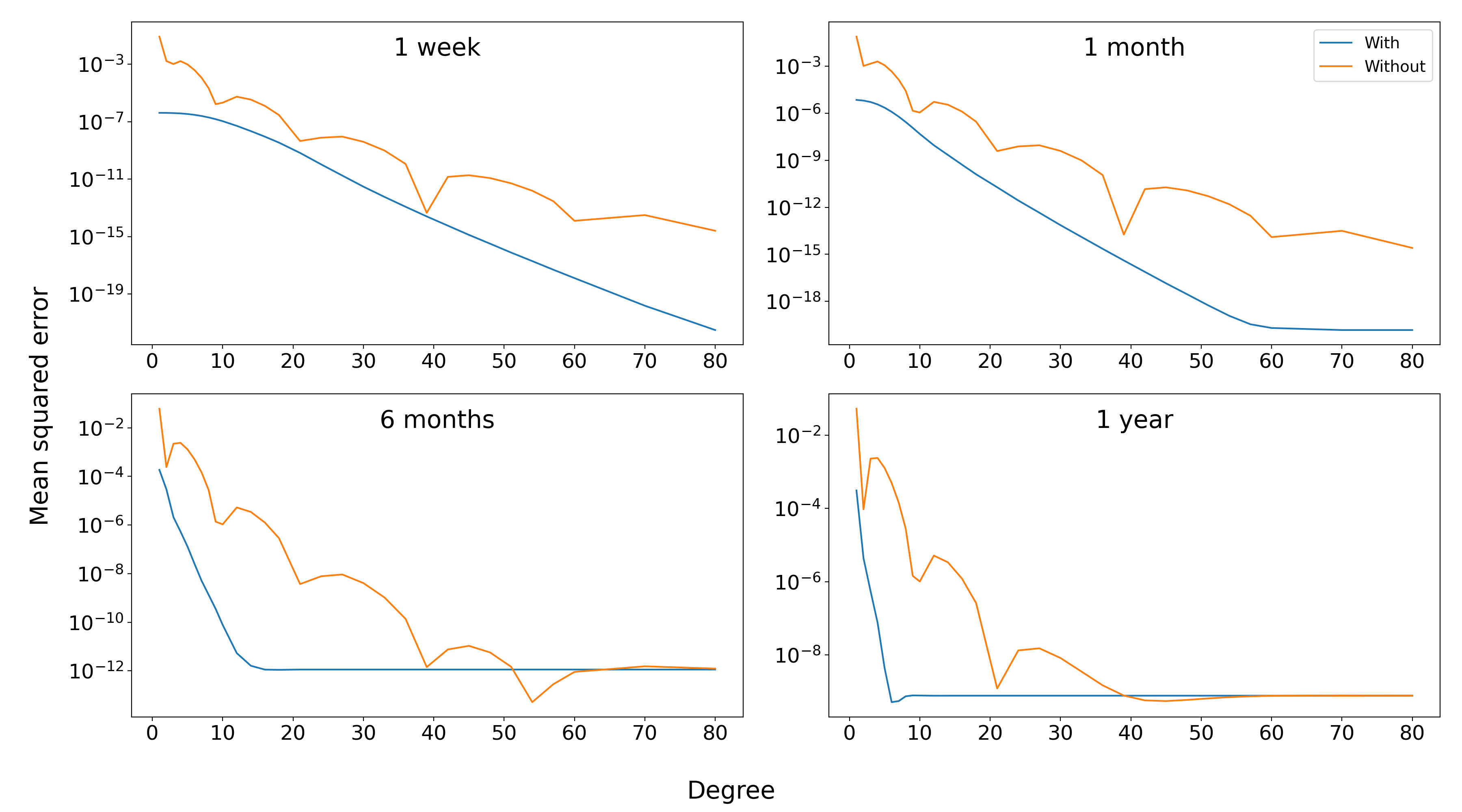
Figure 13: Gauss-Laguerre quadrature mean-squared-error of put pricing with and without control variate, under Stein-Stein model. $\kappa=1,\theta=0.25,\eta=1.2$ and $\rho=-0.5$.

In Figures 14 and 15, we compare our Signature volatility pricing using the linear representations of the Ornstein-Uhlenbeck (3.8) and Cox-Ingersoll-Ross (3.18) representations, truncated at order $M=4$, to the explicit Fourier pricing of the Stein-Stein [58] and Heston [42] models. Lewis’ approach together with Black-Scholes control variate, see (5.2), was used. This serves as a numerical validation for Theorem 4.1 as well as for our conjectured representation for the square-root process (3.18).

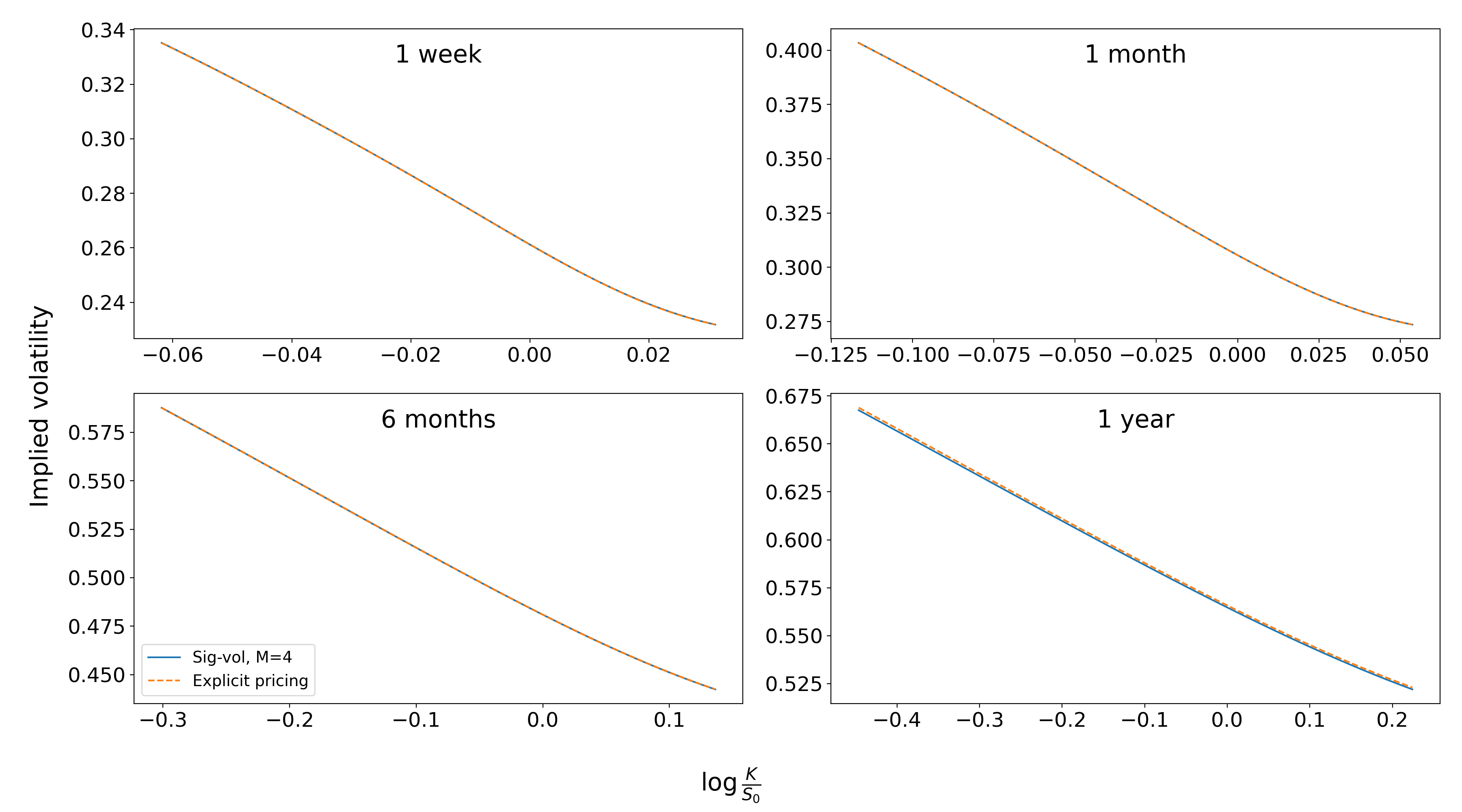
Figure 14: European call Fourier pricing of Stein-Stein model vs Signature Ornstein-Uhlenbeck volatility model (3.8). $\kappa=1,\theta=0.25,\eta=1.2$ and $\rho=-0.5$.

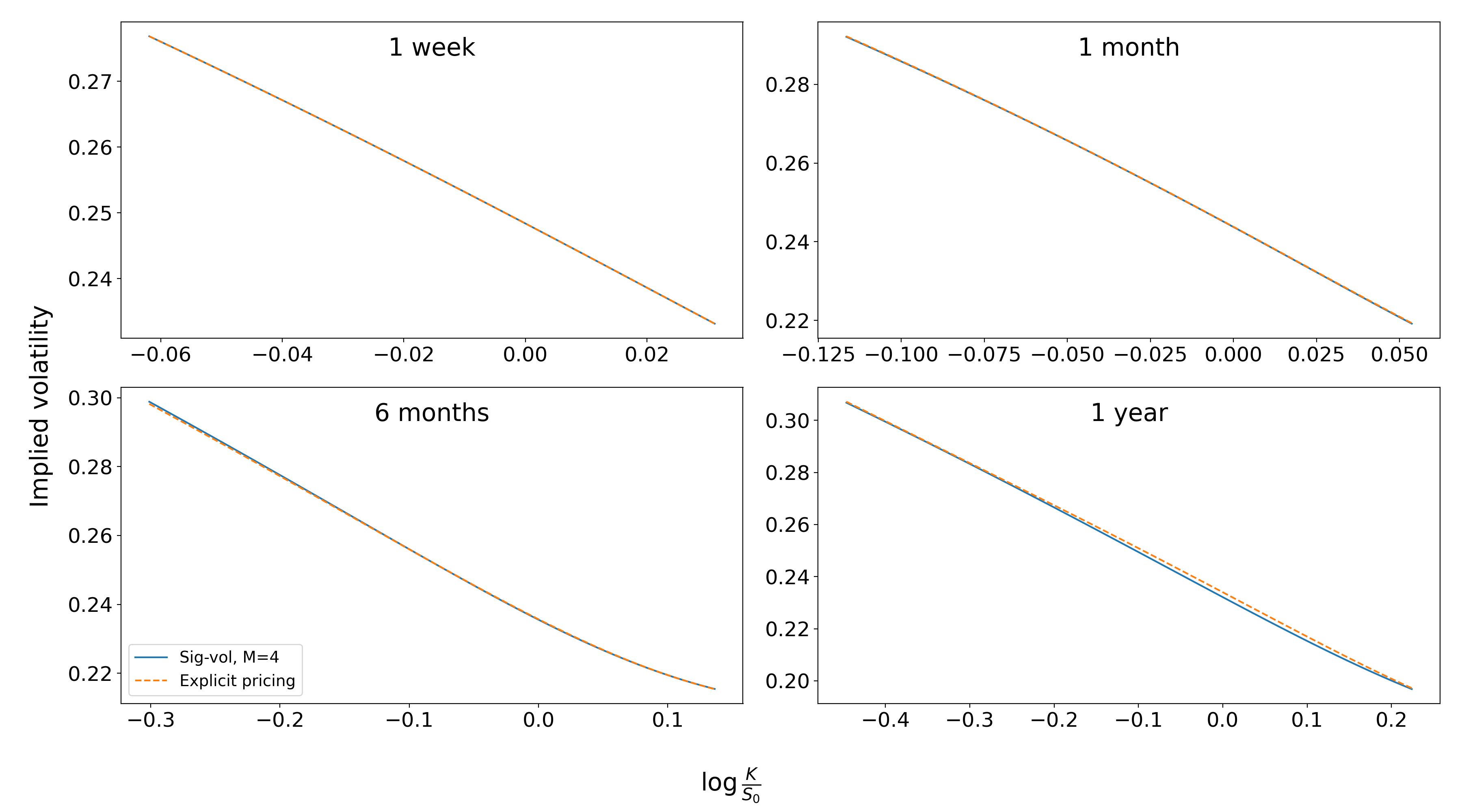
Figure 15: European call Fourier pricing of Heston model vs Signature square-root Cox-Ingersoll-Ross volatility model (3.18). $\kappa=4,\theta=0.0625,\eta=0.7$ and $\rho=-0.7$.

In Figure 16 we compare our signature volatility pricing using the linear mean-reverting geometric Brownian motion representation (3.12) truncated at order $M=4$ to Monte Carlo simulations, see Remark 3.14. Lewis’ approach together with Black-Scholes control variate was also used.

Figure 16: European call Monte Carlo pricing of mGBM volatility model vs Fourier pricing of Signature mean-reverting geometric Brownian motion volatility model (3.12). $\kappa=1,\theta=0.25,\eta=1.2,\alpha=0.6$ and $\rho=-0.5711$.

In Figure 17 we work on a linear functional drawn at random under the leverage effect condition (LER), see (3.21). In this example, the coefficients $\bm{\sigma}^{\textnormal{LER}}$ are drawn such that

1. $\bm{\sigma}^{\textnormal{LER}{\color[rgb]{0.0600000000000001,0.46,1}\textup{{\o{}}}}}=x$,

2. the coefficients that must remain positive have been drawn from a $\mathcal{U}_{[0,0.5]}$,

3. the unconstrained coefficients have been drawn from a $\mathcal{U}_{[-0.5,0.5]}$.

Bellow is the draw used in Figure 17:

$$\bm{\sigma}^{\textnormal{LER}}=\left(0.25,\begin{pmatrix}-0.0644715\\ 0.36712438\end{pmatrix},\begin{pmatrix}0.05250405&0\\ -0.02796828&0\end{pmatrix},\begin{pmatrix}-0.3698671&0&\\ 0.05678161&0&\\ &0.3307244&0\\ &0.2119773&0.2379793\end{pmatrix},\bm{0}\right).$$ (5.6)

Then, using $\bm{\sigma}^{\textnormal{LER}}$, we compute Monte Carlo simulations, i.e. we simulate Brownian motions, augment them with time and compute their signature. We then compute the linear combination of $\bm{\sigma}^{\textnormal{LER}}$ against each simulated signature. This further validates Theorem 4.5 and highlights the efficiency of our numerical implementation using Gauss-Laguerre quadrature, a Black-Scholes control variate and the fourth-order Runge-Kutta scheme for the truncated tensor algebra valued Riccati equation.

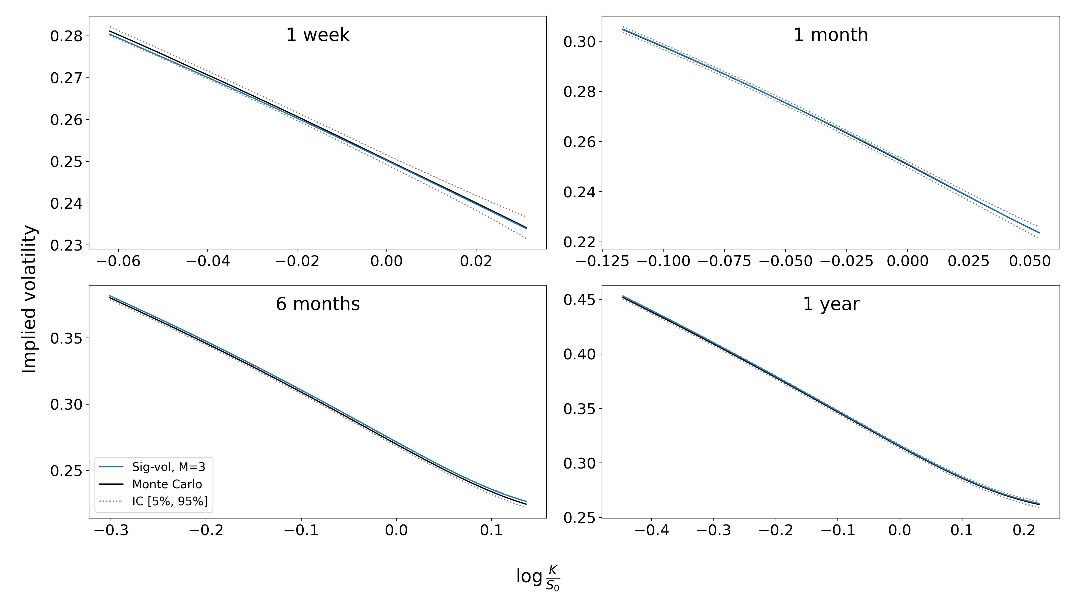
Figure 17: European put Monte Carlo pricing of LER linear volatility model vs Fourier pricing of Signature LER volatility model. $\bm{\sigma}^{\textnormal{LER}}$ defined in (5.6).

5.2 Asian options

Let us consider a geometric Asian call option with price $\bar{C}_{t}(T,K)=\mathbb{E}[(\bar{S}_{T}-K)^{+}|\mathcal{F}_{t}]$, where $\bar{S}_{t}=\exp\left(\frac{1}{T}\int_{0}^{t}\log S_{s}ds\right)$. Similarly to (5.2), we obtain the Fourier representation

$$\bar{C}_{t}(\bar{S}_{t};T,K)=\bar{C}_{t}^{\textnormal{BS}}(\bar{S}_{t};T,K)-\frac{K}{\pi}\int_{0}^{\infty}\,\mathfrak{Re}\left[e^{i(u-\frac{i}{2})\bar{k}_{t}}\left(\bar{\phi}_{t}\left(u-\tfrac{i}{2}\right)-\bar{\phi}_{t}^{\textnormal{BS}}\left(u-\tfrac{i}{2}\right)\right)\right]\frac{du}{\left(u^{2}+\tfrac{1}{4}\right)},$$ (5.7)

where $\bar{\phi}$ is the characteristic function $\bar{\phi}_{t}(u)=\mathbb{E}\Big{[}e^{iu\log\frac{\bar{S}_{T}}{\bar{S}_{t}}}\Big{|}\mathcal{F}_{t}\Big{]}$ and $\bar{k}_{t}=\log\frac{\bar{S}_{t}}{K}$ with

$$\bar{\phi}_{t}^{\textnormal{BS}}=\exp\left(-\frac{\sigma_{\textnormal{BS}}^{2}}{2}\left(u^{2}\frac{(T-t)^{3}}{3T^{2}}+iu\frac{(T-t)^{2}}{2T}\right)\right),$$ (5.8)

and where

$$\bar{C}_{t}^{\textnormal{BS}}(\bar{S}_{t};T,K):=\mathcal{N}(\bar{d}_{1})\bar{S}_{t}\exp\left(\frac{T-t}{T}\log S_{t}-\frac{\sigma^{2}_{\textnormal{BS}}}{2}\left(\frac{(T-t)^{2}}{2T}-\frac{(T-t)^{3}}{3T^{2}}\right)\right)+\mathcal{N}(\bar{d}_{2})K,$$ (5.9)

and

$$\bar{d}_{2}:=\frac{1}{\sigma_{\textnormal{BS}}\sqrt{\frac{(T-t)^{3}}{3T^{2}}}}\left(\log\frac{\bar{S}_{t}}{K}+\frac{T-t}{T}\log S_{t}-\frac{\sigma^{2}_{\textnormal{BS}}}{2}\frac{(T-t)^{2}}{2T}\right),\quad\bar{d}_{1}:=\bar{d}_{2}-\sigma_{\textnormal{BS}}\sqrt{\frac{(T-t)^{3}}{3T^{2}}}.$$ (5.10)

In Figure 18, we compare our signature volatility Fourier pricing for Asian options using the truncated, at order $M=4$, representation of the linear Ornstein-Uhlenbeck (3.8) to Monte Carlo simulations. Lewis’ approach together with Black-Scholes control variate was also used.

Figure 18: Asian put Monte Carlo pricing of Stein-Stein model vs Signature Ornstein-Uhlenbeck volatility model. $\kappa=1,\theta=0.25,\eta=1.2$ and $\rho=-0.9$.

5.3 q-Volatility swaps

The payoff of a $q$-volatility swap is $R_{T}^{q}-K^{q}$ where $R_{T}^{q}=\left(\frac{1}{T}\bar{V}_{T}\right)^{q}$ is the realized $q$-volatility and $K^{q}$ the $q$-volatility strike. The aim in pricing $q$-volatility swaps is to find the fair strike price, i.e. $K^{q}=\mathbb{E}[R_{T}^{q}]$. This is made possible by Laplace inversion:

Theorem 5.1 (Schürger [56]).

Let $X\geq 0$ be a random variable, then

$$\mathbb{E}[X^{q}]=\frac{q}{\Gamma(1-q)}\int_{0}^{\infty}\frac{1-\mathbb{E}\left[e^{-uX}\right]}{u^{q+1}}du,\quad q\in(0,1).$$

It is straightforward to see that setting $f=0$ and $g(t)=-\frac{u}{T}$ in (4.3) gives $\tilde{M}_{0}(u)=\mathbb{E}[e^{-\frac{u}{T}\bar{V}_{T}}]$, which allows us to compute analytically $q$-volatility swaps in the framework of the signature volatility models with

$$\mathbb{E}\left[\left(\frac{1}{T}\bar{V}_{T}\right)^{q}\right]=\frac{q}{\Gamma(1-q)}\int_{0}^{\infty}\frac{1-\tilde{M}_{0}(u)}{u^{q+1}}du.$$

Specifically, the fair strike of the volatility swap, i.e. $q=\frac{1}{2}$, is thus of the form

$$\mathbb{E}\left[\sqrt{\frac{1}{T}\bar{V}_{T}}\right]=\frac{1}{2\sqrt{\pi}}\int_{0}^{\infty}\frac{1-\tilde{M}_{0}(u)}{u^{3/2}}du.$$

Moreover, the fair strike of the variance swap, i.e. $q=1$, can be written in closed form thanks to Fawcett’s formula (3.6) for time-independent representations, i.e.

$$K_{T}^{1}=\frac{1}{T}\left\langle\bm{\sigma}^{\mathrel{\sqcup\mkern-3.2mu\sqcup}2}{\mathcolor{NavyBlue}{\mathbf{1}}},\mathbb{E}[\widehat{\mathbb{W}}_{T}]\right\rangle.$$

(a) $q=\frac{1}{2}$ (volatility swap).

(b) $q=1$ (variance swap).

Figure 19: Strikes of $q$-volatility swaps as a function of the maturity, for a Signature Ornstein-Uhlenbeck volatility model. $\kappa=1,\theta=0.25,\eta=1.2$ and $\rho=-0.7$.

5.4 Calibration examples

Another way to learn the dynamics $\bm{\sigma}$ of the signature volatility is to calibrate it against implied volatility surfaces. In this section, we consider $\bm{\sigma}\in T^{3}(\mathbb{R}^{2})$. We recall that the number of non-zero terms in an object of $T^{M}(\mathbb{R}^{d})$, is $\frac{d^{M+1}-1}{d-1}$. In our case, $d=2$ and we use $M=3$ as it is sufficient to make relatively good fits, i.e. we calibrate 15 parameters. For Figures 20, 21 and 22, we minimized the MSE between a given implied volatility and the one of the signature model, using the differential evolution global minimizer [59].

Figure 20: Implied volatility of time-independent Signature model calibrated against Heston implied volatility surface. $V_{0}=0.25^{2},\kappa=4,\theta=0.0625,\eta=0.7$ and $\rho=-0.6$.

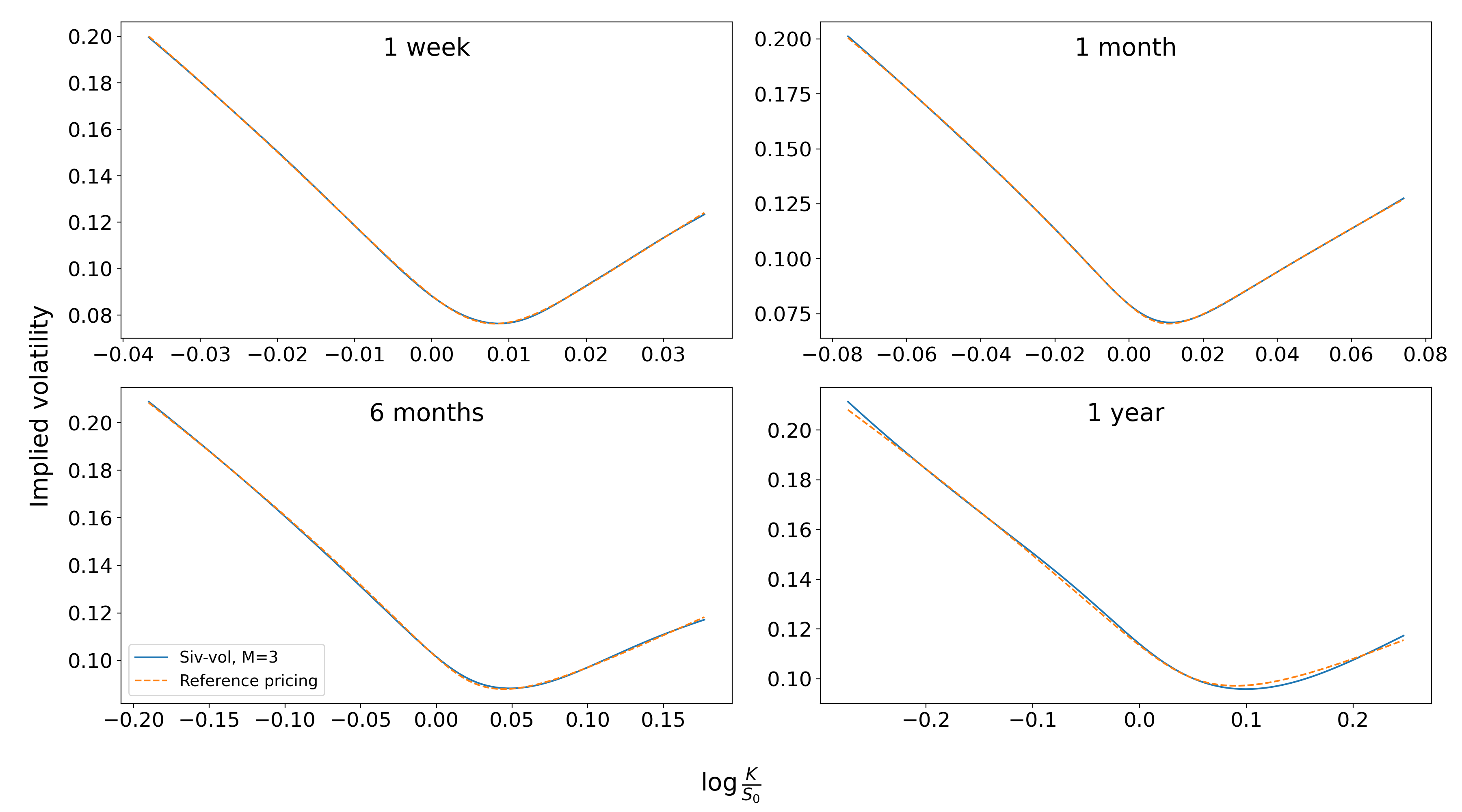
Figure 21: Implied volatility of time-dependent Signature model calibrated against Quintic implied volatility surface. $\xi_{0}(t)\equiv 0.25^{2},H=-0.1,\epsilon=\frac{1}{52},\alpha=\{0.01,1,0,0.214,0,0.227\}$ and $\rho=-0.65$.

Finally, we show how our signature volatility model is well adapted to produce a good fit with daily SPX implied volatility surface data purchased from the CBOE website https://datashop.cboe.com/.

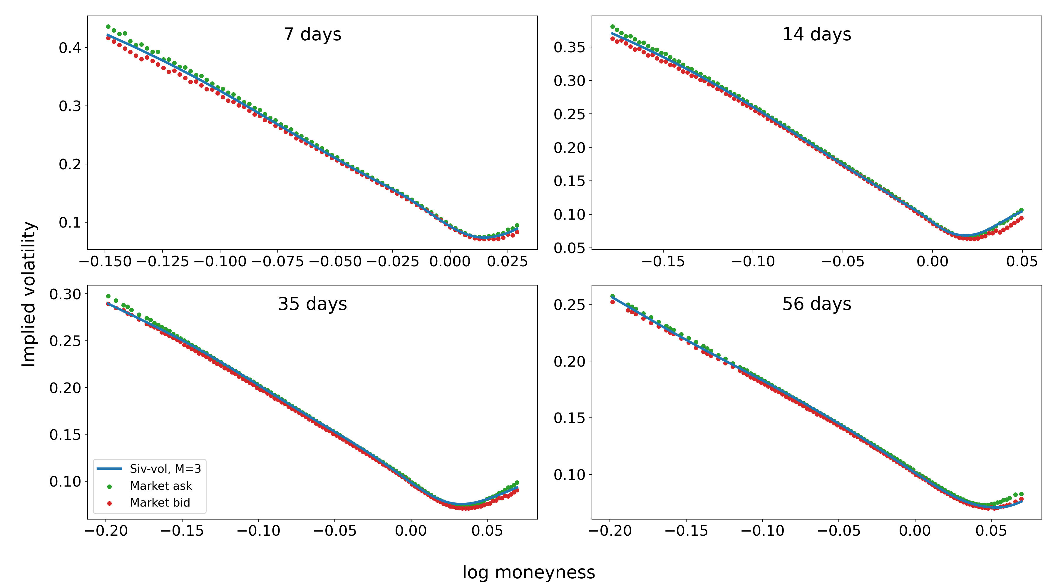
Figure 22: Implied volatility of time-dependent Signature model calibrated against SPX data 2017-05-19.

6 Quadratic hedging by Fourier methods

The signature volatility model (3.2)-(3.3) generates an incomplete market in general (unless the correlation $\rho$ between the two Brownian motions $B$ and $W$ is $\pm 1$). Therefore contingent claims on the stock $S$ cannot be perfectly hedged. We will consider quadratic hedging methods instead, we refer to [57] for a detailed overview of quadratic hedging approaches. We will show that in our setup, quadratic hedging remains highly tractable in signature volatility models using Fourier techniques on the conditional characteristic function (4.5). We do this in two steps:

1. We first solve in Section 6.1 the quadratic hedging problem for a generic contingent claim $\xi$, in a general stochastic volatility model driven by the two dimensional Brownian motion $(W,W^{\perp})$. The hedging strategy depends on the quantities that appear in the martingale representation theorem of $\mathbb{E}[\xi|\mathcal{F}_{t}]$. We provide a concise proof in this setting.

2. We then show in Section 6.2 that in the setting of a signature volatility model and for contingent claims that admit Fourier representation, such as European and Asian call and put options, the hedging strategy can be recovered from the conditional characteristic function (4.5).

6.1 A generic solution

Let $\xi$ be an $\mathcal{F}_{T}$-measurable non-negative random variable such that $\mathbb{E}[\xi^{2}]<\infty$ that we are looking to hedge using a self-financing portfolio. We recall that $(\mathcal{F}_{t})_{t\geq 0}$ is the filtration generated by $(W,W^{\perp})$. A self-financing hedging portfolio $X$ consists of an initial wealth $X_{0}\in\mathbb{R}$ and a progressively measurable strategy $(\vartheta_{u})_{u\leq T}$ of the amount of shares invested in asset $S$ given in (3.2) at time $u\leq T$. It has the following dynamics

$$X_{t}^{\alpha}=X_{0}+\int_{0}^{t}\vartheta_{u}dS_{u}=X_{0}+\int_{0}^{t}\alpha_{u}dB_{u},$$ (6.1)

with $\alpha_{u}:=\vartheta_{u}S_{u}\Sigma_{u}$. The set of admissible hedging strategies $\alpha$ is defined by

$$\mathcal{H}=\left\{\alpha\text{ progressively measurable such that }\int_{0}^{T}\mathbb{E}\left[\alpha_{s}^{2}\right]ds<\infty\right\}.$$ (6.2)

We stress that in this section we do not impose specific dynamics for the stochastic volatility $\Sigma$, i.e. (3.3), $\Sigma$ is only assumed to be adapted to the Brownian motion $(W,W^{\perp})$.

A quadratic hedging strategy aims at minimizing the following objective function

$$J(X_{0},\alpha)=\mathbb{E}\left[\left(X_{T}^{\alpha}-\xi\right)^{2}\right]$$ (6.3)

over $X_{0}\in\mathbb{R}$ and $\alpha\in\mathcal{H}$.

The next theorem provides a solution of the quadratic hedging problem using the martingale representation theorem. Note that $(\mathbb{E}[\xi|\mathcal{F}_{t}])_{t\leq T}$ is a square integrable martingale with terminal value $\xi$ at $T$. An application of the martingale representation theorem [44, Theorem 4.15] yields the existence of two progressively measurable and square integrable processes $Z$ and $Z^{\perp}$ such that

$$\mathbb{E}\left[\xi|\mathcal{F}_{t}\right]=\xi-\int_{t}^{T}Z_{s}dW_{s}-\int_{t}^{T}Z^{\perp}_{s}dW^{\perp}_{s}.$$ (6.4)

Theorem 6.1.

The value of the quadratic hedging problem is given by

$$\inf_{X_{0}\in\mathbb{R},\alpha\in\mathcal{H}}J(X_{0},\alpha)=\mathbb{E}\left[\int_{0}^{T}\left(Z_{t}^{2}+(Z_{t}^{\perp})^{2}\right)dt-\int_{0}^{T}\left(\rho Z_{t}+\sqrt{1-\rho^{2}}Z_{t}^{\perp}\right)^{2}dt\right],$$ (6.5)

where the optimum is attained for $(X_{0}^{*},\alpha^{*})$ given by

$$X_{0}^{*}=\mathbb{E}\left[\xi\right]\quad\text{and}\quad\alpha^{*}_{t}=\rho Z_{t}+\sqrt{1-\rho^{2}}Z_{t}^{\perp},\quad t\leq T.$$ (6.6)

Proof.

We start by expanding the square inside the objective function $J$ in (6.3):

$$(X_{T}^{\alpha}-\xi)^{2}=(X_{T}^{\alpha})^{2}-2\xi X_{T}^{\alpha}+\xi^{2},$$

and we write

$$(X_{T}^{\alpha})^{2} =X_{0}^{2}+2X_{0}\int_{0}^{T}\alpha_{u}dB_{u}+\left(\int_{0}^{T}\alpha_{u}dB_{u}\right)^{2}$$

$$\xi X_{T}^{\alpha} =\mathbb{E}[\xi]X_{0}+\int_{0}^{T}\mathbb{E}[\xi|\mathcal{F}_{s}]dX_{s}^{\alpha}+\int_{0}^{T}X_{s}^{\alpha}d\mathbb{E}[\xi|\mathcal{F}_{s}]+\int_{0}^{T}\alpha_{s}\left(\rho Z_{s}+\sqrt{1-\rho^{2}}Z_{s}^{\perp}\right)ds$$

so that by using the fact that stochastic integrals are centered and by Itô’s isometry we obtain that

$$J(X_{0},\alpha) =\mathbb{E}\left[(X_{0}-\mathbb{E}[\xi])^{2}+\left(\xi^{2}-\mathbb{E}[\xi]^{2}\right)+\int_{0}^{T}\left(\alpha_{s}^{2}-2\alpha_{s}\left(\rho Z_{s}+\sqrt{1-\rho^{2}}Z_{s}^{\perp}\right)\right)ds\right]$$

$$=\mathbb{E}\left[(X_{0}-\mathbb{E}[\xi])^{2}+\int_{0}^{T}\left(Z_{s}^{2}+(Z_{s}^{\perp})^{2}\right)ds+\int_{0}^{T}\left(\alpha_{s}-\alpha_{s}^{*}\right)^{2}ds-\int_{0}^{T}\left(\rho Z_{s}+\sqrt{1-\rho^{2}}Z_{s}^{\perp}\right)^{2}ds\right].$$

It immediately follows that the minimum is clearly attained for $X_{0}^{*}$ and $\alpha^{*}$ given by (6.6) and the claimed expression for the value function (6.5) follows. ∎

6.2 Fourier implementation in the signature volatility model

We now illustrate how the optimal hedging strategy $X_{0}^{*}$ and $\alpha^{*}$ given in (6.6) can be recovered numerically from the knowledge of the conditional characteristic function (4.5) in the specific case of a signature volatility model, i.e. when $\Sigma$ is of the form (3.3) and for contingent claims that admit a Fourier representation.

6.2.1 European call option

In this section, we consider a European call options. In order to implement the quadratic hedging, the idea is to re-express the Fourier inversion formula (5.2) in terms of the process $M_{t}(u)$ in (4.4) with $f(t)=iu$ and $g=0$ and apply Itô. Since in this case

$$M_{t}(u)=\phi_{t}(u)e^{iu\log S_{t}},$$

the representation (5.2) directly leads to

$$C_{t}(S_{t};T,K)=C_{t}^{\textnormal{BS}}(S_{t};T,K)-\frac{K}{\pi}\int_{0}^{\infty}\,\mathfrak{Re}\left[e^{i(u-\frac{i}{2})\log K}\left(M_{t}\left(u-\tfrac{i}{2}\right)-M_{t}^{\textnormal{BS}}\left(u-\tfrac{i}{2}\right)\right)\right]\frac{du}{\left(u^{2}+\tfrac{1}{4}\right)},$$ (6.7)

where

$$M_{t}^{\textnormal{BS}}(u)=\phi_{t}^{\textnormal{BS}}(u)e^{iu\log S_{t}},$$

and $\phi_{t}^{\textnormal{BS}}$ as defined in (5.5). Setting $w(u):=\frac{K}{\pi}\frac{e^{-i(u-\frac{i}{2})\log K}}{u^{2}+\frac{1}{4}}$ and $\tilde{u}:=(u-\frac{i}{2})$, an application of Itô’s formula yields that

$$dC_{t} =dC_{t}^{\textnormal{BS}}+\int_{0}^{\infty}\,\mathfrak{Re}\left[w(u)\left(dM_{t}(\tilde{u})-dM_{t}^{\textnormal{BS}}(\tilde{u})\right)\right]du$$

$$=\Delta_{t}^{\textnormal{BS}}dS_{t}+\left(\Theta_{t}^{\textnormal{BS}}+\tfrac{1}{2}\Gamma_{t}^{\textnormal{BS}}(S_{t}\Sigma_{t})^{2}\right)dt$$

$$\qquad+\int_{0}^{\infty}\,\mathfrak{Re}\Big{[}w(u)\Big{(}M_{t}(\tilde{u})\left(dU_{t}+\tfrac{1}{2}d[U]_{t}\right)$$

$$\qquad\qquad\qquad\qquad\qquad-M_{t}^{\textnormal{BS}}(\tilde{u})\left(d\log M_{t}^{\textnormal{BS}}(\tilde{u})+\tfrac{1}{2}d[\log M^{\textnormal{BS}}(\tilde{u})]_{t}\right)\Big{)}\Big{]}du,$$

where $\Delta_{t}^{\textnormal{BS}}=\frac{\partial}{\partial S_{t}}C_{t}^{\textnormal{BS}}$, $\Theta_{t}^{\textnormal{BS}}=\frac{\partial}{\partial t}C_{t}^{\textnormal{BS}}$ and $\Gamma_{t}^{\textnormal{BS}}=\frac{\partial^{2}}{\partial S_{t}^{2}}C_{t}^{\textnormal{BS}}$. Furthermore, using equalities between Black-Scholes Greeks, one can show that

$$dC_{t} =\Delta_{t}^{\textnormal{BS}}S_{t}\Sigma_{t}dB_{t}+\frac{\Theta_{t}^{\textnormal{BS}}}{\sigma_{\textnormal{BS}}^{2}}\left(\sigma_{\textnormal{BS}}^{2}-\Sigma_{t}^{2}\right)dt$$

$$\qquad+\int_{0}^{\infty}\,\mathfrak{Re}\Big{[}w(u)\Big{(}M_{t}(\tilde{u})\left(\left\langle\bm{\psi}_{t}(\tilde{u})|_{{\mathcolor{NavyBlue}{\mathbf{2}}}},\widehat{\mathbb{W}}_{t}\right\rangle dW_{t}+i\tilde{u}\Sigma_{t}dB_{t}\right)$$

$$\qquad\qquad\qquad\qquad\qquad-M_{t}^{\textnormal{BS}}(\tilde{u})\left[\tfrac{1}{2}\left(\tilde{u}^{2}+i\tilde{u}\right)\left(\sigma_{\textnormal{BS}}^{2}-\Sigma_{t}^{2}\right)dt+i\tilde{u}\Sigma_{t}dB_{t}\right]\Big{)}\Big{]}du$$

$$=\Delta_{t}^{\textnormal{BS}}S_{t}\Sigma_{t}dB_{t}+$$

$$\qquad+\int_{0}^{\infty}\,\mathfrak{Re}\Big{[}w(u)\Big{(}M_{t}(\tilde{u})\left(\left\langle\bm{\psi}_{t}(\tilde{u})|_{{\mathcolor{NavyBlue}{\mathbf{2}}}},\widehat{\mathbb{W}}_{t}\right\rangle dW_{t}+i\tilde{u}\Sigma_{t}dB_{t}\right)$$

$$\qquad\qquad\qquad\qquad\qquad-M_{t}^{\textnormal{BS}}(\tilde{u})i\tilde{u}\Sigma_{t}dB_{t}\Big{)}\Big{]}du.$$

The final equality comes from the fact that $\Theta_{t}^{\textnormal{BS}}$ can also be written as a Fourier integral. This gives option price dynamics of the following form

$$dC_{t} =Z_{t}dW_{t}+Z_{t}^{\perp}dW_{t}^{\perp},$$ (6.8)

where $Z$ and $Z^{\perp}$ are defined as follows

$$Z_{t} =\Sigma_{t}S_{t}\Delta_{t}^{\textnormal{BS}}\rho+\int_{0}^{\infty}\,\mathfrak{Re}\left[\zeta_{t}(\tilde{u})w(u)\right]du$$

$$Z_{t}^{\perp} =\Sigma_{t}S_{t}\Delta_{t}^{\textnormal{BS}}\sqrt{1-\rho^{2}}+\int_{0}^{\infty}\,\mathfrak{Re}\left[\zeta_{t}^{\perp}(\tilde{u})w(u)\right]du,$$

with

$$\zeta_{t}(u): =iu\Sigma_{t}\left(M_{t}(u)-M_{t}^{\textnormal{BS}}(u)\right)\rho+M_{t}(u)\left\langle\bm{\psi}_{t}(u)|_{{\mathcolor{NavyBlue}{\mathbf{2}}}},\widehat{\mathbb{W}}_{t}\right\rangle$$

$$\zeta_{t}^{\perp}(u): =iu\Sigma_{t}\left(M_{t}(u)-M_{t}^{\textnormal{BS}}(u)\right)\sqrt{1-\rho^{2}}.$$

This allows us to solve the quadratic hedging problem in (6.6) numerically for European call options in the framework of signature volatility models. Moreover, applying the put-call parity allows us to easily extend it to European put options.

In Figure (23), we simulate price trajectories under the Stein-Stein model [58] and compare the performance of the explicit hedging strategy to the Fourier hedging of the signature Ornstein-Uhlenbeck volatility model for a European put option with multiple strikes and two horizons.

Figure 23: P&L of Stein-Stein model (blue) vs signature Ornstein-Uhlenbeck volatility model (orange) quadratic hedging strategies. $\kappa=1,\theta=0.25,\eta=1.2$ and $\rho=-0.6$.

Remark that both strategies mostly coincide. It illustrates that both the method in Section 6.2 works well within our framework and that the truncated signature representation of the volatility process is a good approximation when horizons are short enough, relative to the stiffness of the model’s parameters.

6.2.2 Asian call option

In the same spirit as for the European call option, we will express the Fourier inversion formula (5.2) in terms of the process $\bar{M}_{t}(u)$ in (4.5) with $f(s):=iu\frac{T-s}{T}$ and $g=0$ and apply Itô. Using the same notations as in Section 5.2, for all $t\leq T$

$$\exp\left(\left\langle\bm{\psi}_{t},\widehat{\mathbb{W}}_{t}\right\rangle\right) =\mathbb{E}\left[\left.\exp\left(\int_{t}^{T}f(s)d\log S_{s}\right)\right|\mathcal{F}_{t}\right]$$ (6.9)

$$=\mathbb{E}\left[\left.\exp\left(iu\log\frac{\bar{S}_{T}}{\bar{S}_{t}}-iu\frac{T-t}{T}\log S_{t}\right)\right|\mathcal{F}_{t}\right],$$ (6.10)

so that, recall (4.3),

$$\bar{\phi}_{t}(u) =\exp\left(\left\langle\bm{\psi}_{t},\widehat{\mathbb{W}}_{t}\right\rangle+iu\frac{T-t}{T}\log S_{t}\right)$$

$$=\bar{M}_{t}(u)\exp\left(-\int_{0}^{t}f(s)d\log S_{s}+iu\frac{T-t}{T}\log S_{t}\right)$$

$$=\bar{M}_{t}(u)e^{-iu\log\bar{S}_{t}}.$$

Thus one can now write $\bar{C}$ as a Fourier integral on $\bar{M}$

$$\bar{C}_{t}(\bar{S}_{t};T,K) =\bar{S}_{t}-\frac{K}{\pi}\int_{0}^{\infty}\,\mathfrak{Re}\left[e^{-i(u-\frac{i}{2})\log K}M_{t}\left(u-\tfrac{i}{2}\right)\right]\frac{du}{\left(u^{2}+\tfrac{1}{4}\right)},$$

together with its Black-Scholes control variate version

$$\bar{C}_{t}(\bar{S}_{t};T,K)=\bar{C}_{t}^{\textnormal{BS}}(\bar{S}_{t};T,K)-\frac{K}{\pi}\int_{0}^{\infty}\,\mathfrak{Re}\left[e^{i(u-\frac{i}{2})\log K}\left(\bar{M}_{t}\left(u-\tfrac{i}{2}\right)-\bar{M}_{t}^{\textnormal{BS}}\left(u-\tfrac{i}{2}\right)\right)\right]\frac{du}{\left(u^{2}+\tfrac{1}{4}\right)}$$ (6.11)

with

$$\bar{M}_{t}^{\textnormal{BS}}(u):=\bar{\phi}_{t}^{\textnormal{BS}}(u)e^{iu\log\bar{S}_{t}},$$ (6.12)

where $\bar{\phi}^{\textnormal{BS}}$ is defined in (5.8) and $\bar{C}^{\textnormal{BS}}$ in (5.9).

Finally, $w(u)$ and $\tilde{u}$ are defined as in Subsection 6.2.1 and with very similar computations, one can get $\bar{Z}$ and $\bar{Z}^{\perp}$ as follows

$$\bar{Z}_{t} =\Sigma_{t}S_{t}\bar{\Delta}_{t}^{\textnormal{BS}}\rho+\int_{0}^{\infty}\,\mathfrak{Re}\left[\bar{\zeta}_{t}(\tilde{u})w(u)\right]du$$

$$\bar{Z}_{t}^{\perp} =\Sigma_{t}S_{t}\bar{\Delta}_{t}^{\textnormal{BS}}\sqrt{1-\rho^{2}}+\int_{0}^{\infty}\,\mathfrak{Re}\left[\bar{\zeta}_{t}^{\perp}(\tilde{u})w(u)\right]du,$$

with

$$\bar{\zeta}_{t}(u): =\frac{T-t}{T}iu\Sigma_{t}\left(\bar{M}_{t}(u)-\bar{M}_{t}^{\textnormal{BS}}(u)\right)\rho+\bar{M}_{t}(u)\left\langle\bm{\psi}_{t}(u)|_{{\mathcolor{NavyBlue}{\mathbf{2}}}},\widehat{\mathbb{W}}_{t}\right\rangle$$

$$\bar{\zeta}_{t}^{\perp}(u): =\frac{T-t}{T}iu\Sigma_{t}\left(\bar{M}_{t}(u)-\bar{M}_{t}^{\textnormal{BS}}(u)\right)\sqrt{1-\rho^{2}},$$

where $\bar{\Delta}_{t}^{\textnormal{BS}}=\frac{\partial}{\partial\bar{S}_{t}}\bar{C}_{t}^{\textnormal{BS}}$.

This allows us to solve the quadratic hedging problem in (6.6) numerically for Asian call and put options in the framework of sig-volatility models.

In Figure 24, we simulate price trajectories under mean-reverting geometric Brownian motion volatility model and compare the performance of the Black-Scholes hedging strategy, simply as a point of reference with $\sigma_{\textnormal{BS}}=\theta$, to the Fourier hedging of the signature mean-reverting geometric Brownian motion volatility model for an Asian put option.

Figure 24: P&L of mGBM volatility model (blue) vs signature mGBM volatility model (orange) quadratic hedging strategies. $\kappa=1,\theta=0.25,\eta=1.2,\alpha=0.6$ and $\rho=-0.6$.

Remark that the signature volatility systematically outperforms, in terms of minimized squared P&L, the naive Black-Scholes quadratic hedging strategy by 10 to 25%. This suggests that our framework might specifically be relevant for path-dependent options and more complex volatility dynamics where hedging strategies are not known explicitly or tractable.

Appendix A Proofs

A.1 Proof of Lemma 3.1

Lemma A.1.

$\bm{\sigma}^{\textnormal{OU}}=\left(x{\color[rgb]{0.0600000000000001,0.46,1}\textup{{\o{}}}}+\kappa\theta{\mathcolor{NavyBlue}{\mathbf{1}}}+\eta{\mathcolor{NavyBlue}{\mathbf{2}}}\right)e^{\mathrel{\sqcup\mkern-3.2mu\sqcup}-\kappa{\mathcolor{NavyBlue}{\mathbf{1}}}}$ solves the equation

$$\bm{\sigma}^{\textnormal{OU}}=(x{\color[rgb]{0.0600000000000001,0.46,1}\textup{{\o{}}}}+\kappa\theta{\mathcolor{NavyBlue}{\mathbf{1}}}+\eta{\mathcolor{NavyBlue}{\mathbf{2}}})-\kappa\bm{\sigma}^{\textnormal{OU}}{\mathcolor{NavyBlue}{\mathbf{1}}}.$$ (A.1)

Proof.

Straightforward by applying Proposition 2.3. ∎

Using [6, Theorem 4.2], one has

$$\bm{\sigma}^{\textnormal{OU}}=\left(x{\color[rgb]{0.0600000000000001,0.46,1}\textup{{\o{}}}}+\kappa\theta{\mathcolor{NavyBlue}{\mathbf{1}}}+\eta{\mathcolor{NavyBlue}{\mathbf{2}}}\right)e^{\mathrel{\sqcup\mkern-3.2mu\sqcup}-\kappa{\mathcolor{NavyBlue}{\mathbf{1}}}}\in\mathcal{A}.$$

We can therefore define the process

$$X_{t}=\left\langle\bm{\sigma}^{\textnormal{OU}},\widehat{\mathbb{W}}_{t}\right\rangle.$$

Now, showing

$$\left(\bm{\sigma}^{\textnormal{OU}}\right)^{\color[rgb]{0.0600000000000001,0.46,1}\textup{{\o{}}}} =y{\color[rgb]{0.0600000000000001,0.46,1}\textup{{\o{}}}},$$ (A.2)

$$\bm{\sigma}^{\textnormal{OU}}|_{{\mathcolor{NavyBlue}{\mathbf{1}}}} =\kappa\theta{\color[rgb]{0.0600000000000001,0.46,1}\textup{{\o{}}}}-\kappa\bm{\sigma}^{\textnormal{OU}},$$ (A.3)

$$\bm{\sigma}^{\textnormal{OU}}|_{{\mathcolor{NavyBlue}{\mathbf{2}}}} =\eta{\color[rgb]{0.0600000000000001,0.46,1}\textup{{\o{}}}},$$ (A.4)

$$\bm{\sigma}^{\textnormal{OU}}|_{{\mathcolor{NavyBlue}{\mathbf{22}}}} =0.$$ (A.5)

makes it clear that $||\bm{\sigma}^{\textnormal{OU}}||_{t}^{\mathcal{I}}<\infty\text{ a.s.}$. Moreover, remarking that $\bm{\sigma}^{\textnormal{OU}}|_{{\mathcolor{NavyBlue}{\mathbf{1}}}}{\mathcolor{NavyBlue}{\mathbf{1}}}=\bm{\sigma}^{\textnormal{OU}}-x{\color[rgb]{0.0600000000000001,0.46,1}\textup{{\o{}}}}-\eta{\mathcolor{NavyBlue}{\mathbf{2}}}$ by using (A.1), allows us to write

$$\int_{0}^{t}\left\langle\bm{\sigma}^{\textnormal{OU}}|_{{\mathcolor{NavyBlue}{\mathbf{1}}}},\widehat{\mathbb{W}}_{s}\right\rangle ds=\left\langle\bm{\sigma}^{\textnormal{OU}}|_{{\mathcolor{NavyBlue}{\mathbf{1}}}}{\mathcolor{NavyBlue}{\mathbf{1}}},\widehat{\mathbb{W}}_{t}\right\rangle<\infty,$$

and thus have $\int_{0}^{t}||\bm{\sigma}^{\textnormal{OU}}||_{s}^{\mathcal{I}}ds<\infty\text{ a.s.}$ and $\bm{\sigma}^{\textnormal{OU}}\in\mathcal{I}$.

We are now ready to apply Proposition 2.7

$$dY_{t} =d\left\langle\bm{\sigma}^{\textnormal{OU}},\widehat{\mathbb{W}}_{t}\right\rangle$$ (A.6)

$$=\left\langle\bm{\sigma}^{\textnormal{OU}}|_{{\mathcolor{NavyBlue}{\mathbf{1}}}}+\tfrac{1}{2}\bm{\sigma}^{\textnormal{OU}}|_{{\mathcolor{NavyBlue}{\mathbf{22}}}},\widehat{\mathbb{W}}_{t}\right\rangle dt+\left\langle\bm{\sigma}^{\textnormal{OU}}|_{{\mathcolor{NavyBlue}{\mathbf{2}}}},\widehat{\mathbb{W}}_{t}\right\rangle dW_{t}.$$ (A.7)

$$=\left\langle\kappa\theta{\color[rgb]{0.0600000000000001,0.46,1}\textup{{\o{}}}}-\kappa\bm{\sigma}^{\textnormal{OU}},\widehat{\mathbb{W}}_{t}\right\rangle dt+\left\langle\eta{\color[rgb]{0.0600000000000001,0.46,1}\textup{{\o{}}}},\widehat{\mathbb{W}}_{t}\right\rangle dW_{t}.$$ (A.8)

$$=\left(\kappa\theta-\kappa\left\langle\bm{\sigma}^{\textnormal{OU}},\widehat{\mathbb{W}}_{t}\right\rangle\right)dt+\eta dW_{t}$$ (A.9)

$$=\kappa\left(\theta-Y_{t}\right)dt+\eta dW_{t}.$$ (A.10)

By uniqueness of the solution of the Ornstein-Uhlenbeck, the representation (3.8) follows.

A.2 Proof of Lemma 3.2

Lemma A.2.

$\bm{\sigma}^{\textnormal{mGBM}}=\left(y{\color[rgb]{0.0600000000000001,0.46,1}\textup{{\o{}}}}+\left(\kappa\theta-\frac{\alpha\eta}{2}\right){\mathcolor{NavyBlue}{\mathbf{1}}}+\eta{\mathcolor{NavyBlue}{\mathbf{2}}}\right)e^{\mathrel{\sqcup\mkern-3.2mu\sqcup}-\left(\kappa+\frac{\alpha^{2}}{2}\right){\mathcolor{NavyBlue}{\mathbf{1}}}+\alpha{\mathcolor{NavyBlue}{\mathbf{2}}}}$ solves the equation

$$\bm{\sigma}^{\textnormal{mGBM}}=\left(x{\color[rgb]{0.0600000000000001,0.46,1}\textup{{\o{}}}}+\left(\kappa\theta-\frac{\alpha\eta}{2}\right){\mathcolor{NavyBlue}{\mathbf{1}}}+\eta{\mathcolor{NavyBlue}{\mathbf{2}}}\right)+\bm{\sigma}^{\textnormal{mGBM}}\left(-\left(\kappa+\frac{\alpha^{2}}{2}\right){\mathcolor{NavyBlue}{\mathbf{1}}}+\alpha{\mathcolor{NavyBlue}{\mathbf{2}}}\right).$$ (A.11)

Proof.

Straightforward by applying Proposition 2.3. ∎

Using [6, Theorem 4.2], one has

$$\bm{\sigma}^{\textnormal{mGBM}}=\left(y{\color[rgb]{0.0600000000000001,0.46,1}\textup{{\o{}}}}+\left(\kappa\theta-\frac{\alpha\eta}{2}\right){\mathcolor{NavyBlue}{\mathbf{1}}}+\eta{\mathcolor{NavyBlue}{\mathbf{2}}}\right)e^{\mathrel{\sqcup\mkern-3.2mu\sqcup}-\left(\kappa+\frac{\alpha^{2}}{2}\right){\mathcolor{NavyBlue}{\mathbf{1}}}+\alpha{\mathcolor{NavyBlue}{\mathbf{2}}}}\in\mathcal{A}.$$

We can therefore define the process

$$Y_{t}=\left\langle\bm{\sigma}^{\textnormal{mGBM}},\widehat{\mathbb{W}}_{t}\right\rangle.$$

Moreover, showing

$$\left(\bm{\sigma}^{\textnormal{mGBM}}\right)^{\color[rgb]{0.0600000000000001,0.46,1}\textup{{\o{}}}} =y{\color[rgb]{0.0600000000000001,0.46,1}\textup{{\o{}}}},$$ (A.12)

$$\bm{\sigma}^{\textnormal{mGBM}}|_{{\mathcolor{NavyBlue}{\mathbf{1}}}} =\left(\kappa\theta-\tfrac{\alpha\eta}{2}\right){\color[rgb]{0.0600000000000001,0.46,1}\textup{{\o{}}}}-\left(\kappa+\tfrac{\alpha^{2}}{2}\right)\bm{\sigma}^{\textnormal{mGBM}},$$ (A.13)

$$\bm{\sigma}^{\textnormal{mGBM}}|_{{\mathcolor{NavyBlue}{\mathbf{2}}}} =\eta{\color[rgb]{0.0600000000000001,0.46,1}\textup{{\o{}}}}+\alpha\bm{\sigma}^{\textnormal{mGBM}},$$ (A.14)

$$\bm{\sigma}^{\textnormal{mGBM}}|_{{\mathcolor{NavyBlue}{\mathbf{22}}}} =\alpha\eta{\color[rgb]{0.0600000000000001,0.46,1}\textup{{\o{}}}}+\alpha^{2}\bm{\sigma}^{\textnormal{mGBM}},$$ (A.15)

makes it clear that $||\bm{\sigma}^{\textnormal{mGBM}}||_{t}^{\mathcal{I}}<\infty$. As it requires much more care to prove $\int_{0}^{t}||\bm{\sigma}^{\textnormal{mGBM}}||_{s}^{\mathcal{I}}ds<\infty$, it is left for the interested reader to refer to [6, Section 7] for a detailed proof.

We can thus finally use Proposition 2.7

$$dY_{t} =d\left\langle\bm{\sigma}^{\textnormal{mGBM}},\widehat{\mathbb{W}}_{t}\right\rangle$$ (A.16)

$$=\left\langle\bm{\sigma}^{\textnormal{mGBM}}|_{{\mathcolor{NavyBlue}{\mathbf{1}}}}+\tfrac{1}{2}\bm{\sigma}^{\textnormal{mGBM}}|_{{\mathcolor{NavyBlue}{\mathbf{22}}}},\widehat{\mathbb{W}}_{t}\right\rangle dt+\left\langle\bm{\sigma}^{\textnormal{mGBM}}|_{{\mathcolor{NavyBlue}{\mathbf{2}}}},\widehat{\mathbb{W}}_{t}\right\rangle dW_{t}.$$ (A.17)

$$=\left\langle\left(\kappa\theta-\tfrac{\alpha\eta}{2}\right){\color[rgb]{0.0600000000000001,0.46,1}\textup{{\o{}}}}-\left(\kappa+\tfrac{\alpha^{2}}{2}\right)\bm{\sigma}^{\textnormal{mGBM}}+\tfrac{1}{2}\left(\alpha\eta{\color[rgb]{0.0600000000000001,0.46,1}\textup{{\o{}}}}+\alpha^{2}\bm{\sigma}^{\textnormal{mGBM}}\right),\widehat{\mathbb{W}}_{t}\right\rangle dt$$ (A.18)

$$\qquad+\left\langle\eta{\color[rgb]{0.0600000000000001,0.46,1}\textup{{\o{}}}}+\alpha\bm{\sigma}^{\textnormal{mGBM}},\widehat{\mathbb{W}}_{t}\right\rangle dW_{t}.$$ (A.19)

$$=\left(\kappa\theta-\kappa\left\langle\bm{\sigma}^{\textnormal{mGBM}},\widehat{\mathbb{W}}_{t}\right\rangle\right)dt+\left(\eta+\alpha\left\langle\bm{\sigma}^{\textnormal{mGBM}},\widehat{\mathbb{W}}_{t}\right\rangle\right)dW_{t}$$ (A.20)

$$=\kappa\left(\theta-Y_{t}\right)dt+\left(\eta+\alpha Y_{t}\right)dW_{t}$$ (A.21)

By uniqueness of the solution of the mean-reverting geometric Brownian motion, the representation (3.12) follows.

References

- Abi Jaber [2022] Eduardo Abi Jaber. The characteristic function of Gaussian stochastic volatility models: an analytic expression. Finance and Stochastics, 26(4):733–769, 2022.
- Abi Jaber and Li [2024] Eduardo Abi Jaber and Shaun Xiaoyuan Li. Volatility models in practice: Rough, path-dependent or markovian? arXiv preprint arXiv:2401.03345, 2024.
- Abi Jaber et al. [2019] Eduardo Abi Jaber, Martin Larsson, and Sergio Pulido. Affine Volterra processes. The Annals of Applied Probability, 29(5):3155–3200, 2019.
- Abi Jaber et al. [2022a] Eduardo Abi Jaber, Camille Illand, and Shaun Li. The quintic Ornstein-Uhlenbeck volatility model that jointly calibrates spx & vix smiles. arXiv preprint arXiv:2212.10917, 2022a.
- Abi Jaber et al. [2022b] Eduardo Abi Jaber, Camille Illand, and Shaun Xiaoyuan Li. Joint SPX–VIX calibration with Gaussian polynomial volatility models: deep pricing with quantization hints. arXiv preprint arXiv:2212.08297, 2022b.
- Abi Jaber et al. [2023] Eduardo Abi Jaber, Louis-Amand Gérard, and Yuxing Huang. Linear path-dependent processes from signatures. Working paper, 2023.
- Abi Jaber et al. [2024] Eduardo Abi Jaber, Shaun Li, and Xuyang Lin. Characteristic function in polynomial Ornstein-Uhlenbeck volatility models. Working paper, 2024.
- Andersen and Andreasen [2000] Leif Andersen and Jesper Andreasen. Jump-diffusion processes: Volatility smile fitting and numerical methods for option pricing. Review of Derivatives Research, 4(3):231–262, 2000. doi: 10.1023/A:1011354913068. URL https://doi.org/10.1023/A:1011354913068.
- Andersen and Bollerslev [1997] Torben G Andersen and Tim Bollerslev. Intraday periodicity and volatility persistence in financial markets. Journal of empirical finance, 4(2-3):115–158, 1997.
- Arribas et al. [2020] Imanol Perez Arribas, Cristopher Salvi, and Lukasz Szpruch. Sig-SDEs model for quantitative finance. In Proceedings of the First ACM International Conference on AI in Finance, pages 1–8, 2020.
- Bacry et al. [2015] Emmanuel Bacry, Iacopo Mastromatteo, and Jean-François Muzy. Hawkes processes in finance. Market Microstructure and Liquidity, 1(01):1550005, 2015.
- Bayer et al. [2016] Christian Bayer, Peter Friz, and Jim Gatheral. Pricing under rough volatility. Quantitative Finance, 16(6):887–904, 2016.
- Bayer et al. [2023a] Christian Bayer, Paul P Hager, Sebastian Riedel, and John Schoenmakers. Optimal stopping with signatures. The Annals of Applied Probability, 33(1):238–273, 2023a.
- Bayer et al. [2023b] Christian Bayer, Luca Pelizzari, and John Schoenmakers. Primal and dual optimal stopping with signatures. arXiv preprint arXiv:2312.03444, 2023b.
- Bergomi [2005] Lorenzo Bergomi. Smile dynamics II. Derivatives, 2005.
- Bouchaud et al. [2003] Jean-Philippe Bouchaud, Yuval Gefen, Marc Potters, and Matthieu Wyart. Fluctuations and response in financial markets: the subtle nature ofrandom’price changes. Quantitative finance, 4(2):176, 2003.
- Bouchaud et al. [2009] Jean-Philippe Bouchaud, J Doyne Farmer, and Fabrizio Lillo. How markets slowly digest changes in supply and demand. In Handbook of financial markets: dynamics and evolution, pages 57–160. Elsevier, 2009.
- Buehler et al. [2020] Hans Buehler, Blanka Horvath, Terry Lyons, Imanol Perez Arribas, and Ben Wood. Generating financial markets with signatures. Available at SSRN 3657366, 2020.
- Cartea et al. [2020] Alvaro Cartea, Imanol Perez Arribas, and Leandro Sanchez-Betancourt. Optimal execution of foreign securities: A double-execution problem, 2020. URL https://ssrn.com/abstract=3562251.
- Chen [1957] Kuo-Tsai Chen. Integration of paths, geometric invariants and a generalized Baker-Hausdorff formula. Annals of Mathematics, 65(1):163–178, 1957.
- Chevyrev and Kormilitzin [2016] Ilya Chevyrev and Andrey Kormilitzin. A primer on the signature method in machine learning. arXiv preprint arXiv:1603.03788, 2016.
- Comte and Renault [1998] Fabienne Comte and Eric Renault. Long memory in continuous-time stochastic volatility models. Mathematical finance, 8(4):291–323, 1998.
- Cont [2001] R. Cont. Empirical properties of asset returns: stylized facts and statistical issues. Quantitative Finance, 1(2):223–236, 2001. doi: 10.1080/713665670. URL https://doi.org/10.1080/713665670.
- Cox et al. [1985] John C. Cox, Jonathan E. Ingersoll, and Stephen A. Ross. A theory of the term structure of interest rates. Econometrica, 53(2):385–407, 1985. ISSN 00129682, 14680262. URL http://www.jstor.org/stable/1911242.
- Cuchiero and Teichmann [2019] Christa Cuchiero and Josef Teichmann. Markovian lifts of positive semidefinite affine Volterra-type processes. Decisions in Economics and Finance, 42:407–448, 2019.
- Cuchiero and Teichmann [2020] Christa Cuchiero and Josef Teichmann. Generalized feller processes and markovian lifts of stochastic Volterra processes: the affine case. Journal of evolution equations, 20(4):1301–1348, 2020.
- Cuchiero et al. [2022] Christa Cuchiero, Guido Gazzani, and Sara Svaluto-Ferro. Signature-based models: theory and calibration. arXiv preprint arXiv:2207.13136, 2022.
- Cuchiero et al. [2023a] Christa Cuchiero, Guido Gazzani, Janka Möller, and Sara Svaluto-Ferro. Joint calibration to SPX and VIX options with signature-based models. arXiv preprint arXiv:2301.13235, 2023a.
- Cuchiero et al. [2023b] Christa Cuchiero, Sara Svaluto-Ferro, and Josef Teichmann. Signature SDEs from an affine and polynomial perspective. arXiv preprint arXiv:2302.01362, 2023b.
- Dupire [1993] Bruno Dupire. Arbitrage pricing with stochastic volatility, 1993. URL https://api.semanticscholar.org/CorpusID:4870064.
- Dupire and Tissot-Daguette [2022] Bruno Dupire and Valentin Tissot-Daguette. Functional expansions. arXiv preprint arXiv:2212.13628, 2022.
- El Euch and Rosenbaum [2019] Omar El Euch and Mathieu Rosenbaum. The characteristic function of rough Heston models. Mathematical Finance, 29(1):3–38, 2019.
- Fawcett [2003] Thomas Fawcett. Problems in stochastic analysis. Connections between rough paths and noncommutative harmonic analysis. PhD thesis, University of Oxford, 2003.
- Feller [1951] William Feller. Two singular diffusion problems. Annals of Mathematics, 54(1):173–182, 1951. ISSN 0003486X. URL http://www.jstor.org/stable/1969318.
- Fermanian [2021] Adeline Fermanian. Embedding and learning with signatures. Computational Statistics & Data Analysis, 157:107148, 2021.
- Fermanian [2022] Adeline Fermanian. Functional linear regression with truncated signatures. Journal of Multivariate Analysis, 192:105031, 2022. ISSN 0047-259X. doi: https://doi.org/10.1016/j.jmva.2022.105031.
- Friz and Victoir [2010] Peter K. Friz and Nicolas B. Victoir. Multidimensional Stochastic Processes as Rough Paths: Theory and Applications. Cambridge Studies in Advanced Mathematics. Cambridge University Press, 2010. doi: 10.1017/CBO9780511845079.
- Friz et al. [2022] Peter K Friz, Jim Gatheral, and Radoš Radoičić. Forests, cumulants, martingales. The Annals of Probability, 50(4):1418–1445, 2022.
- Gaines [1994] J. G. Gaines. The algebra of iterated stochastic integrals. Stochastics and Stochastic Reports, 49(3-4):169–179, 1994. doi: 10.1080/17442509408833918. URL https://doi.org/10.1080/17442509408833918.
- Gatheral et al. [2018] Jim Gatheral, Thibault Jaisson, and Mathieu Rosenbaum. Volatility is rough. Quantitative finance, 18(6):933–949, 2018.
- Guyon and Lekeufack [2022] Julien Guyon and Jordan Lekeufack. Volatility is (mostly) path-dependent. Volatility Is (Mostly) Path-Dependent (July 27, 2022), 2022.
- Heston [1993] Steven Heston. A closed-form solution for options with stochastic volatility with applications to bond and currency options. Review of Financial Studies, 6:327–343, 1993.
- Hull and White [1987] John Hull and Alan White. The pricing of options on assets with stochastic volatilities. The Journal of Finance, 42(2):281–300, 1987. doi: https://doi.org/10.1111/j.1540-6261.1987.tb02568.x. URL https://onlinelibrary.wiley.com/doi/abs/10.1111/j.1540-6261.1987.tb02568.x.
- Karatzas and Shreve [1988] Ioannis Karatzas and Steven E. Shreve. Brownian Motion and Stochastic Calculus. Springer New York, NY, 1988. URL https://doi.org/10.1007/978-1-4684-0302-2.
- Lewis [2001] Alan Lewis. A simple option formula for general jump-diffusion and other exponential Levy processes, 2001. URL https://EconPapers.repec.org/RePEc:vsv:svpubs:explevy.
- Lyons [2014] Terry Lyons. Rough paths, signatures and the modelling of functions on streams. arXiv preprint arXiv:1405.4537, 2014.
- Lyons and Victoir [2004] Terry Lyons and Nicolas Victoir. Cubature on Wiener space. Proceedings: Mathematical, Physical and Engineering Sciences, 460(2041):169–198, 2004. ISSN 13645021. URL http://www.jstor.org/stable/4143098.
- Lyons et al. [2020] Terry Lyons, Sina Nejad, and Imanol Perez Arribas. Non-parametric pricing and hedging of exotic derivatives. Applied Mathematical Finance, 27(6):457–494, 2020. doi: 10.1080/1350486X.2021.1891555. URL https://doi.org/10.1080/1350486X.2021.1891555.
- Lyons et al. [2024] Terry Lyons, Hao Ni, and Jiajie Tao. A pde approach for solving the characteristic function of the generalised signature process. arXiv preprint arXiv:2401.02393, 2024.
- Mandelbrot and Van Ness [1968] Benoit B Mandelbrot and John W Van Ness. Fractional Brownian motions, fractional noises and applications. SIAM review, 10(4):422–437, 1968.
- Perez Arribas et al. [2018] Imanol Perez Arribas, Guy M Goodwin, John R Geddes, Terry Lyons, and Kate EA Saunders. A signature-based machine learning model for distinguishing bipolar disorder and borderline personality disorder. Translational psychiatry, 8(1):274, 2018.
- Platen [1997] Eckhard Platen. A non-linear stochastic volatility model. Financial Mathematics Research Report No. FMRR 005-97, Center for Financial Mathematics, Australian National University, Canberra, 1997.
- Ree [1958] Rimhak Ree. Lie elements and an algebra associated with shuffles. Annals of Mathematics, 68(2):210–220, 1958. ISSN 0003486X. URL http://www.jstor.org/stable/1970243.
- Schmelzle [2010] Martin Schmelzle. Option pricing formulae using Fourier transform: Theory and application, 04 2010.
- Schöbel and Zhu [1999] Rainer Schöbel and Jianwei Zhu. Stochastic volatility with an Ornstein–Uhlenbeck process: an extension. Review of Finance, 3(1):23–46, 1999.
- Schürger [2002] Klaus Schürger. Laplace Transforms and Suprema of Stochastic Processes, pages 285–294. Springer Berlin Heidelberg, Berlin, Heidelberg, 2002. ISBN 978-3-662-04790-3. doi: 10.1007/978-3-662-04790-3˙15.
- Schweizer [1999] Martin Schweizer. A guided tour through quadratic hedging approaches. SFB 373 Discussion Papers 1999,96, Humboldt University of Berlin, Interdisciplinary Research Project 373: Quantification and Simulation of Economic Processes, 1999. URL https://EconPapers.repec.org/RePEc:zbw:sfb373:199996.
- Stein and Stein [1991] Elias M. Stein and Jeremy C. Stein. Stock price distributions with stochastic volatility: An analytic approach. The Review of Financial Studies, 4(4):727–752, 1991. ISSN 08939454, 14657368.
- Storn and Price [1997] Rainer Storn and Kenneth Price. Differential evolution – a simple and efficient heuristic for global optimization over continuous spaces. Journal of Global Optimization, 11:341–359, Dec 1997. doi: 10.1023/A:1008202821328. URL https://doi.org/10.1023/A:1008202821328.
- Stratonovich [1966] R. L. Stratonovich. A new representation for stochastic integrals and equations. SIAM Journal on Control, 4(2):362–371, 1966. doi: 10.1137/0304028. URL https://doi.org/10.1137/0304028.