Ecologically rational meta-learned inference explains human category learning

Abstract

Ecological rationality refers to the notion that humans are rational agents adapted to their environment. However, testing this theory remains challenging due to two reasons: the difficulty in defining what tasks are ecologically valid and building rational models for these tasks. In this work, we demonstrate that large language models can generate cognitive tasks, specifically category learning tasks, that match the statistics of real-world tasks, thereby addressing the first challenge. We tackle the second challenge by deriving rational agents adapted to these tasks using the framework of meta-learning, leading to a class of models called ecologically rational meta-learned inference (ERMI). ERMI quantitatively explains human data better than seven other cognitive models in two different experiments. It additionally matches human behavior on a qualitative level: (1) it finds the same tasks difficult that humans find difficult, (2) it becomes more reliant on an exemplar-based strategy for assigning categories with learning, and (3) it generalizes to unseen stimuli in a human-like way. Furthermore, we show that ERMI’s ecologically valid priors allow it to achieve state-of-the-art performance on the OpenML-CC18 classification benchmark.

1 Introduction

Ecological rationality refers to the idea that humans are rational agents adapted to the ecological environments they interact with. Nearly seventy years ago, Brunswik (1955) emphasized that we have to move beyond laboratory settings and understand cognition in the light of naturalistic environments. Later on, Simon (1990) famously argued that human decision-making is like the two blades of a scissor, with one blade representing the cognitive processes of the mind and the other the structure of the environment in which the mind operates. Todd & Gigerenzer (2012) furthered this notion by introducing the term ecological rationality, suggesting that minds are adapted to their environments through the use of simple, context-specific strategies.

However, it has remained challenging to build computational models that describe how people implement strategies adapted to their environment for two reasons. First, defining ecologically valid tasks is still an open problem (Barker, 1968; Neisser, 1987; Hammond, 1998) and second, even if we have access to such tasks, it is challenging to build models that solve them rationally.

In the present paper, we address both of these challenges. We show that large language models (LLMs) – having been trained on large amounts of human-generated text – can serve as a useful tool for generating ecologically valid tasks, thereby addressing the first challenge. To address the second challenge, we then derive rational learning algorithms for these tasks using the framework of meta-learning (Pratt & Thrun, 1998; Hochreiter et al., 2001; Binz et al., 2023), leading to a class of models that we call ecologically rational meta-learned inference (ERMI).

We illustrate our approach using the domain of category learning (Ashby & Maddox, 2005) — one of the best-studied areas of cognitive science. We begin by verifying that LLMs can generate category learning tasks whose statistics match real-world classification data sets (Bischl et al., 2019). Following this, we show that ERMI quantitatively explains human data from two different category learning experiments better than seven other cognitive models. Furthermore, ERMI aligns with human behavior qualitatively: (1) it finds the same tasks difficult that humans find difficult, (2) it shows the same transition of categorization strategies as humans, and (3) it generalizes to unseen stimuli in a human-like way. Taken together, these results suggest that we can explain human category learning to a large extent using the principle of ecological rationality.

Furthermore, we hypothesized that the ecologically valid priors encoded in ERMI allow it to perform well on classification tasks from the machine learning literature. To test this hypothesis, we evaluate ERMI on the curated classification benchmark OpenML-CC18 (Bischl et al., 2019) and find that it achieves state-of-the-art performance.

2 Related work

LLMs for data generation: Recently, the wider concept of using LLM-generated data to train another model has become more popular (Gunasekar et al., 2023; Schick & Schütze, 2021; Wang et al., 2023; Bai et al., 2022; Mitra et al., 2023; Taori et al., 2023). For example, Gunasekar et al. (2023) prompted GPT-3.5 to generate synthetic textbook-quality data which they used to train a smaller transformer-based model. To justify this approach in the context of ecological rationality, one has to first establish that LLMs can produce ecologically valid tasks. Borisov et al. (2022) have done so recently by showing that LLMs are realistic tabular data generators, while Griffiths et al. (2023) demonstrated that LLM-generated data matches the priors of human subjects in several settings. (Coda-Forno et al., 2023) have shown that LLMs can even adapt their priors by meta-learning fully in-context.

Meta-learned models of cognition: Using models that achieve optimal task performance to study behavior is central to the rational analysis of cognition (Anderson, 1991b). Traditionally, these models have taken the form of Bayesian models (Griffiths et al., 2008). However, the Bayesian framework does not permit the construction of rational models for a given data set of tasks. The framework of meta-learning offers a way to overcome this problem (Binz et al., 2023). Unlike Bayesian models, meta-learned models of cognition can learn adaptive priors by repeatedly interacting with a distribution of tasks. Furthermore, these models have been shown to converge onto the optimal learning algorithm for the environments they are trained on (Ortega et al., 2019) and can be used in cases where the hand-crafting of assumptions is impractical or even infeasible.

Recently, it has been shown that meta-learned models capture human behavior across a wide range of domains, including decision-making (Binz et al., 2022a), reinforcement learning (Kumar et al., 2022; Binz & Schulz, 2022b; Jensen et al., 2023; Schubert et al., 2023), and compositional reasoning (Jagadish et al., 2023; Lake & Baroni, 2023). However, all these previous applications have relied on environments hand-engineered by researchers instead of ecologically valid ones.

Human category learning: How people learn to categorize objects has received significant attention in the cognitive sciences. For example, researchers have investigated how people learn to make fine-grained perceptual categorizations (Ashby & Townsend, 1986), what strategies people use when learning to categorize objects by comparing formal models of category learning (Smith & Minda, 1998; Nosofsky & Zaki, 2002; Maddox & Ashby, 1993), or whether there are different cognitive systems of category learning (Ashby & Maddox, 2005; Newell et al., 2011). In the present work, we make use of this rich literature by relying on its experimental paradigms and data. In particular, we used the paradigms developed by Shepard et al. (1961), Smith & Minda (1998), and Johansen & Palmeri (2002). We furthermore compare our model to a wide range of previously established category learning models (Nosofsky, 1986; Anderson, 1991a; Homa & Cultice, 1984; Nosofsky et al., 1994b).

3 Methods

In this section, we describe how we prompted LLMs to generate ecologically valid category learning tasks and how we then used meta-learning to learn models that are optimally adapted to these tasks.

3.1 Prompting LLMs to generate ecologically valid category learning tasks

A category learning task entails categorizing a stimulus $x\in\mathbb{R}^{n}$ into categories $y$ based on its feature values. Multiple stimuli are presented sequentially and participants are tasked to predict their category after each presentation. Upon making their choice, they receive feedback on the true category of the stimulus and are presented with the next one.

To generate thousands of such category learning tasks from an LLM, we relied on a two-stage process. In the first stage, we queried the LLM to synthesize feature names and corresponding category labels. In the second stage, the model was prompted to produce data points for the feature names and category labels generated in the first stage.

More specifically, we used the following prompt to synthesize feature names and category labels:

The LLM then produced a series of category learning tasks in a sequence until the specified number of tasks was generated. To illustrate one example, based on this prompt, the model constructed a category learning task with [sodium, fat, protein] content as feature names and [healthy, unhealthy] as category labels.

In the second stage, we prompted the LLM to generate data points for a given category learning task:

Each generated data point contains feature values and their corresponding category label, e.g., [250, 15, 20, healthy] for our previously mentioned example. In total, we generated three data sets containing around $10\,000$ different category learning tasks for three, four, and six feature dimensions. Each task consisted of $100$, $300$, and $616$ data points, respectively. We provide further details about the generated category learning tasks (including the counts of the top 50 feature names and category labels) in Appendix A.

For our data generation procedure, we used Claude-v2 (Anthropic, 2023) as it can process up to $100\,000$ tokens, is instruction-tuned, and performed well out of the box in our preliminary experiments. The temperature parameter was set to one to induce diversity and all other parameters were set to their default values. We provide details about other LLMs we considered and additional design choices in Appendix A.2.

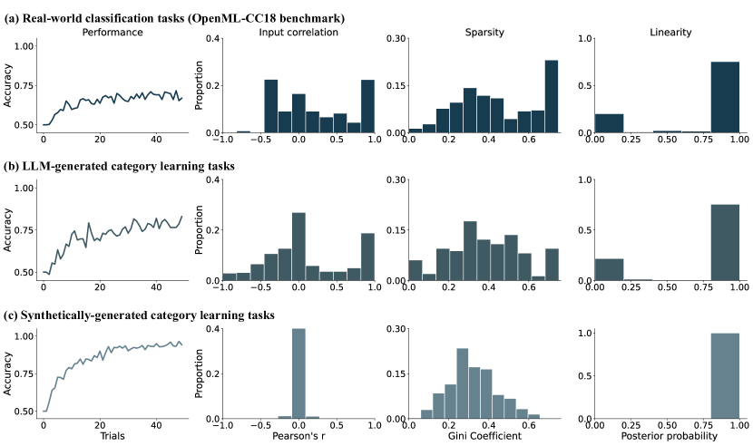
Figure 1: LLM generates ecologically valid category learning tasks: Mean task performance of the logistic regression model measured over trials (first column). Histogram of Pearson’s correlation coefficients computed between pairs of features (second column). Histogram of Gini coefficients computed over the logistic regression weights (third column). Linearity of the category learning task (fourth column) computed for (a) 28 different real-world binary classification tasks from the OpenML-CC18 benchmarking suite (b) ecologically valid category learning tasks generated from Claude-v2 and (c) synthetic category learning tasks derived using the Bayesian logistic regression prior.

3.2 Ecologically rational meta-learned inference (ERMI)

We parsed the generated tasks as described in Appendix A.3 and stored them in a numerical format. Then, we constructed rational learning algorithms for the numerical data by training memory-based meta-learning systems based on a two-stage process (Hochreiter et al., 2001; Santoro et al., 2016; Wang et al., 2016). In an inner-loop stage, a neural network predicts the category $y_{t}$ for an input stimulus $x_{t}$ conditioned on preceding stimulus-category pairs $x_{1:t-1},y_{1:t-1}$. In an outer-loop stage, the network’s parameters $\theta$ are updated using the following objective:

$$\underset{\theta}{\arg\max}~{}\mathbb{E}_{p(x_{1:T},y_{1:T})}\left[\sum_{t=1}^{T}\log p_{\theta}\left(y_{t}\mid x_{1:t},y_{1:t-1}\right)\right]$$ (1)

where $p_{\theta}$ defines the output probabilities produced by the network.

During evaluation – i.e., once training is completed – the neural network implements a free-standing learning algorithm that can predict the category label of a new stimulus based on preceding stimulus-category pairs, despite its parameters being frozen. The resulting network approximates the Bayes-optimal learning algorithm for the data set of the category learning tasks $p(x_{1:T},y_{1:T})$ encountered during training (Ortega et al., 2019).

We refer to the class of models derived by training on ecologically valid (i.e., LLM-generated) category learning task as ecologically rational meta-learned inference (ERMI). If trained on synthetically-generated category learning tasks sampled from a Bayesian logistic regression prior, we refer to the models as meta-learned inference (MI; Binz et al., 2022a). Finally, using the terminology of Müller et al. (2022), we refer to the models as prior-data fitted networks (PFN) when tasks are sampled from a Bayesian neural network prior. For details on how these tasks are generated, see Appendix B.1.

The backbone for all our meta-learning models consisted of a transformer-based decoder architecture (Vaswani et al., 2017) with a causal attention mask. The network had six layers, a model dimension of 64, 256 hidden units in the feed-forward network, and eight attention heads. Positional encoding of input data points was done using sine and cosine functions of different frequencies (Vaswani et al., 2017). Note that during evaluation, transformer weights are frozen and learning is purely driven by self-attention applied to causally masked inputs.

In each training episode, a batch of tasks is sampled from $p(x_{1:T},y_{1:T})$ and the model predicts the category for the given stimulus conditioned on all preceding stimulus-category pairs. Finally, the objective mentioned in Equation 1 is computed, and model parameters are updated using the Adam optimizer (Kingma & Ba, 2014) with a learning rate of $10^{-4}$. This process is repeated for $500\,000$ episodes. We provide full details about the model training procedure in Appendix B.2.

4 LLM-generated category learning tasks are ecologically valid

ERMI can only be interpreted as an ecologically rational model if the statistics of LLM-generated tasks on which it was trained match the statistics of real-world classification problems. We verified that this was the case by comparing the data distributional properties of the two (Chan et al., 2022). For this analysis, we relied on the OpenML-CC18 benchmarking suite, a curated collection of real-world classification tasks (Bischl et al., 2019). Note that although the OpenML-CC18 benchmark is large enough to enable this form of statistical analysis, it is too small for direct meta-learning.

We downsampled all tasks in the OpenML-CC18 benchmark to four feature dimensions and included only binary classification tasks without any missing features in our analysis – amounting to 28 tasks. In addition, we also contrasted LLM-generated tasks to a collection of synthetically-generated category learning tasks with a linear decision boundary (corresponding to those used to train MI). We analyzed these collections of tasks in terms of their learning curves, input correlations, sparsity, and linearity – details for which can be found in Appendix C.

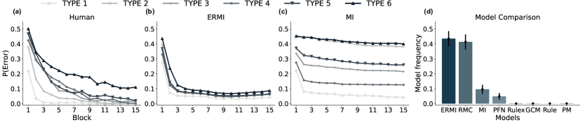
Figure 2: ERMI shows human-like learning difficulties: (a-c) Average error probabilities for each task type in each block of 16 trials for (a) humans, (b) ERMI, and (c) MI. (d) The posterior model frequency of participants’ choices in the Badham et al. (2017) study for eight computational models. Human data in (a) was reproduced from Table 1 in Nosofsky et al. (1994a). ERMI and MI were simulated on type 1-6 tasks for 50 runs with the inverse temperature that resulted in the lowest mean-squared error compared to humans, which was $\beta=0.4$ for ERMI, and $\beta=0.9$ for MI.

Learning curves: Real data is noisy and not perfectly predictable. To investigate whether this is also true for our LLM-generated category learning tasks, we plotted the learning curves of a logistic regression model as a function of the number of training points. We found that the model reaches a ceiling accuracy of around 75% for both LLM-generated and real-world classification tasks (Figure 1; first column). In contrast, the ceiling performance for synthetically-generated tasks was much higher, reaching almost 100%.

Input correlations: Information contained in different feature dimensions are often correlated with each other. In the context of human cognition, it has been argued that this data distributional property of real-world data supports the reliance of people on heuristic decision-making strategies (Gigerenzer & Gaissmaier, 2011). While input dimensions in the synthetically-generated data were not correlated at all, both LLM-generated ($0.11\pm 0.02;\,t(1639)=4.55,\,p<0.001$) and real-world tasks $(0.21\pm 0.01;\,t(2252)=14.64,\,p<0.001)$ showed a significant percentage of correlated features (Figure 1; second column). The corresponding histograms had similar shapes, both containing a peak at perfectly correlated features.

Sparsity: Another data distributional property that allows people to ignore information is sparsity — for many tasks only a few dimensions are relevant. We fitted a linear model on each task to evaluate whether we could find evidence for this in the LLM-generated data. We used the Gini coefficient – a measure borrowed from the economics literature – of the resulting regression coefficients to quantify sparsity (Binz et al., 2022a). High Gini coefficients correspond to maximal sparsity, meaning only a single feature is relevant. Both LLM-generated ($0.38\pm 0.01;\,t(545)=3.81,\,p<0.001$) and real-world tasks ($0.45\pm 0.01;\,t(762)=10.83,\,p<0.001$) exhibited significantly higher sparsity than synthetically-generated tasks ($0.32\pm 0.01$, see Figure 1; third column).

Linearity: People have strong priors towards linear relationships but can also learn non-linear ones given enough examples (Lucas et al., 2015; Brehmer, 1974). To measure whether this bias is also present in the distributional properties of the data, we conducted a model comparison between a linear model (a simple logistic regression model) and a non-linear one (logistic regression with higher-order polynomial features). For each task, we computed the posterior probability that the linear model offers a better explanation as our measure of linearity (details can be found in Appendix C). Most LLM-generated and real-world tasks were found to be linear but there was also a significant number of exceptions (Figure 1; fourth column). The synthetically-generated tasks, on the other hand, were fully linear by design.

Taken together, these analyses indicate that category learning tasks generated by LLMs share many features with real-world classification tasks. As they can also be produced in large quantities, these tasks can serve as a substitute for real-world classification tasks when meta-learning ecologically rational learning algorithms.

5 ERMI shows human-like learning difficulties

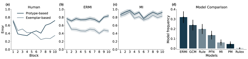
Figure 3: ERMI becomes more exemplar-based with learning: (a-c) The average error of exemplar- and prototype-based models fitted to (a) human choices, (b) simulated choices from ERMI, and (c) simulated choices from MI for each block of 56 trials. (d) The posterior model frequency of participants’ choices in the Devraj et al. (2021) study for seven computational models. Human data in (a) was reproduced from Smith & Minda (1998). ERMI and MI were simulated using inverse temperature values fitted to participants’ choices in Devraj et al. (2021). The mean of the fitted inverse temperature and its standard error were $0.09\pm 0.01$ for ERMI and $0.17\pm 0.02$ for MI, respectively. The shaded region shows the standard error of the mean.

In the following sections, we investigate how well ERMI captures human category learning. We began by looking at one of the most canonical studies in category learning originally conducted by Shepard et al. (1961). The study required participants to learn how to categorize a stimulus that varied in shape (triangle or square), size (small or big), and color (black or white). In total, there were eight stimuli, and participants had to categorize them into one of two categories over several blocks of 16 trials. The authors assigned a stimulus to a category based on six different rules (labeled type 1 to type 6) that increased in difficulty. For more information, we refer to Appendix G.

Shepard et al. (1961) showed that people find tasks belonging to type 1 the easiest and type 6 the hardest, with the average error for type 1 tasks going to zero after four blocks and type 6 tasks remaining at around $10.6\%$ even after 15 blocks (see Figure 2). The average error for type 2 tasks ($3.2\%$) was found to be lower than for type 3 tasks ($6.1\%$), type 4 tasks ($6.5\%$), and type 5 tasks ($7.5\%$).

We simulated ERMI and MI on the Shepard et al. (1961) study. Figure 2 (a) to (c) shows their learning curves alongside those of humans for the six difficulty levels. It can be seen that the learning curves of ERMI are difficulty-dependent and are in terms of mean-squared error (MSE) more similar to humans ($\mathrm{MSE}=0.03$) than MI ($\mathrm{MSE}=0.26$). Notably, ERMI, like humans, finds the type 1 task easier than the type 6 task and shows a similar clustering of learning curves for type 2 to type 5 tasks. However, we also find that ERMI learns much faster than people: its performance plateaus after four blocks while humans continue learning until the end of the experiment for most types. Even though MI performs tasks of different difficulty levels to varying degrees of success, its learning curves do not match those of humans. For example, unlike humans, MI finds type 2 tasks as difficult as type 6 tasks and type 4 tasks easier than type 3 tasks.

Furthermore, we investigated how well ERMI explains human trial-by-trial choices on a quantitative level. For this, we considered human data from Badham et al. (2017) who conducted a replication of Shepard’s original study that only included type 1 to type 4 tasks. We performed a Bayesian model comparison between eight computational models: the three meta-learned models introduced earlier (ERMI, MI, and PFN), and five other cognitive models. The five established category learning models from the cognitive science literature included the rational model of categorization (RMC; Anderson, 1991a), the generalized context model (GCM; Nosofsky, 1986), a prototype model (PM; Homa & Cultice, 1984), a rule-based model (Rule; Ashby & Townsend, 1986), and a rule-plus-exception model (Rulex; Nosofsky et al., 1994b). We provide more details about the five cognitive models, their fitting procedure, and the model comparison in Appendix D, E, and F.

We measured the goodness-of-fit to human choices based on two metrics: posterior model frequency and exceedance probability (Rigoux et al., 2014). The posterior model frequency measures how often a model offers the best explanation in the population, while the exceedance probability measures how likely it is that a given model is the most frequent explanation (the latter is reported in the Appendix G). Figure 2 (d) shows that ERMI explains human choices the best more frequently $(0.43\pm 0.05)$ compared to the other models, with the RMC coming in a close second $(0.41\pm 0.05)$. MI $(0.10\pm 0.03)$ and PFN $(0.05\pm 0.02)$ fit human data the best less than $10\%$ of the time. The classical cognitive models like the exemplar-, prototype- and rule-based models failed at explaining human choices better than other competing models ($\leq 1\%$ of times).

6 ERMI becomes more exemplar-based with learning

What strategy people use to categorize objects and how the application of strategies changes over time are heavily debated questions in psychology. Smith & Minda (1998) attempted to understand whether people use prototype- or exemplar-based strategies during category learning. More specifically, they asked: do people learn a prototype for each category and assign categories based on the similarity of a stimulus to the learned prototypes, or do they instead remember previously seen examples for each category and assign categories based on the similarity of a stimulus to the stored exemplars?

To investigate this, Smith & Minda (1998) designed a category learning task that contained 14 six-dimensional stimuli, each of which was assigned to a category based on a non-linear decision rule. Participants in their experiment were then tasked to assign one of the two categories to repeatedly presented stimuli. Following this, they fit predictions from prototype- and exemplar-based models to proportions of human choices, aggregated over trials within a block, by minimizing the MSE between them. They found that people were better explained by the prototype-based model in the early blocks but in the later blocks, their choices aligned more closely with the exemplar-based model as shown in Figure 3 (a). We provide more details about this analysis in Appendix H.

Figure 4: ERMI displays human-like generalization: (a-c) Average categorization probabilities of transfer stimuli T1-T7 for (a) humans (b) ERMI (c) MI. (d) The encoding scheme used for the seven transfer stimuli. Human data in (a) was reproduced from Johansen & Palmeri (2002). ERMI and MI were simulated on the same experiment for 77 runs, with inverse temperature settings that resulted in the lowest mean-squared error compared to humans, which was $\beta=$ 0.9 for ERMI, and $\beta=$ 0.1 for MI.

We simulated choices from ERMI and MI on the task of Smith & Minda (1998) and fitted the prototype- and exemplar-based models on the simulated choices as in the original study. We find that ERMI, like humans, becomes increasingly exemplar-based over trial segments ($\hat{\beta}=-0.01\pm 0.004;z=-2.54,~{}p<0.01$) whereas choices from MI are explained almost equally well by exemplar-based and prototype-based learning ($\hat{\beta}=-0.002\pm 0.005;z=-0.47,~{}p=0.63$) as shown in Figure 3 (b) and (c). While humans are better explained by prototype-based models for the first five blocks, ERMI is already better explained by an exemplar-based model from the second block onwards. Like in the previous study, this again indicates that ERMI is learning the task faster than humans. Nonetheless, these results demonstrate that training on ecological category learning problems is sufficient for developing an exemplar-based strategy category assignment. We provide additional details and results in Appendix H.

We then evaluated if ERMI also explains human choices better than competing models in this study. To do this, we conducted a model comparison on human data from Devraj et al. (2021) – a replication of the Smith & Minda (1998) study – following the procedure outlined in Section 5. Posterior model frequency in Figure 3 (d) suggests that ERMI explains human choices the best most often ($0.32\pm 0.06$), closely followed by the GCM ($0.24\pm 0.05$) and the rule-based model ($0.20\pm 0.05$).

7 ERMI displays human-like generalization

Having shown that ERMI learns category structures in a human-like way, we next inspect how it generalizes to stimuli unseen during training and whether it displays generalization patterns similar to people. To this end, we zoomed into the study from Johansen & Palmeri (2002), in which participants were instructed to categorize nine four-dimensional stimuli into two categories. The authors then examined how participants generalized to seven transfer stimuli (labeled T1-T7) for which they did not receive feedback during training. In Figure 4 (a), we report the mean probability of participants assigning category A to each of the seven transfer stimuli at the end of the experiment. It can be seen that they assigned stimuli T5, T6, and T7 mostly to category A and T1, T2, T3, and T4 mostly to category B. We provide further details about the paradigm in Appendix I.

We simulate the behavior of ERMI and MI on the Johansen & Palmeri (2002) study and found that ERMI generalizes to unseen stimuli in a human-like way by classifying stimuli T1, T3, and T4 more often as category B and T5, T6, and T7 more often as category A. MI, on the other hand, classified all stimuli except T7 mostly as category B. The Euclidean distance between the choice probabilities of humans and MI ($0.67$) was higher than that between humans and ERMI ($0.29$). The pattern of generalization of ERMI matches humans except for stimulus T2, which is classified at around chance level. Why exactly this is the case remains a question for future work. One possible explanation could relate to the observation that T2 only contains two non-zero features (see Figure 4 (d)) while all other stimuli categorized as B contain three non-zero features.

8 ERMI achieves state-of-the-art performance on machine learning benchmarks

Humans can bring to bear the rich set of priors they have acquired from their everyday interactions to generalize to novel tasks (Tenenbaum & Griffiths, 2001; Griffiths & Tenenbaum, 2006; Lake & Baroni, 2023). Thus far, we have demonstrated how ERMI captures some of these adaptive priors and explains essential aspects of human category learning. This led us to ask whether such a model can also perform well on real-world classification tasks from the machine learning literature.

To investigate this, we evaluated the performance of ERMI on a set of real-world classification tasks from the OpenML-CC18 benchmarking suite (Bischl et al., 2019). We excluded classification tasks with more than two classes, over 100 features, or missing values, resulting in a set of 23 classification tasks. We then compared the performance of ERMI against several baseline models, including logistic regression, a support vector machine (SVM; Cortes & Vapnik, 1995), XGBoost (Chen & Guestrin, 2016), and TabPFN (Hollmann et al., 2023). TabPFN is an off-the-shelf PFN-based model designed for tabular data prediction that has recently shown state-of-the-art performance on an independent large-scale evaluation (McElfresh et al., 2023).

Following the procedure of Müller et al. (2021), we created 20 class-balanced learning problems with 100 data points for each of the selected data sets. We provided 30 input-label pairs to our models for training and evaluated them on the remaining 70 data points. For each data set, we reduced the input dimensionality to four, keeping only the features with the highest F-value to the target variable. We measured the performance on the test set based on two metrics: accuracy and rank.

We found that ERMI is the best model in terms of both mean accuracy ($70.95\%\pm 0.54$) and mean rank ($2.26\pm 0.22$; see Table 4). TabPFN is the second-best model in terms of mean accuracy ($70.51\%\pm 0.63$), while XGBoost is the second-best in terms of mean rank ($2.61\pm 0.30$). We provide the summary of main results in Table 1 and detailed results across all data sets in Appendix J.

The performance gain of ERMI over TabPFN in terms of mean accuracy is in the same range as TabPFN over XGBoost, indicating that the improvement is substantial. In terms of parameters, TabPFN has $64$ times more parameters than ERMI, and on disk, it is around $80$ times larger, suggesting that there is room for further improvement. When compared to a parameter-matched PFN and MI, ERMI shows a significant accuracy boost of $3.5\%$ and $10\%$ respectively.

Table 1: Performance metrics on OpenML-CC18 benchmark.

Mean	SVM	XGBoost	TabPFN	ERMI
Acc.	$69.29\%$	70.17%	$70.51\%$	70.95%
rank	$2.76$	$2.61$	$2.85$	2.26

9 Discussion

Ecological rationality has a long history in cognitive science (Brunswik, 1955; Simon, 1990; Todd & Gigerenzer, 2012). However, it has been notoriously difficult to build models that are optimally adapted to the problems that people encounter in their everyday environment. From a technical perspective, the framework of meta-learning offers a solution to this problem. Yet, it has thus far only been applied to artificially-generated environments (Kumar et al., 2020; Binz & Schulz, 2022b; Binz et al., 2022a; Lake & Baroni, 2023; Jagadish et al., 2023). The main obstacle up to now was that the number of available real-world data sets was insufficient for meta-learning. We have shown that one can overcome this obstacle by prompting LLMs to generate a large collection of ecologically valid category learning tasks. We have then used meta-learning to obtain models that are optimally adapted to them, leading to a class of ecologically rational models that we call ERMI.

ERMI captured three patterns, which are also observed when humans learn to categorize objects: (1) it showed similar learning difficulties as humans, (2) it became more exemplar-based as learning progressed, and (3) it displayed human-like generalization patterns. Furthermore, it explained human behavior better than competing approaches on a quantitative level, thereby suggesting that we can explain many characteristics of human category learning using the principle of ecological rationality.

The methodology developed, more importantly, enables us to test whether people are ecologically rational or not, thereby allowing us to ask questions such as: how much of human learning can be attributed to data distributional properties alone? The approach we have proposed is quite general and in future work, we plan to extend it to other domains, such as decision-making (Bourgin et al., 2019; Peterson et al., 2021), reinforcement learning (Brändle et al., 2021), and function learning (Schulz et al., 2017, 2016). Furthermore, it would be interesting to not impose a predefined task structure on the LLM but instead let it synthesize arbitrary task structures by itself.

However, at the same time, there were also facets of human category learning not captured by ERMI. In particular, we found that ERMI generally learned faster than people. In the third experiment, for instance, ERMI already displayed the generalization patterns shown in Figure 4 after two blocks, while people required 16 blocks or more (Johansen & Palmeri, 2002). We believe that this gap can (at least partially) be closed by incorporating limited computational resources (Binz et al., 2022a; Jagadish et al., 2023) or other architectural constraints (Achterberg et al., 2023).

To conclude, we have shown that LLMs can generate ecologically valid category learning tasks that can be used for meta-learning. With these models at hand, we then demonstrated that one can explain human category learning to a large extent using the principle of ecological rationality. Furthermore, the priors acquired by ERMI are rich enough that it achieves state-of-the-art performance on a real-world classification benchmark. In future work, we plan to scale up ERMI’s architecture, train it on classification tasks with a flexible number of features, increase the maximum number of data points, and allow for more than two classes.

Appendix A Generating ecologically valid category learning tasks using LLMs

A.1 Synthesizing task features and labels

We synthesized task features and labels from claude-v2 using the prompt mentioned in Section 3.1, running it for a total of 100 batches. In each batch, we generate 250 tasks or until a maximum token length of $10$k is reached. We repeat the procedure for all three different stimuli dimensions. In total, we synthesized 23421, 20690, and 13693 category learning tasks with three, four, and six-dimensional features respectively.

We show the counts for the top-50 most frequently occurring task features in Figure 5 and categories in Figure 6 for the 23421, 20690, and 13693 category learning tasks generated with three (a), four (b), and six-dimensional features respectively. We found that the model tends to produce features belonging to topics such as musicality (for instance, rhythm, melody, lyrics, tempo, vocals) and food (for instance, aroma, texture, crust, diet, protein). Regarding categories, there were many related to music (for example, classical, pop, jazz, rock) and vehicles (like trucks, SUVs, sedans). In future work, we plan to do a semantic analysis of the generated task features and category labels using methods such as hierarchical clustering to study the semantic grouping of the generated task features/categories.

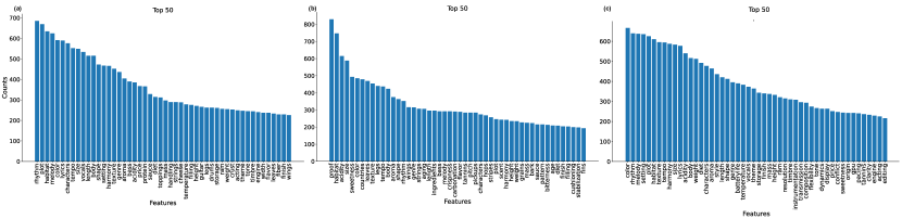
Figure 5: Frequency of different features in claude-v2 synthesized category learning tasks: Counts for the top-50 most frequently occurring task features in the 23421, 20690, and 13693 category learning tasks generated for three (a), four (b), and six-dimensional features respectively.

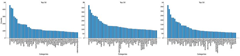
Figure 6: Frequency of different categories in claude-v2 synthesized category learning tasks: Counts for the top-50 most frequently occurring category labels in the 23421, 20690, and 13693 category learning tasks generated for three (a), four (b), and six-dimensional features respectively.

A.2 Generating category learning tasks

We used the prompt mentioned in Section 3.1 to generate data points for task features and labels synthesized in the first stage. We aimed to generate 100, 300, and 616 data points for category learning tasks with stimuli of three, four, and six dimensions respectively. However, sometimes the upper bound of $100$k tokens is reached and the model does not generate the number of data points specified in the prompt. This was especially the case in category learning tasks with higher dimensional stimuli. In these cases, we generate the data points in two steps. In step one, we do the data generation as before using the original prompt. In step two, we query the model again but now conditioned it on the first 20-40 percent of the data points generated in step 1 along with the prompt. This way, we could scale up the generated data points to up around 1.5 times the original length keeping the same underlying data distribution. We generated a total of 11518, 8950, and 12911 category learning tasks with three, four, and six-dimensional stimuli respectively.

Note on other LLMs:

We ran preliminary tests on LLMs other than claude-v2 for generating category learning tasks including LLaMA (Touvron et al., 2023) and GPT-4 (Achiam et al., 2023). The non-instruction-tuned LLaMA version was not able to consistently produce the 100-616 data points we need per task. It was also especially difficult to parse the output of the model as the generated output failed to stick to the provided format. This problem could be mitigated with instruction-tuned versions of LLaMA that are now available but we leave it for future work. We also performed preliminary tests on the GPT-4 model from OpenAI for category learning task generation but found the model sampled the values for the features from uniform distribution using the code module and applied simple heuristic rules most of the time. For example, the sum of two features should be greater than the third and the mean of the two features greater than the other. Upon conducting a preliminary statistical analysis on a relatively small data set generated from GPT-4, we found that task statistics are similar to the statistics of the MI data set, thereby lacking the diversity in terms of measures reported in Section 4.

A.3 Parsing data generated by LLMs

Parsing synthesized task features and labels:

We queried the claude-v2 to synthesize task features and labels in the following format: feature dimension 1, feature dimension 2, …, feature dimension N, category label 1, category label 2. We then used a regular expression (regex) pattern, specifically \d+\.(.+?)\n, to efficiently parse and extract relevant data from the model output. This regex was designed to identify and isolate sequences beginning with a number followed by a period, capturing subsequent characters up to the first newline character. The extracted text was then processed to acquire the names for feature dimensions and category labels by splitting the string at the commas. The final processed data is then stored as a dataframe for future use.

Parsing generated task data points:

We queried the claude-v2 to generate data points for a given category learning task in the following format: - feature value 1, feature value 2,…, feature value N, category label. The model followed the aforementioned format while generating the data points for a category learning task, more often than not. We then used a collection of regular expression (regex) patterns to parse the generated, ensuring accurate handling of different data formats. These regex patterns were designed to cover a wide range of scenarios: capturing numeric values with or without decimal points, handling alphanumeric strings including those with hyphens, and handling complex cases involving commas, hyphens, and optional preceding labels. Furthermore, they extend to different delimiters and formats, from simple comma-separated values to more complex structures with optional components. In Table 2, we show all the regex expressions used to parse data points. Based on these expressions, we were able to successfully parse up to 95 % of the tasks generated by the model. The values extracted from these regex expressions are then stored in a dataframe which acts as an offline repository of tasks on which one can train the ecologically rational meta-learned inference model.

Table 2: Regular expression patterns used for parsing the data points generated for category learning tasks by claude-v2

Index	Regular expression
1	([\d.]+),([\d.]+),([\d.]+),([\w]+)
2	([\w\-]+),([\w\-]+),([\w\-]+),([\w]+)
3	([-\w\d,.]+),([-\w\d,.]+),([-\w\d,.]+),([-\w\d,.]+)
4	([^,]+),([^,]+),([^,]+),([^,]+)
5	([^,\n]+),([^,\n]+),([^,\n]+),([^,\n]+)
6	(?:.*?:)?([^,-]+),([^,-]+),([^,-]+),([^,-]+)
7	([^,-]+),([^,-]+),([^,-]+),([^,-]+)
8	r’^(\d+):([\d.]+),([\d.]+),([\d.]+),([\d.]+),([\w]+)’
9	r’^(\d+):([\w\-]+),([\w\-]+),([\w\-]+),([\w\-]+),([\w]+)’
10	r’^(\d+):([-\w\d,.]+),([-\w\d,.]+),([-\w\d,.]+),([-\w\d,.]+),([-\w\d,.]+)’
11	r’^(\d+):([^,]+),([^,]+),([^,]+),([^,]+),([^,]+)’
12	r’^(\d+):([^,\n]+),([^,\n]+),([^,\n]+),([^,\n]+),([^,\n]+)’
13	r’^(\d+):(?:.*?:)?([^,-]+),([^,-]+),([^,-]+),([^,-]+),([^,-]+)’
14	r’^(\d+):([^,-]+),([^,-]+),([^,-]+),([^,-]+),([^,-]+)’
15	^(\d+):([\d.]+),([\d.]+),([\d.]+),([\d.]+),([\d.]+),([\d.]+),([\w]+)
16	^(\d+):([\w-]+),([\w-]+),([\w-]+),([\w-]+),([\w-]+),([\w-]+),([\w]+)
17	(\d+):([^,]+),([^,]+),([^,]+),([^,]+),([^,]+),([^,]+),([^,]+)
18	(\d+):([^,\n]+),([^,\n]+),([^,\n]+),([^,\n]+),([^,\n]+),([^,\n]+),([^,\n]+)
19	(\d+):(?:.*?:)?([^,-]+),([^,-]+),([^,-]+),([^,-]+),([^,-]+),([^,-]+),([^,-]+)
20	(\d+):([^,-]+),([^,-]+),([^,-]+),([^,-]+),([^,-]+),([^,-]+),([^,-]+)

Appendix B Meta-learned inference models

B.1 Synthetic data generation

Bayesian logistic regression prior used for training MI model:

We generated 10k synthetic binary classification tasks with a linear decision boundary using a Bayesian logistic regression model. To do this, we sample the input features from a normal distribution with zero mean and unit variance for a given number of data points and stimulus dimensions. We then applied a linear transformation, followed by a sigmoid function, and rounded the result to determine the binary class for the given input. The parameters of the linear transformation are sampled from a normal distribution with zero mean and unit variance. The maximum number of data points within a task was set to 400, 650, or 300 for category learning tasks with three, four, and six-dimensional stimuli respectively. These values were chosen depending on the length of the experiments on which these models were evaluated.

Bayesian neural network prior used for training PFN model:

We generated 10k synthetic binary classification tasks using a version of the Bayesian neural network (BNN) prior developed by Müller et al. (2021). We used normally-distributed i.i.d. input features for a given number of data points and stimulus dimensions. We then pass the input through a BNN with two layers with tanh non-linearity and hidden dimensionality of 64. The network weights and biases were sampled from a normal distribution with a mean of zero and standard deviation of 0.1 and subjected to an additional sparsity constraint (i.e., 20 percent of randomly chosen network weights and biases set to zero). The maximum number of data points was once again set to 400, 650, or 300 for category learning tasks with three, four, and six-dimensional stimuli respectively. The model output is passed through a sigmoid function to generate probability estimates which are then rounded to determine the class for the given input.

B.2 Data pre-processing, model architecture, and training

Data pre-processing:

We filter out all tasks with more than two unique category labels and then binarize the category labels which are originally strings to make them consistent across tasks. We also normalized each feature independently using a min-max normalization scheme such that values taken by any feature lie always between zero and one. Both the task features and data points were shuffled while generating tasks. Note that the tasks generated by LLMs are typically of different lengths. Whenever the sampled tasks are of variable lengths, they are padded with zeros to match the length of the longest task sample within the batch. We additionally also sampled LLM-generated data points with replacement to match the length of the experimental task used in the Devraj et al. (2021) and Johansen & Palmeri (2002) studies. We resorted to this strategy as the LLM-generated tasks had a maximum of about 200 data points per task and by resampling, we can evaluate the model on experiments with larger horizons without any drop in performance. The batch size was set to 64 for three- and four-dimensional stimuli and to 32 for six-dimensional stimuli and it operated under a maximum steps regime of 400, 300, and 650 for three, four, and six-dimensional tasks respectively.

Model architecture and training:

The task features were mapped onto a 64-dimensional embedding space and positional encoded using sine and cosine functions of different frequencies as in Vaswani et al. (2017). A casual attention mask was then generated for the inputs such that the model makes conditional predictions on all preceding data points. The inputs along the attention mask are then passed to the transformer decoder model which had six layers, a model dimension of 64, 256 hidden units in the feed-forward network, and eight attention heads. The output of the transformer was then passed through a linear readout and sigmoid function to generate probability estimates for category 1. In practice, inference for all time steps is performed in parallel by passing a causal attention mask to the TransformerDecoder module in PyTorch (Paszke et al., 2019). We used binary cross-entropy (BCE) loss for a given batch of inputs and updated the model parameters using the ADAM optimizer (Kingma & Ba, 2014) with a learning rate of $10^{-4}$. We trained all our models for a total of $500\,000$ episodes.

Appendix C LLMs generate ecologically valid category learning tasks

Sparsity:

We fitted a logistic regression model for each task and analyzed the sparsity of the resulting regression weights $\mathbf{w}\in\mathbb{R}^{d}$ using the Gini coefficient $G$:

$$G(\mathbf{w})=\dfrac{\displaystyle\sum\limits_{i=1}^{d}\displaystyle\sum\limits_{j=1}^{d}|\mathbf{w}_{i}-\mathbf{w}_{j}|}{2d\displaystyle\sum\limits_{i=1}^{d}\mathbf{w}_{i}}$$ (2)

Linearity:

We fitted a logistic regression model and a logistic regression with second-order polynomial features on data $\mathcal{D}$ from each task. We then computed the Bayesian information criterion (BIC) for both models and used them to approximate the posterior probability that the linear model offers a better explanation of the data (assuming a uniform prior over models):

$$p(M={\text{linear}}|\mathcal{D})\approx \frac{\exp(-0.5\cdot\text{BIC}_{\text{linear}})}{\sum_{m\in\{\text{linear, polynomial}\}}\exp(-0.5\cdot\text{BIC}_{m})}$$ (3)

Appendix D Cognitive models

In this section, we will provide details regarding the five cognitive models we used for model comparison.

Rational model of categorization (RMC):

The RMC is a Bayesian model of human category learning (Anderson, 1991a). In this paper, we used a meta-learned version of the model, which was obtained using the following data-generating distribution described in Badham et al. (2017). Model architecture and training followed the protocol used for ERMI, MI, and PFN. We set the free parameters based on an earlier study (Nosofsky et al., 1994a) to the following values: $c=0.318$, $s_{P}=0.488$, and $s_{L}=0.046$. Note that we did not account for these parameters in our model comparisons, which slightly overestimates the ability of the RMC to explain human behavior.

Prototype-based model (PM):

There are several versions of the prototype model (Medin & Schaffer, 1978; Smith & Minda, 1998). Here, we use the version from Smith & Minda (1998). The prototype model assigns a category to an observed stimulus based on the similarity to the category prototypes. The raw distance between the stimulus and a prototype, $q_{k}$, for category $k$ is computed as a weighted sum of absolute differences across $n$ feature dimensions with weights, $w_{j}\in[0,1]$, for the features contained to sum to 1 as shown in Equation 4.

$$d_{x,q_{k}}=\sum_{j=1}^{n}w_{j}\left|x_{j}-q_{k,j}\right|,$$ (4)

Note that prototypes themselves can either be learned or provided during model definition. Here, we learn the prototypes for the two categories $\{q_{1},q_{2}\}$. Therefore, $q_{k,j}\in[0,1.]~{}\forall j=\{1,2,...n\}$ are themselves also parameters. Distance is then converted to psychological similarity between prototypes and stimuli using:

$$\eta_{x,q_{k}}=e^{-c\cdot d_{x,q_{k}}}$$ (5)

where $c$ is a sensitivity parameter that can shrink or amplify discriminability in psychological space. The probability of the stimulus being assigned to category $1$ is then computed using:

$$P(k=1\mid x)=\frac{\eta_{x,q_{1}}}{\eta_{x,q_{1}}+\eta_{x,q_{2}}}$$ (6)

Furthermore, the final model predicted likelihood is a mixture between the predicted probability from the model and a random guess, with guessing parameter $\epsilon$ controlling the mixture probabilities:

$$p(k=1\mid x)=(1-\epsilon)P(k=1\mid x)+\epsilon\cdot\mathrm{K}^{-1}$$ (7)

where $\mathrm{K}$ indicates number of categories.

Generalized context model (GCM):

We used the GCM developed by Nosofsky (1986). The GCM categorizes an observed stimulus to a category by comparing the sum of its similarity to all previously seen exemplars in each category, $\{C_{1},C_{2}\}$. The raw distance and similarity between observed stimulus and exemplars were computed based on Equations 4 and 5 respectively. The probability of assigning a stimulus to category $k=1$ is then computed based on the summed category similarities in the following way:

$$P(k=1\mid x)=\frac{\sum_{y\in C_{1}}\eta_{x,y}}{\sum_{y\in C_{1}}\eta_{x,y}+\sum_{y\in C_{2}}\eta_{x,y}}$$ (8)

The final model predicted category probabilities is again a mixture between the predicted probability from the model and a random guess as mentioned in Equation 7.

Rule (Rule):

The rule model implemented in this work assigns a category based on one of the two rules, whichever explains the participant data better. The first rule is based on the values taken by stimulus features along one dimension, and the second is based on the application of the conjunctive rule on pairs of features – whether a given pair of stimulus features take on the same value. The final model predicted category probabilities is again a mixture between the category prediction from the model and a random guess as mentioned in Equation 7.

Rule plus exception model (Rulex):

We use the same implementation as the Rule model but provide exceptions as inputs to the model. For Devraj et al. (2021) task, we provide $[1,1,1,1,0,1]$ as the exception stimulus for category 1, and for category 2, it was set to $[0,0,0,1,0,0]$. For Badham et al. (2017) task, we provide $[1,1,1]$ and $[0,0,0]$ as exceptions for type-2 task. The final model predicted category probabilities is again a mixture between the category prediction from the model and a random guess as mentioned in Equation 7. In future work, we plan to implement a more detailed version of rule-plus-exception model from (Nosofsky et al., 1994b) where the model learns the exceptions along with the rule.

Appendix E Fitting models to human data

In this section, we explain the fitting procedure used to fit the parameters of the models to human data. The model parameters were fit to the data using maximum likelihood estimation. We explain the implementation details for the different model classes below. The full list of fitted parameters for each model is shown in Table 3.

MI, PFN, RMC and ERMI:

We fit an inverse temperature term $\beta$ within the sigmoid function, which squashes the output from the final layer of the transformer to be within $[0,1]$, to each participant. Note that this term is set to one during the meta-learning phase to derive an optimal model and is fitted only during the evaluation phase with the rest of the model weights being frozen. We use the differential evolution optimizer available in the SciPy optimization library (Virtanen et al., 2020) for fitting.

GCM and PM:

Both models predict the probability of picking a category in a trial-by-trial fashion conditioned on all preceding stimulus-target pairs. We fit their parameters to human choices that minimize the negative log-likelihood of human choices under the model prediction. To do so, we used the minimize module available in SciPy’s optimization library. As mentioned in Section D, the weights for the features were bounded to be within $[0,1]$ and sum to 1, the sensitivity term bounded to be within $[0,20]$. The prototype model requires learning the prototypical stimulus for each category (same dimensionality as the input stimulus, with the feature values bounded to be within $[0,1]$). Both models learning a guessing parameter $\epsilon$, which was bounded to be within $[0,1]$.

Rule and Rulex:

We used the same procedure as above except that we learn the stimulus dimension $v_{i}$ on which the rule is applied.

Table 3: Fitted parameters in each model where $\beta$ is the inverse temperature term, $w_{i}$ indicates the weights for the stimulus feature dimension $i$, $n$ is the number of stimulus feature dimensions, $c$ is the sensitivity term, $\epsilon$ is noise term in an epsilon greedy policy, $q_{1}$ and $q_{2}$ are the values for the prototypes for $d$ stimulus features, and $v_{i}$ are the stimulus dimension on which the rule is applied.

Model	Parameters
ERMI, MI, PFN, RMC	$\beta$
GCM	$c,\epsilon,w_{i}$	$\forall~{}i\in\{1,2,\ldots,n\}$
PM	$c,\epsilon,w_{i},q_{1,i},q_{2,i}$	$\forall~{}i\in\{1,2,\ldots,n\}$
Rule	$v_{1},v_{2},\epsilon$
Rulex	$v_{1},v_{2},\epsilon$

Appendix F Bayesian model comparison

In this section, we provide details regarding the Bayesian model comparison procedure used to compare the fits of different models to the behavioral data. We first performed maximum likelihood estimation to fit model parameters $\theta_{m}$. We then computed the Bayesian information criterion (BIC) for model $m$ for a given participant as follows:

$$\text{BIC}_{m}=-2\cdot\max_{\theta_{m}}\sum_{t=1}^{T}\log p_{\theta_{m}}\left(\hat{y_{t}}\mid x_{1:t},y_{1:t-1}\right)+|\theta_{m}|\log(T)$$ (9)

where $|\theta_{m}|$ is the number of parameters estimated for model $m$, $T$ is the number of trials in the task and $\hat{y_{t}}$ is the category choice made by the participant in trial $t$. BIC penalizes the model based on its complexity and can be used as a measure for comparing goodness-of-fit when models differ in terms of their number of parameters.

We reported two metrics in the paper: posterior model frequency (in the main text) and exceedance probability. To compute them, we used a Python implementation of the Variational Bayesian Analysis (VBA) toolbox (Daunizeau et al., 2014). The toolbox requires us to provide log-evidences for each model and participant, which we approximate using $-0.5\cdot\text{BIC}_{m}$. For further details about this model comparison procedure, see Rigoux et al. (2014).

Appendix G ERMI shows human-like difficulty effects

G.1 Experiment details for Shepard et al. (1961) and Nosofsky et al. (1994a)

In their replication of the Shepard et al. (1961) study, Nosofsky et al. (1994a) conducted the study on 120 participants. The authors used geometric stimuli that varied in shape (squares or triangles), interior line type (solid or dotted), and size (large or small). Every participant completed two problems, therefore, each problem was performed by 40 participants. The participants were informed that the rules for each problem were independent. Following the methodology of Shepard et al. (1961), the learning process involved classifying stimuli into two categories and receiving feedback. This process was repeated over several blocks (containing up to 16 trials) with randomized stimulus order in each block. Learning in the task was measured until participants achieved a no-error streak in four consecutive sub-blocks of eight trials or reached a maximum of 400 trials. For more details, please refer to Nosofsky et al. (1994a).

In tasks belonging to type 1, stimuli were assigned to a category depending on the values they take along one of the three dimensions, whereas in type 2 tasks, stimuli were assigned to a category by applying the exclusive-or rule along two relevant dimensions. Category assignment in tasks belonging to type 3, type 4, and type 5 used a unidimensional rule-plus-exception structure with some stimuli grouped in the central region and some in the periphery. Lastly, type 6 tasks require considering feature values along all dimensions. For the illustration of category structures for the six types, please refer to Figure 1 in (Nosofsky et al., 1994a).

In Badham et al. (2017), the authors replicated the Shepard et al. (1961) study on 96 adults aged between 18 to 87 years. They used eight geometric shapes varying in size (large or small), shape (square or triangle), and color (black or white) in the experiment with the stimuli shown on a mid-gray background. The order of stimuli and their category assignment were randomized. They only considered the first four types from the Shepard et al. (1961) study but unlike their study, participants performed all four types. Participants performed each task type for a total of six blocks with each block containing 16 trials (resulting in a total of 96 trials) or until they reached a criterion of perfect performance in two consecutive blocks. For more details, please refer to Badham et al. (2017).

G.2 Simulations:

To run simulations of the Shepard et al. (1961) study on ERMI, MI, and PFN model, the geometric stimuli used in the experiment as mentioned above are converted into binary coded vectors taking values along the three stimulus feature dimensions. The value assignment for a stimulus feature was randomized in every run, the order of presentation of the stimulus was also randomized, and the number of presentations of a stimulus per block was matched to the original study. In each run, the model was evaluated on a task of one particular type.

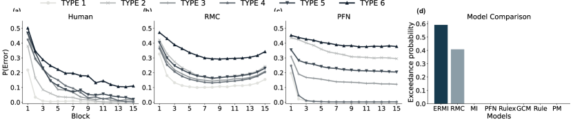
Figure 7: Supplementary figure accompanying Figure 2: (a-c) Average error probabilities for each task type in each block of 16 trials for (a) humans, (b) RMC, and (c) PFN. (d) The exceedance probability of participants’ choices in the Badham et al. (2017) study for eight computational models. Human data in (a) was reproduced from Table 1 in Nosofsky et al. (1994a). RMC and PFN were simulated on type 1-6 tasks for 50 runs with the inverse temperature that resulted in the lowest mean-squared error compared to humans, which was $\beta=0.9$ for ERMI, and $\beta=0.9$ for MI.

G.3 Additional observations and results

Why are type 2 and type 6 hard?

We think that this could be because type 2 tasks involve applying the exclusive-or rule along two relevant dimensions (and ignoring one of the dimensions altogether), while type 6 tasks require memorizing feature values taken by stimuli along all dimensions, making it hard for models to learn.

Learning curves of RMC and PFN are not as similar to humans as ERMI:

MSE between learning curves of humans and RMC and PFN was $0.10$ and $0.17$ respectively. They are larger than that of ERMI which was $0.03$.

ERMI learns the task faster than people:

We transform the block variable $t$ using an exponential kernel as follows:

$$y=ae^{-b*t}+c$$ (10)

where $a$ is the amplitude, $b$ is the decay coefficient term, and $c$ is the offset term, and then regressed the transformed variable onto the error rate for both ERMI and humans. We found that the fitted decay coefficient for ERMI ($1.24$) is larger than for humans ($0.44$).

Baseline models fit the data adequately:

Baseline models particularly the GCM $(177.35\pm 4.70)$ and PM $(201.19\pm 3.38)$ model did fit the data quite well in terms of log-likelihoods compared to ERMI $(200.82\pm 4.56)$. However, the number of parameters being fit to human data is quite large in these models (refer to Table 3). Therefore, they are heavily penalized and have higher BIC values than ERMI.

Appendix H ERMI becomes more exemplar-based

H.1 Experiment details for Smith & Minda (1998) and Devraj et al. (2021)

Smith & Minda (1998) conducted their study on 32 participants, using 14 six-dimensional stimuli, with each stimulus mapping to a six-letter nonsensical word such as gafuzi, kafitdo, nivety, wysero, etc. — see Appendix A of Smith & Minda (1998) for all words. Each stimulus can be represented by a six-digit binary string, where each digit and position corresponds to a specific letter. For example, if the stimulus ’gafuzi’ corresponds to the binary code ’000000’, then ’gyfuzi’ corresponds to ’010000’, and so on. The stimuli were assigned to categories such that stimulus ’000000’ corresponds to category 1 and stimulus ’11111’ corresponds to category 2. We only considered the non-linearly separable (NLS) category structure from Experiment 2 in this work. According to this, a category contained five stimuli with five features in common with the prototype, and one stimulus with five features in common with the opposing prototype. Therefore, category 1 contained seven stimuli as follows: [000000, 100000, 010000, 001000, 000010, 000001, 111101]. The remaining seven stimuli belonged to category 2 [111111, 011111, 101111, 110111, 111011, 111110, 000100]. Participants had unlimited time to make their choice on each trial. After making their choice, they were told whether it was a correct decision or not. Participants completed a total of 560 trials, or 10 blocks (called trial segments by the authors but we call them blocks to be consistent with other experiments) of 56 trials each, in which they saw each stimulus four times.

Devraj et al. (2021) replicated the task as mentioned above and collected data from 60 participants. Participants were recruited from the 18-23 age range and English-speaking population using Prolific. Their study involved 11 blocks instead of 10 and as a result, they had 616 trials.

H.2 Model-based analysis:

The 616 choices made by participants and meta-learning models were divided into 11 blocks of 56 trials each. We obtained the choices from the models – ERMI, MI, and PFN – by simulating them on the task for a total of 50 runs using the $\beta$s fitted to participants in the Devraj et al. (2021) study. We then fit prototype- and exemplar-based models onto the choices of humans and models to see if they are better explained by prototype or exemplar-based strategy. To fit their parameters, we minimize the sum of squared errors (SSE) between observed and predicted probabilities for each participant for a given block following the original study’s approach:

$$SSE=\sum_{t=1}^{14}(p(k=1|x_{t})-\hat{p}_{1,x_{t}})^{2}$$ (11)

where $p(k=1|x_{t})$, from Equation 7, is the predicted probability from the model – either GCM or PM – that stimulus $x_{t}$ belongs to category 1 based on an entire trial segment (56 trials) of data, and $\hat{p}_{1,x_{t}}$ is the proportion of trials in the trial segment (out of those in which stimulus $x_{t}$ was seen) in which the participant or model categorized stimulus $x_{t}$ to category 1. We used SciPy’s Sequential Least Squares Programming (SLSQP) method in the SciPy’s optimization module to obtain the best fitting parameter for the two models as in (Devraj et al., 2021). We then compared the SSE computed using the best-fitting parameters between the two models as shown in Figure 3(a).

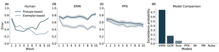
Figure 8: Supplementary material accompanying Figure 3:(a-c) The average error of exemplar- and prototype-based models fitted to (a) human choices, (b) simulated choices from ERMI, and (c) simulated choices from PFN for each block of 56 trials. (d) The exceedance probability of participants’ choices in the Devraj et al. (2021) study for seven computational models. Human data in (a) was reproduced from Smith & Minda (1998). ERMI and MI were simulated using inverse temperature values fitted to participants’ choices in Devraj et al. (2021). The mean of the fitted inverse temperature and its standard error were $0.09\pm 0.01$ for ERMI and $0.14\pm 0.01$ for MI, respectively. The shaded region shows the standard error of the mean.

H.3 Additional observations and results

ERMI is better explained by the exemplar-based model with learning:

We fit a linear mixed-effects model to measure this effect quantitatively. We predict the average error term from the GCM and PM model using blocks and model as predictors and test the interaction between blocks and model. Blocks (1-10) were mean-centered and the exemplar model (GCM) was coded as $-1$ and the prototype-based model (PM) was coded as 1. We report the coefficient $\hat{\beta}$ for the interaction term in the main paper. We found that ERMI ($\hat{\beta}=-0.01\pm 0.004;z=-2.54,~{}p<0.01$) is better explained by the exemplar-based model with learning whereas choices from MI are explained equally well by exemplar-based and prototype-based learning ($\hat{\beta}=-0.002\pm 0.005;z=-0.47,~{}p=0.63$) as shown in Figure 3

Prototype model cannot learn exceptions:

Given that the category structure is non-linearly separable (containing exceptions), a prototype model cannot explain the data fully even if provided the true category choices as it tends to miscategorize the exception stimulus from which category. The exemplar-based model (GCM) model, however, has no such issues and can fit the true choices perfectly.

MI and PFN models find it hard to learn exceptions:

A better fit of the prototype model to the MI and PFN in the latter half of the experiment (as shown in Figure 3 and 8) suggests that, as observed in Shepard’s task, they are not able to learn exceptions like the prototype model as mentioned before.

Appendix I ERMI shows human-like generalization

I.1 Experiment details for Johansen & Palmeri (2002)

Johansen & Palmeri (2002) conducted their study with 198 participants (out of which 68 were excluded for further analysis) using four-dimensional stimuli with each dimension taking one of two possible values. The stimuli were computer-generated drawings of rockets that varied along four binary-valued dimensions: The shape of the wing (triangular or rectangular), tail (jagged or boxed), nose (staircase or half-circle), and porthole (circular or star) (Johansen & Palmeri, 2002). The category structure used in the study was similar to the ones used in classical studies such as Medin & Schaffer (1978); Nosofsky et al. (1994b) and is ill-defined in that no single feature along a dimension can be used to perfectly classify stimuli. Rather, the categories have a family resemblance structure in that category A stimuli tend to have a value of 0 along each dimension, and category B stimuli tend to have a value of 1 along each dimension. In this case, category 1 contained five stimuli as follows: [0001, 0101, 0100, 0010, 1000]. The remaining four stimuli belonged to category 2 [0011, 1001, 1110, 1111]. The stimulus presentation order was randomized within each block. Participants had unlimited time to make their choice on each trial. After making their choice, they were told whether or not it was a correct choice. Participants completed a total of 288 training trials, or 32 blocks of 9 trials each, in which they saw each stimulus once. However, in addition to the training block, participants had to perform a transfer block after 2, 4, 8, 16, 24, and 32 blocks of training. In a transfer block, all 16 possible stimuli are shown without any corrective feedback.

I.2 Simulations

We simulated ERMI, MI, and PFN on the Johansen & Palmeri (2002) study for different betas values, from zero to one in steps of 0.1, for a total of 544 runs. The models interacted with each of the nine training stimuli 32 times with the ordering of the stimuli shuffled between runs. Predictions for the transfer stimuli were derived by concatenating them – one at a time – at the end of 32 training blocks in every run. By doing so, we were able to derive the model’s prediction for each unseen stimulus around $77$ times. In Figure 4 and 9, we reported average choice probabilities for the models using the $\beta$-term that minimized the pair-wise Euclidean distance between the human and model’s choice probabilities.

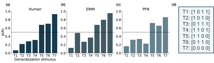
Figure 9: Supplementary material accompanying Figure 4: (a-c) Average categorization probabilities of transfer stimuli T1-T7 for (a) humans (b) ERMI (c) PFN. (d) The encoding scheme used for the seven transfer stimuli is provided for reference. Human data in (a) was reproduced from Johansen & Palmeri (2002). ERMI and MI were simulated on the same experiment for 77 runs, with inverse temperature settings that resulted in the lowest mean-squared error compared to humans, which was $\beta=$ 0.9 for ERMI, and $\beta=$0.1 for PFN.

Table 4: Detailed performance metrics of different models on OpenML-CC18 benchmarking suite.

Data set	Log. Reg.	SVM	XGBoost	TabPFN	ERMI
kr-vs-kp classification	0.8257	0.8514	0.7986	0.8664	0.8450
credit-g classification	0.6421	0.6357	0.6350	0.6036	0.6150
diabetes classification	0.6771	0.7079	0.6786	0.6886	0.6950
spambase classification	0.5407	0.7664	0.7536	0.7993	0.7757
tic-tac-toe classification	0.5536	0.5950	0.6071	0.5914	0.6071
electricity classification	0.5543	0.6007	0.7036	0.6871	0.6436
pc4 Software defect prediction	0.7136	0.7521	0.7886	0.7707	0.7714
pc3 Software defect prediction	0.6514	0.7264	0.7357	0.7279	0.7107
kc2 Software defect prediction	0.5893	0.7314	0.7257	0.7257	0.7257
kc1 Software defect prediction	0.6271	0.6707	0.6743	0.6679	0.6521
pc1 Software defect prediction	0.5336	0.5964	0.6514	0.6064	0.6493
wdbc classification	0.9121	0.9207	0.9014	0.9221	0.9093
phoneme classification	0.5793	0.7314	0.6979	0.6921	0.7200
qsar-biodeg classification	0.5779	0.7014	0.6850	0.6921	0.7064
ilpd classification	0.5493	0.6386	0.6229	0.6121	0.6286
ozone-level-8hr classification	0.6614	0.6907	0.6707	0.6471	0.6950
banknote-authentication classification	0.7721	0.9229	0.8457	0.9657	0.9379
blood-transfution-service-center	0.4714	0.5493	0.5879	0.5671	0.6186
phishing websites classification	0.7929	0.8071	0.8157	0.8157	0.8129
bank-marketing classification	0.5829	0.5614	0.7386	0.7350	0.7171
wilt classification	0.5171	0.5736	0.6393	0.6371	0.6507
numerai28.6 classification	0.4857	0.4779	0.5029	0.4779	0.4986
churn classification	0.6321	0.7271	0.6800	0.7186	0.7329
Mean Acc.	$62.80\pm 0.66$	$69.29\pm 0.62$	70.17$\%\pm 0.52$	$70.51\%\pm 0.63$	70.95$\%\pm$ 0.54
Mean rank	$4.52\pm 0.21$	$2.76\pm 0.26$	$2.61\pm 0.30$	$2.85\pm 0.27$	2.26 $\pm$ 0.22

Appendix J Benchmarking on OpenML-CC18

Table 4 contains the full set of results for all tasks and models.

Appendix K Data and materials

We will make all experimental data and code for this project available under the following link: [RETRACTED].

References

- Achiam et al. (2023) Achiam, J., Adler, S., Agarwal, S., Ahmad, L., Akkaya, I., Aleman, F. L., Almeida, D., Altenschmidt, J., Altman, S., Anadkat, S., et al. Gpt-4 technical report. arXiv preprint arXiv:2303.08774, 2023.
- Achterberg et al. (2023) Achterberg, J., Akarca, D., Assem, M., Heimbach, M., Astle, D. E., and Duncan, J. Building artificial neural circuits for domain-general cognition: a primer on brain-inspired systems-level architecture. arXiv preprint arXiv:2303.13651, 2023.
- Anderson (1991a) Anderson, J. R. The adaptive nature of human categorization. Psychol. Rev., 98(3):409–429, July 1991a. ISSN 0033-295X, 1939-1471. doi: 10.1037/0033-295X.98.3.409.
- Anderson (1991b) Anderson, J. R. Is human cognition adaptive? Behavioral and brain sciences, 14(3):471–485, 1991b.
- Anthropic (2023) Anthropic, P. B. C. Claude 2. https://www.anthropic.com/index/claude-2, July 2023. Accessed: 2024-1-15.
- Ashby & Maddox (2005) Ashby, F. G. and Maddox, W. T. Human Category Learning. Annual Review of Psychology, 56(1):149–178, February 2005. ISSN 0066-4308, 1545-2085. doi: 10.1146/annurev.psych.56.091103.070217. URL https://www.annualreviews.org/doi/10.1146/annurev.psych.56.091103.070217.
- Ashby & Townsend (1986) Ashby, F. G. and Townsend, J. T. Varieties of perceptual independence. Psychological Review, 93(2):154–179, 1986. ISSN 1939-1471. doi: 10.1037/0033-295X.93.2.154. Place: US Publisher: American Psychological Association.
- Badham et al. (2017) Badham, S. P., Sanborn, A. N., and Maylor, E. A. Deficits in category learning in older adults: Rule-based versus clustering accounts. Psychol. Aging, 32(5):473–488, August 2017. ISSN 0882-7974, 1939-1498. doi: 10.1037/pag0000183.
- Bai et al. (2022) Bai, Y., Kadavath, S., Kundu, S., Askell, A., Kernion, J., Jones, A., Chen, A., Goldie, A., Mirhoseini, A., McKinnon, C., et al. Constitutional ai: Harmlessness from ai feedback. arXiv preprint arXiv:2212.08073, 2022.
- Barker (1968) Barker, R. G. Ecological psychology: Concepts and Methods for Studying the Environment of Human Behavior. Stanford, CA: Stanford University Press, 1968.
- Binz & Schulz (2022b) Binz, M. and Schulz, E. Modeling human exploration through resource-rational reinforcement learning. Advances in Neural Information Processing Systems, 35:31755–31768, 2022b.
- Binz et al. (2022a) Binz, M., Gershman, S. J., Schulz, E., and Endres, D. Heuristics from bounded meta-learned inference. Psychological review, 2022a.
- Binz et al. (2023) Binz, M., Dasgupta, I., Jagadish, A., Botvinick, M., Wang, J. X., and Schulz, E. Meta-learned models of cognition. arXiv preprint arXiv:2304.06729, 2023.
- Bischl et al. (2019) Bischl, B., Casalicchio, G., Feurer, M., Hutter, F., Lang, M., Mantovani, R. G., van Rijn, J. N., and Vanschoren, J. Openml benchmarking suites. arXiv:1708.03731v2 [stat.ML], 2019.
- Borisov et al. (2022) Borisov, V., Seßler, K., Leemann, T., Pawelczyk, M., and Kasneci, G. Language models are realistic tabular data generators. arXiv preprint arXiv:2210.06280, 2022.
- Bourgin et al. (2019) Bourgin, D. D., Peterson, J. C., Reichman, D., Russell, S. J., and Griffiths, T. L. Cognitive model priors for predicting human decisions. In International conference on machine learning, pp. 5133–5141. PMLR, 2019.
- Brändle et al. (2021) Brändle, F., Binz, M., and Schulz, E. Exploration beyond bandits. The drive for knowledge: The science of human information seeking, pp. 147–168, 2021.
- Brehmer (1974) Brehmer, B. Hypotheses about relations between scaled variables in the learning of probabilistic inference tasks. Organizational Behavior and Human Performance, 11(1):1–27, 1974.
- Brunswik (1955) Brunswik, E. Representative design and probabilistic theory in a functional psychology. Psychological review, 62(3):193, 1955.
- Chan et al. (2022) Chan, S., Santoro, A., Lampinen, A., Wang, J., Singh, A., Richemond, P., McClelland, J., and Hill, F. Data distributional properties drive emergent in-context learning in transformers. Advances in Neural Information Processing Systems, 35:18878–18891, 2022.
- Chen & Guestrin (2016) Chen, T. and Guestrin, C. Xgboost: A scalable tree boosting system. In Proceedings of the 22nd acm sigkdd international conference on knowledge discovery and data mining, pp. 785–794, 2016.
- Coda-Forno et al. (2023) Coda-Forno, J., Binz, M., Akata, Z., Botvinick, M., Wang, J. X., and Schulz, E. Meta-in-context learning in large language models. arXiv preprint arXiv:2305.12907, 2023.
- Cortes & Vapnik (1995) Cortes, C. and Vapnik, V. Support-vector networks. Machine learning, 20:273–297, 1995.
- Daunizeau et al. (2014) Daunizeau, J., Adam, V., and Rigoux, L. Vba: a probabilistic treatment of nonlinear models for neurobiological and behavioural data. PLoS computational biology, 10(1):e1003441, 2014.
- Devraj et al. (2021) Devraj, A., Zhang, Q., and Griffiths, T. The dynamics of exemplar and prototype representations depend on environmental statistics. In Proceedings of the Annual Meeting of the Cognitive Science Society, volume 43, 2021.
- Gigerenzer & Gaissmaier (2011) Gigerenzer, G. and Gaissmaier, W. Heuristic decision making. Annual review of psychology, 62:451–482, 2011.
- Griffiths et al. (2008) Griffiths, T., Kemp, C., and B Tenenbaum, J. Bayesian models of cognition. Carnegie Mellon University, 2008.
- Griffiths & Tenenbaum (2006) Griffiths, T. L. and Tenenbaum, J. B. Optimal predictions in everyday cognition. Psychological science, 17(9):767–773, 2006.
- Griffiths et al. (2023) Griffiths, T. L., Zhu, J.-Q., Grant, E., and McCoy, R. T. Bayes in the age of intelligent machines. arXiv preprint arXiv:2311.10206, 2023.
- Gunasekar et al. (2023) Gunasekar, S., Zhang, Y., Aneja, J., Mendes, C. C. T., Del Giorno, A., Gopi, S., Javaheripi, M., Kauffmann, P., de Rosa, G., Saarikivi, O., et al. Textbooks are all you need. arXiv preprint arXiv:2306.11644, 2023.
- Hammond (1998) Hammond, K. R. Ecological validity: Then and now, 1998.
- Hochreiter et al. (2001) Hochreiter, S., Younger, A. S., and Conwell, P. R. Learning to learn using gradient descent. In Artificial Neural Networks—ICANN 2001: International Conference Vienna, Austria, August 21–25, 2001 Proceedings 11, pp. 87–94. Springer, 2001.
- Hollmann et al. (2023) Hollmann, N., Müller, S., Eggensperger, K., and Hutter, F. TabPFN: A transformer that solves small tabular classification problems in a second. In The Eleventh International Conference on Learning Representations, 2023. URL https://openreview.net/forum?id=cp5PvcI6w8_.
- Homa & Cultice (1984) Homa, D. and Cultice, J. C. Role of feedback, category size, and stimulus distortion on the acquisition and utilization of ill-defined categories. Journal of Experimental Psychology: Learning, Memory, and Cognition, 10(1):83, 1984.
- Jagadish et al. (2023) Jagadish, A. K., Binz, M., Saanum, T., Wang, J. X., and Schulz, E. Zero-shot compositional reinforcement learning in humans. PsyArXiv preprint PsyArXiv:ymve5, 2023.
- Jensen et al. (2023) Jensen, K. T., Hennequin, G., and Mattar, M. G. A recurrent network model of planning explains hippocampal replay and human behavior. bioRxiv, pp. 2023–01, 2023.
- Johansen & Palmeri (2002) Johansen, M. K. and Palmeri, T. J. Are there representational shifts during category learning? Cogn. Psychol., 45(4):482–553, December 2002. ISSN 0010-0285. doi: 10.1016/s0010-0285(02)00505-4.
- Kingma & Ba (2014) Kingma, D. P. and Ba, J. Adam: A method for stochastic optimization. arXiv preprint arXiv:1412.6980, 2014.
- Kumar et al. (2020) Kumar, S., Dasgupta, I., Cohen, J., Daw, N., and Griffiths, T. Meta-learning of structured task distributions in humans and machines. In International Conference on Learning Representations, 2020.
- Kumar et al. (2022) Kumar, S., Correa, C. G., Dasgupta, I., Marjieh, R., Hu, M. Y., Hawkins, R., Cohen, J. D., Narasimhan, K., Griffiths, T., et al. Using natural language and program abstractions to instill human inductive biases in machines. Advances in Neural Information Processing Systems, 35:167–180, 2022.
- Lake & Baroni (2023) Lake, B. M. and Baroni, M. Human-like systematic generalization through a meta-learning neural network. Nature, pp. 1–7, 2023.
- Lucas et al. (2015) Lucas, C. G., Griffiths, T. L., Williams, J. J., and Kalish, M. L. A rational model of function learning. Psychonomic bulletin & review, 22(5):1193–1215, 2015.
- Maddox & Ashby (1993) Maddox, W. T. and Ashby, F. G. Comparing decision bound and exemplar models of categorization. Perception & Psychophysics, 53(1):49–70, January 1993. ISSN 0031-5117, 1532-5962. doi: 10.3758/BF03211715. URL http://link.springer.com/10.3758/BF03211715.
- McElfresh et al. (2023) McElfresh, D., Khandagale, S., Valverde, J., Ramakrishnan, G., Goldblum, M., White, C., et al. When do neural nets outperform boosted trees on tabular data? arXiv preprint arXiv:2305.02997, 2023.
- Medin & Schaffer (1978) Medin, D. L. and Schaffer, M. M. Context theory of classification learning. Psychol. Rev., 85(3):207–238, May 1978. ISSN 0033-295X, 1939-1471. doi: 10.1037/0033-295x.85.3.207.
- Mitra et al. (2023) Mitra, A., Del Corro, L., Mahajan, S., Codas, A., Simoes Ribeiro, C., Agrawal, S., Chen, X., Razdaibiedina, A., Jones, E., Aggarwal, K., Palangi, H., Zheng, G., Rosset, C., Khanpour, H., and Awadallah, A. Orca-2: Teaching small language models how to reason. arXiv, November 2023.
- Müller et al. (2021) Müller, S., Hollmann, N., Arango, S. P., Grabocka, J., and Hutter, F. Transformers can do bayesian inference. arXiv preprint arXiv:2112.10510, 2021.
- Müller et al. (2022) Müller, S., Hollmann, N., Arango, S. P., Grabocka, J., and Hutter, F. Transformers can do bayesian inference. In International Conference on Learning Representations, 2022. URL https://openreview.net/forum?id=KSugKcbNf9.
- Neisser (1987) Neisser, U. Cognition and reality. W H Freeman/Times Books/ Henry Holt and Co, 1987.
- Newell et al. (2011) Newell, B. R., Dunn, J. C., and Kalish, M. Chapter six - Systems of Category Learning: Fact or Fantasy? In Ross, B. H. (ed.), Psychology of Learning and Motivation, volume 54 of Advances in Research and Theory, pp. 167–215. Academic Press, January 2011. doi: 10.1016/B978-0-12-385527-5.00006-1. URL https://www.sciencedirect.com/science/article/pii/B9780123855275000061.
- Nosofsky (1986) Nosofsky, R. M. Attention, similarity, and the identification–categorization relationship. Journal of experimental psychology: General, 115(1):39, 1986.
- Nosofsky & Zaki (2002) Nosofsky, R. M. and Zaki, S. R. Exemplar and prototype models revisited: Response strategies, selective attention, and stimulus generalization. Journal of Experimental Psychology: Learning, Memory, and Cognition, 28(5):924, August 2002. ISSN 1939-1285. doi: 10.1037/0278-7393.28.5.924. URL https://psycnet.apa.org/fulltext/2002-15432-008.pdf. Publisher: US: American Psychological Association.
- Nosofsky et al. (1994a) Nosofsky, R. M., Gluck, M. A., Palmeri, T. J., McKinley, S. C., and Glauthier, P. Comparing models of rule-based classification learning: a replication and extension of shepard, hovland, and jenkins (1961). Mem. Cognit., 22(3):352–369, May 1994a. ISSN 0090-502X. doi: 10.3758/bf03200862.
- Nosofsky et al. (1994b) Nosofsky, R. M., Palmeri, T. J., and McKinley, S. C. Rule-plus-exception model of classification learning. Psychol. Rev., 101(1):53–79, January 1994b. ISSN 0033-295X. doi: 10.1037/0033-295x.101.1.53.
- Ortega et al. (2019) Ortega, P. A., Wang, J. X., Rowland, M., Genewein, T., Kurth-Nelson, Z., Pascanu, R., Heess, N., Veness, J., Pritzel, A., Sprechmann, P., et al. Meta-learning of sequential strategies. arXiv preprint arXiv:1905.03030, 2019.
- Paszke et al. (2019) Paszke, A., Gross, S., Massa, F., Lerer, A., Bradbury, J., Chanan, G., Killeen, T., Lin, Z., Gimelshein, N., Antiga, L., Desmaison, A., Kopf, A., Yang, E., DeVito, Z., Raison, M., Tejani, A., Chilamkurthy, S., Steiner, B., Fang, L., Bai, J., and Chintala, S. Pytorch: An imperative style, high-performance deep learning library. In Advances in Neural Information Processing Systems 32, pp. 8024–8035. Curran Associates, Inc., 2019.
- Peterson et al. (2021) Peterson, J. C., Bourgin, D. D., Agrawal, M., Reichman, D., and Griffiths, T. L. Using large-scale experiments and machine learning to discover theories of human decision-making. Science, 372(6547):1209–1214, 2021.
- Pratt & Thrun (1998) Pratt, L. and Thrun, S. Learning to learn. Kluwer Academic Publishers, 1998.
- Rigoux et al. (2014) Rigoux, L., Stephan, K. E., Friston, K. J., and Daunizeau, J. Bayesian model selection for group studies—revisited. Neuroimage, 84:971–985, 2014.
- Santoro et al. (2016) Santoro, A., Bartunov, S., Botvinick, M., Wierstra, D., and Lillicrap, T. Meta-learning with memory-augmented neural networks. In International conference on machine learning, pp. 1842–1850. PMLR, 2016.
- Schick & Schütze (2021) Schick, T. and Schütze, H. Generating datasets with pretrained language models. arXiv preprint arXiv:2104.07540, 2021.
- Schubert et al. (2023) Schubert, J., Jagadish, A., Binz, M., and Schulz, E. A rational analysis of the optimism bias using meta-reinforcement learning. In Conference on Cognitive Computational Neuroscience (CCN 2023), 2023.
- Schulz et al. (2016) Schulz, E., Tenenbaum, J., Duvenaud, D. K., Speekenbrink, M., and Gershman, S. J. Probing the compositionality of intuitive functions. Advances in neural information processing systems, 29, 2016.
- Schulz et al. (2017) Schulz, E., Tenenbaum, J. B., Duvenaud, D., Speekenbrink, M., and Gershman, S. J. Compositional inductive biases in function learning. Cognitive psychology, 99:44–79, 2017.
- Shepard et al. (1961) Shepard, R. N., Hovland, C. I., and Jenkins, H. M. Learning and memorization of classifications. Psychological Monographs: General and Applied, 75(13):1–42, 1961. ISSN 0096-9753. doi: 10.1037/h0093825.
- Simon (1990) Simon, H. A. Invariants of human behavior. Annual review of psychology, 41(1):1–20, 1990.
- Smith & Minda (1998) Smith, J. D. and Minda, J. P. Prototypes in the mist: The early epochs of category learning. Journal of Experimental Psychology: Learning, memory, and cognition, 24(6):1411, 1998.
- Taori et al. (2023) Taori, R., Gulrajani, I., Zhang, T., Dubois, Y., Li, X., Guestrin, C., Liang, P., and Hashimoto, T. B. Stanford alpaca: An instruction-following llama model. https://github.com/tatsu-lab/stanford_alpaca, 2023.
- Tenenbaum & Griffiths (2001) Tenenbaum, J. B. and Griffiths, T. L. Generalization, similarity, and bayesian inference. Behavioral and brain sciences, 24(4):629–640, 2001.
- Todd & Gigerenzer (2012) Todd, P. M. and Gigerenzer, G. Ecological rationality: Intelligence in the world. Oxford University Press, Cary, NC, February 2012. ISBN 9786613594013.
- Touvron et al. (2023) Touvron, H., Lavril, T., Izacard, G., Martinet, X., Lachaux, M.-A., Lacroix, T., Rozière, B., Goyal, N., Hambro, E., Azhar, F., et al. Llama: Open and efficient foundation language models. arXiv preprint arXiv:2302.13971, 2023.
- Vaswani et al. (2017) Vaswani, A., Shazeer, N., Parmar, N., Uszkoreit, J., Jones, L., Gomez, A. N., Kaiser, Ł., and Polosukhin, I. Attention is all you need. Advances in neural information processing systems, 30, 2017.
- Virtanen et al. (2020) Virtanen, P., Gommers, R., Oliphant, T. E., Haberland, M., Reddy, T., Cournapeau, D., Burovski, E., Peterson, P., Weckesser, W., Bright, J., van der Walt, S. J., Brett, M., Wilson, J., Millman, K. J., Mayorov, N., Nelson, A. R. J., Jones, E., Kern, R., Larson, E., Carey, C. J., Polat, İ., Feng, Y., Moore, E. W., VanderPlas, J., Laxalde, D., Perktold, J., Cimrman, R., Henriksen, I., Quintero, E. A., Harris, C. R., Archibald, A. M., Ribeiro, A. H., Pedregosa, F., van Mulbregt, P., and SciPy 1.0 Contributors. SciPy 1.0: Fundamental Algorithms for Scientific Computing in Python. Nature Methods, 17:261–272, 2020. doi: 10.1038/s41592-019-0686-2.
- Wang et al. (2016) Wang, J. X., Kurth-Nelson, Z., Tirumala, D., Soyer, H., Leibo, J. Z., Munos, R., Blundell, C., Kumaran, D., and Botvinick, M. Learning to reinforcement learn. arXiv preprint arXiv:1611.05763, 2016.
- Wang et al. (2023) Wang, L., Yang, N., Huang, X., Yang, L., Majumder, R., and Wei, F. Improving text embeddings with large language models. arXiv preprint arXiv:2401.00368, 2023.