Fast LISA likelihood approximations by downsampling

Abstract

The LISA gravitational wave observatory is due to launch in 2035. Researchers are currently working out the data analysis picture, including determining requirements of, and prospects for, parameterised gravitational wave models used in Bayesian inference, of which early stage inspirals of low and intermediate mass black hole binaries constitute a significant and important part. With datasets consisting of up to hundreds of millions of datapoints, their likelihood functions can be extremely expensive to compute. We present an approximation procedure for accurately reproducing the likelihood function (from time-domain data) for such signals in simulated environments, significantly reducing this cost. The method is simply to discard most of the datapoints and define a new inner product operator in terms of the remaining data, which closely resembles the original inner product on the model parameter space. Highly accurate reproductions of the likelihood can be achieved using just a few hundred to a few thousand datapoints, which can reduce parameter estimation (PE) time by factors of up to tens of thousands (compared to estimated frequency domain PE time), however, the end user must be responsible for ensuring convergence. The time-domain implementation is particularly useful for modelling waveform modifications arising from non-trivial astrophysical environments. The contents of this article provide the theoretical basis of the software package dolfen.

1 Introduction

In order to analyse very large, purely simulated datasets, given limited computing power and time, we investigate a means of reducing the computational costs without jeopardising the accuracy of the results. Our approach will be to discard the majority of the datapoints and modify properties of the remaining data, or the methods used to analyse or transform it, in order to compensate for the original information content of interest. We shall refer to this procedure as downsampling, and in particular, we aim to ascertain the robustness, limitations and benefits of downsampling a given dataset, such that the likelihood function used in Bayesian parameter estimation (PE) will be minimally affected. With this view, the task is an optimisation problem. Using fewer data points generally means fewer numerical operations are required to evaluate the likelihood function at a given point in the parameter space. We will see that downsampling allows a drastic reduction in the likelihood computation time, by factors ranging from hundreds to hundreds of thousands in the extreme cases. The particular focus here is the study of ‘slowly evolving’ gravitational wave (GW) signals that we expect to obtain from the Laser Interferometer Space Antenna (LISA) detector [1] (with special emphasis on compact binary inspirals), but the methods employed here are general and may be used with other datasets of signals that can be said to be slowly evolving in time. To our knowledge, the downsampling techniques we introduce here for PE have not previously been considered.

The inspiral stage of black hole binaries (BHBs) may last millions of years before merger, where the vast majority of the duration of GW emission constitutes a very slowly evolving signal of gradually increasing amplitude and frequency (a characteristic ‘chirp’ [2]). The LISA detector will be sensitive to a good portion of the lower frequency ($\sim$1–100 mHz) part, and may be active for $\sim$5–10 years [1]. For the most slowly evolving signals hovering near the upper frequency sensitivity of $\sim$100 mHz throughout LISA’s lifetime, we may realistically expect datasets consisting of $\sim 10^{9}$ data points at the Nyquist rate.

Such large datasets require a great deal of computing resources for PE, but in preparatory stages of research when working with entirely simulated datasets, we are free to use any sort of technique to acquire the information we desire, including redefining the signal and/or detector model. Our sole objective is the rapid procurement of an accurate representation of the likelihood function, and downsampling makes use of the liberties of simulated environments to achieve this very cheaply. We show that downsampling can accurately reproduce the results one can expect to obtain from a real-world analysis of a real-world dataset, in, relatively, very short time. For real-world scenarios, this procedure is not applicable since we have no control of either the signal or noise models; this procedure is only applicable in simulations and will therefore serve only to provide experimental insight into which sorts of analyses of large data sets could be fruitful, the results we can expect to see when real-world analyses are performed on the real-world dataset, and signal modelling requirements, for example.

It is instructive to place this method and its results in the context of related works that take other approaches in either approximating, or in some other way speeding up the evaluation of PE analyses. Perhaps the most frequently employed formalism is the Fisher information approximation; see for example [3, 4, 5, 6, 7, 8]. This formalism provides a multivariate Gaussian approximation of the likelihood that gives a lower bound in the standard error on the parameters given by the proper posterior. This can be of some use, but in many cases is a poor approximation of the posterior; for a detailed discussion of why this is not generally reliable (except in some particular regimes), see [9, 10] for further details. Other methods that exploit common properties of the waveforms under study, by finding ways to cheaply produce waveform templates, include reduced order quadrature (ROQ) [11], heterodyning/relative binning [12], and so-called adaptive frequency resolution [13]. Another related technique: Template-Interpolation [14], entails computing the frequency domain waveform excluding in those parts which are known to be roughly linear, and interpolating over those gaps in the waveform between the points that are explicitly computed.

Downsampling is not similar to any of these techniques. We shall of course describe downsampling in detail; the definitions of signal/noise/inner product operations, and whatever else that is required, are modified such that the remaining datapoints constrain the signal parameters just as well as the fully sampled dataset would have (within some reasonable threshold of variation of the morphology of the posteriors). A useful way to think of downsampling is from the point of view of information theory. A posterior has a given morphology or ‘shape’ (considering isoprobability contours, for example). If an optimal encoding scheme was found requiring $E$ nats (natural information units) to describe this morphology, then $E$ is called the entropy of the posterior. We neither know a posterior nor its optimal encoding scheme a priori, when given data and signal/noise models. However, the signal model is an encoding scheme (lossless); the signal model using fewer datapoints is a lossy, but presumably a well-informed encoding scheme. Our downsampling procedure attempts to tweak this lossy encoding scheme to minimise the divergence of the representation of the posterior.

It is also appropriate to comment briefly on the choice of deriving this approximation for time-, rather than frequency-domain signals. A great deal of signal analysis, particularly in the field of GW data analysis, is performed in the frequency-domain; the inner product of frequency-domain vectors is cheaper to compute since datapoints are often uncorrelated there. For a significant subset of the signals expected to be detected by LISA, however, parameterised models (or modifications of, from, for example, time-delays in the GW induced by galactic orbital motion of binaries and environmental effects) are straightforward to write down in the time-domain, and conversely very difficult to formulate in the frequency-domain. With this in mind, and the fact that some real LISA analyses are likely to take place in the time-domain, it will be useful to have a time-domain method. This will also be useful for developing understanding of the intricacies of LISA time-series signal modelling and data analysis.

This paper is structured as follows. In Section 2, we introduce the framework in which to define the problem and other useful results that will be required subsequently. We then define and develop different approaches to downsampling in Section 3, discussing some of the concepts and problems that must be considered for a faithful reproduction of the LISA posterior. In Section 4, details of how high-dimensional posteriors can be numerically compared and downsampling acceptance criteria are derived. We then detail the physical set up of the problem and compute and compare posteriors to evaluate downsampling procedures experimentally. Section 5 presents the projected improvements in the rate of evaluation of PE attained by downsampling, and gives closing remarks. The contents of this article constitute the theoretical basis of the software package dolfen.

2 Preliminaries

2.1 Slow evolution waveforms

Downsampling cannot be expected to work for analysis of any given parameterised waveform. An important requirement for analysis of a waveform to be amenable to downsampling is that it must be slowly evolving. We loosely define a waveform here as being slowly evolving over a time interval $\mathcal{S}$ if the average value of each Fisher Information Matrix (see Section 3.2) element, at time $t$ over ‘intermediate duration’ time intervals $\mathcal{I}_{t}$ (with a range of order $\sim$100 times the reciprocal of the Nyquist rate of the waveform in $\mathcal{S}$) centred at $t$ is approximately constant for all $t\in\mathcal{S}$. Alternatively, for our GW waveforms, we could define slow evolution as having roughly constant coalescence phase marginalised Fisher matrix elements of each time-series datapoint of the signal. A definition of this sort is required in order to be able to classify sinusoidal waveforms as being slowly evolving if their frequency and amplitude parameters are roughly constant, despite their oscillating nature; their Fisher information matrix elements also oscillate as functions of time, and taking the average value over intermediate time intervals (or marginalising over phase) ‘smooths out’ the oscillations.

To see why slow evolution is an important requirement for downsampling, consider the simplest time-series signal that is clearly slowly evolving: a constant signal. One could take datapoints from any location; these would provide roughly equal information on the constant. Conversely, at the other extreme, consider a signal with an instantaneous step from one constant to another at a certain time; one should clearly classify this as not slowly evolving. The datapoints just before and after the step provide the most information on the location of the step. Downsampling in this case will fail; removing any datapoint eliminates the ability to determine the original likelihood of the step location between the remaining samples, at the same resolution. Since we aim to introduce a general, signal independent downsampling procedure, we therefore restrict applications to signals of slow time evolution.

2.2 Bayesian inference

If a signal contains a waveform generated by some parameterised model, we can estimate those generating parameters using methods of Bayesian inference as is now commonplace in GW data analysis. We define the posterior probability distribution of model parameters using Bayes’ theorem,

$$p(\bm{\theta}\,|\,\textbf{d})=\frac{p(\bm{\theta})\,p(\textbf{d}\,|\,\bm{\theta})}{p(\mathbf{d})}\,,$$ (1)

where $p(\bm{\theta})$ is called the prior probability of the parameters, written as the vector $\bm{\theta}$, $p(\textbf{d}\,|\,\bm{\theta})$ is the likelihood; the probability of obtaining data d given parameters $\bm{\theta}$ and given a waveform model, $p(\mathbf{d})$ is the evidence for the model given data d, and where the data is taken to be the sum, $\textbf{d}=\textbf{s}+\textbf{n}$, of the true signal, $\textbf{s}=\textbf{s}(\bm{\hat{\theta}})$, and detector noise, n, where $\bm{\hat{\theta}}$ is the vector of signal parameters. We ignore the evidence here as we shall not be comparing different models; given data d, $p(\mathbf{d})$ is a constant, and we shall require $p(\bm{\theta}\,|\,\textbf{d})$ up to proportionality only.

We may define our own prior based on expectations derived from other means; for the present study we will mostly choose uniform priors with a suitably chosen window centred on the true parameters. The remaining factor to be determined is the likelihood function. Assuming a Gaussian noise model, we can write the probability of some noise realisation $\mathbf{n}$, a vector of densities, occurring (i.e., the likelihood) as

$$p(\mathbf{n})=\left[(2\pi)^{N}\det(\mathbf{C})\right]^{-1/2}\exp\left[-\tfrac{1}{2}\langle\mathbf{n}\,|\,\mathbf{n}\rangle\right]\,,$$ (2)

where we call $\mathbf{C}$ the (noise) covariance matrix (derived in Appendix A.1), $N\equiv\dim(\mathbf{n})$, and where ($\langle\cdot|\cdot\rangle$) is an inner product. In the time-domain this can be written [15]

$$\langle\mathbf{a}|\mathbf{b}\rangle={\mathbf{a}}^{\mathrm{\scriptscriptstyle T}}\mathbf{C}^{-1}{\mathbf{b}}\,.$$ (3)

3 Defining a new likelihood function

3.1 Downsampling

The first stage of downsampling is simply the process by which a dataset, $\mathbf{d}_{\mathrm{s}}$, say, consisting of $N_{\mathrm{s}}$ samples is defined, by some means or another, as a subset of an original dataset $\mathbf{d}_{\mathrm{f}}$ which consists of $N_{\mathrm{f}}>N_{\mathrm{s}}$ samples; i.e., $\mathbf{d}_{\mathrm{s}}\subset\mathbf{d}_{\mathrm{f}}$. For example, decimation is a well-known and common method whereby every tenth sample is selected from some original ordered dataset, to form a new ordered dataset one tenth of the original’s size.

3.1.1 Sample selection schemes

After some preliminary investigation, there appears to be rather limited advantages to using specific downsampling schemes (i.e., procedures for choosing a particular selection of datapoints for the subset). Some examples of schemes are:

• Uniform downsampling/‘decimation’ - taking every $n^{\mathrm{th}}$ sample ($n>1$).

• Random downsampling - selecting $N_{\mathrm{s}}$ samples at random from the full dataset.

• Cluster random sampling - random samples chosen from restricted regions of the dataset.

• Hybrid sampling - combining uniform and random sampling; roughly half samples taken uniformly, and half taken randomly from original dataset.

One sample selection scheme may allow recovery of a fully sampled posterior in fewer samples than some other sampling scheme. Attempts to optimise the downsampling procedure using specific schemes should likely need to be studied for each type of model (even for each dataset considered); the efforts required for this will almost certainly outweigh any benefits and shall not be considered here. However, since we must choose some scheme, we will perform a comparison of various schemes using some fiducial system to decide, empirically, on the best performing scheme.

The scheme of greatest interest is random sampling. It is expected to give a good representation of the signal for high enough sampling density. Uniform (/periodic/regular) downsampling is expected to lead to aliasing and related effects. By randomly sampling, this problem can be mostly eliminated [16], so long as the number of samples used is not catastrophically low, causing the structure of the posterior to break down. In some preliminary tests, however, it was noticed that uniform downsampling is very effective: the structure of the posterior remains stable down to a surprisingly low sampling rate. We surmise that this might be due to the fact that, as a result of the non-white noise profile, the strain value of any given sample is informed by a number of its neighbouring samples, which are located at a distance so as to at least capture the Nyquist frequency components of the signal. Thus despite the vast downsampling of uncorrelated samples, some high frequency information remains since the decorrelation process encodes it in the residual.

Because uniform sampling performs well, we will examine the hybrid scheme, however, uniform sampling alone shall not be considered due to its potential to compromise the integrity of the likelihood in a general setting, by the reasons outlined above. The hope is that incorporating some degree of uniformity in the datapoint selection will ensure evenness in the relative spread of information across the signal and be less prone to datapoint selection mishaps, securely allowing fewer samples to retain the required information, whilst effects such as aliasing are suppressed by the random samples. For these reasons we shall also examine the performance of cluster sampling.

3.1.2 Residuals and metrics

There are a number of ways to go about expressing the downsampled residual in terms of the fully sampled residual. First, consider the $N_{\mathrm{s}}\times N_{\mathrm{f}}$ matrix

$$\mathbf{D}=\begin{pmatrix}0&1&0&0&0&0&0&0&\dots&0\\ 0&0&1&0&0&0&0&0&\dots&0\\ 0&0&0&0&0&1&0&0&\dots&0\\ 0&0&0&0&0&0&1&0&\dots&0\\ 0&0&0&0&0&0&0&0&\dots&0\\ \vdots&\vdots&\vdots&\vdots&\vdots&\vdots&\vdots&\vdots&\ddots&\vdots\\ 0&0&0&0&0&0&0&0&\dots&0\end{pmatrix}\,,$$ (4)

which, acting on the left of the $N_{\mathrm{f}}$ dimensional vector $\mathbf{v}=(v_{1},v_{2},v_{3},v_{4},v_{5},\dots,v_{N_{\mathrm{f}}})^{\mathrm{\scriptscriptstyle T}}$ produces the $N_{\mathrm{s}}$ dimensional vector $\mathbf{v^{\prime}}=\mathbf{Dv}=(v_{2},v_{3},v_{6},v_{7},\dots)^{\mathrm{\scriptscriptstyle T}}$. We shall endeavour to set the downsampled likelihood equal to the original likelihood, at least approximately. Equivalently, one can set the inner products approximately equal:

$$\mathbf{v^{\prime}}^{\mathrm{\scriptscriptstyle T}}\bm{\Gamma}^{-1}_{\mathrm{s}}\mathbf{v}^{\prime}\approx\mathbf{v}^{\mathrm{\scriptscriptstyle T}}\bm{\Gamma}^{-1}_{\mathrm{f}}\mathbf{v}\,,$$ (5)

for all $\mathbf{v}$, where $\bm{\Gamma}^{-1}_{\mathrm{s}}$ and $\bm{\Gamma}^{-1}_{\mathrm{f}}$ are inner products on the subspace and full data space respectively. An exact solution for $\bm{\Gamma}^{-1}_{\mathrm{s}}$ would necessarily be expressed in terms of $\mathbf{v}$. Our method will be to make an initial guess of a metric on the subspace ${\bm{\Gamma}^{\prime}}_{\mathrm{s}}^{-1}$, and define the final metric $\bm{\Gamma}^{-1}_{\mathrm{s}}=\bm{\Gamma}^{-1}_{\mathrm{s}}(\bm{\Gamma}^{\prime}_{\mathrm{s}})$ in terms of the initial guess in some appropriate fashion, as shall be described in the following sections. With ${\bm{\Gamma}^{\prime}}_{\mathrm{s}}^{-1}$ an an $N_{\mathrm{s}}\times N_{\mathrm{s}}$ matrix, we can project the full data space metric down to the subspace using $\mathbf{D}$ via

$${\bm{\Gamma}^{\prime}}_{\mathrm{s}}^{-1}=\mathbf{D}\bm{\Gamma}^{-1}_{\mathrm{f}}\mathbf{D}^{\mathrm{\scriptscriptstyle T}}\,.$$ (6)

As an example, we will later try to find some constant $m$ to set $\bm{\Gamma}^{-1}_{\mathrm{s}}=m{\bm{\Gamma}^{\prime}}_{\mathrm{s}}^{-1}$ (see Section 3.3.2) in which case one may write

$$\mathbf{v}^{\mathrm{\scriptscriptstyle T}}\bm{\Gamma}^{-1}_{\mathrm{f}}\mathbf{v}\approx\mathbf{v^{\prime}}^{\mathrm{\scriptscriptstyle T}}\bm{\Gamma}^{-1}_{\mathrm{s}}\mathbf{v}^{\prime}=m\mathbf{v}^{\mathrm{\scriptscriptstyle T}}\mathbf{D}^{\mathrm{\scriptscriptstyle T}}\mathbf{D}\bm{\Gamma}^{-1}_{\mathrm{f}}\mathbf{D}^{\mathrm{\scriptscriptstyle T}}\mathbf{D}\mathbf{v}\,.$$ (7)

Note another equivalent way of expressing the downsampling operation: using a square matrix $\mathbf{S}$ to select samples from $\mathbf{v}$, such that $\mathbf{v}^{\prime}$ remains $N_{\mathrm{f}}$-dimensional, i.e, the identity matrix but with some diagonals set to zero, e.g.: $\mathbf{S}=\mathrm{diag}(0,0,1,0,...,0)$. This is equivalent to the above since such a matrix may be defined as $\mathbf{S}=\mathbf{D}^{\mathrm{\scriptscriptstyle T}}\mathbf{D}$.

A further useful way to downsample, rather than reducing the number of dimensions by projection using $\mathbf{D}$, is to define an $N_{\mathrm{f}}$-dimensional sample selection vector, $\mathbf{k}=(0,1,1,0,0,1,1,0,\dots,0)$, and write $\mathbf{v}^{\prime}=\mathbf{v}\odot\mathbf{k}$, where $\odot$ is the Hadamard (element-wise) product, then simply using $\bm{\Gamma}^{\prime}_{\mathrm{s}}=\bm{\Gamma}_{\mathrm{f}}$ as the initial guess. This retains the dimensionality and ‘deletes’ the data we do not intend to use; the usefulness of this approach will become apparent in following sections.

3.1.3 Time domain sample correlations

Suppose that the acceptable optimal downsampling rate is very high: the remaining few samples will, on average, be greatly separated in time. In this case, correlations between the remaining samples would be effectively vanishing and can be ignored. One might therefore suppose the remaining samples can be treated as having effectively been produced by a detector with a white noise profile. Whilst it is true that these samples are effectively not correlated with each other, they will, in the full LISA dataset, be highly correlated with their immediately neighbouring samples. In the full LISA dataset analysis, these correlated neighbours are of course not neglected, and inform the likelihood function.

It is not obvious that neglecting correlated neighbouring samples will cause a significant deviation from the true posterior, but our preliminary posterior convergence validity tests showed that it is generally unsafe to do so. Upon reflection, the effect is quite reasonable and may be explained with a simple example. Consider estimating the phase of a dirac-comb signal of known amplitude and frequency from a detector with a white noise profile (where the autocorrelation function is a delta function). Now, compare this to estimating the phase of the same signal measured by another detector with a noise profile such that immediately neighbouring samples are highly anti-correlated; in this case, one has more freedom to shift the phase from the truth by one sample without changing the Mahalanobis distance (and so the posterior) as much, since the residual in that case is more likely to be attributable to noise only. Hence in the downsampled case, if one selects a sample without considering how its value is affected by its neighbours, one will likely arrive at the wrong conclusions about how it constrains the model parameters.

The above example shows how correlations cause the information in the time-domain signal to which the detector is sensitive to become mixed between neighbouring samples. In order to prevent this from impinging upon the Bayesian inference after downsampling, we must whiten, or in some other way decorrelate the data samples (for example, frequency representations from fast Fourier transform (FFT) s often consist of uncorrelated samples). Thus in fact the preceding prescription for downsampling given in Section 3.1.2 should only be carried out on uncorrelated data: since frequency domain data is naturally uncorrelated, the task would be straightforward and safe (at least from the point of view of sample correlations) to downsample frequency samples. In the time domain, we must first whiten residuals before downsampling. This simply means setting

$$\mathbf{v}=\mathbf{C}^{(-1/2)}\mathbf{r}\,,$$ (8)

where $\mathbf{v}$ is the whitened residual, so that the inner product of time domain residuals can be written

$$\langle\mathbf{r\,|\,r}\rangle=\mathbf{r}^{\mathrm{\scriptscriptstyle T}}\mathbf{C}^{-1}\mathbf{r}=(\mathbf{C}^{(-1/2)}\mathbf{r})^{\mathrm{\scriptscriptstyle T}}\mathbf{C}^{(-1/2)}\mathbf{r}=\mathbf{v}^{\mathrm{\scriptscriptstyle T}}\bm{\Gamma}^{-1}\mathbf{v}\,,$$ (9)

where the metric in the ‘whitened basis’ $\bm{\Gamma}^{-1}=\mathds{1}$.

Whitening time-domain signals via the matrix operation in (8) is generally extremely costly. However, due to being able to downsample our data to a high degree, a fairly efficient algorithm is possible for computing only the required template samples (to within some chosen degree of accuracy regarding the number of ‘significant’ neighbouring samples, see Section 3.1.4 below) to produce the downsampled residual

$$\mathbf{v}\odot\mathbf{k}=\mathbf{C}^{(-1/2)}\mathbf{r}\odot\mathbf{k}\,,$$ (10)

where $\mathbf{k}$ is a sample selection vector. Then, for example, if it can be shown that the approximation method where we find the optimal noise reduction factor $m$ given in (7) is accurate, then we can write the approximate inner product as

$$\langle\mathbf{r\,|\,r}\rangle \approx m(\mathbf{v}\odot\mathbf{k})^{\mathrm{\scriptscriptstyle T}}(\mathbf{v}\odot\mathbf{k})\,.$$ (11)

3.1.4 Maximum correlated samples

The downsampled residual defined in (10) requires an expensive matrix multiplication to evaluate. As we will see later, we are generally allowed a definition of $\mathbf{k}$ that vastly reduces the number of signal samples that are required to be calculated to compute $\mathbf{v}\odot\mathbf{k}$. However, for each ‘1’ in $\mathbf{k}$ corresponding to a selected decorrelated sample, we are still required to know a few more samples from $\mathbf{r}$ (the ‘significantly correlated’ samples) to be able to perform the decorrelation and compute the element of $\mathbf{C}^{(-1/2)}\mathbf{r}$ corresponding to the relevant ‘1’ in $\mathbf{k}$.

The number of elements of $\mathbf{r}$ required to be computed for each ‘1’ in $\mathbf{k}$ depends on the LISA autocorrelation function (ACF). The ACF always tends to zero for large values of the time lag. In practice however, an ACF tends to zero even for relatively small values of the time lag, so if we set some level of precision beyond which correlations can be ignored, the number of elements of $\mathbf{r}$ required to compute an element of $\mathbf{v}\odot\mathbf{k}$ can be reduced significantly. For our analysis, we used the level of accuracy given by:

Definition.

The (approximate number of) maximum correlated samples (MCS), denoted $\mathcal{M}$, is the smallest index value of the cumulative sum of the absolute value of the (one-sided) whitening function (CSAWF), that is greater than 97% of the CSAWF at infinity.

For any given signal & detector model, this definition ensures that at least 97% of the strain value of a given whitened residual datapoint is properly accounted for. Some such cutoff is required: without it, one might need to compute all datapoints for the pre-whitening, rendering downsampling unpragmatic. For realistic detector noise profiles giving autocorrelation functions that decay smoothly, the remaining few percent are very likely to contribute close to zero to the strain value via the decorrelation.

Any given signal has its own Nyquist rate. This determines the frequency bin size/sampling time interval, and so the resolution of the ACF, thus the MCS is generally different for each signal. If some system has an MCS of 2, then 5 elements of $\mathbf{r}$ will be required to be known for each ‘1’ in $\mathbf{k}$: one corresponding to the ‘1’ in $\mathbf{k}$, the two preceding samples and the two succeeding samples. For example, if $k^{76}=1$, then we are required to know $r^{74},...,r^{78}$ in order to accurately compute $v_{N_{\mathrm{f}}}^{76}$. In general, $2\mathcal{M}+1$ elements of $\mathbf{r}$ must be computed for each ‘1’ in $\mathbf{k}$. This is approximate however: suppose also that $k^{77}=1$, we then need $r^{75},...,r^{79}$, but $r^{75},...,r^{78}$ will already have been found from the requirements of having $k^{76}=1$. We shall denote the approximate number of samples evaluated by $N_{\mathcal{M}}$, which, for $N_{\mathrm{s}}\ll N_{\mathrm{f}}$, is given by

$$N_{\mathcal{M}}(N_{\mathrm{s}})\approx(2\mathcal{M}+1)N_{\mathrm{s}}\,.$$ (12)

Note however that as $N_{\mathrm{s}}\to N_{\mathrm{f}}$, then $N_{\mathcal{M}}(N_{\mathrm{s}})\to N_{\mathrm{f}}$.

3.2 Likelihood approximation methods

To reproduce the likelihood function via downsampling, it is necessary to find methods to approximate the likelihood function. The approach we pursue is to essentially try to reshape the initial guess of the downsampled likelihood into the same form as the fully sampled one, by correcting, or compensating, for the change that occurs from discarding samples. We attempt the correction by matching the standardised moments (mean, variance, skewness, and so on) in part at least, to those of the original likelihood.

For simplicity, let us consider posterior defined by data consisting of a signal and a vanishing noise realisation. The first moment of the distribution is the location of the maximum likelihood value, which is automatically conserved under downsampling; each element of the residual vanishes at the true parameters for vanishing noise. The second moment of the distribution is then what we shall consider as the first-order contribution to the variation of the posterior from downsampling. This is known as the parameter covariance matrix (PCM). Its inverse is well-known as the Fisher information matrix (FIM), given by [17, 18]:

$$F_{ij}\equiv\left[\frac{\partial h^{\mathrm{\scriptscriptstyle T}}}{\partial\theta_{i}}\mathbf{C}^{-1}\frac{\partial h}{\partial\theta_{j}}+\frac{1}{2}\mathrm{tr}\left(\mathbf{C}^{-1}\frac{\partial\mathbf{C}}{\partial\theta_{i}}\mathbf{C}^{-1}\frac{\partial\mathbf{C}}{\partial\theta_{j}}\right)\right]_{{\bm{\theta}}=\bm{\hat{\theta}}}\,,$$ (13)

which is evaluated here at $\bm{\hat{\theta}}$, the maximum likelihood estimate. For stationary noise (where $\mathbf{C}$ is constant) this reduces to

$$F_{ij}\equiv\left[\frac{\partial h^{\mathrm{\scriptscriptstyle T}}}{\partial\theta_{i}}\mathbf{C}^{-1}\frac{\partial h}{\partial\theta_{j}}\right]_{\bm{\theta}=\bm{\hat{\theta}}}\,.$$ (14)

It is useful to abbreviate this, dropping the evaluation point instruction and taking this to be implied, writing

$$F_{ij}=h_{k,i}\mathbf{C}^{-1}_{kl}h_{l,j}\,,$$ (15)

where summing over repeated indices is assumed, and where $h_{k,i}\equiv\frac{\partial}{\partial\theta^{i}}h_{k}$.

3.3 A single noise reduction factor

We conjecture that a single noise reweighting factor applied to all remaining samples may be sufficient to recover the general structure of the distribution after downsampling, given enough samples remain to capture a fair representation of the information content.

To introduce the motivation of this conjecture, consider the simple model, $\mathbf{h}(\theta)\!=\!\text{const}$. Suppose the detector produces time series $\mathbf{d}\!=\!\mathbf{s}+\mathbf{n}$, where $\mathbf{n}$ is a realisation of the detector noise, the signal $\mathbf{s}=\mathbf{h}(\hat{\theta})$, and $\hat{\theta}$ is the true signal parameter. Assuming Gaussian noise, the log likelihood function (discarding a constant that is of no consequence) of an original (‘full’) data set can be written as

$$\ell_{\mathrm{f}}(\mathbf{d}_{\mathrm{f}},\theta) \equiv-\tfrac{1}{2}\mathbf{r}_{\mathrm{f}}^{\mathrm{\scriptscriptstyle T}}\mathbb{C}_{\mathrm{f}}^{-1}\mathbf{r}_{\mathrm{f}}-\cancelto{{}_{discard}}{\tfrac{1}{2}\ln\left[(2\pi)^{N_{\mathrm{f}}}\det(\mathbb{C}_{\mathrm{f}})\right]}$$ (16)

where $\mathbf{r}_{\mathrm{f}}=\mathbf{r}_{\mathrm{f}}(\bm{\theta})\equiv\mathbf{d}_{\mathrm{f}}-\mathbf{h}_{\mathrm{f}}(\bm{\theta})$ and $N_{\mathrm{f}}=\dim(\mathbf{d}_{\mathrm{f}})$. The noise covariance matrix here is denoted $\mathbb{C}_{\mathrm{f}}$. For white noise, $\mathbb{C}_{\mathrm{f}}\!=\!\mathds{1}\sigma_{\mathrm{f}}^{2}$, where $\sigma_{\mathrm{f}}$ is the noise standard deviation. The data vector $\mathbf{d}_{\mathrm{f}}\!=\!\mathbf{s}_{\mathrm{f}}+\mathbf{n}_{\mathrm{f}}$, and suppose that $\mathbf{s}_{\mathrm{f}}\!=\!\mathbf{1}_{\mathrm{f}}\cdot\hat{\theta}$, where $\hat{\theta}$ is a constant. The model

$$\mathbf{h}_{\mathrm{f}}(\theta)=\mathbf{1}_{\mathrm{f}}\cdot\theta\,,\hskip 10.0pt\theta\in\mathbb{R}\,,$$

then the log-likelihood function can be written as

$$\ell_{\mathrm{f}}(\theta) =-\frac{1}{2\sigma_{\mathrm{f}}^{2}}\left(\hat{\theta}^{2}\mathbf{1}_{\mathrm{f}}^{\mathrm{\scriptscriptstyle T}}\mathbf{1}_{\mathrm{f}}+\mathbf{n}_{\mathrm{f}}^{\mathrm{\scriptscriptstyle T}}\mathbf{n}_{\mathrm{f}}+2\hat{\theta}\mathbf{1}_{\mathrm{f}}^{\mathrm{\scriptscriptstyle T}}\mathbf{n}_{\mathrm{f}}\right.$$

$$\hskip 45.0pt-\left.2\hat{\theta}\mathbf{n}_{\mathrm{f}}^{\mathrm{\scriptscriptstyle T}}\mathbf{h}_{\mathrm{f}}-2\hat{\theta}\mathbf{1}_{\mathrm{f}}^{\mathrm{\scriptscriptstyle T}}\mathbf{h}_{\mathrm{f}}+\mathbf{h}_{\mathrm{f}}^{\mathrm{\scriptscriptstyle T}}\mathbf{h}_{\mathrm{f}}\right)$$

$$\approx-\frac{N_{\mathrm{f}}}{2\sigma_{\mathrm{f}}^{2}}\theta\left(\theta-2\hat{\theta}\right)\,,$$

where we have discarded another constant and assumed that $\langle\mathbf{n}\rangle\approx 0$. Following the same procedure for a downsampled dataset, we find that

$$\ell_{\mathrm{s}}(\theta) \approx-\frac{N_{\mathrm{s}}}{2\sigma_{\mathrm{s}}^{2}}\theta\left(\theta-2\hat{\theta}\right)\,,$$

and thus, as we initially set out to do, we can set $\ell_{\mathrm{f}}(\theta)\approx\ell_{\mathrm{s}}(\theta)$ if we choose:

$$\sigma_{\mathrm{s}}=\sigma_{\mathrm{f}}\sqrt{\frac{N_{\mathrm{s}}}{N_{\mathrm{f}}}}\,,$$

to be the noise standard deviation for the downsampled dataset.

We can try to extend this sort of analysis to the signals and detector noise profile we are interested in, however, the complexity increases very quickly for realistic physical systems, and closed form modifications become unfeasible. It is also particularly useful to have a more general procedure that is model and noise profile independent, to widen the scope of applicability.

Two (model independent) noise reduction factors are derived in the following subsections, in which we approximate posteriors as Gaussian distributions, minimise the variation of (some of) their general properties, and apply that same modification to the downsampled posterior. In the high signal to noise ratio (SNR) limit, where posteriors closely approximate Gaussians, this will be a good approximation (if the semi-axes of the Gaussians are well-aligned and proportionately similar). In other words, it is expected that only the overall precision of the likelihood will be significantly affected by downsampling. We suppose that, for our restricted class of signals of interest (LISA inspiral only signals) this assumption will generally be accurate. Since the parameter covariance matrices (PCM s) can be used to describe the aspect ratio of a $k$-dimensional ellipsoid representing the 1-sigma contour of the probability distribution [9], one might already guess that if the two ellipsoids are similar in orientation and aspect ratio, then the noise reduction factor required is the one that scales the ellipsoids to be equal in size or volume. This is of course correct; for completeness we give details in Section 3.3.1. Then for the more robust treatment in Section 3.3.2, we will also compute the factor which accounts for the Gaussians being misaligned with respect to each other and/or having unequal aspect ratios.

3.3.1 PCM volume method

Here we assume the semi-axes of the downsampled PCM s/posterior have the same orientations and aspect ratios as the PCM of the full dataset. The FIM s, $\mathbf{F}^{\prime}_{\mathrm{s}}$ & $\mathbf{F}_{\mathrm{f}}$, respectively, would thus be similar, too, differing only by a scaling factor. That is, ${m}_{\mathrm{det}}\mathbf{F}^{\prime}_{\mathrm{s}}=\mathbf{F}_{\mathrm{f}}$, and therefore:

$$m_{\mathrm{det}}=\sqrt[\scriptstyle k]{\frac{\det\mathbf{F}_{\mathrm{f}}}{\det\mathbf{F}^{\prime}_{\mathrm{s}}}}\,,$$ (17)

where $k$ is the number of parameters. For some parameters, very little Fisher information exists, raising numerical issues; these must be projected out of the parameter space before computing $m_{\mathrm{det}}$.

3.3.2 General Gaussian approximations

Without assuming the downsampled FIM is aligned and proportionately similar to the full dataset FIM, we derive a noise reduction factor for the subspace inner product. The approach to doing this is to minimise the so-called Jeffreys’ divergence between posteriors approximated by concentric, but otherwise general $k$-dimensional Gaussians; see Appendix B for derivation and details. The noise reduction factor, from equation (89), is:

$$m_{\mathrm{J}}=\sqrt{\sum_{i=1}^{k}\frac{D^{-1}_{\mathrm{s},ij}F_{\mathrm{f},jl}D_{\mathrm{s},li}}{D^{-1}_{\mathrm{s},ij}F^{\prime}_{\mathrm{s},jl}D_{\mathrm{s},li}}\cdot\sum_{i=1}^{k}\frac{D^{-1}_{\mathrm{f},ij}F_{\mathrm{f},jl}D_{\mathrm{f},li}}{D^{-1}_{\mathrm{f},ij}F^{\prime}_{\mathrm{s},jl}D_{\mathrm{f},li}}}\;,$$ (18)

where $\mathbf{D}_{\mathrm{s}}$ diagonalises $\mathbf{F}^{\prime}_{\mathrm{s}}$ and $\mathbf{D}_{\mathrm{f}}$ diagonalises $\mathbf{F}_{\mathrm{f}}$. Again, some parameters with very little information must be projected out to prevent numerical issues. With preliminary tests we found that $m_{\mathrm{J}}\sim m_{\mathrm{det}}$ when the number of datapoints used was not very low; we shall use $m_{\mathrm{J}}$ as it is an optimisation deriving from well-understood concepts of distance between distributions.

To recap, we define the downsampled log likelihood using $m_{\mathrm{J}}$ as

$$\ell=-\tfrac{1}{2}m_{\mathrm{J}}(\bar{\mathbf{r}}\odot\mathbf{k})^{\mathrm{\scriptscriptstyle T}}(\bar{\mathbf{r}}\odot\mathbf{k})\,,$$ (19)

where $\bar{\mathbf{r}}$ is the whitened residual and $\mathbf{k}$ is the sample selection vector.

3.4 Preserving Fisher information

We show here that the FIM can be preserved exactly after downsampling (if a non-pathological set of datapoints is selected) by either modifying the signal model or the sample noise covariance matrix (of remaining, pre-whitened samples). Pathological cases can occur in which a datapoint choice renders the precise recovery of proportionate Fisher information impossible. For example, if a certain signal contains more information on some parameter $\bm{\theta}_{1}$ overall, and the subset choice contains only samples that have more information on parameter $\bm{\theta}_{2}$, then no amount of signal/noise reweighting of those samples will be able to compensate for lost Fisher information on $\bm{\theta}_{1}$ without overcompensating for Fisher information on $\bm{\theta}_{2}$. This is an unlikely situation, but if necessary can be avoided in the initial sample selection stage. This method may allow retention of the qualitative features of the posterior in fewer samples than the single noise reweighting factor derived above.

Given an $N_{\mathrm{f}}$-dimensional data space and metric pair $(\mathcal{D}_{\mathrm{f}},\mathbf{C}^{-1}_{\mathrm{f}})$ with FIM $F_{\mathrm{f},ij}$, we suppose there exists an $N_{\mathrm{s}}$-dimensional data space and metric pair $(\mathcal{D}_{\mathrm{s}},\mathbf{C}^{-1}_{\mathrm{s}})$ with FIM $F_{\mathrm{s},ij}$, such that

$$F_{\mathrm{s},ij}=F_{\mathrm{f},ij}\,.$$ (20)

Then we have

$${F}_{\mathrm{s},ij} ={h}_{k,i}C^{-1}_{\mathrm{f},kl}{h}_{l,j}$$

$$={h^{\prime}}_{k^{\prime},i}C^{-1}_{\mathrm{s},kl}{h^{\prime}}_{l^{\prime},j}$$

$$=\bar{h^{\prime}}_{k^{\prime},i}\Gamma^{-1}_{\mathrm{s},k^{\prime}l^{\prime}}\bar{h^{\prime}}_{l^{\prime},j}\,,$$ (21)

where primes indicate objects on the $N_{\mathrm{s}}$-dimensional data subspace, the $\bar{h^{\prime}}_{k^{\prime},i}$ are the prewhitened model derivative vectors on $\mathcal{D}_{\mathrm{s}}$, and $\Gamma^{-1}_{\mathrm{s}}$ is the (to-be-determined) subspace metric in the whitened basis. Given a downsampling matrix $\mathbf{D}$, for example, as in equation (4), we could write

$$\bar{h^{\prime}}_{k^{\prime},i}=D_{k^{\prime}m}C^{(-1/2)}_{\mathrm{f},mk}h_{k,i}\,.$$ (22)

The matrix $\bm{\Gamma}_{\mathrm{s}}$ is unknown at this point, the form of which we wish to ascertain to satisfy equation (20). Thus, highlighting that one may modify the signal model itself similarly to the inner product operator on the subspace to achieve FIM preservation, let us further suppose that

$${F}_{\mathrm{s},ij}=(\omega\odot\bar{h}^{\prime})_{k^{\prime},i}\mathbf{Q}_{k^{\prime}l^{\prime}}(\omega\odot\bar{h}^{\prime})_{l^{\prime},j}\,,$$ (23)

where $\omega$ is a vector to be determined, and $\mathbf{Q}$ is some guess of sample covariance matrix. Since the samples are prewhitened, we may choose $\mathbf{Q}$ to be diagonal, and take as an ansatz $\mathbf{Q}=\mathds{1}$. With this ansatz, we can set the FIM s equal, however, there may be some other $\mathbf{Q}$ that minimises the variation between the original and downsampled posterior over the entire parameter space. Proceeding with $\mathbf{Q}=\mathds{1}$, we have that

$$(\omega\odot\bar{h}^{\prime})_{k^{\prime},i}\mathbf{Q}_{k^{\prime}l^{\prime}}(\omega\odot\bar{h}^{\prime})_{l^{\prime},j}$$

$$=\; \sum_{k^{\prime}=0}^{N_{\mathrm{s}}}\omega_{k^{\prime}}^{2}\bar{h}^{\prime}_{k^{\prime},i}\bar{h}^{\prime}_{k^{\prime},j}$$

$$=\; (\bar{h}^{\prime})^{\mathrm{\scriptscriptstyle T}}_{,i}\cdot\mathrm{diag}(\omega_{1}^{2},\omega_{2}^{2},...,\omega^{2}_{N_{\mathrm{s}}})\cdot(\bar{h}^{\prime})_{,j}\,,$$ (24)

which we can compare with equation (21) to see that

$$\bm{\Gamma}^{-1}_{\mathrm{s}}=\mathrm{diag}(\omega_{1}^{2},\omega_{2}^{2},...,\omega^{2}_{N_{\mathrm{s}}})\,.$$ (25)

If the FIM is an $n\times n$ matrix, i.e. there are $n$ parameters in our model, then since the FIM is symmetric, there will be $n_{b}=(n^{2}+n)/2$ unique equations in (20) given by combinations of the $i,j$ indices. We may define the weighting $\omega$ to be constrained to have the form of a sum of $n_{b}$ basis functions, for example:

$$\omega^{2}_{k^{\prime}}=\sum_{p=0}^{n_{b}-1}a_{p}t^{p}_{k^{\prime}}\,,$$ (26)

where $t$ is the time, $t^{p}_{k^{\prime}}$ is the ${k^{\prime}}^{\mathrm{th}}$ time value raised to the $p^{\mathrm{th}}$ power, and the $a_{p}$ are constants. Thus we will have $n_{b}$ equations and $n_{b}$ unknowns (the $a_{p}$’s), and the set of $n_{b}$ simultaneous equations

 

$$F_{\mathrm{f},ij} =\sum_{k^{\prime}=0}^{N_{\mathrm{s}}}\left(\sum_{p=0}^{n_{b}-1}a_{p}t_{k^{\prime}}^{p}\,\bar{h}^{\prime}_{k^{\prime},i}\bar{h}^{\prime}_{k^{\prime},j}\right)=\sum_{p=0}^{n_{b}-1}a_{p}\sum_{k^{\prime}=0}^{N_{\mathrm{s}}}t_{k^{\prime}}^{p}\,\bar{h}^{\prime}_{k^{\prime},i}\bar{h}^{\prime}_{k^{\prime},j}\,.$$ (27)

This can be written in matrix form $\mathbf{f}=\mathbf{Ba}$:

$$\begin{pmatrix}F_{\mathrm{f},00}\\ \vdots\\ F_{\mathrm{f},ij}\\ \vdots\\ F_{\mathrm{f},nn}\end{pmatrix}=\begin{pmatrix}(t^{0}\odot\bar{h}^{\prime})^{\mathrm{\scriptscriptstyle T}}_{\;,0}\bar{h}^{\prime}_{\;,0}&\ldots&(t^{p}\odot\bar{h}^{\prime})^{\mathrm{\scriptscriptstyle T}}_{\;,0}\bar{h}^{\prime}_{\;,0}&\ldots&(t^{n_{b}}\odot\bar{h}^{\prime})^{\mathrm{\scriptscriptstyle T}}_{\;,0}\bar{h}^{\prime}_{\;,0}\\ \vdots&&\vdots&&\vdots\\ (t^{0}\odot\bar{h}^{\prime})^{\mathrm{\scriptscriptstyle T}}_{\;,i}\bar{h}^{\prime}_{\;,j}&\ldots&(t^{p}\odot\bar{h}^{\prime})^{\mathrm{\scriptscriptstyle T}}_{\;,i}\bar{h}^{\prime}_{\;,j}&\ldots&(t^{n_{b}}\odot\bar{h}^{\prime})^{\mathrm{\scriptscriptstyle T}}_{\;,i}\bar{h}^{\prime}_{\;,j}\\ \vdots&&\vdots&&\vdots\\ (t^{0}\odot\bar{h}^{\prime})^{\mathrm{\scriptscriptstyle T}}_{\;,n}\bar{h}^{\prime}_{\;,n}&\ldots&(t^{p}\odot\bar{h}^{\prime})^{\mathrm{\scriptscriptstyle T}}_{\;,n}\bar{h}^{\prime}_{\;,n}&\ldots&(t^{n_{b}}\odot\bar{h}^{\prime})^{\mathrm{\scriptscriptstyle T}}_{\;,n}\bar{h}^{\prime}_{\;,n}\end{pmatrix}\begin{pmatrix}a_{0}\\ \vdots\\ a_{p}\\ \vdots\\ a_{n_{b}}\end{pmatrix}\,,$$ (28)

 

for $i\leq j\leq n\,,$ and thereby, since we know the $F_{ij}$ and we can compute all the matrix elements, we can solve the above for the coefficients $a_{p}$, giving us the form of $\bm{\Gamma}^{-1}_{\mathrm{s}}$ using (25) and (26). After computing $\bm{\Gamma}^{-1}_{\mathrm{s}}$, we define the downsampled log likelihood as

$$\ell=-\tfrac{1}{2}(\bar{\mathbf{r}}\odot\mathbf{k})^{\mathrm{\scriptscriptstyle T}}\bm{\Gamma}^{-1}_{\mathrm{s}}(\bar{\mathbf{r}}\odot\mathbf{k})\,,$$ (29)

where again $\bar{\mathbf{r}}$ is the whitened residual and $\mathbf{k}$ is the sample selection vector.

If we had selected as our ansatz some $\mathbf{Q}\neq\mathds{1}$, one would find that upon expanding, the resulting equations in the $a_{p}$ are quadric. These are difficult to solve analytically, and the difficulty of finding solutions quickly increases as the number of parameters of the model increases. Numerical methods could be employed in this case, to find solutions for the coefficients of the chosen basis function set in (26).

The single noise reduction factor approach discussed in the previous section is equivalent to setting the FIM s approximately equal, with the assumption that $a_{p}\!\approx\!0$ for $p\!>\!0$ and finding the $a_{0}$ that minimises the variation in the FIM s. If a situation occurs in which this single factor is not precise enough to recover lost information, which could be expected when the Fisher information transmission rate changes significantly on timescales similar to the average duration between time samples, it is possible that the solution described here will be more robust (an interesting case to consider, for example, is extreme mass ratio inspirals in LISA; the rate of transmission of Fisher information is far less uniform than slow evolution BHB s, and approximate FIM recovery using a single factor may not be feasible).

In practice, in order to account for all $n_{b}$ FIM terms, the weight function $\omega_{k}^{2}$ (as we have decomposed it in terms of a polynomial in $t$) often contains negative values for any given random sample selection. Whilst this precisely replicates the FIM at the injected values, the negative weights are highly unphysical, and can adversely affect the likelihood at locations away from the signal parameters. For the purposes of our study, rather than work out a means by which to obtain strictly positive weights to reproduce the FIM (which might be as simple as using another basis) we shall just discard those random sample selections that yield negative weights $\omega_{n}^{2}<0$, and retry the random datapoint selections until only positive weights are found.

Furthermore, the matrix $\mathbf{B}$ is often ill-conditioned and inversion is unsafe. To ameliorate these problems, we transform to a basis such that the full dataset FIM is diagonal, then only preserve the diagonal entries, maintaining some accuracy whilst reducing some of these troublesome numerical issues.

3.5 Summary

The downsampling procedure we have devised, though not necessarily programmed precisely as described here for reasons of computational efficiency and/or algorithmic practicality, will consist of the following steps:

1. Compute the FIM of the full LISA posterior and the whitening matrix $\mathbf{C}^{(-1/2)}$ from the power spectral density (PSD)

2. Generate an $N_{\mathrm{f}}$-dimensional vector, $\mathbf{k}=(0,0,0,1,0,1,0,0,1,0,0,...)$, containing $N_{\mathrm{s}}$ 1’s and $(N_{\mathrm{f}}-N_{\mathrm{s}})$ 0’s, randomly positioned (or equivalently, a matrix $\mathbf{D}$ as in (4))

3. Use $\mathbf{k}$ to define the (whitened) $N_{\mathrm{f}}$-dimensional, downsampled residual; $\bar{\mathbf{r}}_{N_{\mathrm{f}}}=\mathbf{C}^{(-1/2)}\mathbf{r}\odot\mathbf{k}$. This seems somewhat more natural to implement for efficient computation, given the whitening required. However, an $N_{\mathrm{s}}$-dimensional version, $\bar{\mathbf{r}}_{N_{\mathrm{s}}}=\mathbf{D}\mathbf{C}^{(-1/2)}\mathbf{r}$ is perhaps conceptually clearer for visualising the downsampling

4. Define a new inner product on residuals/(log-)likelihood function, as in either (19) or (29). This should be approximately equal to the (log-)likelihood function defined with the full dataset for all $\bm{\theta}$, and is what shall be tested in the following section.

4 Posterior Production and Analysis

Intuitively, the fewer samples required to define a particular likelihood function, the faster likelihood evaluation and PE convergence will be; recall faster PE convergence is the sole reason for attempting downsampling. One can expect that if $N_{\mathrm{s}}\approx N_{\mathrm{f}}$, for example, dropping just a few samples from a dataset $\mathbf{d}_{\mathrm{f}}$, with, say, $\mathrm{dim}(\mathbf{d}_{\mathrm{f}})\!\approx\!10^{7}$, the downsampled posterior would be hardly distinguishable from the LISA posterior; the remaining data will still just as well constrain the likely parameters of the signal (if the noise on the remaining samples is adjusted appropriately) but the speed improvement would be slight, due to evaluating the signal model at slightly fewer points. As one drastically decreases the number of samples to only a few however, one can expect the remaining data to fit other combinations of parameters, leading to the appearance of new posterior modes; the posterior becomes more highly structured. Consider decimation by a degree such that the signal is sampled below its Nyquist frequency; aliasing should occur at this point. As mentioned, random sampling (as opposed to decimation) does very well at ameliorating this problem. However, extremely low numbers of samples from random downsampling can still cause a posterior to ‘break down’ (that is, to begin to differ qualitatively from the truth by an unacceptable degree). What we would then like to determine is: how can we quantify this breakdown of the qualitative structure of the posterior, and what is the smallest number of samples required to faithfully reproduce the true posterior, before breakdown occurs?

Changing dependencies of the posterior function (e.g.​ by downsampling) inevitably alters the posterior. It is not obvious how to establish criteria for how much variation may be declared ‘acceptable’; this could depend on the applications of the analysis and what a researcher hopes to gain by studying a posterior. We define our limits to be suitable for the analyses of the LISA BHB PE environment that is of interest to us. Before introducing limits in Section 4.3, we require some introduction to sources of variation in a posterior, or ‘posterior noise’, given in Section 4.1, and a measure of posterior comparison, introduced in Section 4.2.

4.1 Posterior distribution noise

The following are brief qualitative descriptions of sources of variation present in posterior distribution estimates, the statistical measures will be presented in Section 4.3.

4.1.1 Sampler noise

It generally takes an inordinate amount of effort to evaluate the posterior over a lattice, say, to any useful degree of accuracy for a realistic number of dimensions, and posterior estimators called samplers are used to explore the parameter space, building an approximate representation of the function until convergence criteria are met [19, 20, 21]. These estimates can vary to a small degree from sampler settings, between different samplers, and by the random processes that samplers use to explore the parameter space. We tested the Markov chain Monte Carlo (MCMC) sampler emcee [19] and nested samplers CPnest [20] and Nessai [22] to ensure good agreement with the main sampler we chose to provide our posterior estimates: Nessai. Using this sampler with the same settings to produce multiple posterior estimates from the same data/likelihood function, the only source of variation present results from the sampler’s internal random processes. This shall be referred to as sampler noise and is unavoidable, inducing a noise floor that cannot be overcome.

4.1.2 Downsampling datapoint selection noise

Each data sample contains different information, in the form of constraints, on the model parameters. If $N_{\mathrm{s}}$ samples are selected from an original set of $N_{\mathrm{f}}$ samples, where $N_{\mathrm{s}}\gg 1$ (and the signal model is slowly evolving) then the selection will be likely to be a good representative sample of the information present in the full dataset. However, there will of course be some variations on the parameter constraints depending on the precise selection of the $N_{\mathrm{s}}$ samples. Thus, different random datapoint choices (i.e., different realisations of $\mathbf{k}$ or $\mathbf{D}$) will incur some degree of variation of the posterior, which we shall refer to as downsampling noise. As $N_{\mathrm{s}}$ is decreased, the datapoint selection becomes less likely to contain a good representation of the information present in the original dataset. Figure 4 provides visual example of convergence of the posterior as $N_{\mathrm{s}}$ is increased.

4.1.3 Physical noise

Real data contains detector noise. Different realisations of detector noise significantly alter the posterior, the largest variation (as measured by divergence from the zero noise realisation posterior) being a shift in the position of the maximum likelihood estimate (MLE). Higher moments of the distribution contribute smaller variations.

4.2 Approximating closeness of distributions

The Kullback-Liebler (KL) Divergence is a well-known (non-symmetric) measure of distance between two distributions, defined by

$$D_{\mathrm{KL}}(p(\bm{\theta})\,||\,q(\bm{\theta}))\equiv\int_{\Theta}\mathrm{d}^{k}\theta\,P(\bm{\theta})\ln\left(\frac{p(\bm{\theta})}{q(\bm{\theta})}\right)\,,$$ (30)

where $p$ and $q$ are distributions of the continuous variable $\bm{\theta}\in\Theta$, where $\Theta$ is the parameter space. Here, $p$ is thought of a the target/observed/correct distribution, and $q$ the hypothesis distribution. The Jensen-Shannon (JS) Divergence, defined as

$$D_{\mathrm{JS}}\Big{(}p(\bm{\theta})\,\Big{|}\Big{|}\,q(\bm{\theta})\Big{)}\equiv \tfrac{1}{2}D_{\mathrm{KL}}\Big{(}p\,\Big{|}\Big{|}\,\tfrac{1}{2}[p+q]\Big{)}$$

$$+\tfrac{1}{2}D_{\mathrm{KL}}\Big{(}q\,\Big{|}\Big{|}\,\tfrac{1}{2}[p+q]\Big{)}$$ (31)

is a symmetric distance measure (and a metric) between distributions. It will be better-suited for a subset of our requirements, where the strict target distribution is unattainable.

As mentioned, the posterior distributions themselves are unfortunately computationally very expensive. For high dimensional parameter spaces, the divergences are vastly more expensive still; first, the posteriors are required to be known, then one needs to perform the further mathematical operations as per the definitions. We must resort to approximation techniques.

4.2.1 Combined distances of marginal distributions

Consider using the divergences of marginalised distributions. Marginalisation is certainly not ideal; as it is a projection, information is lost. However it can still be useful as a measure to show when variations between the marginals of posteriors become very small, and thus point to convergence, and divergences between 1-dimensional distributions are inexpensive to compute. One has an infinite choice of ways in which to project a distribution with $\geq 2$ dimensions into 1-dimension (by parameter mixing). We are usually interested in the unmixed model parameter constraints however, so it is sensible to choose the projections that are the marginalisations onto the usual, unmixed model parameters.

Since the JS divergence can be used to define a metric and thus a distance, we can combine distances of these marginalisations to form a new distance. We can then define a metric between distributions $p,q$ as:

$$d_{\mathrm{JS}}(p,q)\equiv\sqrt{D_{\mathrm{JS}}(p\,||\,q)}\,.$$ (32)

Let us now define a generalised Pythagorean distance function

$$\overline{d}_{\mathrm{JS}}(p,q)\equiv\sqrt{\frac{1}{k}\sum_{i=0}^{k-1}d^{2}_{\mathrm{JS}}\left(O^{i}(p),O^{i}(q)\right)}$$ (33)

where the operator

$$O^{i}(p)\equiv\int_{\hat{\Theta}_{i}}p(\bm{\theta})\;\mathrm{d}\theta^{1}...\mathrm{d}\theta^{i-1}\mathrm{d}\theta^{i+1}...\mathrm{d}\theta^{k}\,,$$ (34)

projects the distribution $p$ onto the $i^{\mathrm{th}}$ parameter axis, where $\hat{\Theta}_{i}\cong\mathbb{R}^{k-1}$ is the space spanned by vectors $\hat{\bm{\theta}}_{i}=(\theta^{1},...,\theta^{i-1},\theta^{i+1},...,\theta^{k})$. The function $\overline{d}_{\mathrm{JS}}$ satisfies the requirements of a metric and is thus a metric. If we square the new metric to define a new divergence $\overline{D}_{\mathrm{JS}}$, we will have that

$$\overline{D}_{\mathrm{JS}}(p\,||\,q)\equiv\frac{1}{k}\sum_{i=0}^{k-1}D_{\mathrm{JS}}\left(O^{i}(p)\,||\,O^{i}(q)\right)\,.$$ (35)

The range of $D_{\mathrm{JS}}$ is $[0,1]$, the factor of $1/k$ introduced above thus ensures that the range of $\overline{D}_{\mathrm{JS}}$ is $[0,1]$ also. We shall refer to this divergence, which will be instrumental for indicating the convergence of downsampled posteriors, as the combined marginal Jenson-Shannon (CMJS) divergence. We will similarly define the combined marginal Kullback-Liebler (CMKL) divergence as

$$\overline{D}_{\mathrm{KL}}(p\,||\,q)\equiv\frac{1}{k}\sum_{i=0}^{k-1}D_{\mathrm{KL}}\left(O^{i}(p)\,||\,O^{i}(q)\right)\,.$$ (36)

4.3 Acceptance criteria

We are almost ready to propose criteria with which to determine the minimum number of samples required to define an acceptable downsampled posterior. However, there is no preexisting benchmark, and some researcher may require more or less accuracy than another. We lay out a particular choice, suitable for recreating the LISA BHB PE test environment up to an accuracy of posterior morphology defined by physical noise, which is in line with our purpose for this work. Recall that we have three types of posterior noise to consider: physical noise, sampler noise and downsampling noise. We first determine how to quantify noise between distributions in Section 4.3.1, use the accuracy of the sampler to "bootstrap" up to an acceptable approximate target posterior in Section 4.3.2, then use physical noise to define the accuracy cutoff for downsampled posteriors in Section 4.3.3.

4.3.1 Induced distribution noise

Using the approximate divergences outlined in the previous section, we can begin to characterise some basic statistical properties of the variation in the closeness of distributions, arising from some particular noisy process (i.e.​ the posterior noise sources). We now define two one-parameter (parameterised by $N_{\mathrm{s}}$) families of sets of divergences:

1. When a target distribution is not known, JS divergence is useful as a notion of relative distance. By generating $K$ posterior estimations, we can form a population of $\binom{K}{2}$ pairs (‘$K$ choose 2’) of posteriors, and thus a set of $\binom{K}{2}$ divergences. The set of divergences is given by

   $$X_{\mathrm{est}}=\bigcup_{i<j\leq K-1}\overline{D}_{\mathrm{JS}}\left(p_{\mathrm{est}}^{i}\,\Big{|}\Big{|}\,p_{\mathrm{est}}^{j}\right)\,,$$ (37)

   where $p_{\mathrm{est}}^{i}$ is the $i^{\mathrm{th}}$ element of the $K$ estimate posteriors.

2. When a target distribution is known, we have the notion of absolute distances where the target acts in a sense as the ‘origin’ of the KL divergence space of distributions. With $K$ posterior estimations and a target distribution $q$, we have the set of $K$ divergences given by

   $$Y^{q}_{\mathrm{est}}=\bigcup_{i\leq K-1}\overline{D}_{\mathrm{KL}}\left(q\,\Big{|}\Big{|}\,p_{\mathrm{est}}^{i}\right)\,,$$ (38)

   where again $p_{\mathrm{est}}^{i}$ is the $i^{\mathrm{th}}$ element of the $K$ posteriors.

Let the mean of a set of divergences, $X$, be $\mu[X]$, and the standard deviation $\sigma[X]$. Whilst indeed a Poisson distribution is better suited for representing these sets of divergences since they are always strictly positive, we can still use both statistics to quantify distribution noise. Using both mean and standard deviation, we can define more consistent constraints on the acceptability of downsampled posteriors.

4.3.2 "Bootstrapping"

Unfortunately, using the fully sampled posteriors as target distributions to compare the downsampled posteriors to is not an available option, due to the immense computational costs. We therefore require a so-called "bootstrapping" procedure, to show that our approximations are sufficiently accurate that convergence criteria defined using them remain valid. Note that we require the reasonable assumption that the posterior estimates provided by the sampler are unbiased, and that this particular bootstrapping procedure is based on the knowledge that the sampler is well-tested, and highly accurate and consistent [22]. However, this procedure is only possible as the non-zero sampler noise provides a noise baseline for comparison of the downsampling noise; the target distribution we obtain will be roughly as good a representation of the true posterior as the estimate given by the sampler. For a ‘perfect’ sampler with zero noise, no downsampling noise comparison can be made, and at the other extreme, a poorly performing sampler with high posterior noise does not allow for a good grasp of downsampling noise. In those cases some other bootstrapping procedure would be required. A description of the procedure is as follows (this bootstrapping procedure is independent of the downsampling scheme and method, any may be used for this step if they satisfies the required conditions).

1. Note that downsampling noise vanishes when $N_{\mathrm{s}}=N_{\mathrm{f}}$. Assume that the behaviour of the noise is such that as $N_{\mathrm{s}}$ is decreased, the noise increases or remains the same. Thus choosing some ‘relatively large’ $N_{\mathrm{s}}=\hat{N}_{\mathrm{s}}$ induces low posterior noise. This behaviour, and whether the ‘relatively large’ $\hat{N}_{\mathrm{s}}$ is an appropriate choice, are confirmed experimentally in subsequent steps.

2. Choose some (‘relatively large’) $\hat{N}_{\mathrm{s}}$, and compute both sampler noise & downsampling(+sampler) noise. That is, take some particular $\mathbf{k^{\prime}}$ (with $\hat{N}_{\mathrm{s}}$ 1’s) to define a posterior $p_{\mathbf{k^{\prime}}}$, produce the set of $K$ estimates $\{p^{i}_{\mathrm{smp}}\}$ using the sampler. The sampler noise is $\mu[X_{\mathrm{smp}}]$, where $X_{\mathrm{smp}}$ is given in equation (37). Then produce another set of $K$ estimates of posteriors $p_{\mathrm{DS+smp}}^{i}$ using different random realisations of $\mathbf{k}$ with $\hat{N}_{\mathrm{s}}$ 1’s. The downsampling (with sampler) noise is given by $\mu[X_{\mathrm{DS+smp}}]$.

3. Assuming an accurate and unbiased sampler, we have that $p^{i}_{\mathrm{smp}}\approx\mathbb{E}[p^{i}_{\mathrm{smp}}]=p_{\mathbf{k^{\prime}}}$. Thus if both $\mu[X_{\mathrm{DS+smp}}]\approx\mu[X_{\mathrm{smp}}]$ and $\sigma[X_{\mathrm{DS+smp}}]\approx\sigma[X_{\mathrm{smp}}]$, then it is reasonable to deduce that $p^{i}_{\mathrm{DS+smp}}\approx p^{j}_{\mathrm{smp}}$ and thus also that $p^{i}_{\mathrm{DS+smp}}\approx p_{\mathbf{k^{\prime}}}$. If however $\mu[X_{\mathrm{DS+smp}}]\gtrsim\mu[X_{\mathrm{smp}}]$, then the original guess of $\hat{N}_{\mathrm{s}}$ is too low, in which case, return to Step 2 and increase $\hat{N}_{\mathrm{s}}$ (i.e., here we are using the sampler noise as a baseline/reference value).

4. To show that the original guess of a ‘relatively large’ $\hat{N}_{\mathrm{s}}$ was valid, choose a representative posterior $p^{i}_{\mathrm{DS+smp}}\equiv q$ to be the target distribution. Produce a set of downsampled posteriors at different, nearby $N_{\mathrm{s}}$, say, $\hat{N}_{\mathrm{s}}/2$. Then, if $\mu[Y^{q}_{\mathrm{DS+smp}}(\hat{N}_{\mathrm{s}}/2)]\approx\mu[Y^{q}_{\mathrm{DS+smp}}(\hat{N}_{\mathrm{s}})]$ and $\sigma[Y^{q}_{\mathrm{DS+smp}}(\hat{N}_{\mathrm{s}}/2)]\approx\sigma[Y^{q}_{\mathrm{DS+smp}}(\hat{N}_{\mathrm{s}})]$, the downsampled posteriors are independent of $N_{\mathrm{s}}$, otherwise, return to Step 2 and increase $\hat{N}_{\mathrm{s}}$.

5. Again take a representative posterior $p^{i}_{\mathrm{DS+smp}}(\hat{N}_{\mathrm{s}})\equiv q$ as the target distribution. If we show that $\mu[Y^{q}_{\mathrm{DS+smp}}]$ increases (or remains constant) as $N_{\mathrm{s}}$ decreases, the original assumption of the behaviour in Step 1 is confirmed. This behaviour is indeed borne out as we shall see over the course of the experiments detailed in the following sections. Since the conditions in Step 1 & 2 are now affirmed, and the downsampled posteriors become independent of $N_{\mathrm{s}}$, i.e., converge upon the true, original posterior $p_{\mathrm{true}}$, then $p_{\mathbf{k^{\prime}}}\approx p_{\mathrm{true}}$ and thus $p^{i}_{\mathrm{DS+smp}}(\hat{N}_{\mathrm{s}})\approx p_{\mathrm{true}}$, and we can continue to use $p^{i}_{\mathrm{DS+smp}}(\hat{N}_{\mathrm{s}})\equiv q$ as the target distribution to assess the optimal downsampling rate.

4.3.3 Accuracy threshold

Since we are simulating a noisy detector, and real-world detector data will contain a non-zero contribution of noise, the variation of posteriors induced by non-zero noise realisations is a reasonable source from which one may define a threshold between ‘acceptable’ and ‘unacceptable’ variation of the posterior. However, different noise realisations tend to shift the maximum likelihood value (by around one standard deviation), and cause slight variations in the higher moments of the distribution. Whilst the latter (the change in morphology of the posterior) is the variation of interest (since zero noise realisation with downsampling affects the posterior in a similar way), the former is the largest contributor to the total divergence of posteriors. We therefore zero the mean of the posteriors defined with non-zero noise realisations, before computing the statistics of the set of distributions.

The downsampling posterior noise limit shall then be found as follows. Choose some fixed sample selection vector $\mathbf{k^{\prime}}$ with $N_{\mathrm{s}}$ 1’s. Produce a set $\{p^{i}_{\mathbf{k^{\prime}},\mathrm{phys}}\}$ of $K$ posterior estimates defined by adding different random noise realisations $\mathbf{n}$ to the (prewhitened, normalised) residuals, where

$$\mathbf{n}=\mathcal{N}\left(0,\frac{1}{2\sqrt{\Delta t}}\right)\,,$$ (39)

and where $\mathcal{N}\left(\mu,\sigma\right)$ represents a normal distribution with mean $\mu$ and standard deviation $\sigma$, and $\Delta t$ is the sampling interval. Now define a new, mean zeroed set $\{\hat{p}^{i}_{\mathbf{k^{\prime}},\mathrm{phys}}(\theta)\}=\{p^{i}_{\mathbf{k^{\prime}},\mathrm{phys}}(\theta-\bar{\theta}^{i}_{\mathbf{k^{\prime}},\mathrm{phys}})\}$, where $\bar{\theta}^{i}_{\mathbf{k^{\prime}},\mathrm{phys}}$ is the mean of $p^{i}_{\mathbf{k^{\prime}},\mathrm{phys}}$.

Since a vanishing detector noise realisation, $\mathbf{n}=\bm{0}$, yields the expected posterior distribution over noise realisations [23, 24], and it may also be taken as a representative of the set of downsampled posteriors, the zero detector noise posterior is the ideal target distribution for comparing downsampling noise to physical noise. It must also be mean-zeroed, so the target distribution is given by $\hat{q}(\theta)=p_{\mathbf{k^{\prime}}}(\theta-\bar{\theta}^{i}_{\mathbf{k^{\prime}}})$, where $\bar{\theta}_{\mathbf{k^{\prime}}}$ is the mean of the vanishing physical noise posterior, $p_{\mathbf{k^{\prime}}}$. Then with this $\hat{q}$, and the set of $K$ mean zeroed, physical noise posteriors $\{\hat{p}^{i}_{\mathbf{k^{\prime}},\mathrm{phys}}\}$, we form the set of $K$ divergences $\hat{Y}^{\hat{q}}_{\mathrm{phys}}$ using equation (38). Then this average posterior ‘morphology divergence’ induced by different noise realisations, $\mu[\hat{Y}^{\hat{q}}_{\mathrm{phys}}]$, can be used to set an acceptable level of divergence induced by downsampling.

We will now demand the following acceptability criteria for downsampled posteriors: either

$$\mu[Y^{q}_{\mathrm{DS+smp}}(N_{\mathrm{s}})] \lesssim\mu[\hat{Y}^{\hat{q}}_{\mathrm{phys}}(\hat{N}_{\mathrm{s}})],\;\;\;\;\;\;\forall\;\;N_{\mathrm{s}}>N_{\mathrm{s}}^{\mathrm{opt}},\;\;\;\;\;\;$$ (40a)

$$\mu[Y^{q}_{\mathrm{DS+smp}}(N_{\mathrm{s}})] \approx\mu[Y^{q}_{\mathrm{DS+smp}}(N^{\prime}_{\mathrm{s}})],\,\forall\;\;N_{\mathrm{s}},N^{\prime}_{\mathrm{s}}>N_{\mathrm{s}}^{\mathrm{opt}}\,,$$ (40b)

or,

$$\mu[Y^{q}_{\mathrm{DS+smp}}(\hat{N}_{\mathrm{s}})] \approx\mu[\hat{Y}^{\hat{q}}_{\mathrm{phys}}(\hat{N}_{\mathrm{s}})]\,,$$ (41a)

$$\mu[Y^{q}_{\mathrm{DS+smp}}(N_{\mathrm{s}})] \ll\mathcal{H}_{q}\,,\;\;\;\;\;\forall\;\;N_{\mathrm{s}}>N_{\mathrm{s}}^{\mathrm{opt}},$$ (41b)

for some $N_{\mathrm{s}}^{\mathrm{opt}}$, where $\mathcal{H}_{q}$ is the entropy of target distribution $q$. Assuming all the sets of divergences are approximately normally distributed, equation (40a) ensures that the posterior one obtains by downsampling has roughly the same divergence from the truth as the average divergence from the truth induced by random physical noise realisations. Then (40b) strongly indicates convergence of the posterior (that the posterior structure is independent of the number of samples used within the admissible range). The alternative criteria introduced in (41), is required when downsampling still affects the posterior morphology as much as physical noise even at the valid $\hat{N}_{\mathrm{s}}$ (this can occur when physical noise may change the location, but not significantly the morphology of the posterior). When the average divergences from the target (as functions of $N_{\mathrm{s}}$) are still very small in this case, the values used in (40) may differ by orders of magnitude, whereas what is significant is the fact that the divergence is small. The minimum $N_{\mathrm{s}}^{\mathrm{opt}}$ for which the above holds will thus be considered the optimal downsampling rate.

4.3.4 Summary

In this section (Section 5.3), we have introduced conditions, which, together, will constitute our criteria for accepting that a posterior has converged to the truth at a certain $N_{\mathrm{s}}$, to within an accuracy approximately given by the morphology variation induced by physical noise.

1. Use the bootstrapping procedure to obtain the target distribution $q\equiv p^{i}_{\mathrm{DS+smp}}(\hat{N}_{\mathrm{s}})\approx p_{\mathrm{true}}$, accurate to within approximately the level of posterior variation induced by the sampler. That is, choose some $\hat{N}_{\mathrm{s}}$ such that

   • $\mu[X_{\mathrm{DS+smp}}(\hat{N}_{\mathrm{s}})]\approx\mu[X_{\mathrm{smp}}(\hat{N}_{\mathrm{s}})]$ ,

   • $\sigma[X_{\mathrm{DS+smp}}(\hat{N}_{\mathrm{s}})]\approx\sigma[X_{\mathrm{smp}}(\hat{N}_{\mathrm{s}})]$ ,

   • $\mu[Y^{q}_{\mathrm{DS+smp}}(\hat{N}^{\prime}_{\mathrm{s}})]\approx\mu[Y^{q}_{\mathrm{DS+smp}}(\hat{N}_{\mathrm{s}})]$ ,

   • $\sigma[Y^{q}_{\mathrm{DS+smp}}(\hat{N}^{\prime}_{\mathrm{s}})]\approx\sigma[Y^{q}_{\mathrm{DS+smp}}(\hat{N}_{\mathrm{s}})]$,

   where $\hat{N}^{\prime}_{\mathrm{s}}\lesssim\hat{N}_{\mathrm{s}}/2$.

2. Then find the smallest ${N_{\mathrm{s}}}^{\mathrm{opt}}$ for which either (40) or (41) is satisfied for all $N_{\mathrm{s}}>{N_{\mathrm{s}}}^{\mathrm{opt}}$; this shall be considered the optimal downsampling rate.

4.4 Modelling and Analysis Specifics

4.4.1 Structure of analysis

We would like to study different sorts of posteriors that cover a range of downsampling parameters and signal types of interest, that are connected to envisaged future investigations. These include different downsampling schemes (random/hybrid/cluster), the downsampling method (single factor/FIM preservation), original number of samples in signal $N_{\mathrm{f}}$, fraction of frequency covered by the signal $\Delta f/f_{\mathrm{max}}$, where $\Delta f=f_{\mathrm{max}}-f_{\mathrm{min}}$, and of course the reduced number of samples $N_{\mathrm{s}}$. We define the space of injection signal parameters by

$$N_{f} \in\{10^{6},10^{7},10^{8}\}\,,$$

$$\Delta f/f_{\mathrm{max}} \in\{0.9,0.09,0.009\}\,,$$

$$N_{\mathrm{s}} \in\{16,23,32,45,64,...,8192\}\,.$$

That is, $N_{\mathrm{s}}(n)=\lfloor 2^{n/2}+\tfrac{1}{2}\rfloor$ samples, where $8\leq n\leq 26$ and where $\lfloor x+\tfrac{1}{2}\rfloor$ rounds $x$ to its nearest integer. We will fix $f_{\mathrm{max}}=0.1\,\mathrm{Hz}$ for all systems being tested. These variables are used because of their stronger connection with the downsampling procedure itself, rather than simply the morphology of the posterior that changes with changing BHB parameters.

As we need to quantify the posterior noise for each combination of system parameters, we require a number of posteriors for each combination. We will produce 21 posteriors of each combination, giving 21 divergences of the sets $X_{\mathrm{est}}$, and ${21\choose 2}=210$ divergences of the sets $Y_{\mathrm{est}}$. Thus for each downsampling scheme and each method, this equates to $3\times 3\times 22\times 21=4158$ posterior distributions. Since there are also $3\times 2=6$ combinations of scheme and method, this would yield $6\times 4158=24948$ posteriors, so to reduce the workload, we will split the analysis into two parts. The first part will use one injection signal to determine the optimal downsampling scheme and method, and the second part will use that scheme and method to determine the optimal downsampling rate over the injection signal parameter space, which will conclude our investigation.

4.4.2 Waveform model

The parameterised waveform model we use is the inspiral stage of the time-domain waveform of general relativistic binary black holes, as detailed in Ref. [25], with the following 8 free parameters: chirp mass ($\mathcal{M}_{\mathrm{c}}$), (inverted) mass ratio ($q$), effective spin ($\chi_{\mathrm{eff}}$), distance ($d$), inclination angle ($\theta_{\mathrm{JN}}$), polarisation angle ($\psi$), coalescence time ($t_{\mathrm{c}}$), and finally, the coalescence phase ($\phi_{\mathrm{c}}$), which, however, is marginalised numerically in the likelihood (see Appendix B), leaving 7 free parameters in the final posterior. To convert the waveform parameters into the signal property variables noted in the previous subsection, we can invert the well-known formulas for the inspiral part of BHB waveforms (see, e.g., Ref. [26])

$$T_{\mathrm{obs}} =\tau_{f_{\mathrm{min}}}-\tau_{f_{\mathrm{max}}}\,,$$ (42)

$$N_{\mathrm{f}} =f_{\mathrm{Nyq}}T_{\mathrm{obs}}=2f_{\mathrm{max}}T_{\mathrm{obs}}\,,$$ (43)

$$f(\tau) =134\,\mathrm{Hz}\left(\frac{1.21M_{\odot}}{\mathcal{M}_{\mathrm{c}}}\right)^{5/8}\left(\frac{1\,\mathrm{s}}{\tau}\right)^{3/8}\,,$$ (44)

where $M_{\odot}$ is the unit of solar mass, $\tau=t_{\mathrm{coal}}-t$, and $t_{\mathrm{coal}}$ is the coalescence time, i.e., $\tau$ is the time to coalescence. Inverting to find the required waveform model and signal parameters in terms of $N_{\mathrm{f}}$ and $\Delta f/f_{\mathrm{max}}$ (and noting that $f_{\mathrm{max}}=0.1\,\mathrm{Hz}$ for all systems) we obtain

$$T_{\mathrm{obs}} =\frac{N_{\mathrm{f}}}{2f_{\mathrm{max}}}\,,$$ (45)

$$\tau_{f_{\mathrm{max}}} =T_{\mathrm{obs}}\left(\left(1-\frac{\Delta f}{f_{\mathrm{max}}}\right)^{-8/3}-1\right)^{-1}\,,$$ (46)

$$\mathcal{M}_{\mathrm{c}} =1.21\,M_{\odot}\left(\frac{134\,\mathrm{Hz}}{f_{\mathrm{max}}}\right)^{8/5}\left(\frac{1\,\mathrm{s}}{\tau_{f_{\mathrm{max}}}}\right)^{3/5}\,.$$ (47)

As mentioned in the previous subsection, changing the BHB parameters of course modify the posterior, but are less directly connected with the effects of downsampling. Hence the remaining signal model injection parameters for all fiducial systems will be made equal across the set of fiducial systems, and given in Table 4.4.2.

$q$	$\chi_{\mathrm{eff}}$	$d$	$\theta_{\mathrm{JN}}$	$\psi$	$t_{\mathrm{c}}$	$\phi_{\mathrm{c}}$
0.8	0.32	410 Mpc	0.68 rad	0.659 rad	0.0 s	0.5 rad

Table 1: The remaining BHB test system injection parameters.

4.4.3 Detector model

In practice, the frequency of the measured waveform will be modulated by LISA’s motion around Sun. This effect makes sky localisation very precise and introduces sidebands into the waveform. In order to keep the frequency range small, in part to help to keep the MCS small and waveform evaluation costs down (we will be producing very many posteriors which can be expensive, so we take some measures to reduce the cost of this analysis), we omit the sky position waveform modification and fix the sky position. We also ignore the tumbling motion and frequency response of LISA, effectively modelling LISA as a LIGO-like detector in a plane with normal vector pointing directly at the source, with stationary noise.

4.4.4 PSD and MCS

In order to decrease the sampling rate, we can high-cut/low-pass the PSD at just above the Nyquist rate of the signal, since the frequency domain inner product [26] is unaffected if one takes the upper integration limit $\infty\to f_{\mathrm{max}}$, where

$$f_{\mathrm{max}}=\max(\operatorname{supp}(\tilde{a}^{*}\tilde{b}))\,,$$

and where $\operatorname{supp}(\cdot)$ stands for the support of the given function. However, what we are really interested in is minimising the MCS, i.e., the number of datapoints of the residual required to be computed, with minimal affect of the inner product. Simplifying the integral further, we can write

$$\langle\tilde{a},\tilde{b}\rangle\equiv\mathfrak{R}\left(4\int_{f_{\mathrm{min}}}^{f_{\mathrm{max}}}\mathrm{d}f\frac{\tilde{a}^{*}(f)\tilde{b}(f)}{S_{\mathrm{n}}(f)}\right)\,,$$

where

$$f_{\mathrm{min}}=\min(\operatorname{supp}(\tilde{a}^{*}\tilde{b}))\,,$$

(note that we use a slightly larger $f_{\mathrm{max}}$ and slightly smaller $f_{\mathrm{min}}$ so as to account for the other template signals that will have a non-negligible probability in the posterior). Therefore, the behaviour of $S_{\mathrm{n}}(f)$ outside of the range $f_{\mathrm{min}}<f<f_{\mathrm{max}}$ is inconsequential to the inner product, and may be altered in any way necessary so as to minimise the MCS. We have not devised any such optimisation procedure, but have found that roughly flattening the PSD outside the signal frequency range, by simply using the new PSD given by

$$S_{\mathrm{n}}^{\prime}(f)=\begin{cases}S_{\mathrm{n}}(f_{\mathrm{min}})&\text{for }f<f_{\mathrm{min}}\,,\\ S_{\mathrm{n}}(f)&\text{for }f_{\mathrm{min}}<f<f_{\mathrm{max}}\,,\\ S_{\mathrm{n}}(f_{\mathrm{max}})&\text{for }f>f_{\mathrm{max}}\,,\end{cases}$$

can yield a low MCS; the MCS for most of our testbed systems (introduced in Section 4.6) with unaltered PSD is around 150, and drops to around 5 after this PSD modification; about 14 times fewer datapoints are required. Of all of our testbed systems after PSD modification, the highest MCS is 7, so we will override the MCS for the analyses of all other systems to be equal to 7, in order to be able to compare the results on posterior evaluation time like-for-like.

Finally, we note that we introduce another multiplicative factor to the PSD, $S_{\mathrm{n}}^{\prime}(f)$, such that the SNRs of all the injected waveform are equal to 8. The reason for this is that we are interested in accurately reproducing any given likelihood function; for higher SNRs, the likelihoods approach simple Gaussians (i.e., the lower the SNR, the more structure one can expect), and in GW data analysis there is a generally accepted SNR detection requirement of $\mathrm{SNR}\gtrsim 8$, i.e., the lower bound should produce the highest degree of posterior structure (least similar to a Gaussian), while still being detectable.

4.5 Posterior production

To acquire posterior estimates, we use the python Bayesian inference package bilby [27], to run the nested sampling sampler nessai [22]. The results are sets of points that are estimate draws from the posterior defined in terms of the likelihood function that we have introduced in this paper. The likelihood function that implements the downsampling procedures we have developed is provided by the python package dolfen, see Section 6 for further details.

4.6 The distances evaluated

4.6.1 Part 1: Best downsampling scheme and method

To determine the best downsampling scheme and method, we use one combination of the signal injection parameters as described in Section 4.4.1, chosen to be the least amenable to downsampling. That is, that which is least well described on the whole as slowly evolving (the expected Fisher information changes most over the duration of the signal), and that which displays the highest degree of structure in the posterior. For our GW BHB model, this is where $N_{\mathrm{f}}=10^{6}$ and $\Delta f/f_{\mathrm{max}}=0.9$.

Figure 1: Convergence of the downsampling scheme (datapoint choice) and method (how to define the new inner product operator). This plot shows the mean of the posterior noise (the mean of the variation in the CMJS distances) induced by downsampling, for sets containing 21 posteriors defined using different random time series sample draws for various downsampling schemes and methods, for posterior sets defined by various $N_{\mathrm{s}}$. The best performing method and scheme under this metric is that which drops and stays below the (zeroed mean) physical noise (black dashed line) first (from the left). There is roughly equal performance between proposed schemes and methods with the exception of single factor cluster downsampling. The best performing scheme and method, though by a small amount, appears to be single factor hybrid downsampling.

The target distribution was defined with $\hat{N}_{\mathrm{s}}=32768$ and complied with the requirements set out in Section 4.3.4, where we chose $\hat{N}^{\prime}_{\mathrm{s}}=8192$. The downsampling scheme and method we used for the bootstrapping procedure was random sampling and minimisation of Jeffreys’ divergence of PCMs. We computed

• $\mu[X_{\mathrm{smp}}]\approx 4.78\times 10^{-4}\,\mathrm{bits}$, and $\mu[X_{\mathrm{DS+smp}}]\approx 5.64\times 10^{-4}\,\mathrm{bits}$

• $\sigma[X_{\mathrm{smp}}]\approx 1.33\times 10^{-4}\,\mathrm{bits}$, and $\sigma[X_{\mathrm{DS+smp}}]\approx 2.60\times 10^{-4}\,\mathrm{bits}$

• $\mu[Y^{q}_{\mathrm{DS+smp}}(\hat{N}_{\mathrm{s}})]\approx 5.06\times 10^{-3}\,\mathrm{bits}$, and $\mu[Y^{q}_{\mathrm{DS+smp}}(\hat{N}^{\prime}_{\mathrm{s}})]\approx 6.67\times 10^{-3}\,\mathrm{bits}$

• $\sigma[Y^{q}_{\mathrm{DS+smp}}(\hat{N}_{\mathrm{s}})]\approx 8.53\times 10^{-3}\,\mathrm{bits}$, and $\sigma[Y^{q}_{\mathrm{DS+smp}}(\hat{N}^{\prime}_{\mathrm{s}})]\approx 1.19\times 10^{-2}\,\mathrm{bits}$

Thus we can see that the first set of conditions as summarised in Section 4.3.4 are satisfied. The best downsampling scheme and method is that which satisfies the second set of conditions given in Section 4.3.4. The results are displayed in Fig. 4.6.1, where we can see that the hybrid scheme using the method of minimisation of Jeffreys’ divergence of PCMs demonstrates the best performance.

4.6.2 Part 2: Optimum downsampling rate

We shall now use the optimal downsampling method and scheme found in the previous subsection, and determine its downsampling posterior noise statistics for the set of fiducial systems given in Section 4.4.1. The results are shown in Figure 2.

With a strict application of the convergence criteria summarised in Section 4.3.4, we find, from Figure 2, that the optimal number of datapoints depending on $\Delta f/f_{\mathrm{max}}$ appears to be as per Table 4.6.2.

$N_{\mathrm{s}}^{\mathrm{opt}}(\mathcal{H}_{q})$	$N_{\mathrm{f}}=10^{6}$	$N_{\mathrm{f}}=10^{7}$	$N_{\mathrm{f}}=10^{8}$
$\Delta f/f_{\mathrm{max}}=0.9\phantom{00}$	362 (11.1)	362 (12.6)	362 (15.2)
$\Delta f/f_{\mathrm{max}}=0.09\phantom{0}$	16 (12.7)	1448 (16.9)	181 (16.0)
$\Delta f/f_{\mathrm{max}}=0.009$	1024 (10.0)	2048 (10.9)	16 (12.5)

Table 2: The optimal number of samples and the entropy of a representative target distribution, for all test systems. These values derive from Figure 2 and the convergence criteria given in Section 4.3. The green cells show expected behaviour and comply with convergence criteria in equation (40). The yellow cells required condition (41) for acceptance, and the red show unexpected behaviour. The cause of this behaviour appears to be from disproportionate information loss across the parameters, and the solution is to use FIM preservation as the downsampling method; this leads to vastly improved results (red dots/crosses in Figure 2), where $N_{\mathrm{s}}^{\mathrm{opt}}\leq 128$.

Some surprising and interesting results are immediately apparent, highlighting important features of the analysis and limits of applicability of the downsampling method. These behaviours appear to result from a combination of the particulars of our signal model (how the data point values are derived from the parameters), and particulars of each posterior morphology (including the effects of the prior probability distributions on them).

 

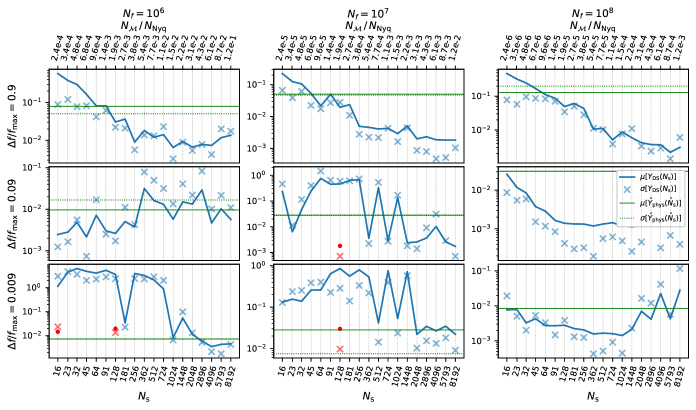
Figure 2: The means and standard deviations of the sets of CMJS divergences, $\overline{D}_{\mathrm{JS}}$, as functions of $N_{\mathrm{s}}$, for the systems presented in Section 4.4.1. The top axis shows the fraction of the signal’s number of Nyquist samples that were required to be computed to evaluate the posteriors. The solid blue line (/blue crosses) shows the CMJS distance mean (/standard deviation) of sets of downsampled posteriors defined using single noise factor, hybrid downsampling, from the target distribution. The solid (/dashed) green lines are the means (/standard deviations) of the posterior noise of zeroed mean distributions defined with physical non-zero noise realisations. The red dots (/crosses) are the means (/standard deviations) of CMJS distances defined using the FIM preservation downsampling method. Convergence criteria is given in Section 4.3, and Table 4.6.2 gives $N_{\mathrm{s}}^{\mathrm{opt}}$ for each system.

 

In Figure 2 and Table 4.6.2, we see that the behaviour of the downsampling for all $\Delta f/f_{\mathrm{max}}=0.9$ systems is as expected, and independent of $N_{\mathrm{f}}$. The other results are far more erratic with no discernible pattern, however, on inspection of the posteriors and consideration of the signal model and downsampling process, an explanation emerges and an important aspect of downsampling is highlighted.

On examining the FIMs of the posteriors that are very divergent from the target distributions, which cause the high degree of posterior noise, we find that they generally have in common that the information on the effective spin parameter far exceeds what should be expected, proportionately, with respect to the other parameters. Less generally, other effects are apparent on comparing the posteriors and the FIMs, such as relative information on certain pairs of parameters being disproportionately represented. Some of these subtle effects are compounded by the non-white noise covariance matrix and become very difficult to disentangle and investigate. However, since the FIM is the main moment of the distribution describing its morphology, ensuring the Fisher information is preserved after downsampling seems to be a possible approach to achieving a better downsampling rate for these extreme cases.

To test this hypothesis, we computed specific sets of posteriors, 21 in each set, for those systems that converged much later than expected. We used the FIM preservation method rather than single factor noise reduction, since this method is of course intended to provide accurate covariances. The means and standard deviations of the particular sets we computed are shown as the red dots (means) and crosses (standard deviations) in Figure 2, and indeed very strongly support this hypothesis. Note that for $N_{\mathrm{f}}=10^{6},\Delta f/f_{\mathrm{max}}=0.009$ we used random rather than hybrid sampling, since dolfen had difficulty finding a solution for FIM preservation in the hybrid case.

This appears to demonstrate that we initially chose a fiducial system with which to determine the optimal downsampling scheme and method in Part 1 that was sub-optimal, and which ultimately has led to the wrong choice of downsampling scheme with which to determine the optimal number of samples. Clearly using FIM preservation allows $N_{\mathrm{s}}^{\mathrm{opt}}\leq 128$ for those systems requiring $N_{\mathrm{s}}^{\mathrm{opt}}\geq 1024$ under single factor downsampling. Replacing the values in the red cells of Table 4.6.2 with the new values, $N_{\mathrm{s}}=128$, we can conclude that, using FIM preservation downsampling, the optimal downsampling number of samples for our range of tested systems is at most $N_{\mathrm{s}}^{\mathrm{opt}}=362$. In many cases it is much smaller than this, however, a method of computing $N_{\mathrm{s}}^{\mathrm{opt}}$ for a specific system (without producing and studying many posteriors as we have done) from, say, the Fisher matrix, presently does not appear to be possible.

5 Speed comparison and further remarks

5.1 Posterior estimate evaluation times

The average PE convergence time for each of the $\Delta f/f_{\mathrm{max}}=0.9$ systems is plotted in Figure 5.1. As to be expected, the evaluation time drops as the number of datapoints is dropped. However, the times reach a minimum of a few hours at around $N_{\mathrm{s}}\approx 256$, then start to rise as $N_{\mathrm{s}}$ continues to drop. The reason for this increase is because the posterior structure begins to qualitatively break down, as extra modes are introduced and the general posterior structure becomes highly irregular, since the low number of datapoints cannot accurately encode the original posterior. The sampler therefore has significantly more difficulty in finding the isoprobability contours, and thus requires more time to converge, despite only computing a small number of datapoint values to evaluate the likelihood.

Figure 3: The average convergence times for selected BHB systems. The relationship is strongly linear after $N_{\mathrm{s}}\gtrsim 362$ since the posterior has stabilised and takes its simplest form; for $N_{\mathrm{s}}\lesssim 128$, posterior estimation time increases as the number of samples decreases, since the structure of the posterior begins to break down, becoming highly irregular and multi-modal, and more difficult for the sampler to explore.

Increasing $N_{\mathrm{s}}$ beyond $N_{\mathrm{s}}^{\mathrm{opt}}$ only increases the amount of time-series datapoint computations required to evaluate the likelihood, without affecting the likelihood (by definition), thus the posterior evaluation time is expected to increase roughly linearly with increasing $N_{\mathrm{s}}$. We see in Figure 5.1 that this is indeed the case, where a line of best fit is drawn through those average times for which $N_{\mathrm{s}}\geq N_{\mathrm{s}}^{\mathrm{opt}}$. Write the linear average PE time as

$$T(N) =aN+c$$ (48a)

and for $$N_{\mathrm{s}}\ll N_{\mathrm{f}}$$,

$$T(N_{\mathrm{s}}) \equiv b(2\mathcal{M}+1)N_{\mathrm{s}}+c\approx bN_{\mathcal{M}}(N_{\mathrm{s}})+c\,,$$ (48b)

using (12), where we have that

$$b =a(2\mathcal{M}+1)^{-1}\,,$$ (48c)

where $T$ is the average evaluation time, $a$ is the line’s gradient and $c$ is a constant time offset that is attributed to the ‘overheads’ of the sampler (internal processes such as initialisation, computing the Fisher matrix, normalising flow transformations carried out by Nessai, etc.).

The linear model of posterior evaluation time can be used to estimate the time it would take to evaluate the posterior using all the samples (when $N_{\mathcal{M}}=N_{\mathrm{Nyq}}$) from which we can roughly gauge the amount of time saved by employing our downsampling procedure. Simulated analyses of LISA data are often done in the frequency domain because of the great simplicity of computing the inner product that is afforded by the independence of the data samples there. The comparison of evaluation times shall not be especially precise because of this (the number of numerical operations required to compute signal templates will differ slightly between time domain and frequency domain signal models). Furthermore, the time domain analysis we have undertaken here requires a few more simple mathematical operations (see Section 3.1.3) in the form of element-wise products. It is reasonable to assume the cost of these operations are quite negligible in relation to the cost of evaluating the signal at the required points however, and particularly if one were to use more realistic GW signal models defined more precisely, consisting of many more terms in the expression of the strain model, $h(t)$. With these caveats mentioned, we can see the linear PE evaluation time parameters in Table 3, along with the comparison between the expected evaluation time of the original posterior with the downsampled posterior. Note that in Table 3 we have

$$\Delta T\equiv T-c\,,$$ (49)

so that, as well as comparing the estimated evaluation times of the original and downsampled posteriors (minus overheads) which of course is of primary interest, we can also see that the quotient is simply given by

$$\frac{\Delta T(N_{1})}{\Delta T(N_{2})}=\frac{aN_{1}}{aN_{2}}=\frac{N_{1}}{N_{2}}\,,$$ (50)

independent of the slope. The fraction of the estimated time of convergence of the original posterior (minus overheads) required for convergence of approximation by downsampling is $N_{\mathcal{M}}(N_{\mathrm{s}}^{\mathrm{opt}})/N_{\mathrm{f}}$.

 

$N_{\mathrm{f}}$	$\Delta f/f_{\mathrm{max}}$	$a$	$b$	$c$	$\Delta T_{N_{\mathrm{f}}}$	$\Delta T_{N_{\mathrm{s}}^{\mathrm{opt}}}$	$\Delta T_{N_{\mathrm{f}}}/\Delta T_{N_{\mathrm{s}}^{\mathrm{opt}}}$
$10^{6}$	0.009	$2.28\times 10^{-3}$	$1.52\times 10^{-4}$	3.10	$1.5\times 10^{2}$	0.82	$1.84\times 10^{2}$
$10^{6}$	0.09	$6.18\times 10^{-3}$	$4.12\times 10^{-4}$	4.38	$4.1\times 10^{2}$	2.24	$1.84\times 10^{2}$
$10^{6}$	0.9	$1.40\times 10^{-3}$	$9.31\times 10^{-5}$	1.05	$9.3\times 10^{1}$	0.51	$1.84\times 10^{2}$
$10^{7}$	0.009	$4.69\times 10^{-3}$	$3.13\times 10^{-4}$	5.50	$3.1\times 10^{3}$	1.70	$1.84\times 10^{3}$
$10^{7}$	0.09	$4.30\times 10^{-3}$	$2.86\times 10^{-4}$	20.46	$2.9\times 10^{3}$	1.56	$1.84\times 10^{3}$
$10^{7}$	0.9	$2.40\times 10^{-3}$	$1.60\times 10^{-4}$	3.21	$1.6\times 10^{3}$	0.87	$1.84\times 10^{3}$
$10^{8}$	0.009	$6.43\times 10^{-3}$	$4.29\times 10^{-4}$	5.50	$4.3\times 10^{4}$	2.33	$1.84\times 10^{4}$
$10^{8}$	0.09	$4.51\times 10^{-3}$	$3.01\times 10^{-4}$	15.46	$3.0\times 10^{4}$	1.63	$1.84\times 10^{4}$
$10^{8}$	0.9	$3.99\times 10^{-3}$	$2.66\times 10^{-4}$	7.14	$2.7\times 10^{4}$	1.45	$1.84\times 10^{4}$

Table 3: Details of the linear best fit model of posterior evaluation times. The parameters $a,b,c$, are from Equations (48). Also shown is the estimated original posterior evaluation time minus the overhead time, $c$, (hours), $\Delta T_{N_{\mathrm{f}}}=\Delta T(N=N_{\mathrm{f}})$ as defined in Equation (49), the average downsampled posterior (using $N_{\mathrm{s}}^{\mathrm{opt}}\!=\!362$) evaluation time minus the overhead time (hours), $\Delta T_{N_{\mathrm{s}}^{\mathrm{opt}}}=\Delta T(N=362)$ and finally the ratio of these times (this is the approximate time saving factor of the posterior evaluation time, after disregarding the constant overheads). Recall these values are computed by setting $\mathcal{M}=7$ for all systems, the highest $\mathcal{M}$ of all systems. Most systems had $\mathcal{M}=4$, however, where $\Delta T_{N_{\mathrm{s}}}$ would be $\tfrac{3}{5}$ of the value given here, had we not manually set $\mathcal{M}=7$.

 

5.2 Discussion

As we can see from the rightmost column of Table 3, the reduction in evaluation times is very large. These times are computed using $N_{\mathrm{s}}=362$ and $\mathcal{M}=7$. For some systems, convergence was achieved in as little as 16 samples, and with true MCS $\mathcal{M}=4$. Recalculating by using these values for the $N_{\mathrm{f}}=10^{8}$ systems we find that $\Delta T_{N_{\mathrm{f}}}/\Delta T_{N_{\mathrm{s}}^{\mathrm{opt}}}=1841.62\to 694444.44$; i.e., likelihood evaluations in this extreme case are computed almost $7\times 10^{5}$ times faster than those of the original, fully sampled datasets would be (this is disregarding the initialisation and sampler overheads). However, most LISA signals will not have as many Nyquist datapoints, and many signals will have $\mathcal{M}>4$. Furthermore, since it is not yet known prior to study of a given PE problem what the optimal downsampling rate for that system is, it is necessary to use a higher number of datapoints to avoid potential misrepresentation of the true posterior; see Section 6.2 for further discussion on proper use of dolfen.

The dimensionality of the signal model has not yet been discussed. The $n$-dimensional posteriors we have studied can be thought of as slices of $(n+1)$-dimensional posteriors. In an $(n+1)$-dimensional PE situation, the likelihood values at points on these $n$-dimensional slices will not be affected simply by allowing likelihood values on neighbouring slices also to be computed. Since there is nothing special about a particular slice, the neighbouring slices can thus be expected to be similarly accurately approximated, and one should be able to build up an accurate $(n+1)$-dimensional posterior using the same, downsampled subset of datapoints, by combining slices. One can continue to add more parameters in this way, and downsampling is not expected to be very strongly dependent on the number of free model parameters. Accuracy must of course be checked by the user for very high numbers of parameters. Some informal tests on 17-dimensional posteriors using $N_{\mathrm{s}}=500$ (default dolfen setting) have shown extremely consistent results, indicating high accuracy up to at least 17-dimensions.

We have suggested and tested various downsampling methods and schemes. After originally coming to the conclusion that hybrid, single factor downsampling was marginally more efficient in Section 4.6.1, we produced large sets of posteriors using this method in Section 5.1. We then discovered the surprising behaviour of some systems as highlighted in Figure 2 and Table 4.6.2, and recognised potential model dependent causes that might be remedied by using the FIM preservation method. A clue that FIM preservation is the more effective method was present in Figure 4.6.1, and was unfortunately missed: in that figure we can see general agreement between all methods and schemes, apart from the cluster scheme. This performed badly with single factor, but vastly improved with FIM preservation; given a datapoint subset that poorly represent the posterior under single factor modification, vast improvements can be made using FIM preservation instead. The FIM preservation statistics for a few test systems were computed and shown as the red marks in Figure 4.6.1, which at $N_{\mathrm{s}}=128$ are already approximately equal to the statistics of the converged posteriors under single factor noise reduction ($N_{\mathrm{s}}\gtrsim 1448$).

It has been demonstrated here that downsampling is a viable approach for cheaply and accurately reproducing the likelihood function in simulated environments. However, unfortunately no means of determining $N_{\mathrm{s}}^{\mathrm{opt}}$ for a given PE problem appears to be derivable from simpler objects, such as the FIM, from within the standard PE framework. For readers familiar with machine learning techniques, one can think of the downsampled data space as being akin to the so-called latent space that is often used as a low-dimensional space of auxiliary coordinates, which represents and stands in for high-dimensional data. The map from the latent space variables to the appropriate representation of the high-dimensional data is ‘learned’ by the machine learning algorithms. Downsampling seeks generality, and to skip the map learning part, by using restrictions of its ‘latent space’ (the downsampled data space) map provided by the signal model, and optimisations of that map by the downsampling methods detailed in this paper. We also mentioned that a helpful way to think of downsampling is by considering the signal and noise model at the remaining data points as an encoding scheme for the morphology of the posterior. Without first knowing the posterior however, we do not know what to encode. Downsampling is fundamentally limited by these problems, and the accuracy of a posterior can never be guaranteed, however, using the FIM preservation method over minimising Jeffreys’ divergences of the PCMs has provided a much improved and highly accurate result for our example systems. For many applications, the default settings of the downsampling software will likely yield accurate results, and should most certainly be acceptable for making informal research enquiries. However, in the absence of a guarantee of accuracy, when a user wishes to show certainty that a downsampled posterior is very highly accurate (say, for publication), it should be ensured that convergence has been reached by producing a number of posteriors at different $N_{\mathrm{s}}$ and comparing these, to show that the posteriors are independent of $N_{\mathrm{s}}$.

Whilst we have seen vast improvement in PE evaluation times, many realistic signal models will be more intricate than our standard BBH inspiral signal, with likelihood functions that are generally more costly to compute. The approximation techniques like the one expounded here, and others, such as ROQ, become essential tools for experimentation in the PE environment with LISA-like signals that are prohibitively expensive to compute. As shown in the $c$ & $\Delta T_{N_{\mathrm{s}}^{\mathrm{opt}}}$ columns of Table 3, the PE evaluation time for our test systems can be mostly attributed to initialisation and the internal workings of the sampler. But it is easy to envisage that, for very expensive models, which may also require using higher $N_{\mathrm{s}}$ depending on their slow evolution status, the likelihood evaluation time may again become the primary factor. Amongst possible future steps is the investigation of whether and how the different mentioned approximation techniques can be combined, to produce an even more rapid feedback arena for studying BHB signals and their various waveform modifications in LISA.

6 The dolfen package

The downsampling likelihood function estimation package: dolfen, performs all variants of the downsampling procedure that have been derived and discussed in this article. dolfen is a pip installable python package that can easily be used in conjunction with bilby [27] as per the examples provided on dolfen’s documentation pages (https://dolfen.readthedocs.io) and github pages (https://github.com/jethrolinley/dolfen).

6.1 Future developments

Recall from Section 3.4 that numerical issues often arise in exact FIM preservation. Approximate FIM preservation is far easier to solve, and dolfen appears to succeed most often in implementing this technique. In a subsequent version of dolfen, we intend to include another FIM preservation method; rather than find an individual sample reweighting solution for (approximate) FIM preservation in a given basis (see equation (26)), we shall simply use some (pre-existing) optimisation method to find individual datapoint reweightings (strictly positive) that minimises divergence between the FIMs.

6.2 Recommended usage

In order to conclusively state that a posterior approximation is close to the original posterior one is trying to estimate, the original posterior must already be known so they can be compared. Of course if one has the original, then one doesn’t need an approximation. Downsampling makes an educated guess at how best to optimise the encoding scheme provided by the random sample selection, which then can be thought of as giving a lossy compression of the likelihood. Therefore (although accuracy is likely) there are no guarantees that the likelihood returned will be accurate; the user must be responsible for this. In dolfen, one can set $N_{\mathrm{s}}$, and override the computed MCS, $\mathcal{M}$. So to begin, set, say, $N_{\mathrm{s}}=100$, and $\mathcal{M}=0$. The likelihood should not be expected to be accurate, but one can quickly get a good idea of the general likelihood morphology, to set priors and sampler settings, and so on. Once one has a rough idea of the posterior from these settings, we can use dolfen with its default settings to obtain a likely accurate likelihood. Produce a few, say 3, posteriors with different random datapoint selections (with a zero noise realisation) to confirm convergence. It is very unlikely that multiple poor representations will yield the same or similar posterior by chance, so if the posteriors are similar, convergence is clearly demonstrated. Otherwise, the number of datapoints should be increased.

7 Acknowledgements

The author is grateful to Graham Woan and John Veitch for many helpful discussions, and to Michael Williams, for help in operating his sampler Nessai. This work was partly funded by STFC grant ST/S505390/1. We are grateful for computational resources provided by Cardiff University, and funded by an STFC grant supporting UK Involvement in the Operation of Advanced LIGO. Software: dolfen is implemented in python and uses NumPy [28] and SciPy [29].

Appendix A Other required preliminary results

A.1 Noise covariance matrix introduction

The noise power generated by the detector as a function of frequency (the PSD) determines the degree to which any two samples in the time domain representation of the noise are correlated with each other. In the current section and the next, we derive the time-domain inner product operator (the matrix $\mathbf{C}^{-1}$) from the PSD to account for this interdependence of the samples. It will be assumed that the noise is wide sense stationary (WSS), that is, that its mean and covariance are time invariant.

A cross-covariance matrix of two vectors describes the covariance between elements of the vectors. The $i,j$ element of the cross-covariance matrix $\mathbf{C}_{\mathbf{XY}}$ is the covariance between the $i^{\mathrm{th}}$ element of $\mathbf{X}$ and the $j^{\mathrm{th}}$ element of $\mathbf{Y}$. A cross-covariance matrix is called an auto-covariance, or simply covariance matrix when describing the covariance between different elements of the same vector. Our noise covariance matrix will be denoted in shorthand here as $\mathbf{C}$, so that

$$\mathbf{C}\equiv\mathbf{C}_{\mathbf{nn}}\,,$$ (51)

where $\mathbf{n}$ is a noise realisation. In terms of matrix elements, we define a cross-covariance matrix as

$$C_{ij}\equiv\mathrm{cov}[X_{i},Y_{j}]=\mathbb{E}[(X_{i}-\mathbb{E}[X_{i}])(Y_{j}-\mathbb{E}[Y_{j}])]\,,$$ (52)

where $\mathbb{E}$ is the expectation value operator. For vanishing mean of the noise, we have

$$C_{ij}=\mathbb{E}[n_{i}n_{j}]\equiv R_{ij}\,,$$ (53)

defining the autocorrelation matrix, $R_{ij}$. Now since the noise is assumed to be WSS, the expected value of the product of any two samples only depends on the time ‘lag’ between the samples, i.e., $\mathbb{E}[n_{i}n_{j}]\!=\!\mathbb{E}[n_{i+c}n_{j+c}]$ for any integer $c$. It will be useful to consider $c=-i$ where we have that

$$R_{ij}=\mathbb{E}[n_{i-i}n_{j-i}]=\mathbb{E}[n_{0}n_{j-i}]\,.$$ (54)

In this form, we can see the matrix is both symmetric and circulant. It is clear that the $i,j$ element represents the expected value of noise correlations of time series samples separated by the absolute time lag between the $i^{\mathrm{th}}$ and $j^{\mathrm{th}}$ sample. The first row, $R_{0i}=\mathbb{E}[n_{0}n_{i}]$, gives precisely the definition of the (discrete) ACF.

By the Wiener-Khinchin theorem, the ACF is the Fourier Transform of the PSD. However, we must be careful in the GW data analysis world since, again, we most often use the one-sided PSD which introduces a factor of 2, such that the equation embodying the Wiener-Khinchin theorem reads

$$S_{\mathrm{n}}(f)=2\int_{-\infty}^{\infty}\mathrm{d}t\,R(t)e^{-2\pi ift}=2\,\mathcal{F}\{R\}(f)\,.$$ (55)

Thus given the PSD we can easily compute $\mathbf{C}$, since it is defined by $R_{ij}=R(t_{i}-t_{j})$. For the inner product however, we require $\mathbf{C}^{-1}$. When $N\!=\!\dim(\mathbf{d})$ becomes large, numerical inversion of the resulting $N\times N$ noise covariance matrix becomes very unwieldy. We have devised a fast and accurate solution to this problem, which we now describe.

A.2 Fast inversion of very large autocorrelation matrices

We wish to find the matrix $\mathbf{C}^{-1}$ that satisfies $\mathbf{C}\mathbf{C}^{-1}\!=\!\mathds{1}$, where $\mathbf{C}$ is the noise covariance matrix described in the previous section. Since $\mathbf{C}$ is circulant, it follows that $\mathbf{C}^{-1}$ is circulant also. Then, in components, we can transform indices thus

$$\mathds{1}_{ik}=C_{ij}C^{-1}_{jk}\longrightarrow\mathds{1}_{i^{\prime}0}=C_{i^{\prime}j^{\prime}}C^{-1}_{j^{\prime}0}=R_{i^{\prime}j^{\prime}}R^{-1}_{j^{\prime}0}\,,$$ (56)

where summation over $j$ is implied by the repeated indices, and where we defined $i^{\prime}=(i-k)_{\mod N}$ and $j^{\prime}=(j-k)_{\mod N}$. Dropping primes and using the circulant property of $R_{ij}$:

$$\mathds{1}_{i0}=R_{ij}R^{-1}_{j0}=R_{k0}R^{-1}_{j0}\,,$$ (57)

where now $k=(i-j)_{\mod N}$. It is clear that the problem is reduced to a set of sums over only the first column from each matrix. For these column vectors, we shall use the notation $R[i]\equiv R_{i0}$, and $R^{-1}[i]\equiv R^{-1}_{i0}$. Explicitly writing the sum over $j$ from (57):

$$\mathds{1}_{i0}=\sum_{j=0}^{N-1}R[(i-j)_{\mod N}]R^{-1}[j]\,.$$ (58)

The vector, or discrete function $R$, is the ACF, known by the Wiener-Khinchin theorem, and where $R^{-1}$ is the (discrete) function we seek, which we call the inverse autocorrelation function.

This sum is precisely the form of a circular convolution modulo $N$ ($*_{N}$ operator) of $R$ with $R^{-1}$, so we can write

$$\mathds{1}_{i0}=(R*_{N}R^{-1})[i]\,.$$ (59)

If $\mathcal{F}$ denotes the Fourier Transform and $\mathcal{F}^{-1}$ its inverse, then the convolution theorem states that

$$\mathcal{F}\{R*_{N}R^{-1}\}=\mathcal{F}\{R\}\cdot\mathcal{F}\{R^{-1}\}\,,$$ (60)

so that after Fourier transforming (59), using the convolution theorem, and some rearranging, we get

$$R^{-1}[j] =\mathcal{F}^{-1}\left\{\bigg{(}\mathcal{F}\{R\}\bigg{)}^{-1}\right\}[j]=\mathcal{F}^{-1}\left\{\left(\tfrac{1}{2}S_{\mathrm{n}}\right)^{-1}\right\}[j]\,,$$ (61)

where we substituted for the PSD from (55). The discrete $R^{-1}$ is the first row of $\mathbf{C}^{-1}$, which defines the whole matrix $\mathbf{C}^{-1}$, since we know it is circulant.

A.3 Whitening transformation matrix

We will require an operator to transform vectors of correlated datapoints to vectors of uncorrelated datapoints. Suppose a noise weighted (time domain) inner product of signals can be represented in another basis in which the datapoints are uncorrelated from each other. The inner product matrix in such a basis is diagonal. Further, suppose the basis vectors are scaled such that this matrix is the identity matrix. Since inner products are invariant under basis transformations, we can define a transformed inner product of vectors $\mathbf{a}$ and $\mathbf{b}$ by

$$\mathbf{a}^{\mathrm{\scriptscriptstyle T}}\mathbf{C}^{-1}\mathbf{b}=\mathbf{\bar{a}}^{\mathrm{\scriptscriptstyle T}}\mathds{1}\;\mathbf{\bar{b}}\,,$$ (62)

for general time domain inner product matrix $\mathbf{C}^{-1}$, and where $\mathbf{\bar{a}}$ and $\mathbf{\bar{b}}$ are the ‘whitened’ representations of vectors $\mathbf{a}$ and $\mathbf{b}$. We shall solve this here by writing

$$\mathbf{a}^{\mathrm{\scriptscriptstyle T}}\mathbf{C}^{-1}\mathbf{b} =\mathbf{a}^{\mathrm{\scriptscriptstyle T}}\mathbf{C}^{(-1/2)}\mathbf{C}^{(-1/2)}\mathbf{b}$$

$$=\mathbf{a}^{\mathrm{\scriptscriptstyle T}}\left(\mathbf{C}^{(-1/2)}\right)^{\mathrm{\scriptscriptstyle T}}\mathds{1}\mathbf{C}^{(-1/2)}\mathbf{b}\,,$$ (63)

where $\mathbf{C}^{(-1/2)}$ is some matrix to be found, which we shall constrain to be symmetric circulant (since $\mathbf{C}^{(-1)}$ is symmetric circulant, and a product of circulant matrices is circulant). We can then read off the whitening transformation of the vector space, in which $\mathbf{C}^{-1}\to\mathds{1}$ along with all vectors $\mathbf{v}\to\bar{\mathbf{v}}=\mathbf{C}^{(-1/2)}\mathbf{v}$. Noting that

$$\mathbf{C}^{-1}=\mathbf{C}^{(-1/2)}\mathbf{C}^{(-1/2)}\,,$$ (64)

we make use of the circulant properties to write this in components as

$$C^{-1}_{ik}=C^{(-1/2)}_{ij}C^{(-1/2)}_{jk}\longrightarrow C^{-1}_{i^{\prime}0}=C^{(-1/2)}_{i^{\prime}j^{\prime}}C^{(-1/2)}_{j^{\prime}0}\,,$$ (65)

where again we define $i^{\prime}=(i-k)_{\mod N}$ and $j^{\prime}=(j-k)_{\mod N}$. Dropping primes and using the circulant property of $\mathbf{C}^{(-1/2)}$:

$$C^{-1}_{i0}=C^{(-1/2)}_{k0}C^{(-1/2)}_{j0}\,,$$ (66)

where again we have now defined $k=(i-j)_{\mod N}$. We are now dealing with single columns of the matrices, and write these vectors as $C^{-1}[i]=C^{-1}_{i0}$, and $C^{(-1/2)}[i]=C^{(-1/2)}_{i0}$. Writing the sum in equation (66) explicitly:

$$C^{-1}[i] =\sum_{j=0}^{N-1}C^{(-1/2)}[(i-j)_{\mod N}]C^{(-1/2)}[j]$$

$$=\left(C^{(-1/2)}*_{N}C^{(-1/2)}\right)[i]\,,$$

where $C^{-1}=R^{-1}$ is the inverse auto-correlation function we defined earlier in equation (61), and $C^{(-1/2)}$ shall be referred to either as the whitening function or decorrelation function and is the function sought. Fourier transforming gives

$$\mathcal{F}\{C^{-1}\}=\bigg{[}\mathcal{F}\{C^{(-1/2)}\}\bigg{]}^{2}\,,$$ (67)

so that

$$C^{(-1/2)}=\mathcal{F}^{-1}\left\{\sqrt{\mathcal{F}\{C^{-1}\}}\right\}\,.$$ (68)

However, we know that $\mathcal{F}\{C^{-1}\}=2/S_{\mathrm{n}}$, as in equation (61) for example, so we finally write the whitening function as

$$C^{(-1/2)}=\mathcal{F}^{-1}\left\{\sqrt{2/S_{\mathrm{n}}}\right\}\,,$$ (69)

where the matrix version $C^{(-1/2)}_{ij}\equiv C^{(-1/2)}(t_{i}-t_{j})$; this is the whitening matrix, or decorrelation matrix. From (53) and (64) we can then write

$$R^{-1}_{ik}=R^{(-1/2)}_{ij}R^{(-1/2)}_{jk}$$ (70)

which is the first column of, and thus defines, since it is circulant, the whitening matrix, or decorrelation matrix, $C^{(-1/2)}_{ij}=R^{(-1/2)}_{ij}$.

Appendix B Minimising the Jeffreys’ Divergence of Gaussians

Let $\Theta$ be the space of parameters $\bm{\theta}$, with dimension $k=\mathrm{dim}(\Theta)$. Let $(\mathcal{D}_{\mathrm{f}},\mathbb{C}_{\mathrm{f}}^{-1})$ be the data space and inner product operator pair for the full dataset (subscript _f). If the posterior defined on the parameter space, $p_{\mathrm{f}}(\bm{\theta})$, is Gaussian, it can be written

$$p_{\mathrm{f}}(\bm{\theta})=\left[(2\pi)^{k}|\mathbf{F}_{\mathrm{f}}^{-1}|\right]^{-1/2}\exp\left[-\tfrac{1}{2}\bm{\Delta}^{\mathrm{\scriptscriptstyle T}}\mathbf{F}_{\mathrm{f}}\bm{\Delta}\right]\,,$$ (71)

where $\mathbf{F}_{\mathrm{f}}$ is the FIM of the full dataset, $|\mathbf{F}_{\mathrm{f}}^{-1}|$ is the determinant of its inverse, $\bm{\Delta}\equiv\bm{\theta}-\bm{\hat{\theta}}$ and $\bm{\hat{\theta}}$ is the location of the peak of the posterior. Suppose there also exists the space $(\mathcal{D}_{\mathrm{s}},\mathbf{M})$, with the posterior $p^{\prime}_{\mathrm{s}}(\bm{\theta})$, and where $\mathbf{F}^{\prime}_{\mathrm{s}}$ is the FIM in $(\mathcal{D}_{\mathrm{s}},\mathbf{M})$, where $\mathbf{M}$ is some Ansatz matrix (we will set this equal to $\mathds{1}$ so that each sample is weighted equally). This is the (unmodified) downsampled subspace, that is: $\mathcal{D}_{\mathrm{s}}\subset\mathcal{D}_{\mathrm{f}}$.

Finally, let $(\mathcal{D}_{\mathrm{s}},\mathbb{C}_{\mathrm{s}}^{-1}\!=\!m\mathbf{M})$ be a data space and inner product operator pair for a downsampled dataset, where $m$ is the constant we seek. Write the Gaussian posterior similarly on this pair, $p_{\mathrm{s}}(\bm{\theta})$, as

$$p_{\mathrm{s}}(\bm{\theta})=\left[(2\pi)^{k}|\mathbf{F}_{\mathrm{s}}^{-1}|\right]^{-1/2}\exp\left[-\tfrac{1}{2}\bm{\Delta}^{\mathrm{\scriptscriptstyle T}}\mathbf{F}_{\mathrm{s}}\bm{\Delta}\right]\,,$$ (72)

where $\mathbf{F}_{\mathrm{s}}$ is the FIM of the downsampled dataset.

Ideally, we would minimise the JS divergence, since this is a well-known, symmetric measure of distance between distributions and is impartial to either distribution, unlike the KL divergence, which implies its first argument is the true distribution and its second is a sample distribution. However, we are choosing our posterior to be a replacement for the truth, not some sample distribution with minimal divergence from it, so we require a symmetric divergence measure. The JS divergence is defined in equation (4.2). It contains the integral of the log of a sum and only special cases are able to be integrated analytically. In order to avoid prioritisation of any given distribution, we shall attempt to minimise another symmetric divergence known as the Jeffreys’-divergence instead, simply defined by

$$D_{\mathrm{J}}\Big{(}p_{\mathrm{f}}\,\Big{|}\Big{|}\,p_{\mathrm{s}}\Big{)}\equiv D_{\mathrm{KL}}\Big{(}p_{\mathrm{f}}\,\Big{|}\Big{|}\,p_{\mathrm{s}}\Big{)}+(p_{\mathrm{s}}\leftrightarrow p_{\mathrm{f}})\,.$$ (73)

First however, we warm up by minimising the KL divergence, before moving on to the Jeffreys’ divergence.

We have the unknown $m$ in $(\mathcal{D}_{\mathrm{s}},\mathbb{C}_{\mathrm{s}}^{-1})$, but $(\mathcal{D}_{\mathrm{s}},\mathbf{M})$ and $(\mathcal{D}_{\mathrm{f}},\mathbb{C}_{\mathrm{f}}^{-1})$ are known completely. Using the Gaussian approximations, we write down the KL divergence to find the $m$ that minimises the KL divergence between $p_{\mathrm{s}}(\bm{\theta})$ and $p_{\mathrm{f}}(\bm{\theta})$:

$$D_{\mathrm{KL}}(p_{\mathrm{f}}(\bm{\theta})\,||\,p_{\mathrm{s}}(\bm{\theta}))\equiv \int_{\Theta}\mathrm{d}^{k}\theta\,p_{\mathrm{f}}(\bm{\theta})\ln\left(\frac{p_{\mathrm{f}}(\bm{\theta})}{p_{\mathrm{s}}(\bm{\theta})}\right)$$

$$= \int_{\Theta}\mathrm{d}^{k}\theta\,p_{\mathrm{f}}(\bm{\theta})\left[\ln\left(\sqrt{\frac{|{\mathbf{F}_{\mathrm{s}}}^{-1}|}{|\mathbf{F}_{\mathrm{f}}^{-1}|}}\right)+\tfrac{1}{2}\bm{\Delta}^{\mathrm{\scriptscriptstyle T}}(\mathbf{F}_{\mathrm{s}}-\mathbf{F}_{\mathrm{f}})\bm{\Delta}\right]$$

$$= \ln\left(m^{-k/2}\sqrt{\frac{|{\mathbf{F}^{\prime}}_{\mathrm{s}}^{-1}|}{|\mathbf{F}_{\mathrm{f}}^{-1}|}}\right)+\tfrac{1}{2}\int_{\Theta}\mathrm{d}^{k}\theta\,p_{\mathrm{f}}(\bm{\theta})\cdot\bm{\Delta}^{\mathrm{\scriptscriptstyle T}}(m\mathbf{F}^{\prime}_{\mathrm{s}}-\mathbf{F}_{\mathrm{f}})\bm{\Delta}\,,$$ (74)

since the integral of the posterior (which we take to be normalised) over parameter space is equal to 1. In the last line, we also used the definition of the FIM in equation (15) and $\mathbb{C}_{\mathrm{s}}^{-1}\!=\!m\mathbf{M}$ to find that

$$F_{\mathrm{s},ij}=h_{k,i}(\mathbb{C}_{\mathrm{s}}^{-1})_{kl}h_{l,j}=mh_{k,i}M_{kl}h_{l,j}=mF^{\prime}_{\mathrm{s},ij}\,,$$ (75)

or $\mathbf{F}_{\mathrm{s}}=m\mathbf{F}^{\prime}_{\mathrm{s}}$, from which we obtain

$$|\mathbf{F}_{\mathrm{s}}|=m^{k}|\mathbf{F}^{\prime}_{\mathrm{s}}|\,.$$ (76)

The KL divergence is a function of $m$, with the minimum being the $m$ at which the derivative with respect to $m$ vanishes (it is clear, given our restriction to considering Gaussians, that there will always be one extremum only, which is a minimum). The minimum is given by the $m=m_{\mathrm{KL}}$ solving $\frac{\mathrm{d}}{\mathrm{d}m}D_{\mathrm{KL}}(p_{\mathrm{f}}(\bm{\theta})\,||\,p_{\mathrm{s}}(\bm{\theta}))=0$, which is

$$m_{\mathrm{KL}} =k\left(\int_{\Theta}\mathrm{d}^{k}\theta\,p_{\mathrm{f}}(\bm{\theta})\cdot\bm{\Delta}^{\mathrm{\scriptscriptstyle T}}\mathbf{F}^{\prime}_{\mathrm{s}}\bm{\Delta}\right)^{-1}\,.$$ (77)

To compute the integral, let us change coordinates first by a translation $\theta_{\mu}\to{\theta}^{\star}_{\mu}$ that takes $\bm{\hat{\theta}}\to{\bm{\hat{\theta}}}^{\star}=\mathbf{0}$, centering the peak of the posterior at the origin, so that $\bm{\Delta}\to{\bm{\Delta}}^{\star}={\bm{\theta}}^{\star}$. Then perform a rotation ${\theta}^{\star}_{\mu}\to\widetilde{\theta}_{\mu}$ such that $\mathbf{F}_{\mathrm{f}}^{\star}\to\widetilde{\mathbf{F}}_{\mathrm{f}}$, where the matrix $\widetilde{\mathbf{F}}_{\mathrm{f}}$ is diagonal, i.e., aligning the coordinate axes with the ellipsoid axes. We denote all objects in the final coordinates with a tilde accent. Both transformations are unitary resulting in a Jacobian determinant equal to 1, and if we further suppose that $\bm{\Theta}\sim\mathbb{R}^{k}$ then also $\widetilde{\bm{\Theta}}\sim\mathbb{R}^{k}$, so we can write the integral in (77) as

$$\int_{\Theta}\mathrm{d}^{k}\theta\,p_{\mathrm{f}}(\bm{\theta})\cdot\bm{\Delta}^{\mathrm{\scriptscriptstyle T}}\mathbf{F}^{\prime}_{\mathrm{s}}\bm{\Delta} =\int_{\widetilde{\Theta}}\mathrm{d}^{k}\widetilde{\theta}\,p_{\mathrm{f}}(\widetilde{\bm{\theta}})\cdot\widetilde{\bm{\theta}}^{\mathrm{\scriptscriptstyle T}}\widetilde{\mathbf{F}}^{\prime}_{\mathrm{s}}\widetilde{\bm{\theta}}$$

$$=\left[(2\pi)^{k}\left|\widetilde{\mathbf{F}}_{\mathrm{f}}^{-1}\right|\right]^{-1/2}\int_{\widetilde{\Theta}}\mathrm{d}^{k}\widetilde{\theta}\,\exp\left[-\tfrac{1}{2}\widetilde{\bm{\theta}}^{\mathrm{\scriptscriptstyle T}}\widetilde{\mathbf{F}}_{\mathrm{f}}\widetilde{\bm{\theta}}\right]\cdot\widetilde{\bm{\theta}}^{\mathrm{\scriptscriptstyle T}}\widetilde{\mathbf{F}}^{\prime}_{\mathrm{s}}\widetilde{\bm{\theta}}$$

$$=\left[(2\pi)^{k}\left|\widetilde{\mathbf{F}}_{\mathrm{f}}^{-1}\right|\right]^{-1/2}\int_{\widetilde{\Theta}}\mathrm{d}^{k}\widetilde{\theta}\,\exp\left[-\tfrac{1}{2}\sum_{l=1}^{k}\widetilde{F}_{\mathrm{f},ll}\widetilde{\theta}_{l}^{2}\right]\sum_{i,j=1}^{k}\widetilde{\theta}_{i}\widetilde{F}^{\prime}_{\mathrm{s},ij}\widetilde{\theta}_{j}$$

$$=\left[(2\pi)^{k}\left|\widetilde{\mathbf{F}}_{\mathrm{f}}^{-1}\right|\right]^{-1/2}\sum_{i,j=1}^{k}\widetilde{F}^{\prime}_{\mathrm{s},ij}\int_{\widetilde{\Theta}}\mathrm{d}^{k}\widetilde{\theta}\,\prod_{l=1}^{k}\exp\left[-\tfrac{1}{2}\widetilde{F}_{\mathrm{f},ll}\widetilde{\theta}_{l}^{2}\right]\widetilde{\theta}_{i}\widetilde{\theta}_{j}\,.$$

Noting the well-known integral formulas:

$$\int_{-\infty}^{\infty}\mathrm{d}x\;e^{-ax^{2}}=\sqrt{\pi/a}\,,\;\;\;\;\;\;\;\;\;\int_{-\infty}^{\infty}\mathrm{d}x\;x\,e^{-ax^{2}}=0\,,\;\;\;\;\;\;\;\;\;\int_{-\infty}^{\infty}\mathrm{d}x\;x^{2}\,e^{-ax^{2}}=\frac{\sqrt{2\pi}}{(2a)^{3/2}}\,,$$ (78)

we find that the only surviving terms in the $i,j$ sum are the $i=j$ terms. The integral becomes

$$\int_{\Theta}\mathrm{d}^{k}\theta\,p_{\mathrm{f}}(\bm{\theta})\cdot\bm{\Delta}^{\mathrm{\scriptscriptstyle T}}\mathbf{F}^{\prime}_{\mathrm{s}}\bm{\Delta} =\left[(2\pi)^{k}\left|\widetilde{\mathbf{F}}_{\mathrm{f}}^{-1}\right|\right]^{-1/2}\sum_{i=1}^{k}\widetilde{F}^{\prime}_{\mathrm{s},ii}\int_{-\infty}^{\infty}\mathrm{d}\widetilde{\theta}_{i}\,\widetilde{\theta}_{i}^{2}\,e^{-\frac{1}{2}\widetilde{F}_{\mathrm{f},ii}\widetilde{\theta}_{i}^{2}}\prod_{j\neq i}\int_{-\infty}^{\infty}\mathrm{d}\widetilde{\theta}_{j}\,e^{-\frac{1}{2}\widetilde{F}_{\mathrm{f},jj}\widetilde{\theta}_{j}^{2}}$$

$$=\left[(2\pi)^{k}\left|\widetilde{\mathbf{F}}_{\mathrm{f}}^{-1}\right|\right]^{-1/2}\sum_{i=1}^{k}\widetilde{F}^{\prime}_{\mathrm{s},ii}\sqrt{\frac{2\pi}{\widetilde{F}^{3}_{\mathrm{f},ii}}}\;\prod_{j\neq i}\sqrt{\frac{2\pi}{\widetilde{F}_{\mathrm{f},jj}}}$$

$$=\sum_{i=1}^{k}\frac{\widetilde{F}^{\prime}_{\mathrm{s},ii}}{\widetilde{F}_{\mathrm{f},ii}}\,.$$ (79)

If the matrix $\mathbf{G}$ diagonalises $\mathbf{F}_{\mathrm{f}}$, that is, if $\mathbf{F}_{\mathrm{f}}\to\widetilde{\mathbf{F}}_{\mathrm{f}}=\mathbf{G}^{-1}{\mathbf{F}}_{\mathrm{f}}\mathbf{G}$ for diagonal $\widetilde{\mathbf{F}}_{\mathrm{f}}$, then the integral may be written

$$\int_{\Theta}\mathrm{d}^{k}\theta\,p_{\mathrm{f}}(\bm{\theta})\cdot\bm{\Delta}^{\mathrm{\scriptscriptstyle T}}\mathbf{F}^{\prime}_{\mathrm{s}}\bm{\Delta}=\sum_{i=1}^{k}\frac{G^{-1}_{ij}F^{\prime}_{\mathrm{s},jl}G_{li}}{G^{-1}_{ij}F_{\mathrm{f},jl}G_{li}}\,,$$ (80)

or for general symmetric matrices $\mathbf{A}$ and $\mathbf{B}$, and with $\mathbf{P}$ diagonalising $\mathbf{A}$, we have

$$\int_{\Theta}\mathrm{d}^{k}\theta\,e^{-\frac{1}{2}\bm{\Delta}^{\mathrm{\scriptscriptstyle T}}\mathbf{A}\bm{\Delta}}\cdot\bm{\Delta}^{\mathrm{\scriptscriptstyle T}}\mathbf{B}\bm{\Delta}=\sqrt{\frac{(2\pi)^{k}}{|\mathbf{A}|}}\sum_{i=1}^{k}\frac{P^{-1}_{ij}B_{jl}P_{li}}{P^{-1}_{ij}A_{jl}P_{li}}\,.$$ (81)

Therefore our factor $m_{\mathrm{KL}}$, using (77) is

$$m_{\mathrm{KL}} =k\left(\sum_{i=1}^{k}\frac{G^{-1}_{ij}F^{\prime}_{\mathrm{s},jl}G_{li}}{G^{-1}_{ij}F_{\mathrm{f},jl}G_{li}}\right)^{-1}\,.$$ (82)

This in particular minimises $D_{\mathrm{KL}}(p_{\mathrm{f}}\,||\,p_{\mathrm{s}})$, which should be noted is not equal to $D_{\mathrm{KL}}(p_{\mathrm{s}}\,||\,p_{\mathrm{f}})$: the KL divergence not symmetric. Let us now minimise the symmetric Jeffreys’ divergence. With equation (73), this can be written as

$$D_{\mathrm{J}}(p_{\mathrm{f}}\,||\,p_{\mathrm{s}}) \equiv\int_{\Theta}\mathrm{d}^{k}\theta\,(p_{\mathrm{f}}-p_{\mathrm{s}})\cdot\ln\left(\frac{p_{\mathrm{f}}}{p_{\mathrm{s}}}\right)$$

$$=\int_{\Theta}\mathrm{d}^{k}\theta\,(p_{\mathrm{f}}-p_{\mathrm{s}})\left[\ln\left(\sqrt{\frac{|{\mathbf{F}_{\mathrm{s}}}^{-1}|}{|\mathbf{F}_{\mathrm{f}}^{-1}|}}\right)+\tfrac{1}{2}\bm{\Delta}^{\mathrm{\scriptscriptstyle T}}(\mathbf{F}_{\mathrm{s}}-\mathbf{F}_{\mathrm{f}})\bm{\Delta}\right]$$

$$=\tfrac{1}{2}\int_{\Theta}\mathrm{d}^{k}\theta\,(p_{\mathrm{f}}-p_{\mathrm{s}})\cdot\bm{\Delta}^{\mathrm{\scriptscriptstyle T}}(m\mathbf{F}^{\prime}_{\mathrm{s}}-\mathbf{F}_{\mathrm{f}})\bm{\Delta}\,,$$ (83)

again since the integral of both $p_{\mathrm{f}}$ and $p_{\mathrm{s}}$ over the whole space must be equal to 1. Writing out $p_{\mathrm{f}}$ and $p_{\mathrm{s}}$ in full we have

$$D_{\mathrm{J}}(p_{\mathrm{f}}\,||\,p_{\mathrm{s}}) =\tfrac{1}{2}\int_{\Theta}\mathrm{d}^{k}\theta\,\left[\sqrt{\frac{|\mathbf{F}_{\mathrm{f}}|}{(2\pi)^{k}}}e^{-\frac{1}{2}\bm{\Delta}^{\mathrm{\scriptscriptstyle T}}\mathbf{F}_{\mathrm{f}}\bm{\Delta}}-\sqrt{\frac{m^{k}|{\mathbf{F}^{\prime}}_{\mathrm{s}}|}{(2\pi)^{k}}}e^{-\frac{1}{2}m\bm{\Delta}^{\mathrm{\scriptscriptstyle T}}\mathbf{F}^{\prime}_{\mathrm{s}}\bm{\Delta}}\right]\cdot\bm{\Delta}^{\mathrm{\scriptscriptstyle T}}(m\mathbf{F}^{\prime}_{\mathrm{s}}-\mathbf{F}_{\mathrm{f}})\bm{\Delta}$$

$$=C\int_{\Theta}\mathrm{d}^{k}\theta\,\left[C^{\prime}e^{-\frac{1}{2}\bm{\Delta}^{\mathrm{\scriptscriptstyle T}}\mathbf{F}_{\mathrm{f}}\bm{\Delta}}-m^{k/2}e^{-\frac{1}{2}m\bm{\Delta}^{\mathrm{\scriptscriptstyle T}}\mathbf{F}^{\prime}_{\mathrm{s}}\bm{\Delta}}\right]\cdot\bm{\Delta}^{\mathrm{\scriptscriptstyle T}}(m\mathbf{F}^{\prime}_{\mathrm{s}}-\mathbf{F}_{\mathrm{f}})\bm{\Delta}\,,$$

where $C=\tfrac{1}{2}\sqrt{\frac{|{\mathbf{F}^{\prime}}_{\mathrm{s}}|}{(2\pi)^{k}}}$ and $C^{\prime}=\sqrt{\frac{|\mathbf{F}_{\mathrm{f}}|}{|{\mathbf{F}^{\prime}}_{\mathrm{s}}|}}$. Now differentiate with respect to $m$:

$$\frac{\mathrm{d}}{\mathrm{d}m}D_{\mathrm{J}}(p_{\mathrm{f}}\,||\,p_{\mathrm{s}}) =C\int_{\Theta}\mathrm{d}^{k}\theta\,\left[C^{\prime}e^{-\frac{1}{2}\bm{\Delta}^{\mathrm{\scriptscriptstyle T}}\mathbf{F}_{\mathrm{f}}\bm{\Delta}}-m^{k/2}e^{-\frac{1}{2}m\bm{\Delta}^{\mathrm{\scriptscriptstyle T}}\mathbf{F}^{\prime}_{\mathrm{s}}\bm{\Delta}}\right]\cdot\bm{\Delta}^{\mathrm{\scriptscriptstyle T}}\mathbf{F}^{\prime}_{\mathrm{s}}\bm{\Delta}$$

$$\hskip 45.0pt-\left[\tfrac{k}{2}m^{k/2-1}e^{-\frac{1}{2}m\bm{\Delta}^{\mathrm{\scriptscriptstyle T}}\mathbf{F}^{\prime}_{\mathrm{s}}\bm{\Delta}}-\tfrac{1}{2}m^{k/2}\bm{\Delta}^{\mathrm{\scriptscriptstyle T}}\mathbf{F}^{\prime}_{\mathrm{s}}\bm{\Delta}e^{-\frac{1}{2}m\bm{\Delta}^{\mathrm{\scriptscriptstyle T}}\mathbf{F}^{\prime}_{\mathrm{s}}\bm{\Delta}}\right]\cdot\bm{\Delta}^{\mathrm{\scriptscriptstyle T}}(m\mathbf{F}^{\prime}_{\mathrm{s}}-\mathbf{F}_{\mathrm{f}})\bm{\Delta}$$

$$=C\int_{\Theta}\mathrm{d}^{k}\theta\,C^{\prime}e^{-\frac{1}{2}\bm{\Delta}^{\mathrm{\scriptscriptstyle T}}\mathbf{F}_{\mathrm{f}}\bm{\Delta}}\cdot\bm{\Delta}^{\mathrm{\scriptscriptstyle T}}\mathbf{F}^{\prime}_{\mathrm{s}}\bm{\Delta}$$

$$\hskip 45.0pt-m^{k/2}e^{-\frac{1}{2}m\bm{\Delta}^{\mathrm{\scriptscriptstyle T}}\mathbf{F}^{\prime}_{\mathrm{s}}\bm{\Delta}}\left\{\left[1+\tfrac{k}{2}-\tfrac{1}{2}m\bm{\Delta}^{\mathrm{\scriptscriptstyle T}}\mathbf{F}^{\prime}_{\mathrm{s}}\bm{\Delta}\right]\cdot\bm{\Delta}^{\mathrm{\scriptscriptstyle T}}\mathbf{F}^{\prime}_{\mathrm{s}}\bm{\Delta}\right.$$

$$\hskip 150.0pt\left.-\left[\tfrac{k}{2m}-\tfrac{1}{2}\bm{\Delta}^{\mathrm{\scriptscriptstyle T}}\mathbf{F}^{\prime}_{\mathrm{s}}\bm{\Delta}\right]\cdot\bm{\Delta}^{\mathrm{\scriptscriptstyle T}}\mathbf{F}_{\mathrm{f}}\bm{\Delta}\right\}$$

$$=CC^{\prime}\int_{{\Theta}}\mathrm{d}^{k}{\theta}\,e^{-\frac{1}{2}\bm{{\Delta}}^{\mathrm{\scriptscriptstyle T}}{\mathbf{F}}_{\mathrm{f}}\bm{{\Delta}}}\cdot\bm{{\Delta}}^{\mathrm{\scriptscriptstyle T}}{\mathbf{F}}^{\prime}_{\mathrm{s}}\bm{{\Delta}}$$

$$\hskip 45.0pt-Cm^{k/2}\int_{{\Theta}}\mathrm{d}^{k}{\theta}\,e^{-\frac{1}{2}m\bm{{\Delta}}^{\mathrm{\scriptscriptstyle T}}{\mathbf{F}}^{\prime}_{\mathrm{s}}\bm{{\Delta}}}\cdot\bm{{\Delta}}^{\mathrm{\scriptscriptstyle T}}\left(\left[1+\tfrac{k}{2}\right]{\mathbf{F}}^{\prime}_{\mathrm{s}}-\tfrac{k}{2m}{\mathbf{F}}_{\mathrm{f}}\right)\bm{{\Delta}}$$

$$\hskip 45.0pt+\tfrac{1}{2}Cm^{k/2}\int_{{\Theta}}\mathrm{d}^{k}{\theta}\,e^{-\frac{1}{2}m\bm{{\Delta}}^{\mathrm{\scriptscriptstyle T}}{\mathbf{F}}^{\prime}_{\mathrm{s}}\bm{{\Delta}}}\left\{m(\bm{{\Delta}}^{\mathrm{\scriptscriptstyle T}}{\mathbf{F}}^{\prime}_{\mathrm{s}}\bm{{\Delta}})^{2}-\bm{{\Delta}}^{\mathrm{\scriptscriptstyle T}}{\mathbf{F}}^{\prime}_{\mathrm{s}}\bm{{\Delta}}\cdot\bm{{\Delta}}^{\mathrm{\scriptscriptstyle T}}{\mathbf{F}}_{\mathrm{f}}\bm{{\Delta}}\right\}\,.$$ (84)

The first two integrals of the last line are computed easily using (81) by making the relevant matrix substitutions;

$$\int_{\bar{\Theta}}\mathrm{d}^{k}{\theta}\,e^{-\frac{1}{2}\bm{{\Delta}}^{\mathrm{\scriptscriptstyle T}}{\mathbf{F}}_{\mathrm{f}}\bm{{\Delta}}}\cdot\bm{{\Delta}}^{\mathrm{\scriptscriptstyle T}}{\mathbf{F}}^{\prime}_{\mathrm{s}}\bm{{\Delta}}=\sqrt{\frac{(2\pi)^{k}}{|\mathbf{F}_{\mathrm{f}}|}}\sum_{i=1}^{k}\frac{D^{-1}_{\mathrm{f},ij}F^{\prime}_{\mathrm{s},jl}D_{\mathrm{f},li}}{D^{-1}_{\mathrm{f},ij}F_{\mathrm{f},jl}D_{\mathrm{f},li}}$$ (85)

for diagonal $\mathbf{D}^{-1}_{\mathrm{f}}\mathbf{F}_{\mathrm{f}}\mathbf{D}_{\mathrm{f}}$, and

$$\int_{{\Theta}}\mathrm{d}^{k}{\theta}\,e^{-\frac{1}{2}m\bm{{\Delta}}^{\mathrm{\scriptscriptstyle T}}{\mathbf{F}}^{\prime}_{\mathrm{s}}\bm{{\Delta}}}\cdot\bm{{\Delta}}^{\mathrm{\scriptscriptstyle T}} \left(\left[1+\tfrac{k}{2}\right]{\mathbf{F}}^{\prime}_{\mathrm{s}}-\tfrac{k}{2m}{\mathbf{F}}_{\mathrm{f}}\right)\bm{{\Delta}}$$

$$=\sqrt{\frac{(2\pi)^{k}}{|m\mathbf{F}^{\prime}_{\mathrm{s}}|}}\sum_{i=1}^{k}\frac{D^{-1}_{\mathrm{s},ij}\left(\left[1+\tfrac{k}{2}\right]F^{\prime}_{\mathrm{s}}-\tfrac{k}{2m}F_{\mathrm{f}}\right)_{jl}D_{\mathrm{s},li}}{D^{-1}_{\mathrm{s},ij}mF^{\prime}_{\mathrm{s},jl}D_{\mathrm{s},li}}$$

$$=km^{-\frac{k+4}{2}}\sqrt{\frac{(2\pi)^{k}}{|\mathbf{F}^{\prime}_{\mathrm{s}}|}}\left(\left[1+\tfrac{k}{2}\right]m-\tfrac{1}{2}\sum_{i=1}^{k}\frac{D^{-1}_{\mathrm{s},ij}F_{\mathrm{f},jl}D_{\mathrm{s},li}}{D^{-1}_{\mathrm{s},ij}F^{\prime}_{\mathrm{s},jl}D_{\mathrm{s},li}}\right)$$ (86)

for diagonal $\mathbf{D}^{-1}_{\mathrm{s}}\mathbf{F}^{\prime}_{\mathrm{s}}\mathbf{D}_{\mathrm{s}}$.

For the final integral in (84) we again diagonalise the matrix in the exponent to make the integration simple. Similarly to how we transformed earlier, with a translation and a rotation, let us take $\theta_{\mu}\to\check{\theta}_{\mu}$ so that ${\mathbf{F}}^{\prime}_{\mathrm{s}}\to\check{\mathbf{F}}^{\prime}_{\mathrm{s}}$ where $\check{\mathbf{F}}^{\prime}_{\mathrm{s}}$ is diagonal, and such that $\bm{\check{\Delta}}=\bm{\check{\theta}}$. Then we can rewrite the integral as

$$I =\int_{{\Theta}}\mathrm{d}^{k}{\theta}\,e^{-\frac{1}{2}m\bm{{\Delta}}^{\mathrm{\scriptscriptstyle T}}{\mathbf{F}}^{\prime}_{\mathrm{s}}\bm{{\Delta}}}\left\{m(\bm{{\Delta}}^{\mathrm{\scriptscriptstyle T}}{\mathbf{F}}^{\prime}_{\mathrm{s}}\bm{{\Delta}})^{2}-\bm{{\Delta}}^{\mathrm{\scriptscriptstyle T}}{\mathbf{F}}^{\prime}_{\mathrm{s}}\bm{{\Delta}}\cdot\bm{{\Delta}}^{\mathrm{\scriptscriptstyle T}}{\mathbf{F}}_{\mathrm{f}}\bm{{\Delta}}\right\}$$

$$=\int_{\check{\Theta}}\mathrm{d}^{k}\check{\theta}\,e^{-\frac{1}{2}m\bm{\check{\theta}}^{\mathrm{\scriptscriptstyle T}}\check{\mathbf{F}}^{\prime}_{\mathrm{s}}\bm{\check{\theta}}}\left\{m(\bm{\check{\theta}}^{\mathrm{\scriptscriptstyle T}}\check{\mathbf{F}}^{\prime}_{\mathrm{s}}\bm{\check{\theta}})^{2}-\bm{\check{\theta}}^{\mathrm{\scriptscriptstyle T}}\check{\mathbf{F}}^{\prime}_{\mathrm{s}}\bm{\check{\theta}}\cdot\bm{\check{\theta}}^{\mathrm{\scriptscriptstyle T}}\check{\mathbf{F}}_{\mathrm{f}}\bm{\check{\theta}}\right\}$$

$$=\int_{\check{\Theta}}\mathrm{d}^{k}\check{\theta}\,e^{-\frac{1}{2}m\bm{\check{\theta}}^{\mathrm{\scriptscriptstyle T}}\check{\mathbf{F}}^{\prime}_{\mathrm{s}}\bm{\check{\theta}}}\left\{m\sum_{i=1}^{k}\check{F}^{\prime}_{\mathrm{s},ii}\check{\theta}_{i}^{2}\sum_{j=1}^{k}\check{F}^{\prime}_{\mathrm{s},jj}{\check{\theta}}_{j}^{2}-\sum_{i=1}^{k}\check{F}^{\prime}_{\mathrm{s},ii}{\check{\theta}}_{i}^{2}\sum_{j=1}^{k}\check{F}_{\mathrm{f},jj}{\check{\theta}}_{j}^{2}\right\}$$

$$=\int_{\check{\Theta}}\mathrm{d}^{k}\check{\theta}\,e^{-\frac{1}{2}m\bm{\check{\theta}}^{\mathrm{\scriptscriptstyle T}}\check{\mathbf{F}}^{\prime}_{\mathrm{s}}\bm{\check{\theta}}}\sum_{i=1}^{k}\check{F}^{\prime}_{\mathrm{s},ii}\check{\theta}_{i}^{2}\sum_{j=1}^{k}(m\check{F}^{\prime}_{\mathrm{s},jj}-\check{F}_{\mathrm{f},jj}){\check{\theta}}_{j}^{2}$$

$$=\sum_{i=1}^{k}\check{F}^{\prime}_{\mathrm{s},ii}\sum_{j=1}^{k}(m\check{F}^{\prime}_{\mathrm{s},jj}-\check{F}_{\mathrm{f},jj})\int_{\check{\Theta}}\mathrm{d}^{k}\check{\theta}\,\prod_{l=1}^{k}e^{-\frac{1}{2}m\check{F}^{\prime}_{\mathrm{s},ll}\check{\theta}_{l}^{2}}\check{\theta}_{i}^{2}{\check{\theta}}_{j}^{2}$$

$$=\sum_{i=1}^{k}(m(\check{F}^{\prime}_{\mathrm{s},ii})^{2}-\check{F}^{\prime}_{\mathrm{s},ii}\check{F}_{\mathrm{f},ii})\int_{-\infty}^{\infty}\mathrm{d}\check{\theta}_{i}\,e^{-\frac{1}{2}m\check{F}^{\prime}_{\mathrm{s},ii}\check{\theta}_{i}^{2}}\cdot\check{\theta}_{i}^{4}\;\prod_{j\neq i}\int_{-\infty}^{\infty}\mathrm{d}^{k}\check{\theta}\,e^{-\frac{1}{2}m\check{F}^{\prime}_{\mathrm{s},jj}\check{\theta}_{j}^{2}}$$

$$\hskip 20.0pt+\sum_{i=1}^{k}\check{F}^{\prime}_{\mathrm{s},ii}\sum_{j\neq i}(m\check{F}^{\prime}_{\mathrm{s},jj}-\check{F}_{\mathrm{f},jj})\prod_{l\in\{i,j\}}\int_{-\infty}^{\infty}\mathrm{d}\check{\theta}_{l}\,e^{-\frac{1}{2}m\check{F}^{\prime}_{\mathrm{s},ll}\check{\theta}_{l}^{2}}\cdot\check{\theta}_{l}^{2}\prod_{h\not\in\{i,j\}}\int_{-\infty}^{\infty}\mathrm{d}\check{\theta}_{h}\,e^{-\frac{1}{2}m\check{F}^{\prime}_{\mathrm{s},hh}\check{\theta}_{h}^{2}}\,,$$

where in the third line terms relating to the off-diagonal elements of $\check{\mathbf{F}}_{\mathrm{f}}$ drop out since integrands of those terms are odd functions. In the last step, we split the sum into an $i=j$ part (first line) and a $i\neq j$ part (second line) for the $\check{\theta}_{i}^{2}{\check{\theta}}_{j}^{2}$ factor in the integrand. Along with (78) we require the following well-known identity

$$\int_{-\infty}^{\infty}\mathrm{d}x\;x^{4}e^{-ax^{2}}=\frac{3}{4}\sqrt{\frac{\pi}{a^{5}}}\,.$$ (87)

Then we have that

$$I =\sum_{i=1}^{k}(m(\check{F}^{\prime}_{\mathrm{s},ii})^{2}-\check{F}^{\prime}_{\mathrm{s},ii}\check{F}_{\mathrm{f},ii})\frac{3}{4}\sqrt{\frac{\pi}{(\frac{1}{2}m\check{F}^{\prime}_{\mathrm{s},ii})^{5}}}\;\prod_{j\neq i}\sqrt{\frac{\pi}{\frac{1}{2}m\check{F}^{\prime}_{\mathrm{s},jj}}}$$

$$\hskip 20.0pt+\sum_{i=1}^{k}\check{F}^{\prime}_{\mathrm{s},ii}\sum_{j\neq i}(m\check{F}^{\prime}_{\mathrm{s},jj}-\check{F}_{\mathrm{f},jj})\prod_{l\in\{i,j\}}\sqrt{\frac{2\pi}{(m\check{F}^{\prime}_{\mathrm{s},ll})^{3}}}\prod_{h\not\in\{i,j\}}\sqrt{\frac{\pi}{\frac{1}{2}m\check{F}^{\prime}_{\mathrm{s},hh}}}$$

$$=3m^{-\frac{k+4}{2}}\sum_{i=1}^{k}(m(\check{F}^{\prime}_{\mathrm{s},ii})^{2}-\check{F}^{\prime}_{\mathrm{s},ii}\check{F}_{\mathrm{f},ii})(\check{F}^{\prime}_{\mathrm{s},ii})^{-2}\;\prod_{j=1}^{k}\sqrt{\frac{2\pi}{\check{F}^{\prime}_{\mathrm{s},jj}}}$$

$$\hskip 20.0pt+m^{-\frac{k+4}{2}}\sum_{i=1}^{k}\check{F}^{\prime}_{\mathrm{s},ii}\sum_{j\neq i}(m\check{F}^{\prime}_{\mathrm{s},jj}-\check{F}_{\mathrm{f},jj})\prod_{l\in\{i,j\}}(\check{F}^{\prime}_{\mathrm{s},ll})^{-1}\prod_{h=1}^{k}\sqrt{\frac{2\pi}{\check{F}^{\prime}_{\mathrm{s},hh}}}$$

$$=3m^{-\frac{k+4}{2}}\sqrt{\frac{(2\pi)^{k}}{|\check{\mathbf{F}}^{\prime}_{\mathrm{s}}|}}\sum_{i=1}^{k}\left(m-\frac{\check{F}_{\mathrm{f},ii}}{\check{F}^{\prime}_{\mathrm{s},ii}}\right)+m^{-\frac{k+4}{2}}\sqrt{\frac{(2\pi)^{k}}{|\check{\mathbf{F}}^{\prime}_{\mathrm{s}}|}}\sum_{i=1}^{k}\sum_{j\neq i}\left(m-\frac{\check{F}_{\mathrm{f},jj}}{\check{F}^{\prime}_{\mathrm{s},jj}}\right)$$

$$=m^{-\frac{k+4}{2}}\sqrt{\frac{(2\pi)^{k}}{|\check{\mathbf{F}}^{\prime}_{\mathrm{s}}|}}\left[2\sum_{i=1}^{k}\left(m-\frac{\check{F}_{\mathrm{f},ii}}{\check{F}^{\prime}_{\mathrm{s},ii}}\right)+k\sum_{j=1}^{k}\left(m-\frac{\check{F}_{\mathrm{f},jj}}{\check{F}^{\prime}_{\mathrm{s},jj}}\right)\right]$$

$$=m^{-\frac{k+4}{2}}\sqrt{\frac{(2\pi)^{k}}{|\check{\mathbf{F}}^{\prime}_{\mathrm{s}}|}}\left[(2+k)\left(km-\sum_{i=1}^{k}\frac{\check{F}_{\mathrm{f},ii}}{\check{F}^{\prime}_{\mathrm{s},ii}}\right)\right]\,.$$ (88)

Substituting (85), (86), and (88) into (84), we have

$$\frac{\mathrm{d}}{\mathrm{d}m}D_{\mathrm{J}}(p_{\mathrm{f}}\,||\,p_{\mathrm{s}}) =CC^{\prime}\sqrt{\frac{(2\pi)^{k}}{|\mathbf{F}_{\mathrm{f}}|}}\sum_{i=1}^{k}\frac{D^{-1}_{\mathrm{f},ij}F^{\prime}_{\mathrm{s},jl}D_{\mathrm{f},li}}{D^{-1}_{\mathrm{f},ij}F_{\mathrm{f},jl}D_{\mathrm{f},li}}$$

$$\hskip 45.0pt-Cm^{k/2}km^{-\frac{k+4}{2}}\sqrt{\frac{(2\pi)^{k}}{|\mathbf{F}^{\prime}_{\mathrm{s}}|}}\left(\left[1+\tfrac{k}{2}\right]m-\tfrac{1}{2}\sum_{i=1}^{k}\frac{D^{-1}_{\mathrm{s},ij}F_{\mathrm{f},jl}D_{\mathrm{s},li}}{D^{-1}_{\mathrm{s},ij}F^{\prime}_{\mathrm{s},jl}D_{\mathrm{s},li}}\right)$$

$$\hskip 45.0pt+\tfrac{1}{2}Cm^{k/2}m^{-\frac{k+4}{2}}\sqrt{\frac{(2\pi)^{k}}{|\check{\mathbf{F}}^{\prime}_{\mathrm{s}}|}}\left[(2+k)\left(km-\sum_{i=1}^{k}\frac{\check{F}_{\mathrm{f},ii}}{\check{F}^{\prime}_{\mathrm{s},ii}}\right)\right]$$

$$=C\sqrt{\frac{(2\pi)^{k}}{|\mathbf{F}^{\prime}_{\mathrm{s}}|}}\left\{\sum_{i=1}^{k}\frac{D^{-1}_{\mathrm{f},ij}F^{\prime}_{\mathrm{s},jl}D_{\mathrm{f},li}}{D^{-1}_{\mathrm{f},ij}F_{\mathrm{f},jl}D_{\mathrm{f},li}}-km^{-2}\left(\left[1+\tfrac{k}{2}\right]m-\tfrac{1}{2}\sum_{i=1}^{k}\frac{D^{-1}_{\mathrm{s},ij}F_{\mathrm{f},jl}D_{\mathrm{s},li}}{D^{-1}_{\mathrm{s},ij}F^{\prime}_{\mathrm{s},jl}D_{\mathrm{s},li}}\right)\right.$$

$$\hskip 80.0pt\left.+m^{-2}\left[(1+\tfrac{k}{2})\left(km-\sum_{i=1}^{k}\frac{\check{F}_{\mathrm{f},ii}}{\check{F}^{\prime}_{\mathrm{s},ii}}\right)\right]\right\}$$

$$=\tfrac{1}{2}\left[\sum_{i=1}^{k}\frac{D^{-1}_{\mathrm{f},ij}F^{\prime}_{\mathrm{s},jl}D_{\mathrm{f},li}}{D^{-1}_{\mathrm{f},ij}F_{\mathrm{f},jl}D_{\mathrm{f},li}}-m^{-2}\sum_{i=1}^{k}\frac{D^{-1}_{\mathrm{s},ij}F_{\mathrm{f},jl}D_{\mathrm{s},li}}{D^{-1}_{\mathrm{s},ij}F^{\prime}_{\mathrm{s},jl}D_{\mathrm{s},li}}\right]\,.$$

We want the $m=m_{\mathrm{J}}$ such that this derivative vanishes, so finally we see that the factor minimising the Jeffreys’ divergence is given by:

$$m_{\mathrm{J}}=\sqrt{\sum_{i=1}^{k}\frac{D^{-1}_{\mathrm{s},ij}F_{\mathrm{f},jl}D_{\mathrm{s},li}}{D^{-1}_{\mathrm{s},ij}F^{\prime}_{\mathrm{s},jl}D_{\mathrm{s},li}}\Bigg{/}\sum_{i=1}^{k}\frac{D^{-1}_{\mathrm{f},ij}F^{\prime}_{\mathrm{s},jl}D_{\mathrm{f},li}}{D^{-1}_{\mathrm{f},ij}F_{\mathrm{f},jl}D_{\mathrm{f},li}}}\;,$$ (89)

where recall that $\mathbf{D}_{\mathrm{s}}$ diagonalises $\mathbf{F}^{\prime}_{\mathrm{s}}$ and $\mathbf{D}_{\mathrm{f}}$ diagonalises $\mathbf{F}_{\mathrm{f}}$. This is similar to $m_{\mathrm{KL}}$ in form but clearly balanced between the distributions.

Appendix C Numerical Marginalisation of Phase in Time-Domain

For the latter problem, we can remove uninteresting (or nuisance) parameters from the parameter space by marginalisation. The coalescence phase is one such parameter. The phase marginalised probability is given by

$$p^{\prime}(\bm{\theta}^{\prime}\,|\,\textbf{d})=\int_{0}^{2\pi}\mathrm{d}\phi_{\mathrm{c}}\,p(\bm{\theta}\,|\,\textbf{d})=\int_{0}^{2\pi}\mathrm{d}\phi_{\mathrm{c}}\,\frac{p(\bm{\theta})\,p(\textbf{d}\,|\,\bm{\theta})}{p(\mathbf{d})}\,,$$ (90)

where $\bm{\theta}^{\prime}$ is the tuple of parameters excluding the coalescence phase, $\phi_{\mathrm{c}}$. If the prior on $\phi_{\mathrm{c}}$ is $(2\pi)^{-1}$, then the prior on $\bm{\theta}$ can be written

$$p(\bm{\theta})=\frac{p^{\prime}(\bm{\theta}^{\prime})}{2\pi}\,,$$

where $p^{\prime}(\bm{\theta}^{\prime})$ is the prior on $\bm{\theta}^{\prime}$. Thus

$$p^{\prime}(\bm{\theta}^{\prime}\,|\,\textbf{d})=\frac{p^{\prime}(\bm{\theta}^{\prime})}{p(\mathbf{d})}\int_{0}^{2\pi}\mathrm{d}\phi_{\mathrm{c}}\,\frac{p(\textbf{d}\,|\,\bm{\theta})}{2\pi}\,.$$ (91)

Therefore, one can obtain the marginal probability simply by substituting a marginalised likelihood. Now since we can write the waveform in the form $h(t)=A(t)\cos(\phi(t)+\phi_{\mathrm{c}})$, then from equations (2) and (3), we have that

$$p(\textbf{d}\,|\,\bm{\theta}) =\left[(2\pi)^{N}\det(\mathbf{C})\right]^{-1/2}\exp\left[-\tfrac{1}{2}\;\mathbf{\Big{(}d-h(\bm{\theta})\Big{)}}^{\mathrm{\scriptscriptstyle T}}\mathbf{C}^{-1}\mathbf{\Big{(}d-h(\bm{\theta})\Big{)}}\right]$$

$$=\left[(2\pi)^{N}\det(\mathbf{C})\right]^{-1/2}\exp\left[-\tfrac{1}{2}\;\mathbf{\Big{(}d-\mathbf{A}\cos(\bm{\phi}^{\prime}+\phi_{\mathrm{c}})\Big{)}}^{\mathrm{\scriptscriptstyle T}}\mathbf{C}^{-1}\mathbf{\Big{(}d-\mathbf{A}\cos(\bm{\phi}^{\prime}+\phi_{\mathrm{c}})}\right]\,,$$

where $\bm{\phi}^{\prime}=\bm{\phi}^{\prime}(\bm{\theta}^{\prime})$. By trigonometric identities, we have

$$\mathbf{\Big{(}d-h(\bm{\theta})\Big{)}}^{\mathrm{\scriptscriptstyle T}}\mathbf{C}^{-1}\mathbf{\Big{(}d-h(\bm{\theta})\Big{)}} =\mathbf{\Big{(}d-\mathbf{A}\cos(\bm{\phi}^{\prime})\cos(\phi_{\mathrm{c}})+\mathbf{A}\sin(\bm{\phi}^{\prime})\sin(\phi_{\mathrm{c}})\Big{)}}^{\mathrm{\scriptscriptstyle T}}$$

$$\hskip 20.0pt\times\mathbf{C}^{-1}\mathbf{\Big{(}d-\mathbf{A}\cos(\bm{\phi}^{\prime})\cos(\phi_{\mathrm{c}})+\mathbf{A}\sin(\bm{\phi}^{\prime})\sin(\phi_{\mathrm{c}})\Big{)}}$$

$$=A\cos^{2}(\phi_{\mathrm{c}})+B\cos(\phi_{\mathrm{c}})\sin(\phi_{\mathrm{c}})+C\cos(\phi_{\mathrm{c}})$$

$$\hskip 20.0pt+D\sin^{2}(\phi_{\mathrm{c}})+E\sin(\phi_{\mathrm{c}})+F\,,$$

where

$$\begin{aligned} A&=\Big{(}\mathbf{A}\cos(\bm{\phi}^{\prime})\Big{)}^{\mathrm{\scriptscriptstyle T}}\mathbf{C}^{-1}\mathbf{A}\cos(\bm{\phi}^{\prime})\\ B&=-2\Big{(}\mathbf{A}\cos(\bm{\phi}^{\prime})\Big{)}^{\mathrm{\scriptscriptstyle T}}\mathbf{C}^{-1}\mathbf{\mathbf{A}\sin(\bm{\phi}^{\prime})}\\ C&=-2\mathbf{d}^{\mathrm{\scriptscriptstyle T}}\mathbf{C}^{-1}\mathbf{A}\cos(\bm{\phi}^{\prime})\end{aligned}\hskip 60.0pt\begin{aligned} D&=\mathbf{\Big{(}\mathbf{A}\sin(\bm{\phi}^{\prime})\Big{)}}^{\mathrm{\scriptscriptstyle T}}\mathbf{C}^{-1}\mathbf{A}\sin(\bm{\phi}^{\prime})\\ E&=2\mathbf{d}^{\mathrm{\scriptscriptstyle T}}\mathbf{C}^{-1}\mathbf{A}\sin(\bm{\phi}^{\prime})\\ F&=\mathbf{d}^{\mathrm{\scriptscriptstyle T}}\mathbf{C}^{-1}\mathbf{d}\,.\end{aligned}$$

Then the marginalised likelihood is

$$\int_{0}^{2\pi}\mathrm{d}\phi_{\mathrm{c}}\,\frac{p(\textbf{d}\,|\,\bm{\theta})}{2\pi}=\int_{0}^{2\pi}\mathrm{d}\phi_{\mathrm{c}}\,\frac{e^{-\frac{1}{2}\;\left(A\cos^{2}(\phi_{\mathrm{c}})+B\cos(\phi_{\mathrm{c}})\sin(\phi_{\mathrm{c}})+C\cos(\phi_{\mathrm{c}})+D\sin^{2}(\phi_{\mathrm{c}})+E\sin(\phi_{\mathrm{c}})+F\right)}}{2\pi\left[(2\pi)^{N}\det(\mathbf{C})\right]^{1/2}}\,.$$ (92)

There does not appear to be a straightforward method to obtain a closed form expression of this integral, but a numerical integration can be achieved easily and performed very cheaply, as we shall show. The computationally expensive part is in evaluating $\bm{\phi}^{\prime}$. There is a moderately expensive operation in computing inner products in the definition of the constants (given some $\bm{\theta}^{\prime}$) $A$ to $F$. However, notice that all the constants are easily computed by various inner products of the vectors $\mathbf{C}^{(-1/2)}\mathbf{d}$, $\mathbf{C}^{(-1/2)}\mathbf{\mathbf{A}\sin(\bm{\phi}^{\prime})}$, and $\mathbf{C}^{(-1/2)}\mathbf{A}\cos(\bm{\phi}^{\prime})$, so only these three matrix operations are required, and the downsampling significantly reduces the cost of these matrix operations. For many likelihood evaluations, store the sines and cosines (and their squares) of a range of $\phi_{\mathrm{c}}$ values in memory so as not to reevaluate them on each likelihood function call.

One can now approximate the integral by a discrete sum. We tested numerically ‘pre-marginalised’ posteriors against ‘post-marginalised’ posteriors (that is, we acquired the full posterior from the non-marginalised model, and marginalised this) and found that the number of terms in the sum must be decreased to around 20 before the approximation begins to fail. The likelihood evaluation time only begins to increase noticeably (by a few percent) when the number of terms in the sum reaches around $10^{4}$. We used $10^{3}$ terms, giving an accurate marginalised likelihood with negligible likelihood evaluation time increase. The PE convergence time, however, with the phase parameter removed, is significantly decreased by a factor of around three.

Appendix D Downsampling visualisation with corner plots

Figure 4 shows convergence of (representatives of) posteriors as the number of time domain datapoints is increased.

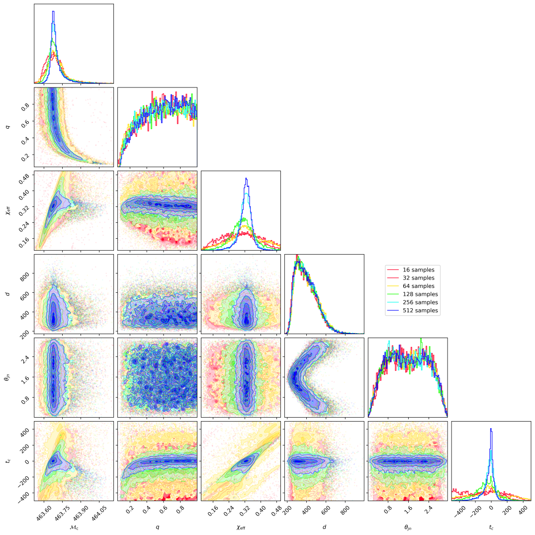
Figure 4: Downsampled posteriors of the fiducial system with $\Delta f/f_{\mathrm{max}}=0.9$, $N_{\mathrm{f}}=10^{6}$ (see Section 4.4.1 and Table 4.4.2). The posteriors converge as the number of samples is increased. Selected posteriors have been included to prevent a congested plot. There is almost no discernible difference between corner plots with $N_{\mathrm{s}}\geq 256$. As $N_{\mathrm{s}}$ decreases, we can clearly see the posterior ‘breaks down’, the few samples remaining being unable to constrain the parameters in the same way as the higher $N_{\mathrm{s}}$ posteriors.

References

- [1] John Baker et al. “The Laser Interferometer Space Antenna: Unveiling the Millihertz Gravitational Wave Sky”, 2019 arXiv:1907.06482 [astro-ph.IM]
- [2] Scott A. Hughes “Gravitational Waves from Merging Compact Binaries” In Annual Review of Astronomy and Astrophysics 47.1 Annual Reviews, 2009, pp. 107–157 DOI: 10.1146/annurev-astro-082708-101711
- [3] Stefan Grimm and Jan Harms “Multiband gravitational-wave parameter estimation: A study of future detectors” In Physical Review D 102.2 American Physical Society (APS), 2020 DOI: 10.1103/physrevd.102.022007
- [4] Chang Liu, Lijing Shao, Junjie Zhao and Yong Gao “Multiband observation of LIGO/Virgo binary black hole mergers in the gravitational-wave transient catalog GWTC-1” In Monthly Notices of the Royal Astronomical Society 496.1 Oxford University Press (OUP), 2020, pp. 182–196 DOI: 10.1093/mnras/staa1512
- [5] Scott E. Perkins, Nicolás Yunes and Emanuele Berti “Probing fundamental physics with gravitational waves: The next generation” In Physical Review D 103.4 American Physical Society (APS), 2021 DOI: 10.1103/physrevd.103.044024
- [6] Kaze W.. Wong, Ely D. Kovetz, Curt Cutler and Emanuele Berti “Expanding the LISA Horizon from the Ground” In Physical Review Letters 121.25 American Physical Society (APS), 2018 DOI: 10.1103/physrevlett.121.251102
- [7] Leor Barack and Curt Cutler “Using LISA extreme-mass-ratio inspiral sources to test off-Kerr deviations in the geometry of massive black holes” In Physical Review D 75.4 American Physical Society (APS), 2007 DOI: 10.1103/physrevd.75.042003
- [8] Lorenzo Speri and Jonathan R. Gair “Assessing the impact of transient orbital resonances” In Physical Review D 103.12 American Physical Society (APS), 2021 DOI: 10.1103/physrevd.103.124032
- [9] Michele Vallisneri “Use and abuse of the Fisher information matrix in the assessment of gravitational-wave parameter-estimation prospects” In Physical Review D 77.4 American Physical Society (APS), 2008 DOI: 10.1103/physrevd.77.042001
- [10] Carl L. Rodriguez, Benjamin Farr, Will M. Farr and Ilya Mandel “Inadequacies of the Fisher information matrix in gravitational-wave parameter estimation” In Physical Review D 88.8 American Physical Society (APS), 2013 DOI: 10.1103/physrevd.88.084013
- [11] Rory Smith et al. “Fast and accurate inference on gravitational waves from precessing compact binaries” In Physical Review D 94.4 American Physical Society (APS), 2016 DOI: 10.1103/physrevd.94.044031
- [12] Barak Zackay, Liang Dai and Tejaswi Venumadhav “Relative Binning and Fast Likelihood Evaluation for Gravitational Wave Parameter Estimation”, 2018 arXiv:1806.08792 [astro-ph.IM]
- [13] Soichiro Morisaki “Accelerating parameter estimation of gravitational waves from compact binary coalescence using adaptive frequency resolutions” In Physical Review D 104.4 American Physical Society (APS), 2021 DOI: 10.1103/physrevd.104.044062
- [14] Serena Vinciguerra, John Veitch and Ilya Mandel “Accelerating gravitational wave parameter estimation with multi-band template interpolation” In Classical and Quantum Gravity 34.11 IOP Publishing, 2017, pp. 115006 DOI: 10.1088/1361-6382/aa6d44
- [15] Neil J. Cornish “Time-frequency analysis of gravitational wave data” In Physical Review D 102.12 American Physical Society (APS), 2020 DOI: 10.1103/physrevd.102.124038
- [16] G Larry Bretthorst “Bayesian spectrum Analysis and parameter estimation” Springer-Verlag Berlin Heidelberg, 1988 URL: http://bayes.wustl.edu/glb/book.pdf
- [17] André Klein and Guy Mélard “Computation of the Fisher information matrix for time series models” In Journal of Computational and Applied Mathematics 64, 1995, pp. 57–68
- [18] Alan Heavens “Generalisations of Fisher Matrices” In Entropy 18.6 MDPI AG, 2016, pp. 236 DOI: 10.3390/e18060236
- [19] Daniel Foreman-Mackey, David W. Hogg, Dustin Lang and Jonathan Goodman “emcee: The MCMC Hammer” In Publications of the Astronomical Society of the Pacific 125.925 IOP Publishing, 2013, pp. 306–312 DOI: 10.1086/670067
- [20] Walter Del Pozzo and John Veitch “CPNest: Parallel nested sampling”, Astrophysics Source Code Library, record ascl:2205.021, 2022, pp. ascl:2205.021 ASCL: 2205.021
- [21] Joshua S. Speagle “DYNESTY: a dynamic nested sampling package for estimating Bayesian posteriors and evidences” In mnras 493.3, 2020, pp. 3132–3158 DOI: 10.1093/mnras/staa278
- [22] Michael J. Williams, John Veitch and Chris Messenger “Nested sampling with normalizing flows for gravitational-wave inference” In Physical Review D 103.10 American Physical Society (APS), 2021 DOI: 10.1103/physrevd.103.103006
- [23] Michael L. Katz et al. “GPU-accelerated massive black hole binary parameter estimation with LISA” In Physical Review D 102.2 American Physical Society (APS), 2020 DOI: 10.1103/physrevd.102.023033
- [24] Michele Vallisneri “Beyond Fisher: exact sampling distributions of the maximum-likelihood estimator in gravitational-wave parameter estimation”, 2011 arXiv:1108.1158 [gr-qc]
- [25] Héctor Estellés et al. “Phenomenological time domain model for dominant quadrupole gravitational wave signal of coalescing binary black holes” In Physical Review D 103.12 American Physical Society (APS), 2021 DOI: 10.1103/physrevd.103.124060
- [26] M. Maggiore “Gravitational Waves: Volume 1: Theory and Experiments”, Gravitational Waves OUP Oxford, 2008 URL: https://books.google.co.uk/books?id=AqVpQgAACAAJ
- [27] Gregory Ashton et al. “Bilby: A User-friendly Bayesian Inference Library for Gravitational-wave Astronomy” In The Astrophysical Journal Supplement Series 241.2 American Astronomical Society, 2019, pp. 27 DOI: 10.3847/1538-4365/ab06fc
- [28] Stefan Walt, S. Colbert and Gael Varoquaux “The NumPy Array: A Structure for Efficient Numerical Computation” In Computing in Science & Engineering 13.2, 2011, pp. 22–30 DOI: 10.1109/MCSE.2011.37
- [29] Pauli Virtanen, Ralf Gommers, Travis E. Oliphant and Matt Haberland “SciPy 1.0: fundamental algorithms for scientific computing in Python” In Nature Methods 17.3 Springer ScienceBusiness Media LLC, 2020, pp. 261–272 DOI: 10.1038/s41592-019-0686-2