Generalized framework for admissibility preserving Lax-Wendroff Flux Reconstruction for hyperbolic conservation laws with source terms

Arpit Babbar0000-0002-9453-370X and Praveen Chandrashekar0000-0003-1903-4107

1 Introduction

Lax-Wendroff (LW) methods are a class of single stage explicit high order methods for solving time dependent PDEs, and are an alternative to the PDE solvers where multistage explicit Runge-Kutta (RK) methods are used for temporal discretization. The single step nature of LW methods decreases inter-element communication and makes them suitable for modern memory bandwidth limited hardware. Arbitrary high order of accuracy is achieved in Lax-Wendroff schemes by performing a high order Taylor’s expansion of the solution and using the PDE to replace the temporal derivatives with a spatial derivative of the time-averaged flux approximation; the procedure is a generalization of Lax1960 . Some of the pioneering works are Qiu2003 ; Qiu2005b . Another class of single stage methods is ADER, where a high order element local solution is obtained by solving a space-time implicit equation Titarev2002 ; Dumbser2008 .

Flux Reconstruction (FR) is a collocation based, Spectral Element Method introduced by Huynh Huynh2007 and uses the same polynomial basis approximation as the Discontinuous Galerkin (DG) method of Cockburn and Shu cockburn2000 . The FR scheme is quadrature free and can generalize various numerical schemes including variants of DG by making different choices of correction functions and solution points Huynh2007 ; Trojak2021 . The accuracy and stability of FR has been studied in Huynh2007 ; Vincent2011a ; Trojak2021 ; Cicchino2022a .

LW schemes with FR spatial approximation were first introduced in Lou2020 , the role of FR in these schemes is to correct the time averaged flux while coupling elements across interfaces. In babbar2022 , the present authors proposed a Lax-Wendroff Flux Reconstruction (LWFR) scheme using the Jacobian-free approximate Lax-Wendroff procedure of Zorio2017 ; Burger2017 . The numerical flux was carefully constructed in babbar2022 to obtain enhanced accuracy and stability. In babbar2023admissibility , a subcell based shock capturing blending scheme was introduced for LWFR based on hennemann2021 . babbar2023admissibility exploited the subcell structure to construct a blended numerical flux between the time averaged flux and the low order flux, which was used to obtain provably admissibility preserving property of the Lax-Wendroff scheme.

In this work, it is shown that the construction of blended numerical flux to enforce admissibility can also be done when there is no subcell based limiting scheme. The initial argument is similar to performing a decomposition of the cell average into fictitious finite volume updates as in Zhang2010b ; zhang2010c . The difference from Zhang2010b arises in the case of LW schemes as some of the fictitious finite volume updates involve the LW high order fluxes. Then, it is seen that, if the LW numerical flux is limited to ensure that the update with its fictitious finite volume fluxes is admissible, the scheme will be admissibility preserving in means. The limiting procedure of babbar2023admissibility is then used to enforce admissibility.

To numerically validate our claim, we test LWFR on the Ten Moment equations, which are derived by Levermore et al. Levermore_1996 by taking a Gaussian closure of the kinetic model. These equations are relevant in many applications, especially related to plasma flows (see Berthon_TMP_2006 ; Berthon2015 and further references in meena2017 ), in cases where the local thermodynamic equilibrium used to close the Euler equations of compressible flows is not valid, and anisotropic nature of the pressure needs to be accounted for. The Ten Moment equations model is a hyperbolic conservation law with source terms. Thus, in addition to showing that our positivity preserving framework preserves admissibility in the presence of shocks and rarefactions, we also introduce the first LWFR scheme in the presence of source terms. The approach involves adding time averages of the sources and thus we also propose a source term limiting procedure so that admissibility is still maintained.

The rest of the paper is organized as follows. Section 2 is a review of LWFR scheme and notions of admissibility preservation. Section 3 describes the additional limiting required in LW scheme for admissibility preservation, i.e., for the time averaged flux (Section 3.1) and time averaged sources (Section 3.2). Section 4 shows the numerical results for the Ten Moment equations model and conclusions of the work are drawn in Section 5.

2 Lax-Wendroff Flux Reconstruction

Consider a conservation law of the form

$$\boldsymbol{u}_{t}+\boldsymbol{f}_{x}=\boldsymbol{s}$$ (1)

where $\boldsymbol{u}\in\mathbb{R}^{p}$ is the vector of conserved quantities, $\boldsymbol{f}=\boldsymbol{f}(\boldsymbol{u})$ is the corresponding flux, $\boldsymbol{s}=\boldsymbol{s}\left(\boldsymbol{u},t,x\right)$ is the source term, together with some initial and boundary conditions. The solution that is physically correct is assumed to belong to an admissibility set, denoted by $\mathcal{U}_{\textrm{$\operatorname{ad}$}}$. For example in case of compressible flows, the density and pressure (or internal energy) must remain positive. In case of the Ten Moment equations (18), the density must remain positive and the pressure tensor $\boldsymbol{p}$ must be positive definite. In both these models, and most of the models that are of interest, the admissibility set is a convex subset of $\mathbb{R}^{p}$, and can be written as

$$\mathcal{U}_{\textrm{$\operatorname{ad}$}}=\{\boldsymbol{u}\in\mathbb{R}^{p}:P_{k}(\boldsymbol{u})>0,1\leq k\leq K\}$$ (2)

For Euler’s equations, $K=2$ and $P_{1},P_{2}$ are density, pressure functions respectively; if the density is positive then pressure is a concave function of the conserved variables. For the Ten Moment equations (18), $K=3$ and $P_{1},P_{2},P_{3}$ are density, $\operatorname{trace}\left(\boldsymbol{p}\right)$, $\det\left(\boldsymbol{p}\right)$. Although density and trace functions are concave functions of the conserved variables, $\det\left(\boldsymbol{p}\right)$ is not so.

For the numerical solution, we will divide the computational domain $\Omega$ into disjoint elements $\Omega_{e}$, with $\Omega_{e}=[x_{e-\frac{1}{2}},x_{e+\frac{1}{2}}]$ so that $\Delta x_{e}=x_{e+\frac{1}{2}}-x_{e-\frac{1}{2}}$. Then, we map each element $\Omega_{e}$ to the reference element $[0,1]$ by $x\mapsto\frac{x-x_{e-1/2}}{\Delta x_{e}}=:\xi$. Inside each element, we approximate the solution by degree $N\geq 0$ polynomials belonging to the set $\mathbb{P}_{N}$. For this, choose $N+1$ distinct nodes $\{\xi_{i}\}_{i=0}^{N}$ in $[0,1]$ which will be taken to be Gauss-Legendre (GL) points in this work, and will also be referred to as solution points. The solution inside an element $\Omega_{e}$ is given by $\boldsymbol{u}_{h}(\xi,t)=\sum_{p=0}^{N}\boldsymbol{u}_{e,p}(t)\ell_{p}(\xi)$ where $\{\ell_{p}\}$ are Lagrange polynomials of degree $N$ defined to satisfy $\ell_{p}(\xi_{q})=\delta_{pq}$. Note that the coefficients $\boldsymbol{u}_{e,p}$ which are the basic unknowns or degrees of freedom (dof), are the solution values at the solution points.

The Lax-Wendroff scheme combines the spatial and temporal discretization into a single step. The starting point is a Taylor’s expansion in time following the Cauchy-Kowalewski procedure where the PDE is used to rewrite some of the temporal derivatives in the Taylor expansion as spatial derivatives. Using Taylor’s expansion in time around $t=t_{n}$, we can write the solution at the next time level as

$$\boldsymbol{u}^{n+1}=\boldsymbol{u}^{n}+\sum_{m=1}^{N+1}\frac{\Delta t^{m}}{m!}\partial_{t}^{m}\boldsymbol{u}^{n}+O(\Delta t^{N+2})$$

Since the spatial error is expected to be of $O(\Delta x^{N+1})$, we retain terms up to $O(\Delta t^{N+1})$ in the Taylor expansion, so that the overall formal accuracy is of order $N+1$ in both space and time. Using the PDE, $\partial_{t}\boldsymbol{u}=-\partial_{x}\boldsymbol{f}+\boldsymbol{s}$, we re-write time derivatives of the solution in terms of spatial derivatives of the flux and source terms

$$\partial_{t}^{m}\boldsymbol{u}=-(\partial_{t}^{m-1}\boldsymbol{f})_{x}+\partial_{t}^{m-1}\boldsymbol{s},\qquad m=1,2,\ldots$$

so that

$$\begin{split}\boldsymbol{u}^{n+1}&=\boldsymbol{u}^{n}-\sum_{m=1}^{N+1}\frac{\Delta t^{m}}{m!}(\partial_{t}^{m-1}\boldsymbol{f})_{x}+\sum_{m=1}^{N+1}\frac{\Delta t^{m}}{m!}\partial_{t}^{m-1}\boldsymbol{s}+O(\Delta t^{N+2})\\ &=\boldsymbol{u}^{n}-\Delta t\frac{\partial\boldsymbol{F}}{\partial x}(\boldsymbol{u}^{n})+\Delta t\boldsymbol{S}\left(\boldsymbol{u}^{n},t^{n}\right)+O(\Delta t^{N+2})\end{split}$$ (3)

where

$$\boldsymbol{F} =\sum_{m=0}^{N}\frac{\Delta t^{m}}{(m+1)!}\partial_{t}^{m}\boldsymbol{f}=\boldsymbol{f}+\frac{\Delta t}{2}\partial_{t}\boldsymbol{f}+\ldots+\frac{\Delta t^{N}}{(N+1)!}\partial_{t}^{N}\boldsymbol{f}$$ (4)

$$\boldsymbol{S} =\sum_{m=0}^{N}\frac{\Delta t^{m}}{(m+1)!}\partial_{t}^{m}\boldsymbol{s}=\boldsymbol{s}+\frac{\Delta t}{2}\partial_{t}\boldsymbol{s}+\ldots+\frac{\Delta t^{N}}{(N+1)!}\partial_{t}^{N}\boldsymbol{s}$$ (5)

Note that $\boldsymbol{F}({\boldsymbol{u}^{n}}),\boldsymbol{S}(\boldsymbol{u}^{n},t^{n})$ are approximations to the time average flux and source term in the interval $[t_{n},t_{n+1}]$ since they can be written as

$$\boldsymbol{F}({\boldsymbol{u}^{n}}) =\frac{1}{\Delta t}\int_{t_{n}}^{t_{n+1}}\left[\boldsymbol{f}(\boldsymbol{u}^{n})+\ldots+\frac{(t-t_{n})^{N}}{N!}\partial_{t}^{N}\boldsymbol{f}(\boldsymbol{u}^{n})\right]dt$$ (6)

$$\boldsymbol{S}({\boldsymbol{u}^{n}},t^{n}) =\frac{1}{\Delta t}\int_{t_{n}}^{t_{n+1}}\left[\boldsymbol{s}(\boldsymbol{u}^{n},t^{n})+\ldots+\frac{(t-t_{n})^{N}}{N!}\partial_{t}^{N}\boldsymbol{s}(\boldsymbol{u}^{n},t^{n})\right]dt$$ (7)

where the quantity inside the square brackets is the truncated Taylor expansion of the flux $\boldsymbol{f}$ or source $\boldsymbol{s}$ in time. Following equation (3) we need to specify the construction of the time averaged flux (4) and the time averaged source terms (5). The first step of approximating (3) is the predictor step where a locally degree $N$ approximation $\boldsymbol{F}^{\delta}$ of the time averaged flux is computed by the approximate Lax-Wendroff procedure of Zorio Zorio2017 , also discussed in Section 4.4 of babbar2022 . Then, as in the standard RKFR scheme, we perform the Flux Reconstruction procedure on $\boldsymbol{F}^{\delta}$ to construct a locally degree $N+1$ and globally continuous flux approximation $\boldsymbol{F}_{h}(\xi)$. The time average source $\boldsymbol{S}$ will also be approximated locally as a degree $N$ polynomial using the approximate Lax-Wendroff procedure and denoted with a single notation $\boldsymbol{S}^{\delta}(\xi)$ since it needs no correction. The scheme for local approximation is discussed in Section 2.1. After computing $\boldsymbol{F}_{h},\boldsymbol{S}^{\delta}$, truncating equation (3), the solution at the nodes is updated by a collocation scheme as follows

$$\boldsymbol{u}_{e,p}^{n+1}=\boldsymbol{u}_{e,p}^{n}-\frac{\Delta t}{\Delta x_{e}}\frac{d\boldsymbol{F}_{h}}{d\xi}(\xi_{p})+\Delta t\boldsymbol{S}^{\delta}(\xi_{p}),\qquad 0\leq p\leq N$$ (8)

This is the single step Lax-Wendroff update scheme for any order of accuracy.

2.1 Approximate Lax-Wendroff procedure for degree $N=2$

The approximations of temporal derivatives of $\boldsymbol{s}$ are made in a similar fashion as those of $\boldsymbol{f}$ in Zorio2017 ; babbar2022 . For example, to obtain second order accuracy, $\partial_{t}\boldsymbol{s}$ can be approximated as

$$\partial_{t}\boldsymbol{s}\left(\boldsymbol{u},\boldsymbol{x},t\right) \approx\frac{\boldsymbol{s}\left(\boldsymbol{u}^{n}+\Delta t\boldsymbol{u}^{n}_{t},\boldsymbol{x},t^{n+1}\right)-\boldsymbol{s}\left(\boldsymbol{u}^{n}-\Delta t\boldsymbol{u}_{t}^{n},\boldsymbol{x},t^{n-1}\right)}{2\Delta t}$$

where $\boldsymbol{u}_{t}=-\partial_{x}\boldsymbol{f}+\boldsymbol{s}\left(\boldsymbol{u},\boldsymbol{x},t\right)$. Denoting ${\text{{\hskip 1.00006pt}g{\hskip 1.49994pt}}}^{(k)}$ as an approximation for $\Delta t^{k}\partial_{t}g$, we explain the local flux and source term approximation procedure for degree $N=2$

$$\text{{\hskip 1.00006pt}F{\hskip 1.49994pt}}=\text{{\hskip 1.00006pt}f{\hskip 1.49994pt}}+\frac{1}{2}\text{{\hskip 1.00006pt}f{\hskip 1.49994pt}}^{(1)}+\frac{1}{6}\text{{\hskip 1.00006pt}f{\hskip 1.49994pt}}^{(2)},\qquad\text{{\hskip 1.00006pt}S{\hskip 1.49994pt}}=\text{{\hskip 1.00006pt}s{\hskip 1.49994pt}}+\frac{1}{2}\text{{\hskip 1.00006pt}s{\hskip 1.49994pt}}^{(1)}+\frac{1}{6}\text{{\hskip 1.00006pt}s{\hskip 1.49994pt}}^{(2)}$$

where

$$\text{{\hskip 1.00006pt}u{\hskip 1.49994pt}}^{(1)} = -\frac{\Delta t}{\Delta x_{e}}\text{{\hskip 1.00006pt}D{\hskip 1.49994pt}}\text{{\hskip 1.00006pt}f{\hskip 1.49994pt}}+\Delta t\text{{\hskip 1.00006pt}s{\hskip 1.49994pt}}$$

$$\text{{\hskip 1.00006pt}f{\hskip 1.49994pt}}^{(1)},\text{{\hskip 1.00006pt}s{\hskip 1.49994pt}}^{(1)} = \frac{1}{2}\left[\boldsymbol{f}\left(\text{{\hskip 1.00006pt}u{\hskip 1.49994pt}}+\text{{\hskip 1.00006pt}u{\hskip 1.49994pt}}^{(1)}\right)-\boldsymbol{f}\left(\text{{\hskip 1.00006pt}u{\hskip 1.49994pt}}-\text{{\hskip 1.00006pt}u{\hskip 1.49994pt}}^{(1)}\right)\right],\frac{1}{2}\left[\boldsymbol{s}\left(\text{{\hskip 1.00006pt}u{\hskip 1.49994pt}}+\text{{\hskip 1.00006pt}u{\hskip 1.49994pt}}^{(1)}\right)-\boldsymbol{s}\left(\text{{\hskip 1.00006pt}u{\hskip 1.49994pt}}-\text{{\hskip 1.00006pt}u{\hskip 1.49994pt}}^{(1)}\right)\right]$$

$$\text{{\hskip 1.00006pt}u{\hskip 1.49994pt}}^{(2)} = -\frac{\Delta t}{\Delta x_{e}}\text{{\hskip 1.00006pt}D{\hskip 1.49994pt}}\text{{\hskip 1.00006pt}f{\hskip 1.49994pt}}^{(1)}+\Delta t\text{{\hskip 1.00006pt}s{\hskip 1.49994pt}}^{(1)}$$

$$\text{{\hskip 1.00006pt}f{\hskip 1.49994pt}}^{(2)} = \boldsymbol{f}\left(\text{{\hskip 1.00006pt}u{\hskip 1.49994pt}}+\text{{\hskip 1.00006pt}u{\hskip 1.49994pt}}^{(1)}+\frac{1}{2}\text{{\hskip 1.00006pt}u{\hskip 1.49994pt}}^{(2)}\right)-2\boldsymbol{f}(\text{{\hskip 1.00006pt}u{\hskip 1.49994pt}})+\boldsymbol{f}\left(\text{{\hskip 1.00006pt}u{\hskip 1.49994pt}}-\text{{\hskip 1.00006pt}u{\hskip 1.49994pt}}^{(1)}+\frac{1}{2}\text{{\hskip 1.00006pt}u{\hskip 1.49994pt}}^{(2)}\right)$$

$$\text{{\hskip 1.00006pt}s{\hskip 1.49994pt}}^{(2)} = \boldsymbol{s}\left(\text{{\hskip 1.00006pt}u{\hskip 1.49994pt}}+\text{{\hskip 1.00006pt}u{\hskip 1.49994pt}}^{(1)}+\frac{1}{2}\text{{\hskip 1.00006pt}u{\hskip 1.49994pt}}^{(2)}\right)-2\boldsymbol{s}(\text{{\hskip 1.00006pt}u{\hskip 1.49994pt}})+\boldsymbol{s}\left(\text{{\hskip 1.00006pt}u{\hskip 1.49994pt}}-\text{{\hskip 1.00006pt}u{\hskip 1.49994pt}}^{(1)}+\frac{1}{2}\text{{\hskip 1.00006pt}u{\hskip 1.49994pt}}^{(2)}\right)$$

For complete details on the local approximation of the flux $\boldsymbol{F}$ for all degrees and then its FR correction using the time numerical flux $\boldsymbol{F}_{e+\frac{1}{2}}$, the reader is referred to babbar2022 .

2.2 Admissibility preservation

The admissibility preserving property of the conservation law, also known as convex set preservation property since $\mathcal{U}_{\textrm{$\operatorname{ad}$}}$ is convex, can be written as

$$\boldsymbol{u}(\cdot,t_{0})\in\mathcal{U}_{\textrm{$\operatorname{ad}$}}\qquad\Longrightarrow\qquad\boldsymbol{u}(\cdot,t)\in\mathcal{U}_{\textrm{$\operatorname{ad}$}},\qquad t>t_{0}$$ (9)

Thus, an admissibility preserving FR scheme is one which preserves admissibility at all solution points (Definition 1 of babbar2023admissibility ). In this work, as in babbar2023admissibility , we study the admissibility preservation in means property of the LWFR scheme (Definition 2 of babbar2023admissibility ) which is said to hold for schemes that satisfy

$$\boldsymbol{u}_{e,p}^{n}\in\mathcal{U}_{\textrm{$\operatorname{ad}$}}\quad\forall e,p\qquad\Longrightarrow\qquad\overline{\boldsymbol{u}}_{e}^{n+1}\in\mathcal{U}_{\textrm{$\operatorname{ad}$}}\quad\forall e$$ (10)

where $\overline{\boldsymbol{u}}_{e}:=\sum_{p=0}^{N}w_{p}\boldsymbol{u}_{e,p}$ denotes the cell average of $\boldsymbol{u}_{e}$. Once the scheme is admissibility preserving in means, the scaling limiter of Zhang2010b can be used to obtain an admissibility preserving scheme. The following property of the LWFR scheme will be crucial in the obtaining admissibility preservation in means

$$\overline{\boldsymbol{u}}_{e}^{n+1}=\overline{\boldsymbol{u}}_{e}^{n}-\frac{\Delta t}{\Delta x_{e}}(\boldsymbol{F}_{e+\frac{1}{2}}-\boldsymbol{F}_{e-\frac{1}{2}})+\Delta t\overline{\boldsymbol{S}}_{e}$$ (11)

where $\overline{\boldsymbol{S}}_{e}:=\sum_{p=0}^{N}w_{p}\boldsymbol{S}_{e}^{\delta}(\xi_{p})$ is the cell average of the source term.

3 Limiting time averages

3.1 Limiting time average flux

In this section, we study admissibility preservation in means property (10) for the LWFR update (8) in the case where source term $\boldsymbol{s}$ in (1) is zero. Similar to the work of Zhang-Shu Zhang2010b , we define fictitious finite volume updates

$$\begin{split}\invbreve{\boldsymbol{u}}_{e,0}^{n+1}&=\boldsymbol{u}_{e,0}^{n}-\frac{\Delta t}{w_{0}\Delta x_{e}}[\boldsymbol{f}_{\frac{1}{2}}^{e}-\boldsymbol{F}_{e-\frac{1}{2}}^{\operatorname{LW}}]\\ \invbreve{\boldsymbol{u}}_{e,p}^{n+1}&=\boldsymbol{u}_{e,p}^{n}-\frac{\Delta t}{w_{p}\Delta x_{e}}[\boldsymbol{f}_{p+\frac{1}{2}}^{e}-\boldsymbol{f}_{p-\frac{1}{2}}^{e}],\qquad 1\leq p\leq N-1\\ \invbreve{\boldsymbol{u}}_{e,N}^{n+1}&=\boldsymbol{u}_{e,N}^{n}-\frac{\Delta t}{w_{N}\Delta x_{e}}[\boldsymbol{F}_{e+\frac{1}{2}}^{\operatorname{LW}}-\boldsymbol{f}_{N-\frac{1}{2}}^{e}]\end{split}$$ (12)

where $\boldsymbol{f}_{p+\frac{1}{2}}^{e}=\boldsymbol{f}(\boldsymbol{u}_{e,p}^{n},\boldsymbol{u}_{e,p+1}^{n})$ is an admissibility preserving finite volume numerical flux. Then, note that

$$\overline{\boldsymbol{u}}_{e}^{n+1}=\sum_{p=0}^{N}w_{p}\invbreve{\boldsymbol{u}}_{e,p}^{n+1}$$ (13)

Thus, if we can ensure that $\invbreve{\boldsymbol{u}}_{e,p}^{n+1}\in\mathcal{U}_{\textrm{$\operatorname{ad}$}}$ for all $p$, the scheme will be admissibility preserving in means (10). We do have $\invbreve{\boldsymbol{u}}_{e,p}^{n+1}\in\mathcal{U}_{\textrm{$\operatorname{ad}$}}$ for $1\leq p\leq N-1$ under appropriate CFL conditions because the finite volume fluxes are admissibility preserving. In order to ensure that the updates $\invbreve{\boldsymbol{u}}_{e,0}^{n+1},\invbreve{\boldsymbol{u}}_{e,N}^{n+1}$ are also admissible, the flux limiting procedure of babbar2023admissibility is followed so that the high order numerical fluxes $\boldsymbol{F}_{e\pm\frac{1}{2}}^{\operatorname{LW}}$ are replaced by blended numerical fluxes $\boldsymbol{F}_{e\pm\frac{1}{2}}$. The procedure is explained here for completeness. We define an admissibility preserving lower order flux at the interface $e+\frac{1}{2}$

$$\boldsymbol{f}_{e+\frac{1}{2}}=\boldsymbol{f}(\boldsymbol{u}_{e+1,0}^{n},\boldsymbol{u}_{e,N}^{n})$$

Note that, for an RKFR scheme using Gauss-Legendre-Lobatto (GLL) solution points, the definition of $\invbreve{\boldsymbol{u}}_{e,N}^{n+1}$ will use $\boldsymbol{f}_{e+\frac{1}{2}}$ in place of $\boldsymbol{F}_{e+\frac{1}{2}}^{\operatorname{LW}}$ and thus admissibility preserving in means property will always be present. That is the argument of Zhang2010b and here we demonstrate that the same argument can be applied to LWFR schemes by limiting $\boldsymbol{F}_{e+\frac{1}{2}}^{\text{LW}}$. We will explain the procedure for limiting $\boldsymbol{F}_{e+\frac{1}{2}}^{\operatorname{LW}}$ to obtain $\boldsymbol{F}_{e+\frac{1}{2}}$; it will be similar in the case of $\boldsymbol{F}_{e-\frac{1}{2}}$. Note that we want $\boldsymbol{F}_{e+\frac{1}{2}}$ to be such that the following are admissible

$$\begin{split}\invbreve{\boldsymbol{u}}_{0}^{n+1}&=\boldsymbol{u}_{e+1,0}^{n}-\frac{\Delta t}{w_{0}\Delta x_{e+1}}(\boldsymbol{f}^{e+1}_{\frac{1}{2}}-\boldsymbol{F}_{e+\frac{1}{2}})\\ \invbreve{\boldsymbol{u}}_{N}^{n+1}&=\boldsymbol{u}_{e,N}^{n}-\frac{\Delta t}{w_{N}\Delta x_{e}}(\boldsymbol{F}_{e+\frac{1}{2}}-\boldsymbol{f}^{e}_{N-\frac{1}{2}})\end{split}$$ (14)

We will exploit the admissibility preserving property of the finite volume fluxes to get

$$\invbreve{\boldsymbol{u}}^{\operatorname{low},n+1}_{0} =\boldsymbol{u}_{e+1,0}^{n}-\frac{\Delta t}{w_{0}\Delta x_{e+1}}(\boldsymbol{f}^{e+1}_{\frac{1}{2}}-\boldsymbol{f}_{e+\frac{1}{2}})\in\mathcal{U}_{\textrm{$\operatorname{ad}$}}$$

$$\invbreve{\boldsymbol{u}}^{\operatorname{low},n+1}_{N} =\boldsymbol{u}_{e,N}^{n}-\frac{\Delta t}{w_{N}\Delta x_{e}}(\boldsymbol{f}_{e+\frac{1}{2}}-\boldsymbol{f}^{e}_{N-\frac{1}{2}})\in\mathcal{U}_{\textrm{$\operatorname{ad}$}}$$

Let $\{P_{k},1\leq 1\leq K\}$ be the admissibility constraints (2) of (1). The time averaged flux is limited by iterating over the constraints. For each constraint, we can solve an optimization problem to find the largest $\theta\in[0,1]$ satisfying

$$P_{k}(\theta\invbreve{\boldsymbol{u}}_{p}^{n+1}+(1-\theta)\invbreve{\boldsymbol{u}}^{\operatorname{low},n+1}_{p})>\epsilon_{p},\qquad p=0,N$$ (15)

where $\epsilon_{p}$ is a tolerance, taken to be $\frac{1}{10}P_{k}(\invbreve{\boldsymbol{u}}^{\operatorname{low},n+1}_{p})$ ramirez2021 . The optimization problem is usually a polynomial equation in $\theta$. If $P_{k}$ is a concave function of the conserved variables, we can follow babbar2023admissibility and use the simpler but possibly sub-optimal approach of defining

$$\theta=\min\left(\min_{p=0,N}\left|\frac{\epsilon_{p}-P_{k}(\invbreve{\boldsymbol{u}}_{p}^{\text{low},n+1})}{P_{k}(\invbreve{\boldsymbol{u}}_{p}^{n+1})-P_{k}(\invbreve{\boldsymbol{u}}_{p}^{\text{low},n+1})}\right|,1\right)$$ (16)

In either case, by iterating over the admissibility constraints $\{P_{k}\}$ of the conservation law, the flux $\boldsymbol{F}_{e+\frac{1}{2}}^{\operatorname{LW}}$ can be corrected as in Algorithm 1.

Algorithm 1 Flux limiting

$\boldsymbol{F}_{e+\frac{1}{2}}\leftarrow\boldsymbol{F}_{e+\frac{1}{2}}^{\operatorname{LW}}$

for $k$=1:$K$ do

     $\epsilon_{0},\epsilon_{N}\leftarrow\frac{1}{10}P_{k}(\invbreve{\boldsymbol{u}}^{\operatorname{low},n+1}_{0}),\frac{1}{10}P_{k}(\invbreve{\boldsymbol{u}}^{\operatorname{low},n+1}_{N})$

     $\operatorname{Find}\theta$ by solving the optimization problem (15) or by using (16) if $P_{k}$ is concave

     $\boldsymbol{F}_{e+\frac{1}{2}}\leftarrow\theta\boldsymbol{F}_{e+\frac{1}{2}}+(1-\theta)\boldsymbol{f}_{e+\frac{1}{2}}$

     $\invbreve{\boldsymbol{u}}_{0}^{n+1}\leftarrow\boldsymbol{u}_{e+1,0}^{n}-\frac{\Delta t}{w_{0}\Delta x_{e+1}}(\boldsymbol{f}^{e+1}_{\frac{1}{2}}-\boldsymbol{F}_{e+\frac{1}{2}})$

     $\invbreve{\boldsymbol{u}}_{N}^{n+1}\leftarrow\boldsymbol{u}_{e,N}^{n}-\frac{\Delta t}{w_{N}\Delta x_{e}}(\boldsymbol{F}_{e+\frac{1}{2}}-\boldsymbol{f}^{e}_{N-\frac{1}{2}})$

end for

After $K$ iterations, we will have $P_{k}(\invbreve{\boldsymbol{u}}_{p}^{n+1})\geq\epsilon_{p}$ for $p=0,N$ and $1\leq k\leq K$. Once this procedure is done at all the interfaces, i.e., after Algorithm 1 is performed, using the numerical flux $\boldsymbol{F}_{e+\frac{1}{2}}$ in the LWFR scheme will ensure that $\invbreve{\boldsymbol{u}}_{e,p}^{n+1}$ (12) belongs to $\mathcal{U}_{\textrm{$\operatorname{ad}$}}$ for all $p$, implying $\overline{\boldsymbol{u}}_{e}^{n+1}\in\mathcal{U}_{\textrm{$\operatorname{ad}$}}$ by (13). Then, we can use the scaling limiter of Zhang2010b at all solution points and obtain an admissibility preserving LWFR scheme for conservation laws in the absence of source terms.

3.2 Limiting time average sources

After the flux limiting performed in Section 3.1, we will have an admissibility preserving in means scheme (10) if the source term average $\overline{\boldsymbol{S}}_{e}$ in (11) is zero. In order to get an admissibility preserving scheme in the presence of source terms, we will make a splitting of the cell average update (11), which is similar to that of meena2017

$$\overline{\boldsymbol{u}}^{n+1}_{e}=\frac{1}{2}\left(\overline{\boldsymbol{u}}^{n}_{e}-\frac{2\Delta t}{\Delta x_{e}}(\boldsymbol{F}_{e+\frac{1}{2}}-\boldsymbol{F}_{e-\frac{1}{2}})\right)+\frac{1}{2}(\overline{\boldsymbol{u}}^{n}_{e}+2\Delta t\overline{\boldsymbol{S}^{\text{LW}}_{e}})=:\overline{\boldsymbol{u}}^{\boldsymbol{F}}_{e}+\overline{\boldsymbol{u}}^{\boldsymbol{S}^{\text{LW}}}_{e}$$ (17)

where $\boldsymbol{S}^{\operatorname{LW}}_{e}$ denotes the time average source term in element $e$ computed with the approximate Lax-Wendroff procedure in Section 2.1. With the flux limiting performed in Section 3.1, we can ensure that cell average $\overline{\boldsymbol{u}}^{\boldsymbol{F}}_{e}\in\mathcal{U}_{\textrm{$\operatorname{ad}$}}$ if twice the standard CFL is assumed (although, in the experiments we conducted, the CFL restriction used in babbar2023admissibility preserved admissibility). In order to enforce $\overline{\boldsymbol{u}}^{\boldsymbol{S}}_{e}\in\mathcal{U}_{\textrm{$\operatorname{ad}$}}$, $\boldsymbol{S}^{\text{LW}}_{e}$ will be limited as follows. We will use the admissibility of the first order update using the source term

$$\overline{\boldsymbol{u}}^{\operatorname{low},n+1}_{e}:=\overline{\boldsymbol{u}}^{n}_{e}+2\Delta t\overline{\boldsymbol{s}}_{e}\in\mathcal{U}_{\textrm{$\operatorname{ad}$}},\qquad\overline{\boldsymbol{s}}_{e}=\sum_{p=0}^{N}w_{p}\boldsymbol{s}(\boldsymbol{u}_{e,p},\boldsymbol{x}_{e,p},t^{n})$$

which will be true under some problem dependent time step restrictions (e.g., Theorem 3.3.1 of Meena_Kumar_Chandrashekar_2017 ). Then, we will find a $\theta\in[0,1]$ so that for $\boldsymbol{S}=\theta\boldsymbol{s}+(1-\theta)\boldsymbol{S}^{\text{LW}}$, we will have $\overline{\boldsymbol{u}}_{e}^{\boldsymbol{S}}\in\mathcal{U}_{\textrm{$\operatorname{ad}$}}$. The $\theta$ can be found by iterating over admissibility constraints and using (15) or (16) where, for the first iteration, $\invbreve{\boldsymbol{u}}_{p}^{\text{low},n+1}$ is replaced by $\overline{\boldsymbol{u}}^{\operatorname{low},n+1}_{e}$ and $\invbreve{\boldsymbol{u}}_{p}^{n+1}$ by $\overline{\boldsymbol{u}}^{\boldsymbol{S}^{\text{LW}}}_{e}$. Thus, a procedure analogous to Algorithm 1 is used for limiting source terms. Then, replacing $\boldsymbol{S}^{\text{LW}}$ by $\boldsymbol{S}$ in (17), we will have $\overline{\boldsymbol{u}}^{\boldsymbol{S}}\in\mathcal{U}_{\textrm{$\operatorname{ad}$}}$ and since $\boldsymbol{F}$ has been corrected to ensure $\overline{\boldsymbol{u}}^{\boldsymbol{F}}_{e}\in\mathcal{U}_{\textrm{$\operatorname{ad}$}}$, we will also have $\overline{\boldsymbol{u}}^{n+1}_{e}\in\mathcal{U}_{\textrm{$\operatorname{ad}$}}$. Thus, we have an admissibility preserving in means LWFR scheme (10) even in the presence of source terms.

4 Numerical results

The numerical verification of admissibility preserving flux limiter (Section 3.1) and admissibility of LWFR with source terms (Section 3.2) is made through the Ten Moment equations Levermore_1996 which we describe here. Here, the energy tensor is defined by the ideal equation of state $\boldsymbol{E}=\frac{1}{2}\boldsymbol{p}+\frac{1}{2}\rho\boldsymbol{v}\otimes\boldsymbol{v}$ where $\rho$ is the density, $\boldsymbol{v}$ is the velocity vector, $\boldsymbol{p}$ is the symmetric pressure tensor. Thus, we can define the 2-D conservation law with source terms

$$\partial_{t}\boldsymbol{u}+\partial_{x_{1}}\boldsymbol{f}_{1}+\partial_{x_{2}}\boldsymbol{f}_{2}=\boldsymbol{s}^{x_{1}}\left(\boldsymbol{u}\right)+\boldsymbol{s}^{x_{2}}\left(\boldsymbol{u}\right)$$

where $\boldsymbol{u}=(\rho,\rho v_{1},\rho v_{2},E_{11},E_{12},E_{22})$ and

$$\boldsymbol{f}_{1}=\left[\begin{array}[]{c}\rho v_{1}\\ p_{11}+\rho v_{1}^{2}\\ p_{12}+\rho v_{1}v_{2}\\ \left(E_{11}+p_{11}\right)v_{1}\\ E_{12}v_{1}+\frac{1}{2}(p_{11}v_{2}+p_{12}v_{1})\\ E_{22}v_{1}+p_{12}v_{2}\end{array}\right],\quad\boldsymbol{f}_{2}=\left[\begin{array}[]{c}\rho v_{2}\\ p_{12}+\rho v_{1}v_{2}\\ p_{22}+\rho v_{2}^{2}\\ E_{11}v_{2}+p_{12}v_{1}\\ E_{12}v_{2}+\frac{1}{2}(p_{12}v_{2}+p_{22}v_{1})\\ \left(E_{22}+p_{22}\right)v_{2}\end{array}\right]$$ (18)

The source terms are given by

$$\boldsymbol{s}^{x_{1}}=\left[\begin{array}[]{c}0\\ -\frac{1}{2}\rho\partial_{x}W\\ 0\\ -\frac{1}{2}\rho v_{1}\partial_{x}W\\ -\frac{1}{4}\rho v_{2}\partial_{x}W\\ 0\end{array}\right],\qquad\boldsymbol{s}^{x_{2}}=\left[\begin{array}[]{c}0\\ 0\\ -\frac{1}{2}\rho\partial_{y}W\\ 0\\ -\frac{1}{4}\rho v_{1}\partial_{y}W\\ -\frac{1}{2}\rho v_{2}\partial_{y}W\end{array}\right]$$ (19)

where $W(x,y,t)$ is a given function, which models electron quiver energy in the laser Berthon2015 . The admissibility set is given by

$$\mathcal{U}_{\textrm{$\operatorname{ad}$}}=\left\{\boldsymbol{u}\in\mathbb{R}^{6}|\rho\left(\boldsymbol{u}\right)>0,\quad\boldsymbol{x}^{T}\boldsymbol{p}\left(\boldsymbol{u}\right)\boldsymbol{x}>0,\quad\boldsymbol{x}\in\mathbb{R}^{2}\backslash\left\{\boldsymbol{0}\right\}\right\}$$

which contains the states $\boldsymbol{u}$ with positive density and positive definite pressure tensor. The positive defininess of $\boldsymbol{p}$ implies that $p_{11}+p_{22}>0$ and $\det\boldsymbol{p}=p_{11}p_{22}-p_{12}^{2}>0$. The hyperbolicity of the system without source terms, along with its eigenvalues are presented in Lemma 2.0.2 of Meena_Kumar_Chandrashekar_2017 . The conditions for admissibiltiy preservation of the forward Euler method for the source terms, which are the basis for the source term limiting described in Section 3.2, are in Theorem 3.3.1 of Meena_Kumar_Chandrashekar_2017 . All distinct numerical experiments from Meena_Kumar_Chandrashekar_2017 ; meena2017 ; Meena2020 were performed and observed to validate the accuracy and robustness of the proposed scheme, but only some are shown here. The experiments were performed both with the TVB limiter used in babbar2022 and the subcell-based blending scheme developed in babbar2023admissibility . As demonstrated in babbar2023admissibility , the subcell based limiter preserves small scale structures well compared to the TVB limiter. The use of TVB limiter is only made in this work to numerically validate that the flux limiting procedure of Section 3.1 preserves admissibility even without the subcells. The results shown are produced with TVB limiter unless specified otherwise.

The developments made in this work have been contributed to the package Tenkai.jl tenkai written in Julia and the setup files used for generating the results in this work are available in icosahom2023_tmp .

4.1 Convergence test

This is a smooth convergence test from Biswas2021 and requires no limiter. The domain is taken to be $\Omega=[-0.5,0.5]$ and the potential for source terms (19) is $W=\sin(2\pi(x-t))$. With periodic boundary conditions, the exact solution is given by

$$\begin{gathered}{\rho}(x,t)=2+\sin(2{\pi}(x-t)),\quad{v_{1}}(x,t)=1,\quad{v_{2}}(x,t)=0\\ {p_{11}}=1.5+{\frac{1}{8}}[\cos(4{\pi}(x-t))-8\sin(2{\pi}(x-t))],\quad{p_{12}}(x,t)=0,\quad{p_{22}}(x,t)=1\end{gathered}$$

The solutions are computed at $t=0.5$ and the convergence results for variable $\rho$ and $p_{11}$ are shown in Figure 1 where optimal convergence rates are seen.

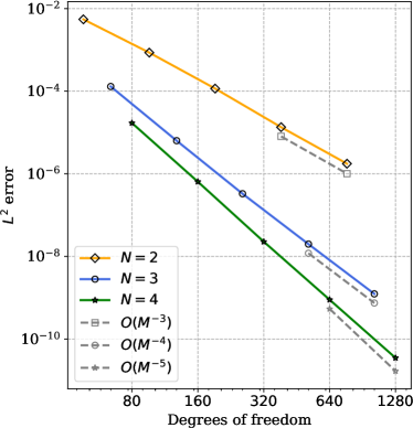
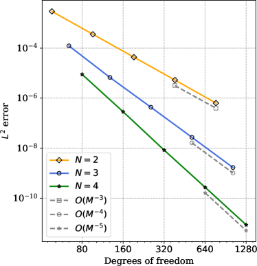
(a)	(b)

Figure 1: Error convergence analysis of a smooth test with source terms for (a) $\rho$, (b) $p_{11}$ variable

4.2 Riemann problems

Here, we test the scheme on Riemann problems in the absence of source terms. The domain is $\Omega=[-0.5,0.5]$. The first problem is Sod’s test

$$(\rho,v_{1},v_{2},p_{11},p_{12},p_{22})=\begin{cases}(1,0,0,2,0.05,0.6),\qquad&x<0\\ (0.125,0,0,0.2,0.1,0.2),&x>0\end{cases}$$

The second is a problem from Meena_Kumar_Chandrashekar_2017 with two rarefaction waves containing both low-density and low-pressure, leading to a near vacuum solution

$$\left(\rho,v_{1},v_{2},p_{11},p_{12},p_{22}\right)=\begin{cases}(1,-5,0,2,0,2),\qquad&x<0\\ (1,5,0,2,0,2),&x>0\end{cases}$$

The scheme is able to maintain admissibility in the near vacuum test and the results for both Riemann problems are shown in Figure 2 where convergence is seen under grid refinement.

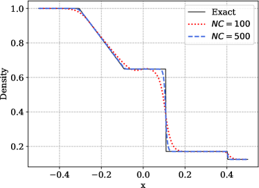
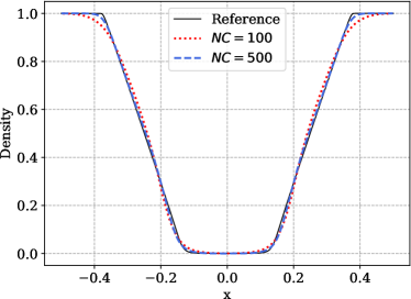
(a)	(b)

Figure 2: Density plots of numerical solutions with polynomial degree $N=2$ for (a) Sod’s problem, (b) Two rarefaction (near vacuum) problem

4.3 Shu-Osher test

This is a modified version of the standard Shu-Osher test, taken from Meena2020 . The primitive variables $\boldsymbol{V}=(\rho,v_{1},v_{2},p_{11},p_{12},p_{22})$ are initialized in domain $[-5,5]$ as

$$\boldsymbol{V}=\begin{cases}(3.857143,2.699369,0,10.33333,0,10.33333),\qquad&\text{if }x\leq-4\\ (1+0.2\sin(5x),0,0,1,0,1),&\text{if }x>-4\end{cases}$$

The simulation is performed with polynomial degree $N=4$ using 200 elements and run till time $t=1.8$ and the results with both blending and TVB limiter are shown in Figure 3 where, as expected, the blending limiter is giving much better resolution of the shock and high-frequency wave.

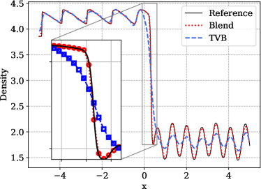
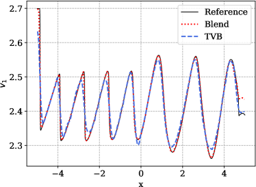
(a)	(b)

Figure 3: Numerical solution for Shu-Osher problem with polynomial degree $N=4$ using TVB and blending limiter and we show (a) Density, (b) $v_{1}$ profiles. The density plot has an inset plot near the shock which compares number of cells smeared across the shock by blending and TVB limiter.

4.4 Two dimensional near vacuum test

This is a near vacuum test taken from Meena_Kumar_Chandrashekar_2017 , and is thus another verification of our admissibility preserving framework. The domain is $\Omega=[-1,1]^{2}$ with outflow boundary conditions. The initial conditions are

$$\begin{gathered}{\rho}=1,\quad{p_{11}}={p_{22}}=1,\quad{p_{12}}=0,\quad{v_{1}}=8f_{\textrm{s}}(r)\cos{\theta},\quad{v_{2}}=8f_{\textrm{s}}(r)\sin{\theta}\end{gathered}$$

where $r=\sqrt{x^{2}+y^{2}}$, $\theta=\arctan(y/x)\in[-\pi,\pi]$ and $s=0.06\Delta x$ for mesh size $\Delta x(=\Delta y)$ of the uniform mesh. The $f_{s}(r)$ smoothens the velocity profile near the origin as $\theta$ is not defined there

$$f_{s}(r)=\begin{cases}-2\left(\frac{r}{s}\right)^{3}+3\left(\frac{r}{s}\right)^{2},\quad&\operatorname{if}r<s\\ 1,&\text{otherwise}\end{cases}$$

The numerical solution computed using polynomial degree $N=2$ and 100 elements is shown at the time $t=0.02$. The results are shown in Figure 4 and are similar to those seen in the literature.

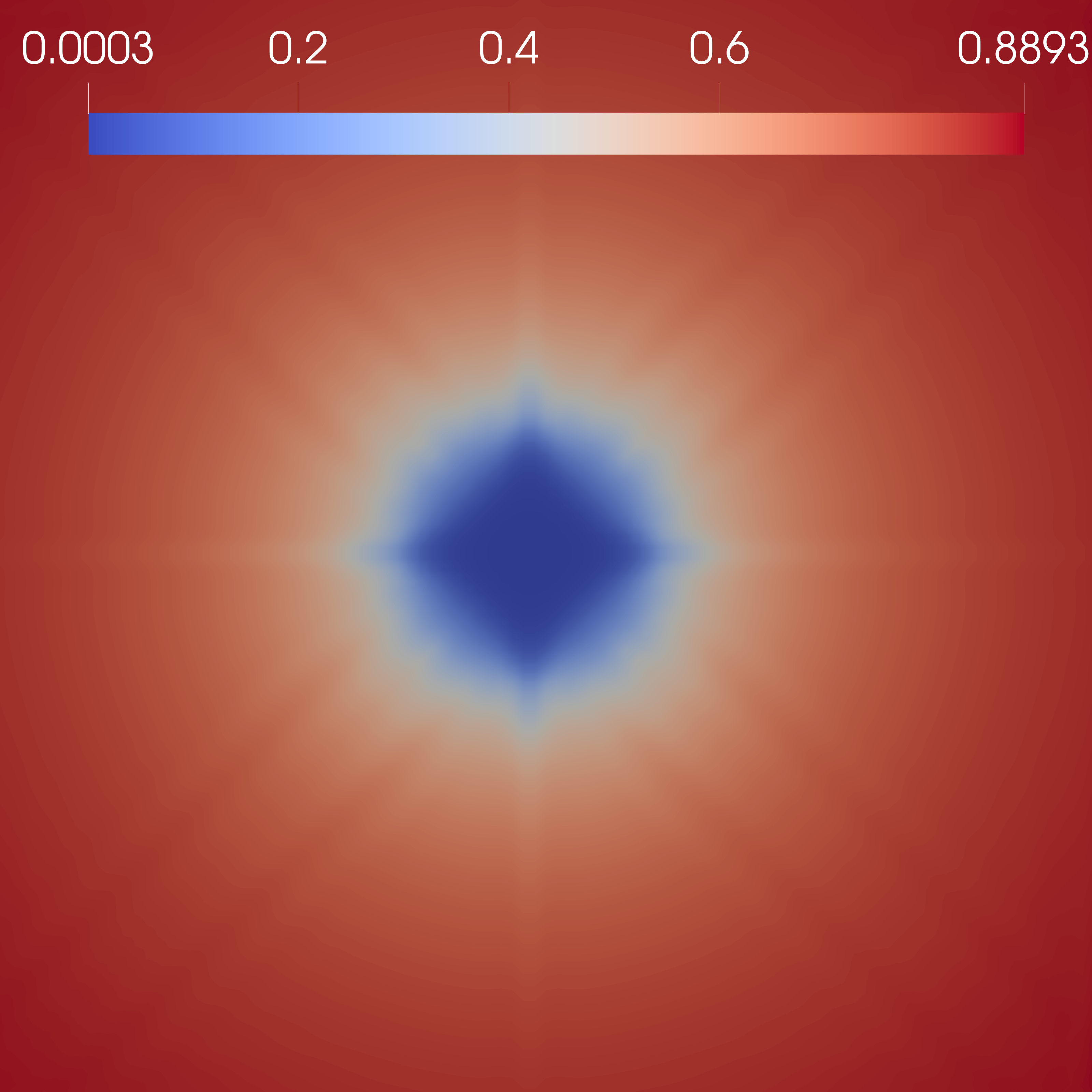
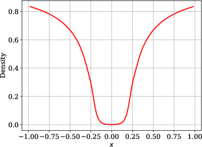
(a)	(b)

Figure 4: 2-D near vacuum test. Density plot of numerical solution with degree $N=2$ on a $100^{2}$ element mesh (a) Pseudocolor plot (b) Solution cut along the line $y=0$

4.5 Realistic simulation

Consider the domain $\Omega=[0,100]^{2}$ with outflow boundary conditions. The uniform initial condition is taken to be

$$\rho=0.109885,\quad v_{1}=v_{2}=0,\quad p_{11}=p_{22}=1,\quad p_{12}=0$$

with the electron quiver energy $W(x,y,t)=\exp(-0.01((x-50)^{2}+(y-50)^{2}))$. The source term is taken from Berthon2015 , and only has the $x$ component, i.e, $\boldsymbol{s}^{y}\left(\boldsymbol{u}\right)=\boldsymbol{0}$, even though $W$ continues to depend on $x$ and $y$. An additional source corresponding to energy components $\boldsymbol{s}_{E}=(0,0,0,\nu_{T}\rho W,0,0)$ is also added where $\nu_{T}$ is an absorption coefficient. Thus, the source terms are $\boldsymbol{s}=\boldsymbol{s}_{x}+\boldsymbol{s}_{E}$. The simulation is run till $t=0.5$ on a grid of 100 cells. The blending limiter from babbar2023admissibility was used in this test as it captured the smooth extrema better. The density plot with a cut at $y=4$ is shown in Figure 5.

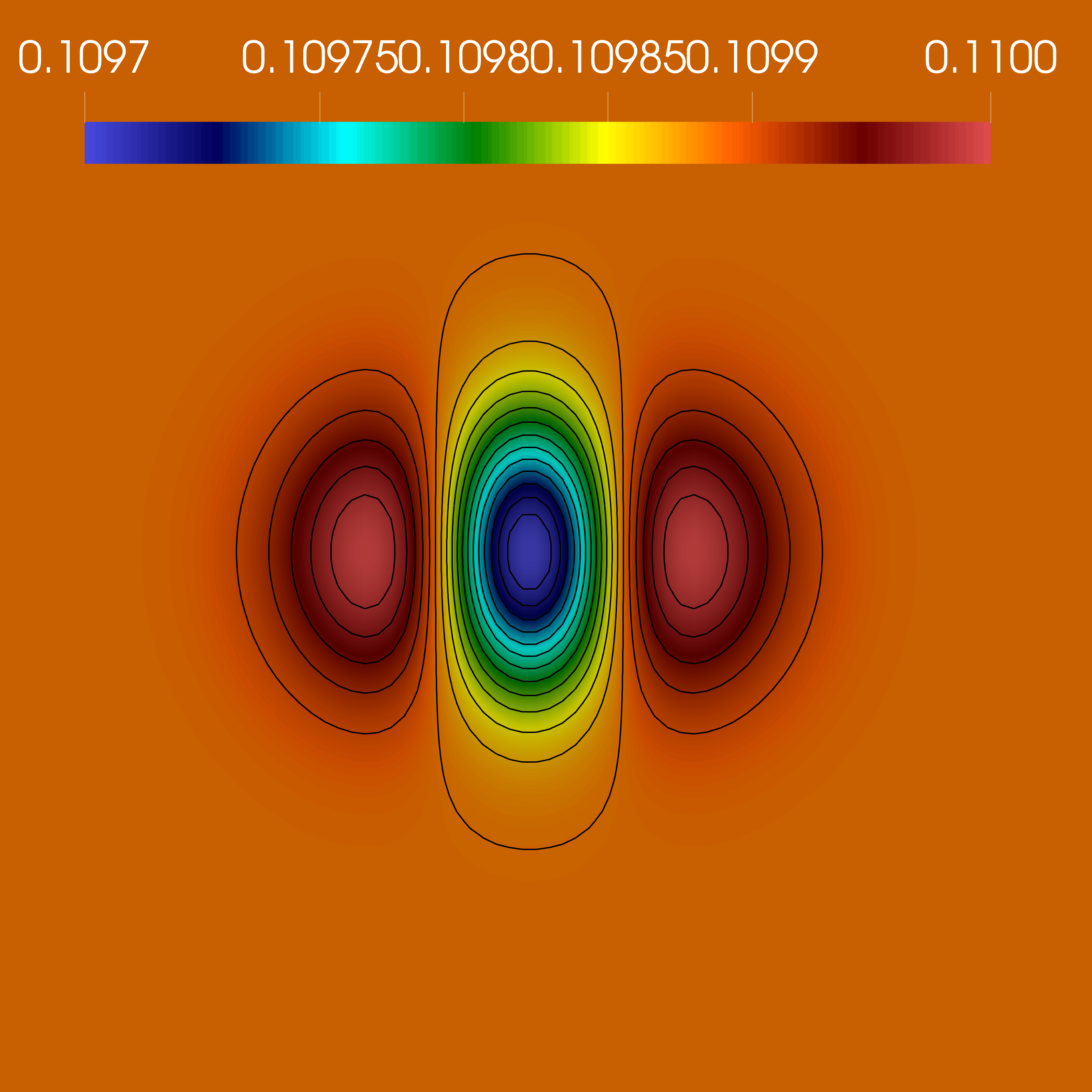
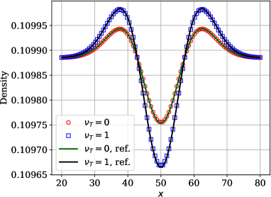
(a)	(b)

Figure 5: Realistic simulation. Density profile computed with degree $N=4$ on $100^{2}$ element mesh. (a) Pseudocolor color plot (b) Cut at $y=4$ comparing different absorption coefficient $\nu_{T}$.

5 Conclusions

A generalized framework was developed for high order admissibility preserving Lax-Wendroff (LW) schemes. The framework is a generalization of babbar2023admissibility as it is independent of the shock capturing scheme used and can, in particular, be used without the subcell based limiter of babbar2023admissibility . The framework was also shown to be an extension of Zhang2010b to LW. The LW scheme was extended to be applicable to problems with source terms while maintaining high order accuracy. Provable admissibility preservation in presence of source terms was also obtained by limiting the time average sources. The claims were numerically verified on the Ten Moment problem model where the scheme showed high order accuracy and robustness.

References

- (1) A. Babbar and P. Chandrashekar, Admissibility preservation for Ten moment problem with Tenkai.jl. https://github.com/Arpit-Babbar/tenkai-icosahom2023, 2024.
- (2) A. Babbar, P. Chandrashekar, and S. K. Kenettinkara, Tenkai.jl: Temporal discretizations of high-order PDE solvers. https://github.com/Arpit-Babbar/Tenkai.jl, 2023.
- (3) A. Babbar, S. K. Kenettinkara, and P. Chandrashekar, Lax-wendroff flux reconstruction method for hyperbolic conservation laws, Journal of Computational Physics, (2022), p. 111423.
- (4) , Admissibility preserving subcell limiter for lax-wendroff flux reconstruction, Springer Journal of Scientific Computing, (2024). Accepted for publication.
- (5) C. Berthon, Numerical approximations of the 10-moment gaussian closure, Mathematics of Computation, 75 (2006), p. 1809–1831.
- (6) C. Berthon, B. Dubroca, and A. Sangam, An entropy preserving relaxation scheme for ten-moments equations with source terms, Communications in Mathematical Sciences, 13 (2015), p. 2119–2154.
- (7) B. Biswas, H. Kumar, and A. Yadav, Entropy stable discontinuous galerkin methods for ten-moment gaussian closure equations, Journal of Computational Physics, 431 (2021), p. 110148.
- (8) R. Bürger, S. K. Kenettinkara, and D. Zorío, Approximate Lax–Wendroff discontinuous Galerkin methods for hyperbolic conservation laws, Computers & Mathematics with Applications, 74 (2017), pp. 1288–1310.
- (9) A. Cicchino, S. Nadarajah, and D. C. Del Rey Fernández, Nonlinearly stable flux reconstruction high-order methods in split form, Journal of Computational Physics, 458 (2022), p. 111094.
- (10) B. Cockburn, G. E. Karniadakis, C.-W. Shu, M. Griebel, D. E. Keyes, R. M. Nieminen, D. Roose, and T. Schlick, eds., Discontinuous Galerkin Methods: Theory, Computation and Applications, vol. 11 of Lecture Notes in Computational Science and Engineering, Springer Berlin Heidelberg, Berlin, Heidelberg, 2000.
- (11) M. Dumbser, D. S. Balsara, E. F. Toro, and C.-D. Munz, A unified framework for the construction of one-step finite volume and discontinuous Galerkin schemes on unstructured meshes, Journal of Computational Physics, 227 (2008), pp. 8209–8253.
- (12) S. Hennemann, A. M. Rueda-Ramírez, F. J. Hindenlang, and G. J. Gassner, A provably entropy stable subcell shock capturing approach for high order split form dg for the compressible euler equations, Journal of Computational Physics, 426 (2021), p. 109935.
- (13) H. T. Huynh, A Flux Reconstruction Approach to High-Order Schemes Including Discontinuous Galerkin Methods, Miami, FL, June 2007, AIAA.
- (14) P. Lax and B. Wendroff, Systems of conservation laws, Communications on Pure and Applied Mathematics, 13 (1960), pp. 217–237.
- (15) C. D. Levermore, Moment closure hierarchies for kinetic theories, Journal of Statistical Physics, 83 (1996), p. 1021–1065.
- (16) S. Lou, C. Yan, L.-B. Ma, and Z.-H. Jiang, The Flux Reconstruction Method with Lax–Wendroff Type Temporal Discretization for Hyperbolic Conservation Laws, Journal of Scientific Computing, 82 (2020), p. 42.
- (17) A. K. Meena and H. Kumar, Robust MUSCL Schemes for Ten-Moment Gaussian Closure Equations with Source Terms, International Journal on Finite Volumes, (2017).
- (18) A. K. Meena, H. Kumar, and P. Chandrashekar, Positivity-preserving high-order discontinuous galerkin schemes for ten-moment gaussian closure equations, Journal of Computational Physics, 339 (2017), p. 370–395.
- (19) A. K. Meena, R. Kumar, and P. Chandrashekar, Positivity-preserving finite difference weno scheme for ten-moment equations with source term, Journal of Scientific Computing, 82 (2020).
- (20) J. Qiu, M. Dumbser, and C.-W. Shu, The discontinuous Galerkin method with Lax–Wendroff type time discretizations, Computer Methods in Applied Mechanics and Engineering, 194 (2005), pp. 4528–4543.
- (21) J. Qiu and C.-W. Shu, Finite Difference WENO Schemes with Lax–Wendroff-Type Time Discretizations, SIAM Journal on Scientific Computing, 24 (2003), pp. 2185–2198.
- (22) A. Rueda-Ramírez and G. Gassner, A subcell finite volume positivity-preserving limiter for DGSEM discretizations of the euler equations, in 14th WCCM-ECCOMAS Congress, CIMNE, 2021.
- (23) V. A. Titarev and E. F. Toro, ADER: Arbitrary High Order Godunov Approach, Journal of Scientific Computing, 17 (2002), pp. 609–618.
- (24) W. Trojak and F. D. Witherden, A new family of weighted one-parameter flux reconstruction schemes, Computers & Fluids, 222 (2021), p. 104918.
- (25) P. E. Vincent, P. Castonguay, and A. Jameson, A New Class of High-Order Energy Stable Flux Reconstruction Schemes, Journal of Scientific Computing, 47 (2011), pp. 50–72.
- (26) X. Zhang and C.-W. Shu, On maximum-principle-satisfying high order schemes for scalar conservation laws, Journal of Computational Physics, 229 (2010), pp. 3091–3120.
- (27) X. Zhang and C.-W. Shu, On positivity-preserving high order discontinuous galerkin schemes for compressible euler equations on rectangular meshes, Journal of Computational Physics, 229 (2010), pp. 8918–8934.
- (28) D. Zorío, A. Baeza, and P. Mulet, An Approximate Lax–Wendroff-Type Procedure for High Order Accurate Schemes for Hyperbolic Conservation Laws, Journal of Scientific Computing, 71 (2017), pp. 246–273.