Frenetix Motion Planner: High-Performance and Modular Trajectory Planning Algorithm for Complex Autonomous Driving Scenarios

Abstract

Our work aims to present a high-performance and modular sampling-based trajectory planning algorithm for autonomous vehicles. This algorithm is tailored to address the complex challenges in solution space construction and optimization problem formulation within the path planning domain. Our method employs a multi-objective optimization strategy for efficient navigation in static and highly dynamic environments, focusing on optimizing trajectory comfort, safety, and path precision. This algorithm was then used to analyze the algorithm performance and success rate in 1750 virtual complex urban and highway scenarios. Our results demonstrate fast calculation times (8ms for 800 trajectories), a high success rate in complex scenarios (88%), and easy adaptability with different modules presented. The most noticeable difference exhibited was the fast trajectory sampling, feasibility check, and cost evaluation step across various trajectory counts. While our study presents promising results, it’s important to note that our assessments have been conducted exclusively in simulated environments, and real-world testing is required to fully validate our findings. The code and the additional modules used in this research are publicly available as open-source software and can be accessed at the following link: https://github.com/TUM-AVS/Frenetix-Motion-Planner.

I Introduction

With its promise of revolutionizing transportation, autonomous driving technology faces significant real-world challenges brought to light through various collision reports and practical experiences [1]. Among these challenges are the complexities of urban navigation, the unpredictability of traffic and pedestrian behavior, and the necessity for rapid, informed decision-making in ever-changing environments [2]. These factors underscore the importance of high-performance and adaptable trajectory planning algorithms in autonomous vehicles (AVs) (Fig. 1). Unfortunately, foundational, traditional trajectory planning methods often struggle to cope with the dynamic and intricate nature of real-world driving scenarios, especially in diverse and unpredictable conditions encountered in urban settings. This highlights the need for trajectory planning algorithms with low calculation times, robustness, and high adaptability to various situations to ensure safety and efficiency in autonomous driving. Our work introduces an advanced analytical sampling-based trajectory planning algorithm to address these challenges. This algorithm is designed to efficiently handle the complexities and uncertainties inherent in urban driving environments. In summary, this work has three main contributions:

• We present a publicly available sampling-based trajectory planner for AVs called FRENETIX, employing a multi-objective optimization strategy for efficient navigation in complex environments, focusing on optimizing trajectory comfort, safety, and path precision. Unlike anything available before, we offer an out-of-the-box method integrated into the simulation environment with a wide variety of scenarios.

• We provide a modular approach to improve adaptability and scalability, allowing for easy integration and optimal functionality of each component within the system, catering to a wide range of scenarios.

• We provide a Python and C++ implementation to demonstrate the algorithm’s real-time capability and success rate in complex scenarios, showcasing its potential effectiveness and efficiency for real-world applications.

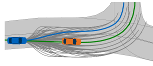
Figure 1: Visualization of a trajectory planner for AVs, depicting potential trajectories while selecting an optimal trajectory for safe navigation in a dynamic and complex urban environment.

II Related Work

Motion planning is a critical component in the software development of autonomous vehicles [3]. Motion planners operate on a specific time horizon and attempt to avoid obstacles while quickly generating an efficient and reliable local trajectory. The trajectory includes both a path ($x(t)$, $y(t)$ - position) and a velocity profile $v(t)$, which provide the reference information for subsequent lateral and longitudinal control. This task is complex due to dynamic and unpredictable road environments, especially in urban settings with static and dynamic obstacles like pedestrians and other vehicles [4]. Several concepts have been developed from various theoretical foundations in recent decades [5, 6]. Optimization methods [7, 8, 9], like optimal control problems (OCP), are known for their mathematical rigor and ability to optimize continuous paths, often leveraging calculus of variations to find smooth trajectories in complex spaces. These methods focus on finding the best solution or path under a given set of constraints and use mathematical optimization techniques to minimize or maximize an objective function. These algorithms can provide optimal solutions under certain conditions but may be computationally intensive and less effective in highly dynamic or unpredictable environments. Graph-based methods  [6, 5, 10] discretize the planning space into nodes and edges, symbolizing possible vehicle positions and paths. This approach is valid in structured and well-known environments like road networks. This enables efficient path planning through well-established graph algorithms. Unfortunately, these algorithms can be limited by the accuracy of the graph representation and may not handle dynamic obstacles well. Sampling-based methods  [11, 12, 13, 14] have gained popularity for their effectiveness in high-dimensional spaces. These methods randomly search the free space around the vehicle’s current state for target states. Once an available target state is found, a trajectory is created which connects the current driving state of the vehicle to the selected target state. By introducing randomness, these algorithms are generally efficient but do not provide guarantees for finding an optimal trajectory. AI-based methods [15, 16] introduce learning techniques, often utilizing neural networks or machine learning algorithms to adapt and improve planning strategies based on past experiences (data or predictions) or simulated scenarios. These algorithms can adapt to new situations, learn from experience, and behave more effectively in dynamic and unpredictable environments. Unfortunately, they require a substantial amount of data for training and may be less interpretable. Finally, hybrid methods combine the strengths of various approaches and blending techniques like graph-based and sampling methods to create robust solutions that can adapt to a wide range of planning challenges.

III Methodology

This section introduces the FRENETIX algorithm, a motion planning algorithm for AVs. FRENETIX enables efficient, safe, and reliable navigation (e.g., overtaking), especially in dynamic and complex environments. The modular structure of FRENETIX is a key feature, simplifying the planning process while enhancing adaptability and scalability for different scenarios. Developed using Python for its flexibility and prototyping capabilities, FRENETIX also incorporates C++ components to enhance computational efficiency. This combination results in a system that optimizes performance and is practical for deployment. At its heart is an iterative motion planning cycle, including cost functions, risk assessments, validity checks, and safety features for continuously refining the vehicle’s trajectory in response to environmental changes, as depicted in Fig. 2.

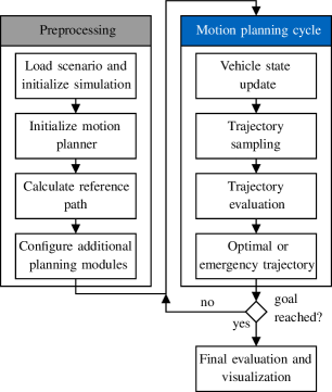
Figure 2: FRENETIX motion planning architecture.

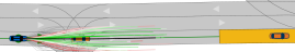
(a)

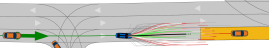
(b)

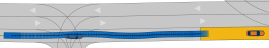
(c)

Figure 3: Visualization of the sequential progression of the motion planning algorithm over time. The black trajectory shows the selected optimal trajectory. The gray trajectories are kinematically infeasible. The feasible trajectories are highlighted using a color scale corresponding to the cost, where green indicates a low cost and red indicates a high cost.

III-A Preprocessing

The motion planning algorithm obtains the environment data from the simulation environment, in our case, from the CommonRoad [17] scenario database (Fig. 3). The environment, modeled as a semantic lanelet network with static and dynamic obstacles and traffic signs, contains traffic participant data, regulatory elements, and the specific planning problem. Each obstacle is characterized by its type, dimensions, location, and orientation. The planning problem is defined by the initial state of the ego vehicle and the conditions required to reach a specific goal. An optimal global route through the lanelet network is needed to form a reference path $\Gamma$ for subsequent trajectory generation in the Frenet coordinate system. To select the optimal sequence of lanelets, a graph optimization algorithm, such as Dijkstra [18] or A* [19], is employed. The selected lanelets are interconnected through their centroids, forming a navigable route. Since FRENETIX has a modular approach, one is capable of initializing further FRENETIX modules to expand the planner’s capabilities, for example:

• Vehicle motion prediction [20]

• Risk assessment and harm estimation [21, 22]

• Occlusion-aware trajectory planning [23]

• Multi-agent simulation framework

• Behavior planning extension

III-B Motion Planning Cycle

Vehicle state update: The motion planning cycle starts by updating the ego vehicle’s state in our trajectory planning algorithm. This involves refreshing the state vector with the latest position and motion data and merging past states with current planner-directed controls.

Trajectory sampling: Our planner is implemented as a semi-reactive approach [12] to generate vehicle trajectories by continuously optimizing local paths and performing cyclic replanning steps (Fig. 3b). Samples are generated in the Frenet coordinate system to simplify trajectory planning by separating longitudinal and lateral vehicle motion. The vehicle’s position in the Frenet frame is quantified using two key parameters: the lateral displacement, denoted as $d$, and the longitudinal displacement, represented by $s$, as illustrated in Fig. 4 [12]. Unlike the traditional Cartesian coordinate system, the Frenet coordinate system adopts a path-focused methodology. Within this system, a vehicle’s position and movement are characterized by their relationship to a predetermined reference path, providing a distinct, path-oriented viewpoint.

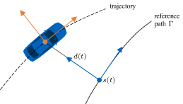
Figure 4: Frenet coordinate system for trajectory generation, adapted from [11].

The trajectory planning algorithm generates potential final states for lateral and longitudinal trajectories within a predetermined discretization scheme shown in Table I.

TABLE I: Sampling matrix.

Sampling category	Sampling scheme
time-sampling	$[t_{\text{min}},t_{1},t_{2},...,t_{\text{max}}]$
d-sampling	$[d_{\text{min}},d_{1},...,d_{\text{curr}},d_{\text{curr}+1},...,d_{\text{max}}]$
velocity-sampling	$[v_{\text{min}},v_{1},...,v_{\text{curr}},v_{\text{curr}+1},...,v_{\text{max}}]$
s-sampling	$[s_{\text{curr}},s_{1},s_{2},...,s_{\text{max}}]$

The density and number of trajectories can be defined. $t_{\text{max}}$ corresponds to the maximum sampled time horizon $\tau$ and the index $curr$ represents a clipping to the current ego vehicle state. All trajectories are extended to a fixed planning horizon $T$ to ensure comparability between all samples for later cost evaluations. $v_{\text{min}}$ and $v_{\text{max}}$ are dependent on the current vehicle state and the acceleration limits. Due to the dependencies, the s-sampling method is only used if velocity-sampling is deactivated. This is because the longitudinal end state can only be defined by the velocity or position range to avoid overdetermination. The sampling scheme in Table I contains the possible variants and the number of trajectories to be generated. There are extensions to the systematic sampling procedure, e.g., limiting sampling to the width of the roadway or the reachable set of the ego vehicle [24]. For lateral trajectories, the sampling process involves considering different lateral distances $d_{\mathrm{\tau}}$ from the reference path $\Gamma$ and distinct time horizons $\tau$. Similarly, for longitudinal trajectories, the algorithm samples endpoints at various velocities $v_{\mathrm{\tau}}$ and again distinct time horizons. Alternatively, the endpoint $s_{\mathrm{\tau}}$ can be defined directly over all sampled time horizons $\tau$. In this case, the velocity profile is adapted to the endpoint constraint. This method ensures that the longitudinal trajectory samples represent different speeds and acceleration profiles. These sampled final states serve as targets for the vehicle to conclude its trajectory. To effectively connect an initial state $\zeta(0)=\zeta_{\mathrm{0}}$ with a final state $\zeta(\tau)=\zeta_{\mathrm{\tau}}$ and form a coherent path, suitable polynomial functions are employed (Fig. 3c). In lateral motion planning, quintic polynomial functions are utilized to guarantee a trajectory that is both smooth and minimal in jerk [25]. Consequently, the trajectory along the lateral direction is represented by a polynomial function of the form:

$$\zeta(t)=c_{\mathrm{0}}+c_{\mathrm{1}}\,t+c_{\mathrm{2}}\,t^{2}+c_{\mathrm{3}}\,t^{3}+c_{\mathrm{4}}\,t^{4}+c_{\mathrm{5}}\,t^{5}$$ (1)

Differentiating the polynomial function (Eq. 1) twice yields a system of equations as follows:

$$\begin{bmatrix}\zeta(t)\\ \dot{\zeta}(t)\\ \ddot{\zeta}(t)\\ \end{bmatrix}=\begin{bmatrix}1&t&t^{2}&t^{3}&t^{4}&t^{5}\\ 0&1&2t&3t^{2}&4t^{3}&5t^{4}\\ 0&0&2&6t&12t^{2}&20t^{3}\\ \end{bmatrix}\begin{bmatrix}c_{0}\\ c_{1}\\ c_{2}\\ c_{3}\\ c_{4}\\ c_{5}\\ \end{bmatrix}$$ (2)

This matrix equation establishes the relationship between the polynomial coefficients $c_{0},\ldots,c_{5}$ and the vehicle’s state. In the case of the lateral movement, the boundary conditions for solving $c_{0},\ldots,c_{5}$ are set as follows [11]:

$$\zeta(t=0) =d_{0}, \zeta(t=\tau) =d_{\mathrm{\tau}},$$ (3)

$$\dot{\zeta}(t=0) =\dot{d}_{0}, \dot{\zeta}(t=\tau) =\dot{d}_{\mathrm{\tau}}=0,$$

$$\ddot{\zeta}(t=0) =\ddot{d}_{0}, \ddot{\zeta}(t=\tau) =\ddot{d}_{\mathrm{\tau}}=0.$$

The final lateral state velocity $\dot{d}_{\mathrm{\tau}}$ and acceleration $\ddot{d}_{\mathrm{\tau}}$ are set to zero, as the planning algorithm aims for a movement parallel to the reference path. For trajectory generation in the longitudinal direction, quartic polynomials are employed, providing an adequate description of vehicle motions in the longitudinal direction while ensuring minimal jerk [11]. When s-sampling is enabled, quintic polynomials are used because the endpoint manifold is omitted. The quartic polynomials in the longitudinal direction enable a manifold of the end positions since the velocity at the endpoint is not zero, while the acceleration is. The coefficients can analogously be calculated by solving an adapted version of Eq. 3 and applying the appropriate boundary conditions presented in [11]. By sampling $m$ trajectories in the longitudinal direction and $n$ in the lateral direction, a set comprising $m\times n$ trajectories is constructed through a systematic crosswise superposition of these two sets. The number of trajectories generated depends on the sampling scheme and density. With the completion of the sampling process, the trajectory samples are transformed back into global cartesian coordinates for further evaluation steps. The sampling process is visualized in  Fig. 5, where the resulting samples are shown in curvilinear and cartesian coordinate systems.

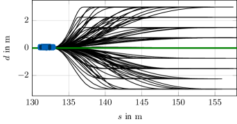
(a)

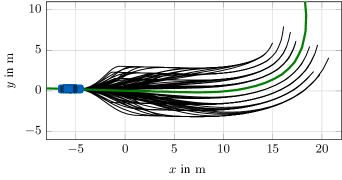
(b)

Figure 5: Sampling process in different coordinate systems, as per [12]: subfigure (a) illustrates trajectories in curvilinear coordinates, capturing the primary direction of movement within a curved reference frame. Subfigure (b) translates these trajectories into cartesian coordinates. The ego vehicle is blue ( ), indicating its position following the sampled trajectories along the reference path ( ).

Trajectory evaluation: The trajectory evaluation stage is required to assess the trajectory samples w.r.t. feasibility and optimality. Illustrated in Fig. 6, this stage adopts a systematic funnel approach, processing all trajectory samples generated in the preceding step through a sequence of evaluations. These assessments are designed to identify the optimal trajectory that the vehicle should adhere to for the subsequent timestep.

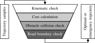
Figure 6: Trajectory evaluation: The selection funnel to find a cost-optimal and collision-free trajectory consists of four individual steps.

1.) Kinematic check: The first step in the evaluation process is a kinematic check. This involves assessing each trajectory sample to ensure it satisfies the kinematic constraints of the vehicle based on a kinematic single-track model. This step ensures that the trajectories are within the physical movement capabilities of the ego vehicle, considering the acceleration, curvature, curvature rate, and yaw rate. The permissible acceleration $a_{\text{permissible}}(t)$ is expressed as [17]:

$$a_{\text{permissible}}(t)=\begin{cases}a_{\text{max}}\cdot\frac{v_{\text{switch}}}{v(t)}&\text{if }v(t)>v_{\text{switch}}\\ a_{\text{max}}&\text{if }v(t)\leq v_{\text{switch}}\end{cases}$$ (4)

Let $v(t)$ denote the vehicle’s velocity at any point along the trajectory, and $a(t)$ represent the corresponding acceleration. Given a predefined maximum acceleration $a_{\text{max}}$ and a threshold velocity $v_{\text{switch}}$, which delineates the transition from constant to variable acceleration limits. The kinematic feasibility is thus determined by evaluating whether the actual acceleration $a(t)$ for each trajectory point remains within the bounds of $-a_{\text{max}}$ and $a_{\text{permissible}}(t)$:

$$-a_{\text{max}}\leq a(t)\leq a_{\text{permissible}}(t),\quad\forall t\in[t_{0},t_{f}]$$ (5)

Here, $t_{0}$ and $t_{f}$ represent the start and end of the considered time interval, respectively. Furthermore, the curvature $\kappa(t)$ of the trajectory at any point in time must not exceed the maximum curvature $\kappa_{\text{max}}$, which is derived from the maximum allowable steering angle $\delta_{\text{max}}$ and the wheelbase $L$ of the vehicle:

$$\kappa_{max}=\frac{\tan(\delta_{max})}{L}$$ (6)

Thus, the curvature constraint can be stated according to Eq. 7.

$$|\kappa(t)|\leq\kappa_{max},\quad\forall t\in[t_{0},t_{f}]$$ (7)

TABLE II: Implemented Cost Functions.

	Cost function	Formula	Explanation
	Acceleration	$J_{\mathrm{A}}=\int_{t_{\mathrm{0}}}^{t_{\mathrm{f}}}a^{2}\mathrm{d}t$	quantifies the total squared acceleration $a$, penalizing large accelerations
	Jerk	$J_{\mathrm{J}}=\int_{t_{\mathrm{0}}}^{t_{\mathrm{f}}}\dot{a}^{2}\mathrm{d}t$	quantifies the total squared jerk $\dot{a}$, penalizing abrupt changes
	Lateral jerk	$J_{\mathrm{J_{\mathrm{lat}}}}=\int_{t_{\mathrm{0}}}^{t_{\mathrm{f}}}\dot{a}_{\mathrm{lat}}^{2}\mathrm{d}t$	quantifies the total squared lateral jerk $\dot{a}_{\mathrm{lat}}$, penalizing sudden changes in lateral acceleration
Comfort	Longitudinal jerk	$J_{\mathrm{J_{\mathrm{lon}}}}=\int_{t_{\mathrm{0}}}^{t_{\mathrm{f}}}\dot{a}_{\mathrm{lon}}^{2}\mathrm{d}t$	quantifies the total squared longitudinal jerk $\dot{a}_{\mathrm{lat}}$, penalizing sudden changes in longitudinal acceleration
. Efficiency	Velocity offset	$J_{\mathrm{VO}}=\int_{t_{\mathrm{s}}}^{t_{\mathrm{f}}}\absolutevalue{v(t)-v_{\mathrm{ref}}(t)}\,\mathrm{d}t\newline \phantom{bbbbbbb}+(v(t_{\mathrm{f}})-v_{\mathrm{ref}}(t))^{2}$	calculates the absolute velocity offset compared to a reference velocity $v_{\mathrm{ref}}(t)$ over a given period from $t_{\mathrm{s}}$ to $t_{\mathrm{f}}$, with an additional emphasis on the squared difference in velocity at the final time $t_{\mathrm{f}}$
	Dist. to ref. path	$J_{\mathrm{RP}}=\int_{t_{\mathrm{0}}}^{t_{\mathrm{f}}}{d}^{2}(t)\,\mathrm{d}t$	measures the total squared distance from the reference path, penalizing deviations from the desired path
	Dist. to obstacle	$J_{\mathrm{DO}}=\sum_{1}^{n}\int_{t_{\mathrm{0}}}^{t_{\mathrm{f}}}\frac{1}{\Delta x_{\mathrm{DO}}^{2}}\mathrm{d}t$	computes the sum of the inverse squared distances to obstacles $\Delta x_{\mathrm{DO}}$ for $n$ different obstacles
	Collision prob.	$J_{\mathrm{CP}}=\sum_{1}^{n}\int_{t_{\mathrm{0}}}^{t_{\mathrm{f}}}\int f(x,0,\Sigma_{\mathrm{rot}})\mathrm{d}x\,\mathrm{d}t$	calculates the total collision probability over time for $n$ obstacles by integrating the probability density function with a rotated covariance matrix $\Sigma_{\mathrm{rot}}$ across a spatial domain $x$
Safety	Collision prob. mahalanobis	$J_{\mathrm{CM}}=\sum_{1}^{n}\int_{t_{0}}^{t_{f}}\frac{1-\frac{t}{T}}{d_{\mathrm{M}}(u(t),v(t),\Sigma(t))}\,\mathrm{d}t$	calculates the collision probability for $n$ obstacles by integrating the inverse Mahalanobis distance $d_{\mathrm{M}}$ between the trajectory point $u(t)$ and each obstacle’s predicted position $v(t)$, with a linearly decreasing weight over $T$

The rate of change of the curvature $\dot{\kappa}(t)$ should also be bounded to ensure smooth transitions in steering. Therefore, we assume a maximum acceptable curvature rate $\dot{\kappa}_{max}$ to determine the trajectory’s feasibility, where

$$|\dot{\kappa}(t)|\leq\dot{\kappa}_{max},\quad\forall t\in[t_{0},t_{f}]$$ (8)

Finally, the yaw rate $\dot{\psi}(t)$, which represents the rate of change of the vehicle’s orientation $\psi$, should not exceed the maximum yaw rate $\dot{\psi}_{max}$ determined by $\kappa_{max}$ and the vehicle’s velocity $v(t)$:

$$\dot{\psi}_{max}(t)=\kappa_{max}\cdot v(t)$$ (9)

The yaw rate constraint is:

$$|\dot{\psi}(t)|\leq\dot{\psi}_{max}(t),\quad\forall t\in[t_{0},t_{f}]$$ (10)

Should any trajectory sample violate these constraints, it is deemed infeasible, signifying a deviation from the vehicle’s kinematic capabilities.

2.) Cost calculation: After the kinematic validation, each trajectory is assigned a cost based on a cost function. The cost computation for the trajectory planning algorithm is formulated as a weighted sum of various partial cost components, each quantifying distinct aspects of the trajectory’s quality. The total cost $J_{\mathrm{sum}}(\xi|f_{\xi})$ for a given trajectory $\xi\in\mathcal{T}$ is expressed as:

$$J_{\mathrm{sum}}(\xi|f_{\xi})=\sum_{i=1}^{n}\omega_{\mathrm{i}}\cdot J_{\mathrm{i}}(\xi)$$ (11)

where $J_{\mathrm{i}}(\xi)$ represents the $i^{th}$ cost function from the implemented set of cost functions. The weighting factor $\omega_{\mathrm{i}}$ indicates the relative importance of the corresponding cost component in the overall cost calculation. The cost functions encompass criteria such as comfort, efficiency, and particularly safety [26]. Safety is quantified primarily through collision probability costs, derived from predictive models of other traffic participants’ movements [20]. By estimating the likelihood of a collision based on these predicted trajectories, the algorithm assigns a cost that reflects the potential collision probability. Each cost function is designed to provide a robust indicator of the trajectory’s viability. An overview of all implemented cost functions is given in Table II. After the cost computation for each trajectory, they are sorted in ascending order of their respective costs, placing the most cost-effective trajectory at the forefront for further evaluation.

3.) Collision check: The sorted trajectories then undergo a collision check using the drivability checker [27]. This step analyzes the trajectories for collisions with static and dynamic objects. As trajectories are required to be free of collisions for all continuous times $t$, it is crucial to ensure collision avoidance not just at discrete steps but also between any two subsequent states $x_{1}=x(t_{1})$ and $x_{2}=x(t_{2})$, where $t_{1}\leq t_{2}$. Therefore, the collision checker uses an oriented bounding box (OBB) around the occupied spaces for two consecutive time steps. This approach makes it possible to ensure a continuous collision-free path within these intervals [27]. Initially, the first trajectory in the list is checked for collisions. If it is collision-free, the process stops. As the trajectories are already sorted according to their cost, we only need to find the first collision-free trajectory, significantly reducing the computation time for collision checking.

4.) Road boundary check: The final step involves a road boundary check, where only the first collision-free trajectory is initially evaluated for adherence to road boundaries. If it keeps the vehicle on the road, it is accepted; otherwise, the next trajectory is checked until one meets both non-collision and road adherence criteria.

Optimal trajectory: The output of this evaluation funnel is the optimal trajectory, which has successfully passed through all the assessment layers with the lowest associated costs while ensuring safety. This trajectory is deemed the most suitable for execution by the vehicle, balancing efficiency, safety, and comfort.

Emergency risk trajectory: If the evaluation does not result in an optimal trajectory, FRENETIX calculates an additional emergency trajectory. This is done by assessing the risk $R(\mathcal{\xi})$ of an unavoidable collision trajectory for the ego vehicle and the potential collision partner. The risk is defined by the maximum harm and the collision probability [21].

$$\begin{split}R(\mathcal{\xi})=\mathrm{max}(p(\mathcal{\xi})\cdot H(\mathcal{\xi}))\end{split}$$ (12)

Emergency stopping trajectory: In scenarios where calculating the minimum risk trajectory proves infeasible, for instance, when no prediction information is available, the system defaults to a stopping trajectory. To optimize the braking process and minimize braking distance, the vehicle maintains its current lateral distance ($\text{argmin}_{i}\,|d_{\text{curr}}-d_{\text{samp}_{d}[i]}|$) from the reference path. This approach is specifically designed to maximize the absorption of longitudinal negative acceleration during braking. Furthermore, only dynamically feasible trajectories $\mathcal{T}_{f}$ are considered in this process, ensuring both effectiveness and safety in vehicle maneuvering.

IV Results & Analysis

IV-A Environment & Evaluation

We evaluate our new FRENETIX motion planner in the CommonRoad simulation environment [17]. The AV has to find a trajectory in given scenarios to reach the goal region in a limited amount of time without a collision and in a kinematically feasible way. The algorithm’s success rate depends on many factors and the difficulty of the scenarios. We use $1750\text{\,}$ CommonRoad scenarios to evaluate the performance of the algorithm. In this evaluation, we maintain consistent settings and cost weightings for the algorithm, intentionally avoiding adjustments or fine-tuning. The results created are, therefore, from an untuned model lacking specialized behavior features, especially in edge-case scenarios. This ensures that the evaluation of performance is independent and unbiased. Fig. 7 shows the simulation results of the $1750\text{\,}$ scenarios.

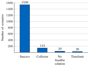
Figure 7: Scenario evaluation of 1750 CommonRoad scenarios.

Our FRENETIX planner finds in $1539\text{\,}$ scenarios a safe and valid solution and can solve the scenario. In $143\text{\,}$ scenarios, FRENETIX is causing a collision. It should be noted that incorrect predictions of vehicle movements and collisions, where the responsibility does not lie with the ego vehicle, cause around $40\text{\,}\mathrm{\char 37\relax}$ of the accidents. In $29\text{\,}$ scenarios, FRENETIX could not reach the goal within a given time limit.

IV-B Vehicle Dynamic Interaction Scenario

We evaluate FRENETIX in two detailed scenarios: an overtaking maneuver in Fig. 8 and an overtaking maneuver with an oncoming vehicle in Fig. 9. We use different cost weight settings displayed in Table III to investigate the trajectory selection process while overtaking.

TABLE III: Cost weight variations & planner setting for trajectory selection process.

Planner Settings	Values
Lateral jerk	$0.1\text{\,}$
Longitudinal jerk	$0.1\text{\,}$
Distance to reference path	$0.1\text{\,}$
Velocity	[$0.05\text{\,}$,$0.1\text{\,}$,$1.0\text{\,}$]
Distance to obstacles	[$0\text{\,}$,$100\text{\,}$]
Collision probability	[$2\text{\,}$,$100\text{\,}$,$1000\text{\,}$]
Planning horizon $T$	$3\text{\,}\mathrm{s}$
Max./Min. $d$-sampling	[$-3.5\text{\,}$,$3.5\text{\,}$]

The weightings depend on the respective cost function, meaning they can only be considered relative to their changes between different runs. In the following investigations, a distinction is made between the different weighting levels to demonstrate the performance and functionality of the algorithm. A detailed parameter analysis is not carried out, as this can be obtained from the literature [28]. In the first study without oncoming traffic, the costs of the collision probability are varied to investigate the change in driving behavior.

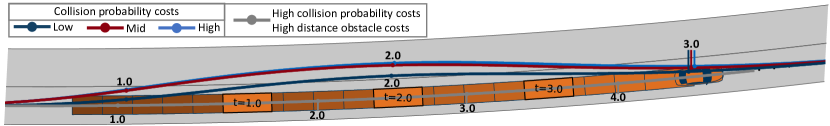
Figure 8: Overtaking scenario with four different cost-weight settings. The numbers next to the trajectories illustrate the progression of the runs in $\text{\,}\mathrm{s}$.

In our study, the overtaken vehicle maintains a constant speed of $13\text{\,}\mathrm{m}\text{\,}{\mathrm{s}}^{-1}$. As illustrated in Fig. 8, we observe that augmenting the costs associated with collision probability leads to an increased lateral distance from overtaking vehicle. If the distance is sufficient, the cost of the collision probability decreases so much that it hardly influences the distance so that the vehicle does not move unnecessarily far from the other vehicle. This ensures that the vehicle does not deviate excessively from its reference path. Under these conditions, the overtaking velocity is influenced by the target speed. Conversely, when the costs for increased distance to an obstacle are factored in, the ego vehicle stays behind the preceding vehicle instead of overtaking. This is due to the increased distance to obstacle costs to the leading vehicle, which exceeds the velocity. The trajectory planner can also manage critical situations with conflicting objectives. Fig. 9 shows the same scenario with an oncoming vehicle. The study examines the variation in velocity costs and how to handle the oncoming traffic. The velocity costs are dependent on the target speed. With high velocity costs, the vehicle accelerates significantly faster and can turn in again sooner after overtaking. With low velocity costs, the vehicle in front cannot be overtaken in time. The ego vehicle has to pull in again and overtake at a later timestep after $5\text{\,}\mathrm{s}$. Nevertheless, none of the different setups results in a collision with the other vehicles. However, if we deactivate one of the two important cost functions, the vehicle fails. Collision probability costs and velocity costs are necessary to achieve the goal region.

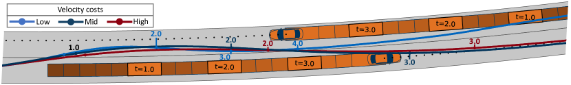
Figure 9: Overtaking scenario with an oncoming vehicle with three different cost-weight settings. The numbers next to the trajectories illustrate the progression of the runs in $\text{\,}\mathrm{s}$.

IV-C Calculation time

To analyze computation times for trajectory planning, the study utilized a Dell Alienware computer equipped with an AMD 7950X processor, 128 GB RAM, and an NVIDIA GeForce RTX 4090 graphics card. We benchmark our FRENETIX C++ implementation against a FRENETIX Python implementation. We distinguish between single-core (SC) and multiprocessing (MP) since sampling-based planners are easy to parallelize. Since we are using a sampling scheme, we cannot raise the number of trajectories linearly. We investigate how much time the algorithm needs to create the trajectory samples, check the feasibility of each trajectory, and calculate their costs. We depict the results of this evaluation in Table IV.

TABLE IV: Calculation times (in milliseconds) for trajectory sampling, feasibility check, and cost evaluation.

Trajectories	C++ (SC)	C++ (MP)	% Difference (SC/MP)	Python (SC)	Python (MP)	% Difference (SC/MP)
50	$4.68\text{\,}\mathrm{ms}$	$3.29\text{\,}\mathrm{ms}$	147.72%	$35.68\text{\,}\mathrm{ms}$	$124.67\text{\,}\mathrm{ms}$	28.62%
180	$7.98\text{\,}\mathrm{ms}$	$3.92\text{\,}\mathrm{ms}$	203.57%	$124.69\text{\,}\mathrm{ms}$	$133.62\text{\,}\mathrm{ms}$	93.32%
800	$29.37\text{\,}\mathrm{ms}$	$7.87\text{\,}\mathrm{ms}$	373.73%	$457.87\text{\,}\mathrm{ms}$	$214.72\text{\,}\mathrm{ms}$	213.24%
3500	$97.94\text{\,}\mathrm{ms}$	$29.82\text{\,}\mathrm{ms}$	328.44%	$1667.42\text{\,}\mathrm{ms}$	$590.36\text{\,}\mathrm{ms}$	282.44%
13000	$661.74\text{\,}\mathrm{ms}$	$112.38\text{\,}\mathrm{ms}$	588.84%	$5912.78\text{\,}\mathrm{ms}$	$1819.21\text{\,}\mathrm{ms}$	325.02%
90000	$5520.05\text{\,}\mathrm{ms}$	$717.05\text{\,}\mathrm{ms}$	769.83%	$44\,094.33\text{\,}\mathrm{ms}$	$10\,986.14\text{\,}\mathrm{ms}$	401.36%

The results reveal significant differences in calculation times between different implementations. The percentage differences between SC and MP modes were remarkably high, indicating a substantial efficiency gain in multi-processing. For instance, for $90\,000\text{\,}$ trajectories, the time was reduced from $5.52\text{\,}\mathrm{s}$ in SC to $0.717\text{\,}\mathrm{s}$ in MP. In the comparative analysis of Python implementations, MP exhibits a threshold-dependent efficacy. Specifically, Python-MP demonstrates a net advantage beyond a critical number of trajectories. This is attributable to the inherent overhead associated with MP under Python, which can outweigh the computational gains when dealing with a limited set of trajectories. Conversely, the C++ implementation showcases a more efficient resource utilization.

V Discussion

The results from our study indicate that the FRENETIX algorithm presented is effective in rapidly finding a safe and reliable trajectory in dynamic environments. The algorithm’s modular structure allows for quickly adapting and integrating new features and modules. However, it is essential to note that specific settings and parameters influence the algorithm’s performance, which is consistent with expectations for an analytical algorithm. During our research, collisions and other issues were mainly attributed to the lack of features for specific scenarios or inadequate parameter tuning. Nonetheless, the potential for optimizing vehicle behavior in various situations is achievable through further extensions. The cost functions demonstrate a variable influence on the target variables, facilitating the successful simulation of complex maneuvers, such as overtaking in the presence of oncoming traffic.

VI Conclusion & Outlook

In this paper, we introduced FRENETIX, a high-performance and modular sampling-based trajectory planner algorithm for autonomous driving applications We propose a composition of multiple steps and methods to create a trajectory planner that runs computationally efficiently. Therefore, FRENETIX is characterized by its robustness, adaptability, and ability to effectively handle complex scenarios. The modular approach and presented cost functions allow different prioritizations of the driving behavior by adapting the cost weights. Our results demonstrate dynamic vehicle behavior, e.g., overtaking maneuvers, especially in highly dynamic situations, including oncoming traffic. Since we open-source FRENETIX, it can provide a valuable motion planner baseline for the community, encouraging collaborative development and innovation. For further research, FRENETIX offers a solid basis for further studies, e.g. on behavior planning, reinforcement learning, or other extensions, with great potential for comprehensive benchmark analyses.

missing

References

- [1] P. Pokorny and A. Høye, “Descriptive analysis of reports on autonomous vehicle collisions in california: January 2021–june 2022,” Traffic Safety Research, vol. 2, p. 000011, Sep. 2022.
- [2] T. Gu, J. Snider, J. M. Dolan, and J.-w. Lee, “Focused trajectory planning for autonomous on-road driving,” in 2013 IEEE Intelligent Vehicles Symposium (IV), 2013, pp. 547–552.
- [3] D. González, J. Pérez, V. Milanés, and F. Nashashibi, “A review of motion planning techniques for automated vehicles,” IEEE Transactions on Intelligent Transportation Systems, vol. 17, no. 4, pp. 1135–1145, 2016.
- [4] C. Katrakazas, M. Quddus, W.-H. Chen, and L. Deka, “Real-time motion planning methods for autonomous on-road driving: State-of-the-art and future research directions,” Transportation Research Part C: Emerging Technologies, vol. 60, pp. 416–442, 2015.
- [5] S. Teng and et al., “Motion planning for autonomous driving: The state of the art and future perspectives,” IEEE Transactions on Intelligent Vehicles, vol. 8, no. 6, pp. 3692–3711, 2023.
- [6] C. Zhou, B. Huang, and P. Fränti, “A review of motion planning algorithms for intelligent robots,” Journal of Intelligent Manufacturing, vol. 33, no. 2, pp. 387–424, 2022.
- [7] Y. Li, “Motion planning for dynamic scenario vehicles in autonomous-driving simulations,” IEEE Access, vol. 11, pp. 2035–2047, 2023.
- [8] B. Li, T. Acarman, Y. Zhang, Y. Ouyang, C. Yaman, Q. Kong, X. Zhong, and X. Peng, “Optimization-based trajectory planning for autonomous parking with irregularly placed obstacles: A lightweight iterative framework,” IEEE Transactions on Intelligent Transportation Systems, vol. 23, no. 8, pp. 11 970–11 981, 2022.
- [9] J. Ziegler, P. Bender, T. Dang, and C. Stiller, “Trajectory planning for bertha — a local, continuous method,” in 2014 IEEE Intelligent Vehicles Symposium Proceedings, 2014, pp. 450–457.
- [10] T. Stahl, A. Wischnewski, J. Betz, and M. Lienkamp, “Multilayer graph-based trajectory planning for race vehicles in dynamic scenarios,” in 2019 IEEE Intelligent Transportation Systems Conference (ITSC), 2019, pp. 3149–3154.
- [11] M. Werling, S. Kammel, J. Ziegler, and L. Gröll, “Optimal trajectories for time-critical street scenarios using discretized terminal manifolds,” The International Journal of Robotics Research, vol. 31, no. 3, pp. 346–359, 2012.
- [12] M. Werling, J. Ziegler, S. Kammel, and S. Thrun, “Optimal trajectory generation for dynamic street scenarios in a frenét frame,” in 2010 IEEE International Conference on Robotics and Automation. IEEE, 2010, pp. 987–993.
- [13] L. Ma, J. Xue, K. Kawabata, J. Zhu, C. Ma, and N. Zheng, “Efficient sampling-based motion planning for on-road autonomous driving,” IEEE Transactions on Intelligent Transportation Systems, vol. 16, no. 4, pp. 1961–1976, 2015.
- [14] J. Huang, Z. He, Y. Arakawa, and B. Dawton, “Trajectory planning in frenet frame via multi-objective optimization,” IEEE Access, vol. 11, pp. 70 764–70 777, 2023.
- [15] L. Chen, X. Hu, W. Tian, H. Wang, D. Cao, and F.-Y. Wang, “Parallel planning: a new motion planning framework for autonomous driving,” IEEE/CAA Journal of Automatica Sinica, vol. 6, no. 1, p. 236–246, Jan. 2019.
- [16] P. Schömer, M. T. Hüneberg, and J. M. Zöllner, “Optimization of sampling-based motion planning in dynamic environments using neural networks,” in 2020 IEEE Intelligent Vehicles Symposium (IV), 2020, pp. 2110–2117.
- [17] M. Althoff, M. Koschi, and S. Manzinger, “Commonroad: Composable benchmarks for motion planning on roads,” in 2017 IEEE Intelligent Vehicles Symposium (IV), 2017, pp. 719–726.
- [18] E. W. Dijkstra, “A note on two problems in connexion with graphs,” Numerische Mathematik, vol. 1, no. 1, pp. 269–271, Dec. 1959.
- [19] P. E. Hart, N. J. Nilsson, and B. Raphael, “A formal basis for the heuristic determination of minimum cost paths,” IEEE Transactions on Systems Science and Cybernetics, vol. 4, no. 2, pp. 100–107, 1968.
- [20] M. Geisslinger, P. Karle, J. Betz, and M. Lienkamp, “Watch-and-learn-net: Self-supervised online learning for probabilistic vehicle trajectory prediction,” in 2021 IEEE International Conference on Systems, Man, and Cybernetics (SMC). IEEE, 2021.
- [21] M. Geisslinger, F. Poszler, J. Betz, C. Lütge, and M. Lienkamp, “Autonomous driving ethics: from trolley problem to ethics of risk,” Philosophy and Technology, 2021.
- [22] M. Geisslinger, R. Trauth, G. Kaljavesi, and M. Lienkamp, “Maximum acceptable risk as criterion for decision-making in autonomous vehicle trajectory planning,” IEEE Open Journal of Intelligent Transportation Systems, vol. 4, pp. 570–579, 2023.
- [23] R. Trauth, K. Moller, and J. Betz, “Toward safer autonomous vehicles: Occlusion-aware trajectory planning to minimize risky behavior,” IEEE Open Journal of Intelligent Transportation Systems, vol. 4, p. 929–942, 2023.
- [24] G. Würsching and M. Althoff, “Sampling-based optimal trajectory generation for autonomous vehicles using reachable sets,” in 2021 IEEE International Intelligent Transportation Systems Conference (ITSC), 2021, pp. 828–835.
- [25] A. Takahashi, T. Hongo, Y. Ninomiya, and G. Sugimoto, “Local path planning and motion control for agv in positioning,” in Proceedings. IEEE/RSJ International Workshop on Intelligent Robots and Systems ’. (IROS ’89) ’The Autonomous Mobile Robots and Its Applications, 1989, pp. 392–397.
- [26] M. Naumann, L. Sun, W. Zhan, and M. Tomizuka, “Analyzing the suitability of cost functions for explaining and imitating human driving behavior based on inverse reinforcement learning,” in 2020 IEEE International Conference on Robotics and Automation (ICRA), 2020, pp. 5481–5487.
- [27] C. Pek, V. Rusinov, S. Manzinger, M. Can Üste, and M. Althoff, “Commonroad drivability checker: Simplifying the development and validation of motion planning algorithms,” in Proc. of the IEEE Intelligent Vehicles Symposium, 2020, pp. 1–8.
- [28] R. Trauth, M. Kaufeld, M. Geisslinger, and J. Betz, “Learning and adapting behavior of autonomous vehicles through inverse reinforcement learning,” in 2023 IEEE Intelligent Vehicles Symposium (IV), 2023, pp. 1–8.