Learning the Market: Sentiment-Based Ensemble Trading Agents

Abstract

We propose the integration of sentiment analysis and deep-reinforcement learning ensemble algorithms for stock trading, and design a strategy capable of dynamically altering its employed agent given concurrent market sentiment. In particular, we create a simple-yet-effective method for extracting news sentiment and combine this with general improvements upon existing works, resulting in automated trading agents that effectively consider both qualitative market factors and quantitative stock data. We show that our approach results in a strategy that is profitable, robust, and risk-minimal – outperforming the traditional ensemble strategy as well as single agent algorithms and market metrics. Our findings determine that the conventional practice of switching ensemble agents every fixed-number of months is sub-optimal, and that a dynamic sentiment-based framework greatly unlocks additional performance within these agents. Furthermore, as we have designed our algorithm with simplicity and efficiency in mind, we hypothesize that the transition of our method from historical evaluation towards real-time trading with live data should be relatively simple.

1 Introduction

Continued success in the stock market - an ever-evolving and seemingly stochastic environment - demands the constant pursuit of efficient, profitable, and adaptive trading strategies. For example, the United States has seen considerable growth in its economy’s value and scope during the last decade, with its Gross Domestic Product (GDP) surpassing that of other developed markets (Nathan et al., 2023). As these markets continue to grow, it has evidently become increasingly more difficult for traditional analysts to consider and leverage all relevant factors that influence the performance of equities such as stocks. As such, there has been consistent interest in utilizing advancements in artificial intelligence and deep learning algorithms, which perform well on high dimensions of data, to account for such shortcomings.

In particular, the exploration of using deep reinforcement learning to automate portfolio allocation has seen notable activity. These algorithms are powerful since they adapt well to dynamic decision-making problems, such as how much of a stock to buy or sell, provided they are given a sufficient amount of interaction with historical data. Fortunately, a plethora of such data exists for stock information through sources such as Yahoo Finance, Bloomberg, and more – making the task of modeling the market a natural and achievable endeavor. Indeed, prior works have demonstrated success in implementing standalone and combinations of well-known deep reinforcement learning methods to conduct financial tasks, displaying higher returns and reduced risk compared to traditional quantitative methods (Yang et al., 2020; Liu et al., 2022). Within this, the technique of ensemble-learning – utilizing multiple instances of agents at once – has seen notable success (Yang et al., 2020; Li et al., 2022; Yu et al., 2023).

While such methods are certainly effective in evaluating decisions based on quantitative data, we argue that another vital qualitative component when evaluating trading strategies is developing an accurate understanding of current market sentiments. For instance, (Yang et al., 2020) found that deep reinforcement learning agents trained in one particular environment (e.g. bullish) may not necessarily perform the same when exposed to another (e.g. bearish). Thus, an effective and persisting strategy must consider both concurrent quantitative and qualitative factors when making decisions. Specifically, agents must, in addition to utilizing their learned algorithms to generate profit, recognize when the market inevitably shifts and subsequently redevelop their approach.

In this paper, we integrate sentiment analysis into ensemble-learning algorithms and build upon prior developments of automated stock allocation agents. We show that even a simple integration can lead to significant performance improvements, and demonstrate that our algorithm recognizes when market sentiments shift and, accordingly adjusts its trading strategy to reflect such changes. Finally, we show that our method results in a trading strategy that is more profitable, robust, and risk-minimal compared to current state-of-the-art strategies when backtesting on historical data.

2 Overview

2.1 The Market as a Deep Learning Environment

The seminal introduction of deep learning methods to solve reinforcement learning problems within complex environments has spurred a transformative shift in algorithmic trading strategies and the world of stock trading at large (Mnih et al., 2013). Rather than requiring a team of traditional analysts to perform the task of portfolio allocation, a successful reinforcement learning agent could theoretically devise and execute trading strategies without the need for external supervision. As such, the topic of automated trading agents has since garnered significant interest from financial firms and researchers alike, as they carry the potential to dramatically reduce – or even eliminate – the cost of manual analysis.

In the last few years, numerous advancements have brought these visions closer to practical realization. (Jiang et al., 2017) introduced a financial model-free deep reinforcement learning framework for portfolio management, sparking efforts in exploring the use of Deep Deterministic Policy Gradient (DDPG) algorithms in training viable agents. Additionally, the release of open-source reinforcement learning libraries centered around quantitative finance, like FinRL (which currently sits at  9k stars), have promoted the discovery and implementation of novel and effective trading algorithms (Liu et al., 2020).

Particularly, the practice of using an ensemble strategy in training agents has shown both empirical and theoretical advantages (Yang et al., 2020; Li et al., 2022; Yu et al., 2023). An ensemble strategy consists of simulataneously learning several deep reinforcement learning algorithms and using an evaluation metric to periodically select the best-performing algorithm every $n$ months, where $n$ is a hypeparameter that remains fixed. These strategies often employ well-known methods like Deep Deterministic Policy Gradient (DDPG), Advantage Actor Critic (A2C), Soft Actor Critic (SAC), and Proximal Policy Optimiztion (PPO) as their agents.

In addition to automating portfolio allocation, deep reinforcement learning has also seen success in various other financial modeling tasks spanning from stock screening to market prediction. As an example, (Bai et al., 2023) views stock screening as a reinforcement learning process, and determines the value of each stock in the market and its relationship with other stocks using hyper-graph attention.

2.2 Language-Based Trading Agents

The integration of sentiment and natural language processing to the stock market has similarly undergone considerable development, growing tangentially with the rise of deep learning methods. Efforts in this field have primarily focused on using information gathered from a variety of public sources (forums, newspapers, etc.) to predict the future behavior of particular stocks and the market at large. For instance, (Mittal and Goel, 2012) successfully used Twitter user data to analyze public sentiment. By combining predicted future sentiment with observed values of the Dow Jones Industrial Average (DJIA), their system was able to obtain around a 75% accuracy in predicting market movements. Since then, more advanced analysis methods have been able to reach up to 80% accuracy (Kalyani et al., 2016; Xiao and Ihnaini, 2023).

2.3 Our Motivation

With the current successes and advancements made in deep reinforcement learning to train effective trading agents and sentiment analysis to accurately predict market movement, we hypothesize that a natural extension of the two methodologies involves the integration of fields and propose a dynamic ensemble-based trading agent that adapts based on market sentiments.

Current ensemble methods rely on a fixed time period to re-evaluate and select their currently chosen algorithm (Yang et al., 2020; Li et al., 2022; Yu et al., 2023). However, we argue that doing so may greatly inhibit the overall performance of the overall strategy. Consider, for example, an ensemble strategy currently trading via a DDPG agent. If, at the end of the time period, the market is relatively unchanged and the agent is performing well, it would make little sense to re-evaluate and switch the chosen algorithm. Conversely, if, during the agents trading period, market sentiment greatly changes, then we cannot expect that agent to perform at the same level of success. In this scenario, it would benefit to immediately re-evaluate and select a new algorithm that performs better rather than waiting until the end of the period to do so.

Detecting market sentiment in itself also poses a challenge. Current methods mainly rely on large-scale data pre-processing and advanced machine learning methods to determine the relationship between current news sentiment and stock prices, which can be an expensive and time-consuming process. While such methods have displayed impressive accuracy, the computationally expensive means in which they are acquired may inhibit effectively trading in real-time. In practice, there likely exists an accuracy-efficiency tradeoff in which maintaining a constant “perfect” picture of market sentiments is impractical.

Our motivation is thus two-fold. On one end, we aim to expand upon the observation that specific reinforcement learning algorithms adhere to certain environments, and develop an improved strategy that dynamically adjusts to such environmental changes rather than waiting an imposed fixed period (Yang et al., 2020). On the other, given the relative complexity of current sentiment analysis algorithms, we opt to devise a simple yet effective procedure to efficiently extract and evaluate sentiment to facilitate the detection of changing environments.

3 Methodology

3.1 Deep Reinforcement Learning

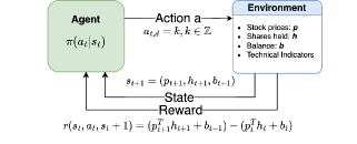
Figure 1: Stock trading as a reinforcement-learning problem.

We follow the practice of (Yang et al., 2020) by modeling the task of stock trading as a Markov Decision Process and subsequently train three deep reinforcement learning agents within it:

1. State $s=[p,h,b]$: A set including the prices of each stock $p\in\mathbb{R}^{D}$, the amount of each stock held in the portfolio $h\in\mathbb{Z}^{D}$, and the remaining balance in the account $b\in\mathbb{R}$, where $D$ denotes the total number of stocks considered.

2. Action $a$: a set of actions on all stocks $a\in\mathbb{R}^{D}$, which includes selling $k$ shares of stock $d$ ($a_{d}=-k$), buying $k$ shares of stock $d$ ($a_{d}=k$), and holding stock $d$ ($a_{d}=0$).

3. Reward function $r(s,a,s^{\prime})$: The change in portfolio value when action $a$ is taken at state $s$ to arrive at the new state $s^{\prime}$, where the total portfolio value is calculated as the sum of equities in all held stocks $p^{T}h$ and the remaining balance.

4. Policy $\pi(a|s)$: A probability distribution across $a$ at state $s$ that approximates an optimal trading strategy.

5. The action-value function $Q_{\pi}(s,a)$: The expected reward achieved if action $a$ is taken at state $s$ following the policy $\pi(s|a)$.

In this environment, an agent will aim to maximize their expected cumulative change in portfolio value following several market constraints and assumptions (liquidity, non-negative balance, and transaction costs).
We then simultaneously train three deep reinforcement learning agents in this environment, each corresponding to a different algorithm: Deep Deterministic Policy Gradient, Proximal Policy Optimization, and Advantage Actor Critic. To train and validate these algorithms, and to model the market according to the definitions above, we use the FinRL library – an open-source framework for integrating financial reinforcement learning strategies (Liu et al., 2020).

3.1.1 Deep Deterministic Policy Gradient

Deep Deterministic Policy Gradient (DDPG) is an off-policy deep reinforcement learning algorithm that concurrently learns both a Q-function and a policy gradient. It is a deep-learning extension of the Deterministic Policy Gradient algorithm (DPG) introduced by (Silver et al., 2014). Like its predecessor, DDPG utilizes actor and critic neural networks $\mu(s|\theta^{\mu})$ and $Q(s,a|\theta^{Q})$, where $\mu(s|\theta^{\mu})$ is an actor-network parametrized by $\theta^{\mu}$ that learns the optimal action to take given state $s$ and $Q(s,a|\theta^{Q})$ is a critic network parameterized by $\theta^{Q}$ that returns the estimated Q-value given action $a$ in state $s$.

Like other deep Q-learning algorithms, DDPG learns a Q-function $Q(s,a|\phi)$ by minimizing the mean-squared Bellman error:

$L(D)=\mathbb{E}_{t\in D}[(Q(s_{t},a_{t}|\phi)-y(t))^{2}]$, where

$y(t)=r(s_{t},a_{t})+\gamma(1-d_{t})max_{a^{\prime}}Q(s^{\prime}_{t},a^{\prime}|\phi)$

Here, $\phi$ describes the set of parameters in $Q$, and $t=(s_{t},a_{t},r_{t},s^{\prime}_{t},d_{t})$ describes an observation of a set of transitions in a replay buffer $D$, where $d_{t}$ indicates whether or not $s^{\prime}_{t}$ is a terminal state.

Rather than solely using the original networks themselves, DDPG creates copies of the actor and critic networks, $\mu^{\prime}(s|\theta^{\mu^{\prime}})$ and $Q^{\prime}(s,a|\theta^{Q^{\prime}})$, whose parameters are slowly updated by copying over a portion of the weights in their respective original networks (Lillicrap et al., 2019). These copies are then used to calculate the target value $y(t)$. Thus, Q-learning in DDPG is performed by minimizing:

$L(D)=E_{t\in D}[(Q(s_{t},a_{t}\phi)-y^{\prime}(t))^{2}]$, where

$y^{\prime}(t)=r(s_{t},a_{t})+\gamma(1-d_{t})max_{a^{\prime}}Q^{\prime}(s^{\prime},\mu^{\prime}(s^{\prime}|\theta^{\mu^{\prime}})|\theta^{Q^{\prime}})$

Since $\mu(s|\theta^{\mu})$ learns to output an action that maximizes $Q(s,a|\phi)$, traditional gradient ascent can be performed w.r.t. $\theta^{\mu}$ to solve

$max_{\theta^{\mu}}E_{s\in D}[Q(s,\mu(s|\theta^{\mu})|\phi)]$.

3.1.2 Proximal Policy Optimization

Proximal Policy Optimization (PPO) is a family of policy gradient methods that aims to optimize a surrogate objective function using stochastic gradient descent (Schulman et al., 2017a). The surrogate objective function ensures that gradient updates are not too large and that at each iteration the new learned policy is not significantly different from the previous one. The algorithm improves upon Trust Region Policy Optimization (Schulman et al., 2017b) by removing the need to incorporate Kullback-Leibler divergence into its deviation penalty and allowing updates that are compatible with stochastic gradient descent (Schulman et al., 2017a). Its objective function is defined as the maximization of:

$L^{PPO}=\mathbb{E}[min(R_{t}(\theta)A_{t},clip(R_{t}(\theta),1-\epsilon,1+\epsilon)A_{t})]$,

where $R_{t}(\theta)$ is the ratio of the probability distributions under the new and old policies:

$r_{t}(\theta)=\frac{\pi_{\theta}(a_{t}|s_{t})}{\pi_{\theta_{old}}(a_{t}|s_{t})}$,

$A_{t}$ is the estimated advantage at timestep $t$, and $\epsilon$ is a hyperparameter usually between 0.1 and 0.2 (Schulman et al., 2017a).

The integral observation of PPO is that it clips the relative amount of change in the parameters of a policy based on the estimated advantages. If, at a particular timestep, a policy’s actions are worse than its prior policy, then $A_{t}$ is negative, and the surrogate objective function $L^{PPO}$ can at most be $(1-\epsilon)A_{t}$. When actions under the new policy are deemed better than the old policy, then $A_{t}$ is positive, and the surrogate function ensures that $L^{PPO}$ can at most be $(1+\epsilon)A_{t}$, ensuring that policy changes at each iteration remain conservative (Schulman et al., 2017a). In practice, PPO is stable, fast, and simple to implement and tune.

3.1.3 Advantage Actor-Critic

Advantage actor-critic (A2C) is the synchronous variant of asynchronous advantage actor-critic (A3C) (Mnih et al., 2016). A2C is an actor-critic algorithm and utilizes an advantage function $A(a_{t},s_{t})=Q(a_{t},s_{t})-V(s_{t})$ to reduce the variance of policy gradients. The advantage function can be reduced through the Bellman recurrence to rely only on the approximation of $V$: $A(a_{t},s_{t})=r(s_{t},a_{t})+\gamma V(s^{\prime}_{t})-V(s_{t})$ (Mnih et al., 2016). In doing so, actions are evaluated not only on how good its raw value is but also how much better it is compared to the state baseline $V_{(}s_{t})$.

The gradient of the objective function of A2C is:

$\nabla L^{A2C}=E[\sum_{t=1}^{T}\nabla_{\theta}log_{\pi_{\theta}}(a_{t}|s_{t})A(s_{t},a_{t})]$

Similar to A3C, A2C disperses copies of the same agent to compute its gradients concerning different data samples (Mnih et al., 2016). Each agent interacts independently with the same environment, with the key difference between A3C and A2C being that the latter is a single-worker variant of the former: A2C runs interactions with a single copy of itself and waits for the computation of all gradients in a run before averaging and updating the global parameters. The practice of synchronizing gradients is cost-effective and efficient, and has empirically shown to produce results comparable to A3C.

3.2 Capturing Market Sentiment

Period	Sentiment
01/01/2010-03/04/2010	-4.33
03/05/2010-05/06/2010	0.37
05/07/2010-07/08/2010	17.56
07/09/2010-09/09/2010	-7.20
09/10/2010-11/12/2010	-26.20

Table 1: An example of captured sentiment for consecutive periods.

To capture market sentiment, we write a script that gathers daily headlines from leading financial news sources (Wall Street Journal, Bloomberg, etc.) and extracts their sentiments using the AFINN-en-165 sentiment lexicon. AFINN is a family of mappings of English terms and an integer rating valence between -5 and 5, where higher numbers indicate a more positive sentiment (Nielsen, 2011). In particular, AFINN-en-165 contains 3382 entries of words and phrases and is considered a general improvement over its predecessor, AFINN-111.

Our choice of designating news headlines as a source of sentiment stems from the general ideology that headlines must be simultaneously succinct, informative, and relevant for the sake of viewership and reputation. This makes them ideal candidates for extracting a general representation of a given subject. We focus our attention specifically on finance-related articles, since they respectively contain headlines whose sentiments coalesce into a near-accurate portrayal of the contemporary market.

The total sentiment of a headline can thus be expressed as the average of the sentiments of its comprised words, and the sentiment for a given period is the total sum of the sentiments of headlines published during that period:

$Sentiment(p)=\sum_{i\in p}\frac{1}{|T_{i}|}\sum_{k=0}^{|T_{i}|}score(T_{i}[k])$,

where $T_{i}[k]$ describes the $k$th word of the $i$th headline, $|T_{i}|$ describes the length (in words) of headline $i$, and $p$ denotes the length of the period.

In contrast with other sentiment-based prediction processes, our method is simple, efficient, and easy to implement. By taking advantage of pre-existing lexicons rather than learning scores from scratch, we are able to instantaneously retrieve and calculate the average news sentiment over a period of time.

3.3 Dynamic Learning Adaptation

3.3.1 Choosing an Agent

We modify the method of (Yang et al., 2020) and determine the best-performing algorithm to be that which results in the highest relative Sharpe-Sortino ratio after validation.

The Sharpe ratio measures a portfolio’s return compared to its risk, or standard deviation. It is defined as:

$Sharpe=\frac{R_{p}-R_{f}}{\sigma_{p}}$

Where $R_{p}$ is the portfolio return, $R_{f}$ is the risk-free rate, and $\sigma_{p}$ is the standard deviation of the portfolio. The Sortino ratio is similar to the Sharpe ratio but only penalizes downside volatility. It is defined as:

$Sortino=\frac{R_{p}-R_{f}}{\sigma_{d}}$

Where $\sigma_{d}$ is the standard deviation of the portfolio’s negative returns or downside. Thus, our final scoring metric is:

$\chi_{i}=\alpha*Sharpe+(1-\alpha)*Sortino$

Where $\alpha$ is a hyperparameter selected before training, and $\chi_{i}$ denotes the post-validation performance of agent $i$.

3.3.2 Switching Agents

Lastly, our algorithm will only switch trading agents when it has detected a change in period-to-period sentiment above a certain predetermined threshold $\beta$. The intuition behind this methodology is that because agents trained on different reinforcement learning frameworks perform differently across environments, an optimal trading strategy will derive from the practice of detecting events monumental enough to affect markets and cause a dramatic shift in public sentiment, and subsequently re-selecting the best-performing agent based on the most recent data.

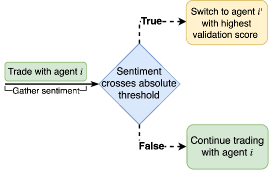
Figure 2: Overview of proposed algorithm.

Figure 2. describes the general process in which we select agents. The first selected agent will be that which results in the highest initial validation score, $Agent=argmax_{i\in A}(\chi_{i})$. Following this, we validate agents in parallel and repeatedly gather daily news sentiments from a pre-selected database of financial sources. If the sentiment score for a given period exceeds a predetermined absolute threshold, then we switch to using the agent which currently holds the highest validation score for the given period. If the sentiment score does not exceed the threshold, then we deduce that market conditions have likely not drastically changed, and simply continue using the agent currently in selection since it has been shown to perform well in this environment.

4 Evaluating Our Agent

We evaluate our strategy by training and testing on historical stock data - a practice commonly known as backtesting. For comparison, we also evaluate the performance of the standard ensemble algorithm, a single DDPG agent, and the Dow Jones Industrial Average (DJIA) (Yang et al., 2020). All deep-learning based algorithms (ours, ensemble, DDPG) are trained and tested on the same time period and data.

Specifically, our agents are trained for seven years on stock data (1/1/2010 through 12/31/2016) and then evaluated over a two-year period on out-of-sample data (04/04/2017 through 04/01/2019). For sentiment analysis, we used business articles from the Wall Street Journal Archive, with 15 articles gathered daily to generate an approximation of daily financial sentiment. For hyperparameters, an $\alpha$ of 0.25 was selected for measuring validation performance ($25\%$ Sharpe, $75\%$ Sortino) and a $\beta$ of 15 was determined as a sentiment score threshold for switching agents. These values were empirically observed to result in the most optimal trading strategy.

Table 1. shows the results of each strategy’s performance during the evaluation period, and their performance relative to that of others is visualized in Figure 1. Our Sentiment-Ensemble strategy significantly outperforms both the Dow Jones and the ensemble strategy, resulting in a cumulative return of over 40% over the two-year period and an annualized return of 18.36%. Additionally, we find that our method results in the highest Sharpe and Sortino Ratio and the lowest maximum drawdown by a notable margin, suggesting that it learns to better manage the risk-over-return trade-off. We also note that an individual deep reinforcement strategy (DDPG) outperforms the traditional ensemble strategy on its own, but falls behind our sentiment-paired approach. We hypothesize that this indicates that traditional $n$-period agent switching is not an effective way to allocate agents in an ensemble strategy, and that a more optimal use of the method involves the introduction of utilizing market sentiment.

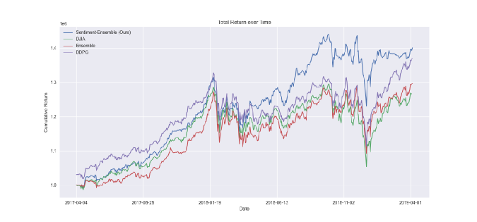
Figure 3: Performance of our algorithm (blue) against the ensemble strategy (red), a DDPG agent (purple) and the Dow Jones Industrial Average (green).

	Sentiment-Ensemble (Ours)	Ensemble	DDPG	DJIA
Cumulative Return	40.10%	29.65%	33.72%	26.72%
Annual Return	18.36%	13.86%	12.86%	12.60%
Maximum Drawdown	-14.57%	-15.43%	-16.12%	-18.77%
Annual Volatility	13.50%	14.49%	13.04%	14.18%
Sharpe Ratio	1.32	0.97	0.99	0.91
Sortino Ratio	1.87	1.34	1.34	1.25

Table 2: Performance metrics for Sentiment-Ensemble (our method), the conventional ensemble strategy (Yang et al., 2020), a DDPG agent (Liu et al., 2022), and the Dow-Jones as a benchmark. All deep-learned agents were trained on stock data from 1/1/2010 to 12/31/2016 and then evaluated from 04/04/2017 to 04/01/2019.

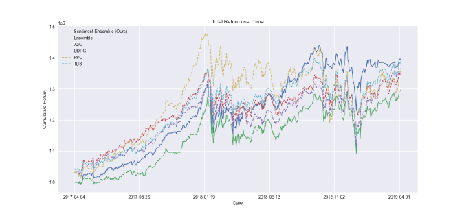
Figure 4: Return over time of Sentiment-Ensemble (blue) and ensemble (green) against A2C (dashed-red), DDPG (dashed-purple), PPO (dashed-yellow), and TD3 (dashed-blue).

	S-E	Ensemble	DDPG	A2C	PPO	TD3
Cumulative Return	40.10%	29.65%	33.72%	32.40%	27.49%	35.30%
Annual Return	18.36%	13.86%	12.86%	12.40%	10.65%	13.42%
Maximum Drawdown	-14.57%	-15.43%	-16.12%	-15.05%	-22.35%	-17.84%
Annual Volatility	13.50%	14.49%	13.04%	13.76%	17.39%	13.83%
Sharpe Ratio	1.32	0.97	0.99	0.92	0.67	0.98
Sortino Ratio	1.87	1.34	1.34	1.30	0.93	1.38

Table 3: Performance metrics for Sentiment-Ensemble and ensemble against DDPG, A2C, PPO, and TD3. All deep-learned agents were trained on the same stock data from 1/1/2010 to 12/31/2016 and then evaluated from 04/04/2017 to 04/01/2019

.

To confirm our hypothesis, we compare the performance of Sentiment-Ensemble (our method) and ensemble against the individual algorithms that both strategies comprise: DDPG, PPO, and A2C (Table 3). In addition, we evaluate an algorithm separate from the ones learned in ensemble, Twin Delayed DDPG (TD3) (Fujimoto et al., 2018). We find that in all cases, ensemble performs worse than its single-agent components, as well as unrelated single-agent algorithms. However, when paired with dynamic sentiment analysis, our method manages to outperform every other strategy, despite leveraging the exact same agents as ensemble. By examining Figure 4, we notice that Sentiment-Ensemble appears to better merge the behavior of its component algorithms – the goal of ensemble-learning – before subsequently outperforming them.

5 Conclusion

To the best of our knowledge, we present the first successful integration of sentiment analysis into deep-reinforcement learning ensemble strategies designed for live stock trading. To achieve this, we introduce a simple-yet-effective methodology of extracting market sentiment, and incorporate this into a strategy that combines qualitative market properties with agents trained on quantitative data. Our method results in a strategy that outperforms the current state-of-the-art ensemble approach, showing that the conventional method of switching agents every $n$ months, where $n$ is fixed, is not as effective as dynamically switching agents based on environmental changes. In addition, our algorithm for extracting market sentiment is simple and efficient, and we encourage the transition of our method into real-time trading on live data, as it should be a relatively simple to implement.

Some possible future directions of interest involve exploring more sophisticated sentiment-detection strategies that employ a similar level of efficiency, such as performing inference with external large language models (LLMs) that may potentially capture market dynamics better. Additionally, the threshold for sentiment ($\beta$) could be more effectively learned, rather than set, by an external “management” network, which learns to manage and disperse its respective agents.

References

- Nathan et al. (2023) Allison Nathan, Jenny Grimberg, and Ashley Rhodes. Top of mind - u.s. outperformance: At a turning point? Goldman Sachs Global Macro Research, 2023.
- Yang et al. (2020) Hongyang Yang, Xiao-Yang Liu, Shan Zhong, and Anwar Walid. Deep reinforcement learning for automated stock trading: An ensemble strategy. Social Science Research Network, 2020.
- Liu et al. (2022) Xiao-Yang Liu, Zhuoran Xiong, Shan Zhong, Hongyang Yang, and Anwar Walid. Practical deep reinforcement learning approach for stock trading, 2022.
- Li et al. (2022) Fangyi Li, Zhixing Wang, and Peng Zhou. Ensemble investment strategies based on reinforcement learning. Handawi, 2022.
- Yu et al. (2023) Xiaoming Yu, Wenjun Wu, Xingchuang Liao, and Yong Han. Dynamic stock-decision ensemble strategy based on deep reinforcement learning. Applied Intelligence, 2023.
- Mnih et al. (2013) Volodymyr Mnih, Koray Kavukcuoglu, David Silver, Alex Graves, Ioannis Antonoglou, Daan Wierstra, and Martin Riedmiller. Playing atari with deep reinforcement learning, 2013.
- Jiang et al. (2017) Zhengyao Jiang, Dixing Xu, and Jinjun Liang. A deep reinforcement learning framework for the financial portfolio management problem, 2017.
- Liu et al. (2020) Xiao-Yang Liu, Hongyang Yang, Qian Chen, Runjia Zhang, Liuqing Yang, Bowen Xiao, and Christina Dan Wang. FinRL: A deep reinforcement learning library for automated stock trading in quantitative finance. Deep RL Workshop, NeurIPS 2020, 2020.
- Bai et al. (2023) Zeng-Liang Bai, Ya-Ning Zhao, Zhi-Gang Zhou, Wen-Qin Li, Yang-Yang Gao, Ying Tang, Long-Zheng Dai, and Yi-You Dong. Mercury: A deep reinforcement learning-based investment portfolio strategy for risk-return balance. IEEE Access, 11:78353–78362, 2023. doi: 10.1109/ACCESS.2023.3298562.
- Mittal and Goel (2012) Anshul Mittal and Arpit Goel. Stock prediction using twitter sentiment analysis. 2012.
- Kalyani et al. (2016) Joshi Kalyani, Prof. H. N. Bharathi, and Prof. Rao Jyothi. Stock trend prediction using news sentiment analysis, 2016.
- Xiao and Ihnaini (2023) Qianyi Xiao and Baha Ihnaini. Stock trend prediction user sentiment analysis. PeerJ Computer Science, 2023.
- Silver et al. (2014) David Silver, Guy Lever, Nicolas Heess, Thomas Degris, Daan Wierstra, and Martin Riedmiller. Deterministic policy gradient algorithms. In International Conference on Machine Learning, 2014.
- Lillicrap et al. (2019) Timothy P. Lillicrap, Jonathan J. Hunt, Alexander Pritzel, Nicolas Heess, Tom Erez, Yuval Tassa, David Silver, and Daan Wierstra. Continuous control with deep reinforcement learning, 2019.
- Schulman et al. (2017a) John Schulman, Filip Wolski, Prafulla Dhariwal, Alec Radford, and Oleg Klimov. Proximal policy optimization algorithms, 2017a.
- Schulman et al. (2017b) John Schulman, Sergey Levine, Philipp Moritz, Michael I. Jordan, and Pieter Abbeel. Trust region policy optimization, 2017b.
- Mnih et al. (2016) Volodymyr Mnih, Adrià Puigdomènech Badia, Mehdi Mirza, Alex Graves, Timothy P. Lillicrap, Tim Harley, David Silver, and Koray Kavukcuoglu. Asynchronous methods for deep reinforcement learning, 2016.
- Nielsen (2011) Finn Årup Nielsen. A new ANEW: evaluation of a word list for sentiment analysis in microblogs. In Matthew Rowe, Milan Stankovic, Aba-Sah Dadzie, and Mariann Hardey, editors, Proceedings of the ESWC2011 Workshop on ’Making Sense of Microposts’: Big things come in small packages, volume 718 of CEUR Workshop Proceedings, pages 93–98, May 2011. URL http://ceur-ws.org/Vol-718/paper_16.pdf.
- Fujimoto et al. (2018) Scott Fujimoto, Herke van Hoof, and David Meger. Addressing function approximation error in actor-critic methods, 2018.