Computing scattering resonances of rough obstacles

Abstract.

This paper is concerned with the numerical computation of scattering resonances of the Laplacian for Dirichlet obstacles with rough boundary. We prove that under mild geometric assumptions on the obstacle there exists an algorithm whose output is guaranteed to converge to the set of resonances of the problem. The result is formulated using the framework of Solvability Complexity Indices. The proof is constructive and provides an efficient numerical method. The algorithm is based on a combination of a Glazman decomposition, a polygonal approximation of the obstacle and a finite element method. Our result applies in particular to obstacles with fractal boundary, such as the Koch Snowflake and certain filled Julia sets. Finally, we provide numerical experiments in MATLAB for a range of interesting obstacle domains.

1. Introduction

Scattering resonances of the Laplace operator play a fundamental role in quantum mechanics and acoustics, encoding the behaviour of the wave and free Schrödinger equations [11]. The non-self-adjoint nature of the problem poses challenges for the construction of stable and convergent numerical algorithms. Current methods include complex scaling (as well as the closely related method of perfectly matched layers), boundary integral methods and various modifications of the finite element method. The study of the foundations of computation for scattering resonances was recently initiated in [4, 5] within the framework of Solvability Complexity Indices [15, 3, 2, 9, 8].

Meanwhile, in the context of wave propagation and spectral theory, fractal boundaries are responsible for a variety of striking phenomena. Notably, they are particularly efficient for wave absorption [14] and give rise to exotic eigenvalue asymptotics (see [13, 17, 18, 22, 19] for instance and references therein). In our previous article [26], we investigated the computability of eigenvalues of the Dirichlet Laplacian on bounded domains. Our results revealed that eigenvalues are computable in one limit for a wide class of domains with rough boundaries, however, for large enough classes of domains, with sufficiently irregular boundaries, the problem becomes non-computable.

In this article, we study the numerical computation of scattering resonances for the Laplacian on exterior domains in the plane, that is domains of the form $U^{c}=\mathbb{R}^{2}\backslash U$ for closed and bounded $U\subset\mathbb{R}^{2}$, endowed with Dirichlet boundary conditions. This setting is often referred to as obstacle scattering and $U$ as the obstacle. The novelty of our article is that we only impose very mild geometric conditions on the boundary of the domain, allowing for a wide variety of fractal boundaries. Our primary contributions are as follows:

1. We introduce a fast and simple numerical algorithm for scattering resonances with rough boundaries.

2. We prove convergence of this algorithm (see Theorem 2.13), from which we deduce an upper bound for the computational complexity of the problem (see Theorem 2.3). Our sole geometric assumption on the domain that its boundary is a union of a finite number of closed Jordan curves with zero area.

3. We perform numerical investigations for scattering resonances for Koch snowflake and filled Julia set obstacles. See Section 6.

Our algorithm is a modification of one introduced by Levitin and Marletta [20] (see Remark 2.8). It is based on domain decomposition, Neumann-to-Dirichlet (NtD) operators, spectral expansions and the finite element method (FEM). This gives rise to several sources of approximation error, including:

• Geometric error due to the approximation of rough boundaries by polygonal ones.

• FEM discretisation error.

• Truncation error due to approximation of NtD operators by finite matrices.

These sources of error are estimated and linked in order to ensure convergence in one limit (see Assumption 2.12). The proof of our main convergence theorem is based on utilising the notion of Mosco convergence in conjunction with Gohberg-Sigal theory.

Our SCI result (Theorem 2.3) generalises the aforementioned work [4]. While the result in [4] proves existence of a convergent algorithm for scattering resonances of obstacles with $C^{2}$ boundary, we deal with a vastly wider class of obstacles. Other closely related works include similar algorithms in other settings [21, 25], the boundary element method for fractal screens [7] and shape optimisation for rough domains [16].

2. Overview of results

In this section, we provide the necessary background for scattering resonances, state our main results and provide details of our numerical method.

2.1. Scattering resonances

Let $U\subset\mathbb{R}^{2}$ denote a closed, bounded set and consider the Laplacian $H$ on the the exterior domain $U^{c}=\mathbb{R}^{2}\backslash U$ endowed with homogeneous Dirichlet boundary conditions on $\partial U$,

$$H=-\Delta,\qquad D(H)=\{u\in H^{1}_{0}(U^{c}):\Delta u\in L^{2}(U^{c})\}$$

where $D(H)$ denotes the domain of the operator $H$ and we employ standard notation for Sobolev spaces ($H^{1}$, $H^{1}_{0}$ etc.). Let $X>0$ be large enough so that $U\subset B_{X-1}(0)$ (throughout, $B_{r}(0)$ shall denotes a ball in $\mathbb{R}^{2}$ of radius $r>0$ centred at the origin). For simplicity, we restrict our attention to scattering resonances in $\mathbb{C}_{-}$.

Let $\chi$ be a smooth, compactly supported function such that $\chi\equiv 1$ on $B_{X}(0)$. Then, by [11, Theorem 4.4], the analytic operator-valued function

(2.1) $$\chi(H-k^{2})^{-1}\chi:L^{2}(\mathbb{R}^{2})\to L^{2}(\mathbb{R}^{2}),\qquad k\in\mathbb{C}_{+},$$

admits a meromorphic continuation to $k\in\mathbb{C}\backslash(-\infty,0]$.

Definition 2.1.

The scattering resonances of $H$ are defined as the poles of $\chi(H-k^{2})^{-1}\chi$ in $\mathbb{C}_{-}$.

2.2. Main computational complexity result

Consider a computational problem described by the following elements.

1. Let $\mathcal{S}$ denote the set of closed, bounded sets $U\subset\mathbb{R}^{2}$ (representing obstacles) such that the following holds.

   • $U$ has a finite number of connected components and is the closure of an open set.

   • Each connected component of $\partial U$ is path-connected and has zero Lebesgue measure (i.e. zero area).

   $\mathcal{S}$ is referred to as the primary set and represents the class of admissible obstacles. Examples of elements $U\in\mathcal{S}$ include the Koch snowflake and certain filled Julia sets (see Section 6.3 and 6.2 respectively).

2. Define a metric space $\mathcal{M}:=(\mathrm{cl}(\mathbb{C}_{-}),\mathrm{d}_{\mathrm{AW}})$, where $\mathrm{cl}(\mathbb{C}_{-})$ denotes the set of closed, non-empty subsets of $\mathbb{C}_{-}$ and $\mathrm{d}_{\mathrm{AW}}$ denotes the Attouch-Wets distance,

   (2.2) $$d_{\text{AW}}(A,B)=\sum_{k=1}^{\infty}2^{-k}\min\left\{1\,,\,\sup_{|x|<k}\left|\operatorname{dist}(x,A)-\operatorname{dist}(x,B)\right|\right\}.$$

   Note that if $A,B\subset\mathbb{R}^{d}$ are bounded, then $d_{\text{AW}}$ is equivalent to the Hausdorff distance.

3. Let $\mathrm{Res}:\mathcal{S}\to\mathcal{M}$ denote the map which, for any obstacle $U\in\mathcal{S}$, gives the corresponding set of scattering resonances in $\mathbb{C}_{-}$. This is referred to as the problem function.

4. Consider a set of real-valued maps defined by

   (2.3) $$\Lambda=\{U\mapsto\mathbbm{1}_{U}(x):x\in\mathbb{R}^{2}\},$$

   where $\mathbbm{1}_{U}$ denotes the characteristic function of $U$. This is referred to as the evaluation set and represents the information available to an algorithm.

Together, the quadruple $\{\mathrm{Res},\mathcal{S},\mathcal{M},\Lambda\}$ formally constitutes a computational problem in the language of Solvability Complexity Indices, which may be summarised as:

$$\textrm{Compute the scattering resonances for obstacles in }\mathcal{S}\textrm{, given access point values of }\mathbbm{1}_{U}\textrm{.}$$

Intuitively, an arithmetic algorithm for this computational problem is a map $\Gamma:\mathcal{S}\to\mathcal{M}$ which produces its output by performing a finite number of arithmetic operations on $\mathbbm{1}_{U}(x_{1})$,…,$\mathbbm{1}_{U}(x_{N})$ for some sample points $x_{1},...,x_{N}\in\mathbb{R}^{d}$, which may depend on $U$. This notion is formalised as follows.

Definition 2.2 (Arithmetic algorithm).

Let $\{\Xi,\mathcal{S},\mathcal{M},\Lambda\}$ be a computational problem. An arithmetic algorithm is a mapping $\Gamma:\mathcal{S}\to\mathcal{M}$ such that for each $U\in\mathcal{S}$

1. there exists a finite (non-empty) subset $\Lambda_{\Gamma}(U)\subset\Lambda$,

2. the action of $\Gamma$ on $U$ depends only on $\{f(U)\}_{f\in\Lambda_{\Gamma}(U)}$ and the output is obtained by a finite number of arithmetic operations,

3. for every $U_{2}\in\mathcal{S}$ with $f(U_{2})=f(U_{1})$ for all $f\in\Lambda_{\Gamma}(U_{1})$ one has $\Lambda_{\Gamma}(U_{1})=\Lambda_{\Gamma}(U_{2})$.

Our first result reads as follows.

Theorem 2.3.

There exists a sequence of arithmetic algorithms $\Gamma_{n}:\mathcal{S}\to\mathcal{M}$, $n\in\mathbb{N}$, for the computational problem $\{\mathrm{Res},\mathcal{S},\mathcal{M},\Lambda\}$ such that

(2.4) $$\forall\,U\in\mathcal{S}:\qquad\mathrm{d}_{\mathrm{AW}}(\Gamma_{n}(U),\mathrm{Res}(U))\to 0\qquad\text{as}\qquad n\to\infty.$$

In the language of SCI, Theorem 2.3 may be written

(2.5) $$\{\mathrm{Res},\mathcal{S},\mathcal{M},\Lambda\}\in\Delta_{2}^{A},$$

where $\Delta_{2}^{A}$ refers to the fact that the result states convergence in one limit with arithmetic algorithms.

2.3. Domain decomposition definition

Next, we define scattering resonances via an alternative domain decomposition approach, from which our numerical method will naturally follow. Decompose $U^{c}$ into an inner domain, an outer domain and an interface as (see Figure 1)

(2.6) $$\Omega:=B_{X}(0)\backslash U,\qquad\Omega_{\mathrm{out}}:=\mathbb{R}^{2}\backslash\overline{B_{X}(0)}\qquad\text{and}\qquad\Gamma:=\partial B_{X}(0).$$

Let $\{e_{\alpha}\}_{\alpha\in\mathbb{Z}}$ denote an orthonormal basis for $L^{2}(\Gamma)$ defined by

$$e_{\alpha}(\theta):=\frac{1}{\sqrt{2\pi X}}e^{i\alpha\theta},\qquad\alpha\in\mathbb{Z}.$$

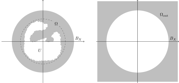
Figure 1. Sketch of the definitions of $\Omega$ and $\Omega_{\text{out}}$. The dashed line in the left figure indicates $B_{X-1}(0)$.

Consider the boundary value problem

(2.7) $$\begin{cases}-\Delta u=k^{2}u\quad\text{on}\quad U^{c}\\ u|_{\partial U}=0\end{cases},\qquad k\in\mathbb{C},$$

so that, in particular, $k^{2}$ is an eigenvalue of $H$ if and only if there exists a non-trivial solution $u$ of (2.7) in $L^{2}(U^{c})$. Let $H^{(1)}_{n}$ and $H^{(2)}_{n}$ denote the Hankel functions of the first and second kind (of order $n$) respectively. For $k\neq 0$, the general form for solutions of $-\Delta u=k^{2}u$ on the outer domain $\Omega_{\mathrm{out}}$ is

(2.8) $$u(x;k)=\sum_{\alpha\in\mathbb{Z}}\left(q_{\alpha}H^{(1)}_{|\alpha|}(k|x|)e_{\alpha}(\theta(x))+\tilde{q}_{\alpha}H^{(2)}_{|\alpha|}(k|x|)e_{\alpha}(\theta(x))\right),$$

where $q_{\alpha}$ and $\tilde{q}_{\alpha}$ are sequences of complex numbers such that $(q_{\alpha}H^{(1)}_{|\alpha|}(k|x|))_{\alpha\in\mathbb{Z}},(\tilde{q}_{\alpha}H^{(2)}_{|\alpha|}(k|x|))_{\alpha\in\mathbb{Z}}\in\ell^{1}(\mathbb{Z})$ and $\theta(x)$ is the angular part of $x$. We select only the “first kind solutions” (i.e. the ones with $\tilde{q}_{\alpha}=0$); these are precisely the set of solutions that are in $L^{2}(\Omega_{\mathrm{out}})$ when $k\in\mathbb{C}_{+}$ (throughout, $\mathbb{C}_{\pm}=\{z\in\mathbb{C}:\pm\operatorname{Im}\,z>0\}$). Furthermore, it is convenient to re-parametrise $q_{\alpha}$, in order to cancel out the rapid growth of the Hankel functions of first kind for large order,

(2.9) $$H^{(1)}_{\nu}(kX)\sim A_{\nu}:=-i\sqrt{\frac{2}{\pi\nu}}\left(\frac{ekX}{2\nu}\right)^{-\nu}\qquad\text{as}\qquad\nu\to\infty.$$

We therefore seek solutions of (2.7) which take the following form on $\Omega_{\mathrm{out}}$,

(2.10) $$u_{q}(x;k):=\sum_{\alpha\in\mathbb{Z}}q_{\alpha}\frac{1}{A_{|\alpha|}}H^{(1)}_{|\alpha|}(k|x|)e_{\alpha}(\theta(x)),\qquad q\in\ell^{1}(\mathbb{Z}),$$

where the summability condition on $q$ ensures convergence of the sum. The solutions $u_{q}(x;k)$, $x\in\Omega_{\mathrm{out}}$, are defined and form analytic functions for $k\in\mathbb{C}\backslash(-\infty,0]$. Furthermore, $u_{q}(\cdot;k)$ are square-integrable if and only if $k\in\mathbb{C}_{+}$ (in fact, $u_{q}(\cdot;k)$ is exponentially decaying as $|x|\to\infty$ if $k\in\mathbb{C}_{+}$ and exponentially growing if $k\in\mathbb{C}_{-}$).

Definition 2.4.

We call a number $k\in\mathbb{C}\backslash(-\infty,0]$ a scattering resonance of $H$ if there exists a non-zero solution of boundary value problem (2.7) taking the form $u_{q}(\cdot;k)$ in $\Omega_{\mathrm{out}}$.

Remark 2.5.

In particular, the (square roots of) eigenvalues of $H$ correspond to scattering resonances in the upper half plane as per definition 2.4 (note that $H$ happens not to have any eigenvalues in our setting).

Remark 2.6.

Definition 2.4 for scattering resonances can be seen to be equivalent to the definition via meromorphic continuation of the resolvent (Definition 2.1). Indeed, scattering resonances, as per the definition via meromorphic continuation, are characterised as the points for which there exists a corresponding resonant state [11, Theorem 4.7, Definition 4.8]. In turn, resonant states can be shown [11, Definition 4.9] to be characterised as the functions $u\in L^{2}_{\mathrm{loc}}(U^{c})$ with $\chi u\in D(H)$ such that

(2.11) $$(-\Delta-k^{2})u=0\qquad\text{on}\qquad U^{c},$$

and there exists compactly supported $g\in L^{2}(\mathbb{R}^{2})$ such that

(2.12) $$u|_{B_{X}(0)^{c}}=R_{0}(k)g|_{B_{X}(0)^{c}},$$

where $R_{0}(k)=(-\Delta-k^{2})^{-1}$ denotes the analytic continuation of the free resolvent on $L^{2}(\mathbb{R}^{2})$. It can then be readily seen that $u$ is a resonant state corresponding to $k\in\mathbb{C}_{-}\backslash(-\infty,0]$ if and only if it solves (2.7) and takes the form $u_{q}(\cdot;k)$ in $\Omega_{\mathrm{out}}$.

2.4. Operator theoretic characterisation

Next, we express scattering resonances in the lower half plane in terms of a natural interface condition that will form the basis of our numerical method below. Introduce the diagonal operator on $L^{2}(\Gamma)$,

(2.13) $$\mathcal{N}:=\operatorname{diag}(\max\{|\alpha|,1\},\alpha\in\mathbb{Z}).$$

We define fractional Sobolev spaces on $\Gamma$ as

(2.14) $$H^{s}(\Gamma):=\mathcal{N}^{-s}L^{2}(\Gamma),\qquad s\in\mathbb{R}.$$

The inner NtD operator $M_{\mathrm{in}}(k)$ is defined as

$$M_{\mathrm{in}}(k)g:=\gamma_{\Gamma}u_{\mathrm{in}}\qquad k\in\mathbb{C}_{+},\quad g\in H^{-\frac{1}{2}}(\Gamma),$$

where the function $u_{\mathrm{in}}\in H^{1}_{\mathrm{ND}}(\Omega):=\{u|_{\Omega}:u\in H^{1}_{0}(U^{c})\}$ is defined as the weak solution to the boundary value problem

(2.15) $$\begin{cases}-\Delta u_{\mathrm{in}}=k^{2}u_{\mathrm{in}}\quad\text{on}\quad\Omega\\ u_{\mathrm{in}}|_{\partial U}=0,\quad\partial_{\nu}|_{\Gamma}u_{\mathrm{in}}=g\end{cases}.$$

Here, $\gamma_{\Gamma}$ denotes the trace operator for $\Gamma$. As is well known, $M_{\mathrm{in}}$ forms an analytic family of bounded operators from $H^{-\frac{1}{2}}(\Gamma)$ to $H^{\frac{1}{2}}(\Gamma)$ on $\mathbb{C}_{+}$ and admits meromorphic continuation to $\mathbb{C}$ which, in particular, is analytic in $\mathbb{C}_{-}$.

Furthermore, for $k\in\mathbb{C}\backslash(-\infty,0]$, introduce the diagonal operators

(2.16) $$N_{1}(k):=\operatorname{diag}\left(\frac{1}{A_{|\alpha|}}H^{(1)}_{|\alpha|}(kX),\alpha\in\mathbb{Z}\right)\quad\text{and}\quad N_{2}(k):=\operatorname{diag}\left(\frac{1}{A_{|\alpha|}}(H_{|\alpha|}^{(1)})^{\prime}(kX),\alpha\in\mathbb{Z}\right).$$

$N_{1}(k)$ is a bounded operator from $H^{\frac{1}{2}}(\Gamma)$ to $H^{\frac{1}{2}}(\Gamma)$ whereas, by the large order asymptotics for derivatives of Hankel functions of the first kind,

(2.17) $$(H_{\nu}^{(1)})^{\prime}(kX)\sim-\frac{\nu}{kX}A_{\nu}\qquad\text{as}\qquad\nu\to\infty,$$

$N_{2}(k)$ is a bounded operator from $H^{\frac{1}{2}}(\Gamma)$ to $H^{-\frac{1}{2}}(\Gamma)$. By definition, we have

(2.18) $$N_{1}(k)q=\gamma_{\Gamma}u_{q}(\cdot;k)\qquad\text{and}\qquad N_{2}(k)q=\partial_{\nu}|_{\Gamma}u_{q}(\cdot;k)$$

A function $u$ solves the BVP (2.7) if and only if

(2.19) $$\begin{cases}-\Delta u=k^{2}u\quad\text{on}\quad\Omega_{\mathrm{out}}\\ u|_{\Gamma}=-M_{\mathrm{in}}(k)g,\quad\partial_{\nu}|_{\Gamma}u=g\end{cases}$$

for some $g\in H^{-1/2}(\Gamma)$ hence, in particular, satisfies $u|_{\Gamma}=-M_{\mathrm{in}}(k)\partial_{\nu}|_{\Gamma}u$. Therefore, a number $k\in\mathbb{C}_{-}$ is a scattering resonance of $H$ (as per Definition 2.4) if and only if

(2.20) $$\exists\,q\in H^{\frac{1}{2}}(\Gamma):\qquad(N_{1}(k)+M_{\mathrm{in}}(k)N_{2}(k))q=0.$$

We may convert the operator in (2.20) to an equivalent operator on $L^{2}(\Gamma)$ by bordering with appropriate powers of $\mathcal{N}$,

(2.21) $$T(k):=\frac{1}{2}\mathcal{N}^{\frac{1}{2}}(N_{1}(k)+M_{\mathrm{in}}(k)N_{2}(k))\mathcal{N}^{-\frac{1}{2}},\qquad k\in\mathbb{C}_{-}.$$

Note that in Appendix A, we prove that $T(k)$ is Fredholm of index zero. We arrive at our operator theoretic characterisation for scattering resonances of $H$.

Lemma 2.7.

A number $k\in\mathbb{C}_{-}$ is a scattering resonance of $H$ if $\ker\,T(k)\neq\{0\}$.

2.5. Algorithm for computing scattering resonances

We shall numerically compute scattering resonances by approximating the operator $T(k)$ by a matrix $T_{n}(k)$ with computable matrix elements. The index $n$ controls the accuracy of the computation and we anticipate convergence as $n\to\infty$. There are several simultaneous processes that take place, each giving rise to sources of error.

• Finite truncation of the infinite matrix $T(k)$ (expressed in the basis $\{e_{\alpha}\}$).

• Polygonal approximation of the obstacle $U$.

• Finite element approximation (FEM) of the inner NtD map $M_{\mathrm{in}}(k)$.

• The FEM approximation of $M_{\mathrm{in}}(k)$ is itself efficiently approximated by a truncated eigenfunction expansion and a trick known as Aitken’s acceleration.

Linking these different approximations in a way that ensures convergence is non-trivial and is clarified by the assumptions of our main result Theorem 2.13 below as well as numerical experiments in Section 6.

Matrix elements and truncation

Fix a sequence of parameters $N_{n}\in\mathbb{N}$, $n\in\mathbb{N}$ which control the number basis elements taken in matrix truncation. Consider the orthogonal projection

(2.22) $$P_{n}:L^{2}(\Gamma)\to\mathrm{span}_{\mathbb{C}}\{e_{-N_{n}},...,e_{N_{n}}\}.$$

The inner NtD operator may be expressed as infinite matrices with matrix elements

(2.23) $$a_{\alpha\beta}(k):=(M_{\mathrm{in}}(k)e_{\alpha},e_{\beta})_{L^{2}(\Gamma)},\qquad k\in\mathbb{C}_{-},\quad\alpha,\beta\in\mathbb{Z}.$$

Then, $P_{n}T(k)P_{n}$ is a $(2N_{n}+1)\times(2N_{n}+1)$ matrix with matrix elements

(2.24) $$T_{\alpha\beta}(k)=\frac{\delta_{\alpha\beta}}{2A_{|\alpha|}}H^{(1)}_{|\alpha|}(kX)+a_{\alpha\beta}(k)\frac{\max\{|\alpha|,1\}^{-\frac{1}{2}}\max\{|\beta|,1\}^{\frac{1}{2}}}{2A_{|\alpha|}}\left(H^{(1)}_{|\alpha|-1}(kX)-\frac{|\alpha|}{kX}H^{(1)}_{|\alpha|}(kX)\right)$$

where $\delta_{\alpha\beta}$ denotes the Kronecker delta symbol and we used the formula

(2.25) $$(H^{(1)}_{\nu})^{\prime}(z)=H^{(1)}_{\nu-1}(z)-\frac{\nu}{z}H^{(1)}_{\nu}(z).$$

The Hankel functions in $T_{\alpha\beta}(k)$ may be efficiently numerically computed using known methods, however, the computation of $a_{\alpha\beta}(k)$ requires more work.

Geometric approximation

Let $U_{n}\subset B_{X-1}(0)$, $n\in\mathbb{N},$ denote a sequence of closed, bounded sets with polygonal boundaries approximating the obstacle $U$. Let $B^{n}_{X}\subset B_{X}(0)$ be a sequence of convex, polygonal domains approximating $B_{X}(0)$ in the sense that

(2.26) $$B_{X}(0)=\bigcup_{n=1}^{\infty}B_{X}^{n},$$

such that the corners of $B^{n}_{X}$ lie on $\Gamma$. Polygonal approximations for the inner domain and interface may then be defined as

(2.27) $$\Omega_{n}:=B_{X}^{n}\backslash U_{n}\qquad\text{and}\qquad\Gamma_{n}:=\partial B_{X}^{n},\qquad n\in\mathbb{N}.$$

FEM approximation at a fixed point

For each $n\in\mathbb{N}$, let $\mathcal{T}_{n}$ be a triangulation of $\Omega_{n}$ and consider the P1 finite element spaces

(2.28) $$V^{n}(\Omega_{n}) :=\left\{u\in C(\Omega_{n}):u|_{T}\text{ affine for all }T\in\mathcal{T}_{n}\right\},$$

(2.29) $$V^{n}_{\mathrm{ND}}(\Omega_{n}) :=\left\{u\in V^{n}(\Omega_{n}):u|_{\partial U_{n}}=0\right\},$$

where $C(\Omega_{n})$ denotes the space of continuous, complex-valued functions on $\Omega_{n}$. The inner NtD may be approximated at a fixed point $k_{0}\in\mathbb{C}_{-}$ by an operator $\hat{M}^{n}_{\mathrm{in}}(k_{0})$ defined by

(2.30) $$\hat{M}^{n}_{\mathrm{in}}(k_{0})g=\gamma_{\Gamma_{n}}u_{\mathrm{in}}^{n},\qquad g\in P_{n}H^{-\frac{1}{2}}(\Gamma)$$

where $u^{n}_{\mathrm{in}}$ is the FEM approximation of the BVP (2.15) for $u_{\mathrm{in}}$ on the mesh $\mathcal{T}_{n}$, that is,

(2.31) $$u_{\mathrm{in}}^{n}\in V^{n}_{\mathrm{ND}}(\Omega_{n}):\qquad\langle\nabla u^{n}_{\mathrm{in}},\nabla\phi\rangle_{L^{2}(\Omega_{n})}=k_{0}^{2}\langle u^{n}_{\mathrm{in}},\phi\rangle_{L^{2}(\Omega_{n})}+(\hat{\Pi}_{n}g,\phi|_{\Gamma_{n}})_{L^{2}(\Gamma_{n})},\qquad\forall\phi\in V^{n}_{\mathrm{ND}}(\Omega_{n}),$$

where $\hat{\Pi}_{n}$ is a linear interpolation operator taking continuous functions on $\Gamma$ to piecewise affine functions on $\Gamma_{n}$ (see (4.1) for a precise definition). Let $\hat{a}_{\alpha\beta}^{n}(k)$ be the approximation for $a_{\alpha\beta}(k)$ defined by

(2.32) $$\hat{a}_{\alpha\beta}^{n}(k):=(\hat{M}^{n}_{\mathrm{in}}(k)e_{\alpha},\hat{\Pi}_{n}e_{\beta})_{L^{2}(\Gamma_{n})}.$$

Eigenfunction expansion

Performing a FEM computation for every spectral parameter $k$ that we wish to test would be extremely expensive, hence we express $\hat{a}_{\alpha\beta}^{n}(k)$ in terms of an eigenfunction expansion. This gives an expression which is explicit in $k$ hence only a single FEM computation need to be performed. Since there are a very large amount terms in the eigenfunction expansion, we make a further approximation by truncating the sum.

Let $-\Delta_{\mathrm{ND}}^{\Omega}$ denote the Laplacian on $L^{2}(\Omega)$ endowed with homogeneous Dirichlet boundary conditions on $\partial U$ and homogeneous Neumann boundary conditions on $\Gamma$. Consider the FEM approximations for the eigenvalues and eigenfunctions (respectively) of $-\Delta_{\mathrm{ND}}^{\Omega}$ on the mesh $\mathcal{T}_{n}$, that is, solutions of

(2.33) $$\mu_{m}^{n}\in\mathbb{R}\textrm{ and }w_{m}^{n}\in V^{n}_{\mathrm{ND}}(\Omega_{n}):\qquad\begin{cases}\langle\nabla w_{m}^{n},\nabla\phi\rangle_{L^{2}(\Omega_{n})}=\mu_{m}^{n}\langle w_{m}^{n},\phi\rangle_{L^{2}(\Omega_{n})},\qquad\forall\phi\in V^{n}_{\mathrm{ND}}(\Omega_{n})\\ \lVert w_{m}^{n}\rVert_{L^{2}(\Omega_{n})}=1\end{cases},$$

where $m$ runs from $1$ to $d_{n}:=\dim V^{n}_{\mathrm{ND}}(\Omega_{n})$.

Fix a sequence of parameters $J_{n}\in\{1,...,d_{n}\}$, $n\in\mathbb{N}$, controlling the number of elements in the eigenfunction expansion sum approximation. As shown in Lemma 4.8, the approximations $\hat{a}_{\alpha\beta}^{n}(k)$ may be expressed in terms of an eigenfunction expansion,

$$\hat{a}_{\alpha\beta}^{n}(k) =\sum_{m=1}^{d_{n}}\frac{1}{\mu_{m}^{n}-k^{2}}(\hat{\Pi}_{n}g,\gamma_{\Gamma_{n}}w_{m}^{n})_{L^{2}(\Gamma_{n})}(\gamma_{\Gamma_{n}}w^{n}_{m},\hat{\Pi}_{n}e_{\beta})_{L^{2}(\Gamma_{n})}$$

(2.34) $$=\hat{a}_{\alpha\beta}^{n}(k_{0})+\sum_{m=1}^{d_{n}}\frac{k^{2}-k_{0}^{2}}{(\mu^{n}_{m}-k^{2})(\mu^{n}_{m}-k_{0}^{2})}(\hat{\Pi}_{n}e_{\alpha},\gamma_{\Gamma_{n}}w^{n}_{m})_{L^{2}(\Gamma_{n})}(\gamma_{\Gamma_{n}}w^{n}_{m},\hat{\Pi}_{n}e_{\beta})_{L^{2}(\Gamma_{n})}$$

where the second line follows by a simple computation. The sum in the second line converges faster than the first hence is more amenable to approximation. Let $a_{\alpha\beta}^{n}(k)$ be the approximation for $a_{\alpha\beta}(k)$ obtained by truncating the sum in the above expression

(2.35) $$a^{n}_{\alpha\beta}(k):=\hat{a}_{\alpha\beta}^{n}(k_{0})+\sum_{m=1}^{J_{n}}\frac{k^{2}-k_{0}^{2}}{(\mu^{n}_{m}-k^{2})(\mu^{n}_{m}-k_{0}^{2})}(\hat{\Pi}_{n}e_{\alpha},\gamma_{\Gamma_{n}}w^{n}_{m})_{L^{2}(\Gamma_{n})}(\gamma_{\Gamma_{n}}w^{n}_{m},\hat{\Pi}_{n}e_{\beta})_{L^{2}(\Gamma_{n})}.$$

We denote by $P_{n}M_{\mathrm{in}}^{n}(k)P_{n}$ the $(2N_{n}+1)\times(2N_{n}+1)$ matrix with matrix elements $a^{n}_{\alpha\beta}(k)$, i.e.,

(2.36) $$(M_{\mathrm{in}}^{n}(k)e_{\alpha},e_{\beta})_{L^{2}(\Gamma)}=a^{n}_{\alpha\beta}(k),\qquad k\in\mathbb{C}_{-},\quad\alpha,\beta\in\{-N_{n},...,N_{n}\}.$$

Numerical approximation of resonances

We approximate the operator $T(k)$ by the matrices

(2.37) $$T_{n}(k):=\frac{1}{2}P_{n}\mathcal{N}^{\frac{1}{2}}(N_{1}(k)+M_{\mathrm{in}}^{n}(k)N_{2}(k))\mathcal{N}^{-\frac{1}{2}}P_{n},\qquad n\in\mathbb{N},\quad k\in\mathbb{C}_{-}.$$

In other words, we truncate $T(k)$ to a finite matrix and replace $a_{\alpha\beta}(k)$ by $a^{n}_{\alpha\beta}(k)$ in expression (2.24) for the matrix elements. The points $k$ where $\ker T_{n}(k)\neq\emptyset$ coincide with the zeros of the function

(2.38) $$g_{n}(k):=\det T_{n}(k),\qquad n\in\mathbb{N},\quad k\in\mathbb{C}_{-}.$$

The function $g_{n}$ are explicitly defined and analytic on $\mathbb{C}_{-}$.

The zeros of the function $g_{n}(k)$, serve as numerical approximations for the scattering resonances of $H$.

Remark 2.8.

The algorithm presented in [20] consists in essentially the same approximation procedure applied to the operator $M_{\mathrm{in}}(k)+M_{\mathrm{out}}(k)$ instead of $N_{1}(k)+M_{\mathrm{in}}(k)N_{2}(k)$, where $M_{\mathrm{out}}(k)$ is the meromorphic continuation of the NtD operator for the Laplacian on $\mathbb{R}^{2}\backslash B_{X}(0)$. The advantage of our approach is that we approximate scattering resonances as zeros of an analytic function, whereas the corresponding function [20] has poles in general, arising due to the poles of $M_{\mathrm{out}}(k)$.

2.6. Main convergence result

Our sole geometric assumption on the obstacle $U\subset\mathbb{R}^{2}$ is the following.

Assumption 2.9.

$U$ belongs to the set $\mathcal{S}$ described in Section 2.2

Furthermore, the approximations $U_{n}$ and $B_{X}^{n}$, $n\in\mathbb{N}$, for the obstacle and the ball must converge geometrically in the following sense. Examples of admissible approximations are given in Section 2.7.

Assumption 2.10.

We have

(2.39) $$\operatorname{dist}_{H}(\partial U_{n},\partial U)+\operatorname{dist}_{H}(B_{X}(0)\backslash U_{n},B_{X}(0)\backslash U)\to 0\quad\text{as}\quad n\to\infty,$$

where $\operatorname{dist}_{H}$ denotes the Hausdorff distance.

The following standard assumption for the triangulation $\mathcal{T}_{n}$ shall be supposed. Let $|e|$ denote the length of an edge $e$ and $|T|$ denote the area of an element $T$.

Assumption 2.11 (Shape regularity).

There exists a constant $C_{\theta}>0$ independent of $n$ such that for any element $T\in\mathcal{T}_{n}$ and any edge $e\subset T$

(2.40) $$\frac{1}{C_{\theta}}\leq\frac{|T|^{1/2}}{|e|}\leq C_{\theta}.$$

Denote

(2.41) $$h_{n}:=\max_{T\in\mathcal{T}_{n}}\operatorname{diam}(T),\qquad n\in\mathbb{N}.$$

In order to ensure convergence, we need to balance the parameters $N_{n}$, $h_{n}$ and $J_{n}$ in the limit $n\to\infty$.

Assumption 2.12.

The following limits hold

$$\lim_{n\to\infty}N_{n}=\infty,\qquad\lim_{n\to\infty}h_{n}N^{\frac{5}{4}}_{n}=0\qquad\text{and}\qquad\lim_{n\to\infty}J_{n}N_{n}^{-2}=\infty.$$

Theorem 2.13.

Suppose that Assumptions 2.9-2.12 hold.

1. For any resonance $k\in\mathbb{C}_{-}$ of $H$, there exists $n_{0}\in\mathbb{N}$ and a sequence of zeros $k_{n}\in\mathbb{C}_{-}$ of $g_{n}$, $n\geq n_{0}$, such that $k_{n}\to k$ as $n\to\infty.$

2. For any bounded, open subset $D\subset\mathbb{C}_{-}$ such that $\overline{D}$ does not contain any resonances of $H$, there exists $n_{0}\in\mathbb{N}$ such that $D$ does not contain any zeros of $g_{n}$ for any $n\geq n_{0}$.

In Section 5, we use this result in conjunction with an algorithm for computing zeros of analytic functions with a-priori error control (developed in Section 5.2) to prove Theorem 2.3. We reformulate Theorem 2.13 in a slightly more general and precise way in Theorem 2.13’, after introducing Mosco convergence and the notion of multiplicity for scattering resonances.

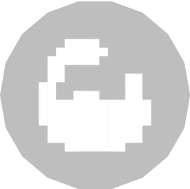
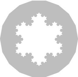
Figure 2. Sketch of a pixelation approximation (left) and pre-fractal approximation (right) of $\Omega$.

2.7. Examples

In [26], we studied the following general approximation scheme, which is able to produce easy-to-triangulate approximations of $U$, converging in the sense of Assumption 2.10, provided we have access to the information of whether a given point $x$ lies inside $U$.

Example 1 (Pixelated domains).

Consider an obstacle $U$ satisfying Assumption 2.9, Define the pixelation approximation of $U$ by (see Figure 2)

(2.42) $$U_{n}:=\bigcup_{j\in L_{n}}(j+[-\tfrac{1}{2n},\tfrac{1}{2n}]^{2}),\qquad n\in\mathbb{N},$$

where

(2.43) $$L_{n}:=\{j\in(\tfrac{1}{n}\mathbb{Z})^{2}:j\in U\}.$$

Then, by [26, Proposition 4.14], Assumption 2.10 for $U_{n}$ holds true.

In addition, many fractals are naturally defined as the Hausdorrf limit of a sequence of polygonal “pre-fractal” sets. In the case where $\partial U$ is such a fractal, one may use these pre-fractals to construct $U_{n}$. As a simple example, consider the Koch snowflake.

Example 2 (Koch snowflake).

Consider the case that the obstacle $U$ is the Koch snowflake, which is defined as the Hausdorrf limit of a sequence of pre-fractals $U_{n}$, as illustrated in Figure 2. The boundary of the Koch snowflake is path-connected since it naturally inherits a parametrisation from the boundaries of the pre-fractals, hence Assumption 2.9 is satisfied. Furthermore, Assumption 2.10 for $U_{n}$ is satisfied, essentially, by construction.

2.8. Structure of paper

Our paper is organised as follows: Section 3: Mosco convergence and Gohberg-Sigal theory are introduced, then slightly more general version of our main result is stated.

Section 4: Theorem 2.13 is proved.

Section 5: Theorem 2.3 is proved.

Section 6: An implementation of the numerical method is described with figures illustrating the scattering resonances of fractal obstacles.

Appendix A: Some necessary properties of the operator $T(k)$ are proved.

Throughout, $C>0$ shall denote a positive constant that may change from line to line and whose dependence shall be indicated throughout unless specified otherwise (e.g. $C_{s,X}(k)$ depends only on $s$, $X$ and $k$).

3. Preliminaries and reformulation of the result

In this section, we collect the necessary tools we require from Mosco convergence and Gohberg-Sigal theory. Following this we shall reformulate the main result slightly and reduce its proof of Proposition 3.15, (which essentially states the locally uniform operator norm convergence of $T_{n}(k)$ to $T(k)$.

3.1. Mosco convergence

The notion of Mosco convergence for Hilbert space plays a central role in our analysis.

Definition 3.1.

Let $\mathcal{W}$ and $\mathcal{W}_{n}$, $n\in\mathbb{N}$, be closed subspaces of a Hilbert space $\mathcal{H}$. We say that $\mathcal{W}_{n}$ converges to $\mathcal{W}$ in the Mosco sense as $n\to\infty$, denoted by $\mathcal{W}_{n}\xrightarrow{M}\mathcal{W}$ as $n\to\infty$, if the following holds:

1. For every $u\in\mathcal{W}$, there exists $u_{n}\in\mathcal{W}_{n}$, $n\in\mathbb{N}$, such that $\lVert u_{n}-u\rVert_{\mathcal{H}}\to 0$ as $n\to\infty$.

2. For every subsequence $(\mathcal{W}_{n_{j}})_{j\in\mathbb{N}}$ of $(\mathcal{W}_{n})_{n\in\mathbb{N}}$, and every sequence $u_{n_{j}}\in\mathcal{W}_{n_{j}}$ with $u_{n_{j}}\rightharpoonup u$ as $j\to\infty$ for some $u\in\mathcal{H}$, we have $u\in\mathcal{W}$.

In [26], we studied the case

(3.1) $$\mathcal{H}=H^{1}(\mathbb{R}^{2}),\quad\mathcal{W}=H^{1}_{0}(\mathcal{O}),\quad\mathcal{W}_{n}=H^{1}_{0}(\mathcal{O}_{n}),$$

where $\mathcal{O}\subset\mathbb{R}^{2}$ and $\mathcal{O}\subset\mathbb{R}^{2}$, $n\in\mathbb{N}$, are bounded domains.

Theorem 3.2 ([26, Theorem 2.3]).

If

1. $\mathcal{O}$ is topologically regular (i.e., $\mathcal{O}=\mathrm{int}(\overline{\mathcal{O}})$),

2. $\partial\mathcal{O}$ has zero Lebesgue measure and a finite number of separated, path-connected components,

3. $\partial\mathcal{O}_{n}$ is locally connected for all $n\in\mathbb{N}$ with

   (3.2) $$\operatorname{dist}_{H}(\mathcal{O},\mathcal{O}_{n})+\operatorname{dist}_{H}(\partial\mathcal{O},\partial\mathcal{O}_{n})\to 0\quad\text{as}\quad n\to\infty,$$

then we have

$$H^{1}_{0}(\mathcal{O}_{n})\xrightarrow{M}H^{1}_{0}(\mathcal{O})\quad\text{as}\quad n\to\infty.$$

An application of this result to the setting in the present paper gives the following result. This is straightforward to verify, however, for the convenience of the reader we provide a proof.

Lemma 3.3.

Assumptions 2.9 and 2.10 imply that

$$H^{1}_{0}(U_{n}^{c})\xrightarrow{M}H^{1}_{0}(U^{c})\quad\text{as}\quad n\to\infty.$$

Proof.

By Theorem 3.2, under Assumptions 2.9 and 2.10, we have

(3.3) $$H^{1}_{0}(B_{X}\backslash U_{n})\xrightarrow{M}H^{1}_{0}(B_{X}\backslash U)\quad\text{as}\quad n\to\infty.$$

Let $(\chi_{1}$, $\chi_{2})$ be a partition of unity for the open cover $(B_{X}$, $\mathbb{R}^{2}\backslash\overline{B}_{X-1})$ of $\mathbb{R}^{2}$. We then necessarily have $\chi_{1}\equiv 1$ on $\overline{B}_{X-1}$. Focusing on Mosco convergence condition (i), let $u\in H^{1}_{0}(U^{c})$. Then there exists $\tilde{u}_{n}\in H^{1}_{0}(B_{x}\backslash U_{n}^{c})$ such that $\tilde{u}_{n}\to\chi_{1}u$ in $H^{1}$, hence $u_{n}:=\tilde{u}_{n}+\chi_{2}u\to\chi_{1}u+\chi_{2}u=u$ in $H^{1}$. Focusing on condition (ii), let $u_{n_{j}}\in H^{1}_{0}(U_{n_{j}}^{c})$, $j\in\mathbb{N}$, such that $u_{n_{j}}\rightharpoonup u$ in $H^{1}$ for some $u\in H^{1}(\mathbb{R}^{2})$. Then $\chi_{1}u_{n_{j}}\rightharpoonup\chi_{1}u$ in $H^{1}$ so $\chi_{1}u\in H^{1}_{0}(B_{X}\backslash U)$. Consequently, $u=\chi_{1}u+\chi_{2}u\in H^{1}_{0}(U^{c})$. ∎

The following lemma shall be used in Lemma 4.10 to establish Mosco convergence properties for $H^{1}_{\textrm{ND}}$ spaces and the associated finite element spaces.

Lemma 3.4 ([7, Lemma 2.4]).

Let $\mathcal{W}$ and $\mathcal{W}_{n}$, $n\in\mathbb{N}$, be closed subspaces of a Hilbert space $\mathcal{H}$. Suppose that the following holds:

1. There exists a dense subspace $\tilde{\mathcal{W}}\subset\mathcal{W}$ such that for every $u\in\tilde{\mathcal{W}}$, there exists a sequence $u_{n}\in\mathcal{W}_{n}$, $n\in\mathbb{N}$, with $\lVert u_{n}-u\rVert_{\mathcal{H}}\to 0$.

2. There exists a sequence of closed subspaces $\mathcal{W}_{n}^{+}$ of $\mathcal{H}$ such that $\mathcal{W}_{n}\subset\mathcal{W}_{n}^{+}$ for all $n$ and $\mathcal{W}_{n}^{+}\xrightarrow{M}\mathcal{W}$.

Then, $\mathcal{W}_{n}\xrightarrow{M}\mathcal{W}$ as $n\to\infty$.

3.2. Gohberg-Sigal theory

Let $\mathcal{X}$ be a Banach space and let $\Sigma\subset\mathbb{C}$ be open. Let $K:\Sigma\to\mathcal{B}(\mathcal{X})$ be an analytic operator-valued function such that $K(z)$ is compact for every $z\in\Sigma$. Then $A(z):=I+K(z)$ is Fredholm of index zero. Furthermore, assume there exists $\tilde{z}\in\Sigma$ such that $A(\tilde{z})$ is invertible. Then by the analytic Fredholm theorem, $z\mapsto A(z)^{-1}$ is a meromorphic operator-valued function on $\Sigma$ with poles of finite rank. These pole exactly coincide with the zeros of $A$, in the sense of the following definition.

Definition 3.5.

Let $\mathcal{X}$ be a Banach space and $\Sigma\subset\mathbb{C}$ be open. The zeros of an analytic operator-valued function $A:\Sigma\to\mathcal{B}(\mathcal{X})$, are defined as the points $z\in\Sigma$ such $\ker A(z)\neq\{0\}$.

The following factorisation theorem is at the heart of Gohberg-Sigal theory and allows us to define a notion of multiplicity to zeros of operator-valued functions. Note that we only state a simplified version here.

Theorem 3.6 ([1, Th. 1.8]).

Let $A$ be as above. Then for any $z_{0}\in\Sigma$, there exists:

1. analytic operator-valued functions $W_{1},W_{2}:\Sigma\to\mathcal{B}(\mathcal{X})$, invertible near $z_{0}$,

2. mutually disjoint projection operators $P_{0},...,P_{M}$ with

   $$\mathrm{rank}P_{j}=1\quad\text{for}\quad 1\leq j\leq M\quad\text{and}\quad P_{0}+\sum_{j=1}^{M}P_{j}=I$$

3. positive integers $l_{1},...,l_{M}$,

such that

$$A(z)=W_{1}(z)\left(P_{0}+\sum_{j=1}^{M}(z-z_{0})^{l_{j}}P_{j}\right)W_{2}(z).$$

Remark 3.7.

Note that the above result follows from [1] because, in the language used there, $z_{0}$ is a normal point of $A$ (cf. [1, Section 1.1.4])

Definition 3.8.

Suppose that $A$ satisfies the hypotheses of Theorem 3.6. The null multiplicity of a zero $z_{0}\in\Sigma$ of $A$ is defined as $l_{1}+\cdots+l_{M}$.

A simplified version of the generalised Rouché’s theorem for operator-valued functions reads as follows.

Theorem 3.9 (Generalised Rouché’s theorem [1, Th. 1.15]).

Let $A_{j}=I+K_{j}:\Sigma\to\mathcal{B}(\mathcal{X})$, $j=1,2$, both satisfy the hypotheses of Theorem 3.6. Let $D\Subset\Sigma$ be a simply connected open set with $C^{1}$ boundary $\partial D$ on which neither $A_{1}$ nor $A_{2}$ has any zeros. If

$$\lVert A_{1}(z)^{-1}\left(A_{1}(z)-A_{2}(z)\right)\rVert<1\quad\text{for all}\quad z\in\partial D,$$

then the number of zeros of $A_{1}$ and $A_{2}$ in $D$ coincide, counting null multiplicities.

Remark 3.10.

Note that the above result follows from [1] because $A_{1}-A_{2}$ is analytic on an open neighbourhood of $\overline{D}$ and, in the language used there, $A_{1}$ is normal with respect to $\partial D$ (cf. [1, Section 1.3.1]).

The following generalisation of Hurwitz’s theorem follows from the above Rouché’s theorem and shall be applied in the proof of our main result.

Lemma 3.11.

Let $A=I+K:\Sigma\to\mathcal{B}(\mathcal{X})$, and $A_{n}=I+K_{n}:\Sigma\to\mathcal{B}()$, $n\in\mathbb{N}$, all satisfy the hypotheses of Theorem 3.6. If we have

(3.4) $$\lVert A(z)-A_{n}(z)\rVert\to 0\quad\text{as}\quad n\to\infty\qquad\text{locally uniformly for}\qquad z\in\Sigma,$$

then the following holds.

1. For any zero $w$ of $A$ with null multiplicity $\nu$, there exists $n_{0}\in\mathbb{N}$ and $\nu$ sequences of zeros $w^{(1)}_{n},...,w^{(\nu)}_{n}$, $n\geq n_{0}$, of $A_{n}$ such that $w^{(j)}_{n}\to w$ as $n\to\infty$ for all $j\in\{1,...,\nu\}$

2. For any bounded, open subset $D\Subset\Sigma$ not containing any zeros of $A$, there exists $n_{0}\in\mathbb{N}$ such that $A_{n}$ has no zeros in $D$ for all $n\geq n_{0}$.

Proof.

First, focus on (a). Let $w$ be a zero of $A$. Since $A$ is analytic, there exists $\varepsilon_{0}>0$ such that $\overline{B_{\varepsilon_{0}}(w)}$ intersects neither $\partial\Sigma$ nor any other zero of $A$. Let $\varepsilon\in(0,\varepsilon_{0})$. There exists $C>0$ such that for all $n\in\mathbb{N}$,

$$\sup_{|z-w|=\varepsilon}\lVert A(z)^{-1}\left(A(z)-A_{n}(z)\right)\rVert\leq C\sup_{|z-w|=\varepsilon}\lVert A(z)-A_{n}(z)\rVert$$

hence, by the hypothesis (3.4) and the generalised Rouché’s theorem, there exists $n_{1}(\varepsilon)\in\mathbb{N}$ such that $A_{n}$ has $\nu$ zeroes in $B_{\varepsilon}(w)$ for all $n\geq n_{1}(\varepsilon)$. The proof of (a) is completed by setting $n_{0}=n_{1}(\varepsilon)$.

Next, we prove (b). Let $D_{1},...,D_{N}\subseteq D$ be a collection of simply connected, bounded open sets such that $\cup_{j=1}^{N}D_{j}=D$. By the same argument used to prove (a), for each $j\in\{1,...,N\}$, there exists $n_{j}\in\mathbb{N}$ such that $A_{n}$ does not have any zeros in $D_{j}$ for all $n\geq n_{j}$. The proof of (b) is completed by setting $n_{0}=\max\{n_{1},...,n_{N}\}$. ∎

In addition, we shall need the following lemma, which will be used to verify the uniform convergence hypothesis of the above generalised Hurwitz’s theorem.

Lemma 3.12.

Let $D\subset\mathbb{C}$ be a convex, bounded Cauchy domain (cf. [27, p. 268]) and let $A,A_{n}:D\to\mathcal{B}(\mathcal{X})$, $n\in\mathbb{N}$, be analytic operator-valued functions. Assume that

1. $\|A_{n}(z)-A(z)\|\to 0$ as $n\to\infty$ for all $z\in D$,

2. $\sup_{n\in\mathbb{N}}\sup_{z\in D}\|A_{n}(z)\|<+\infty$.

then

$$\sup_{z\in Q}\|A_{n}(z)-A(z)\|\to 0\quad\text{ as }n\to\infty$$

for any compact $Q\subset D$.

Proof.

For $z,w\in\mathbb{C}$ the notation $[z,w]$ denoted the line segment connecting $z$ to $w$. The strategy of the proof is to prove equicontinuity of the sequence $(\|A_{n}\|)_{n\in\mathbb{N}}$ and then use the Arzelá-Ascoli theorem (note that boundedness already follows from the assumptions).

For convenience we denote $C_{n}:=A_{n}-A$ and

$$f_{n}(z):=\|C_{n}(z)\|.$$

in the rest of the proof. For $z,w\in D$ one has

(3.5) $$|f_{n}(z)-f_{n}(w)|\leq\|C_{n}(w)-C_{n}(z)\|=\biggl{\|}\int_{[z,w]}\frac{dC_{n}}{dz}(\tilde{w})\,d\tilde{w}\biggr{\|}\leq|z-w|\biggl{\|}\frac{dC_{n}}{dz}(\cdot)\biggr{\|}_{L^{\infty}([z,w];\mathcal{B}(\mathcal{X}))}$$

for all $n\in\mathbb{N}$. Note that convexity of $D$ implies $[z,w]\subset\operatorname{conv}(Q)\Subset D$. Since $w\mapsto\big{\|}\frac{dC_{n}}{dz}(w)\big{\|}$ is continuous, it has a maximum on $[z,w]$, say

(3.6) $$\biggl{\|}\frac{dC_{n}}{dz}(\cdot)\biggr{\|}_{L^{\infty}([z,w];\mathcal{B}(\mathcal{X}))}=\biggl{\|}\frac{dC_{n}}{dz}(\zeta_{n})\biggr{\|}.$$

The openness of $D$ and the fact that $\{\zeta_{n}\}_{n\in\mathbb{N}}\Subset D$ imply that $r:=\inf_{n\in\mathbb{N}}\operatorname{dist}(\zeta_{n},\partial B)>0$. By Cauchy’s integral formula for operator-valued functions (cf. [27, Th. V.1.4]) one has

$$\frac{dC_{n}}{dz}(\zeta_{n})=\frac{1}{2\pi i}\oint_{\partial D}\frac{C_{n}(w)}{(\zeta_{n}-w)^{2}}\,dw.$$

Taking norms on both sides, we obtain

(3.7) $$\biggl{\|}\frac{dC_{n}}{dz}(\zeta_{n})\biggr{\|}\leq\frac{1}{2\pi}\oint_{\partial D}\frac{\|C_{n}(w)\|}{|\zeta_{n}-w|^{2}}\,dw\leq\frac{|\partial D|}{r^{2}}\|C_{n}\|_{L^{\infty}(D;\mathcal{B}(\mathcal{X}))},$$

where $|\partial D|$ denotes the arc length of $\partial D$. By boundedness of $\|A_{n}\|$ (assumption (ii)) and (3.7) we have

(3.8) $$\sup_{n\in\mathbb{N}}\biggl{\|}\frac{dC_{n}}{dz}(\zeta_{n})\biggr{\|}\leq\frac{|\partial D|}{r^{2}}\sup_{n\in\mathbb{N}}\|C_{n}\|_{L^{\infty}(\gamma_{n};\mathcal{B}(\mathcal{X}))}<+\infty.$$

Combining eqs. (3.5)-(3.8) we conclude that

$$|f_{n}(z)-f_{n}(w)|\leq C|z-w|$$

for all $z,w\in Q$ and all $n\in\mathbb{N}$, hence the set $\{f_{n}|_{Q}\}_{n\in\mathbb{N}}$ is equicontinuous. Applying the Arzelá-Ascoli theorem we conclude that there exists a subsequence $(f_{n_{k}})_{k\in\mathbb{N}}$, which converges uniformly on $Q$. By pointwise convergence of the $A_{n}$ (assumption (i)) the limit is identified as 0, i.e. $f_{n_{k}}\to 0$ uniformly on $Q$. Finally, applying the same reasoning to every subsequence of $(f_{n})_{n\in\mathbb{N}}$ we conclude that $f_{n}\to 0$ uniformly on $Q$. ∎

Finally, in order to apply Gohberg-Sigal theory to our setting, we require that the operator-valued functions $T$ and $T_{n}$ admit decompositions as the sum of the identity and a compact operator on $L^{2}(\Gamma)$. In fact, this does not hold for $T_{n}$ since it is finite-rank, however, we may easily overcome this by introducing an auxiliary operator-valued function

(3.9) $$\tilde{T}_{n}(k):=(I-P_{n})+T_{n}(k),\qquad n\in\mathbb{N},\quad k\in\mathbb{C}_{-}$$

whose zeros coincide with $T_{n}$. On the other hand, the desired decomposition for $T$ is proven in Appendix A.

Proposition 3.13.

Consider the operator-valued function $T:\mathbb{C}_{-}\to\mathcal{B}(L^{2}(\Gamma))$ defined by (2.21). There exists an analytic compact-operator-valued function $K:\mathbb{C}_{-}\to\mathcal{K}(L^{2}(\Gamma))$ such that

$$T(k)=I+K(k),\qquad k\in\mathbb{C}_{-}.$$

3.3. Reformulation of Theorem 2.13

We are now in a position to state a slight generalisation of Theorem 2.13. This generalisation takes into account the algebraic multiplicities of the resonances, which are defined as follows.

Definition 3.14.

The algebraic multiplicity of a scattering resonance $k\in\mathbb{C}_{-}$ of $H$ is defined as the null multiplicity of the corresponding zero of the operator-valued function $T:\mathbb{C}_{-}\to\mathcal{B}(L^{2}(\Gamma))$ defined by (2.21).

Theorem 2.13 follows immediately from next theorem by Lemma 3.3.

Theorem 2.13’.

Suppose that Assumptions 2.10-2.12 hold and

$$H^{1}_{0}(U_{n}^{c})\xrightarrow{M}H^{1}_{0}(U^{c})\quad\text{as}\quad n\to\infty.$$

1. For any resonance $k\in\mathbb{C}_{-}$ of $H$ with algebraic multiplicity $\nu$, there exists $n_{0}\in\mathbb{N}$ and $\nu$ sequences of zeros $k^{(1)}_{n},...,k^{(\nu)}_{n}\in\mathbb{C}_{-}$ of $g_{n}$, $n\geq n_{0}$, such that $k^{(j)}_{n}\to k$ as $n\to\infty$ for all $j\in\mathbb{C}_{-}$.

2. For any bounded, open subset $D\subset\mathbb{C}_{-}$ such that $\overline{D}$ does not contain any resonances of $H$, there exists $n_{0}\in\mathbb{N}$ such that $D$ does not contain any zeros of $T_{n}$ for any $n\geq n_{0}$.

The purpose of Section 4 shall be to prove the following result regarding the convergence and uniform boundedness of the sequence of numerical approximations $T_{n}(k)$, $n\in\mathbb{N}$.

Proposition 3.15.

Let $T:\mathbb{C}_{-}\to\mathcal{B}(L^{2}(\Gamma))$ and $\tilde{T}_{n}:\mathbb{C}_{-}\to\mathcal{B}(L^{2}(\Gamma))$, $n\in\mathbb{N}$, be the operator-valued functions defined by (2.21) and (3.9) respectively. Suppose that Assumptions 2.10-2.12 hold and

$$H^{1}_{0}(U_{n}^{c})\xrightarrow{M}H^{1}_{0}(U^{c})\quad\text{as}\quad n\to\infty.$$

Then the following holds.

1. $\|\tilde{T}_{n}(k)-T(k)\|_{L^{2}\to L^{2}}\to 0$ as $n\to\infty$ for all $k\in\mathbb{C}_{-}$,

2. $\sup_{n\in\mathbb{N}}\sup_{k\in D}\|\tilde{T}_{n}(k)\|_{L^{2}\to L^{2}}<+\infty$ for every bounded set $D\subset\mathbb{C}_{-}$ with $\overline{D}\subset\mathbb{C}_{-}$.

As we shall now show, the main result follows from this proposition.

Proof of Theorem 2.13’.

By Proposition 3.15 and Lemma 3.12, we have $\lVert\tilde{T}_{n}(k)-T(k)\rVert_{L^{2}\to L^{2}}\to 0$ as $n\to\infty$ locally uniformly for $k\in\mathbb{C}_{-}$. The result then follows by an application of the generalised Hurwitz’s result Lemma 3.11. ∎

4. Main convergence proof

In this section, we prove Theorem 2.13 which, as shown above, amounts to proving Proposition 3.15. In Subsection 4.1, we begin by estimating the full error term $\lVert T(k)-\tilde{T}_{n}(k)\rVert_{L^{2}\to L^{2}}$ from Proposition 3.15 (a) in terms of three other terms which, respectively, isolate the error arising from matrix truncation, sum truncation in the eigenfunction expansion and the error from the finite element method (including the polygonal approximation of boundaries). Subsection 4.2 then develops several necessary tools. The matrix and sum truncation error are dealt with in in Subsection 4.3 while the finite element error is dealt with in Subsection 4.4. The proof is concluded in Subsection 4.5.

4.1. Initial estimates

Let us first introduce three operators that will play a key role in our analysis.

• Define an FEM space on the boundary $\Gamma_{n}$ as follows,

  $$V^{n}(\Gamma_{n}):=\left\{u|_{\Gamma_{n}}:u\in V^{n}(\Omega_{n})\right\}.$$

  We let

  (4.1) $$\hat{\Pi}_{n}:C(\Gamma)\to V^{n}(\Gamma_{n})$$

  denote a linear interpolation operator on $\Gamma$, which is defined as one would expect: $\hat{\Pi}_{n}g$ is the unique function in $V^{n}(\Gamma_{n})$ such that $(\hat{\Pi}_{n}g)(p)=g(p)$ for any $p\in\Gamma\cap\Gamma_{n}$

• For each $k\in\mathbb{C}_{-}$, the operator

  $$S(k)\in\mathcal{B}(H^{-\frac{1}{2}}(\Gamma);H^{1}_{\mathrm{ND}}(\Omega))$$

  is defined as the weak solution operator for the boundary value problem (2.15) associated to $M_{\mathrm{in}}(k)$. In other words, for any $g\in H^{-\frac{1}{2}}(\Gamma)$, $u=S(k)g$ solves

  (4.2) $$u\in H^{1}_{\mathrm{ND}}(\Omega):\qquad\langle\nabla u,\nabla\phi\rangle_{L^{2}(\Omega)}=k^{2}\langle u,\phi\rangle_{L^{2}(\Omega)}+(g,\phi|_{\Gamma})_{H^{-\frac{1}{2}},H^{\frac{1}{2}}},\qquad\forall\phi\in H^{1}_{\mathrm{ND}}(\Omega).$$

  Note that we have

  (4.3) $$M_{\mathrm{in}}(k)=\gamma_{\Gamma}S(k),\qquad k\in\mathbb{C}_{-}.$$

• Furthermore, we introduce an FEM discretisation

  $$S_{n}(k)\in\mathcal{B}(P_{n}H^{-\frac{1}{2}}(\Gamma);V^{n}_{\mathrm{ND}}(\Omega_{n}))$$

  of $S(k)$ as in (2.31), that is, given $g\in P_{n}H^{-\frac{1}{2}}(\Gamma)$, $u_{n}=S_{n}(k)g$ solves

  (4.4) $$u_{n}\in V^{n}_{\mathrm{ND}}(\Omega_{n}):\qquad\langle\nabla u_{n},\nabla\phi\rangle_{L^{2}(\Omega_{n})}=k_{0}^{2}\langle u_{n},\phi\rangle_{L^{2}(\Omega_{n})}+(\hat{\Pi}_{n}g,\phi|_{\Gamma_{n}})_{L^{2}(\Gamma_{n})},\qquad\forall\phi\in V^{n}_{\mathrm{ND}}(\Omega_{n}).$$

  Note that in terms of the approximation $\hat{M}^{n}_{\mathrm{in}}(k)$ for the inner NtD map introduced in Section 2, we have

  $$\hat{M}^{n}_{\mathrm{in}}(k)=\gamma_{\Gamma_{n}}S_{n}(k),\qquad k\in\mathbb{C}_{-},\quad n\in\mathbb{N}.$$

In what follows, it shall be helpful to consider intermediate sequence of operators $\hat{\Pi}^{*}_{n}\gamma_{\Gamma_{n}}\hat{M}^{n}_{\mathrm{in}}(k)$, $n\in\mathbb{N}$, on $L^{2}(\Gamma)$. Here, $\hat{\Pi}_{n}^{*}$ denotes the adjoint of the interpolation operator $\hat{\Pi}_{n}$ (i.e., so that the matrix elements of $\hat{\Pi}^{*}_{n}\hat{M}^{n}_{\mathrm{in}}(k)$ are given by $(\hat{M}^{n}_{\mathrm{in}}(k)e_{\alpha},\hat{\Pi}_{n}e_{\beta})_{L^{2}(\Gamma_{n})}$).

The three sources of error are as follows.

• The matrix truncation error is defined by

  (4.5) $$\mathcal{E}^{n}_{\mathrm{mat}}(k):=\lVert K(k)-P_{n}K(k)P_{n}\rVert_{L^{2}\to L^{2}}$$

  where $K(k)$ is the family of compact operators from Proposition 3.13.

• The sum truncation error is defined by

  (4.6) $$\mathcal{E}^{n}_{\mathrm{sum}}(k):=\lVert P_{n}(\hat{\Pi}_{n}^{*}\hat{M}^{n}_{\mathrm{in}}(k)-M_{\mathrm{in}}^{n}(k))P_{n}\rVert_{H^{-\frac{1}{2}}\to H^{\frac{1}{2}}}.$$

• The finite element error is defined by

  (4.7) $$\mathcal{E}^{n}_{\mathrm{sol}}(k):=\lVert P_{n}(M_{\mathrm{in}}(k)-\hat{\Pi}_{n}^{*}\hat{M}^{n}_{\mathrm{in}}(k))P_{n}\rVert_{H^{-\frac{1}{2}}\to H^{\frac{1}{2}}}.$$

We have the following estimate.

Lemma 4.1.

For all $k\in\mathbb{C}_{-}$ and $n\in\mathbb{N}$, it holds that

$$\lVert T(k)-\tilde{T}_{n}(k)\rVert_{L^{2}\to L^{2}}\leq\mathcal{E}^{n}_{\mathrm{mat}}(k)+C_{X}(k)\left(\mathcal{E}^{n}_{\mathrm{sum}}(k)+\mathcal{E}^{n}_{\mathrm{sol}}(k)\right),$$

for some locally uniform constant $C_{X}(k)>0$.

Proof.

First, adding and subtracting $I+P_{n}K(k)P_{n}$,

$$\lVert T(k)-\tilde{T}_{n}(k)\rVert_{L^{2}\to L^{2}}\leq\underbrace{\lVert T(k)-(I+P_{n}K(k)P_{n})\rVert_{L^{2}\to L^{2}}}_{=\mathcal{E}^{n}_{\mathrm{mat}}(k)}+\lVert(I+P_{n}K(k)P_{n})-\tilde{T}_{n}(k)\rVert_{L^{2}\to L^{2}}$$

where we have recognised the first term on the right hand side to be $\mathcal{E}^{n}_{\mathrm{mat}}(k)$ since $T(k)=I+K(k)$. The second term may be simplified using the definitions of $\tilde{T}_{n}(k)$, $T_{n}(k)$ and $T(k)$, as well as the locally uniform boundedness of $N_{2}(k)$ between $H^{\frac{1}{2}}$ and $H^{-\frac{1}{2}}$,

$$\lVert(I+P_{n}K(k)P_{n})-\tilde{T}_{n}(k)\rVert_{L^{2}\to L^{2}} =\lVert P_{n}T(k)P_{n}-T_{n}(k)\rVert_{L^{2}\to L^{2}}$$

$$=\tfrac{1}{2}\lVert\mathcal{N}^{\frac{1}{2}}P_{n}(M_{\mathrm{in}}(k)-M_{\mathrm{in}}^{n}(k))P_{n}N_{2}(k)\mathcal{N}^{-\frac{1}{2}}\rVert_{L^{2}\to L^{2}}$$

$$=C_{X}(k)\lVert P_{n}(M_{\mathrm{in}}(k)-M_{\mathrm{in}}^{n}(k))P_{n}\rVert_{H^{-\frac{1}{2}}\to H^{\frac{1}{2}}}.$$

The proof is complete by adding and subtracting $\hat{\Pi}_{n}^{*}\hat{M}^{n}_{\mathrm{in}}(k)$ as follows,

$$\lVert P_{n}(M_{\mathrm{in}}(k)-M_{\mathrm{in}}^{n}(k))P_{n}\rVert_{H^{-\frac{1}{2}}\to H^{\frac{1}{2}}}\\ \leq\underbrace{\lVert P_{n}(\hat{\Pi}_{n}^{*}\hat{M}^{n}_{\mathrm{in}}(k)-M_{\mathrm{in}}^{n}(k))P_{n}\rVert_{H^{-\frac{1}{2}}\to H^{\frac{1}{2}}}}_{=\mathcal{E}^{n}_{\mathrm{sum}}(k)}+\underbrace{\lVert P_{n}(M_{\mathrm{in}}(k)-\hat{\Pi}_{n}^{*}\hat{M}^{n}_{\mathrm{in}}(k))P_{n}\rVert_{H^{-\frac{1}{2}}\to H^{\frac{1}{2}}}}_{=\mathcal{E}^{n}_{\mathrm{sol}}(k)}.$$

∎

4.2. Bijection, interpolation and extension operators

In this section, we collect some tools that we require, namely the following:

• (Lemma 4.2) In order to compare functions on the interface $\Gamma$ with the polygonal approximation of the interface $\Gamma_{n}$, we shall use bijection operators

  $$\hat{\iota}_{n}:C(\Gamma_{n})\to C(\Gamma),\qquad n\in\mathbb{N}.$$

• (Lemma 4.3) In order to compare piecewise affine functions on $\Omega_{n}$ with functions on $\Omega$ we shall use extension operators

  $$E_{n}:V^{n}_{\mathrm{ND}}(\Omega_{n})\to H^{1}(B_{X}),\qquad n\in\mathbb{N}.$$

• (Lemma 4.4) We shall need certain Sobolev norm estimates for the boundary linear interpolation operator $\hat{\Pi}_{n}$.

• (Lemma 4.5) Finally, we need uniform (in $n$) Sobolev norm estimates for the trace operator $\gamma_{\Gamma_{n}}$.

First, we construct the bijection operators $\hat{\iota}_{n}$.

Lemma 4.2.

There exists a sequence of invertible maps $\hat{\iota}_{n}:C(\Gamma_{n})\to C(\Gamma)$, $n\in\mathbb{N}$, such that:

1. $(\hat{\iota}_{n}g)(p)=g(p)$ for any point $p\in\Gamma\cap\Gamma_{n}$, $n\in\mathbb{N}$ and $g\in C(\Gamma_{n})$,

2. There exists a sequence $\delta_{X}(n)>0$, $n\in\mathbb{N}$, with $\lim_{n\to\infty}\delta_{X}(n)=0$ such that for any $s\geq 0$, $(g_{n}^{(1)})_{n\in\mathbb{N}}\subset C(\Gamma_{n})\cap H^{-s}(\Gamma_{n})$ and $(g_{n}^{(2)})_{n\in\mathbb{N}}\subset C(\Gamma_{n})\cap H^{s}(\Gamma_{n})$, we have

   $$\left\lvert(\hat{\iota}_{n}g_{n}^{(1)},\hat{\iota}_{n}g_{n}^{(2)})_{L^{2}(\Gamma)}-(g_{n}^{(1)},g_{n}^{(2)})_{L^{2}(\Gamma_{n})}\right\rvert\leq\delta_{X}(n)\lVert g_{n}^{(1)}\rVert_{H^{-s}(\Gamma_{n})}\lVert g_{n}^{(2)}\rVert_{H^{s}(\Gamma_{n})},\qquad n\in\mathbb{N}.$$

3. For any $s\in[0,1]$, we have

   $$\sup_{n\in\mathbb{N}}\,\lVert\hat{\iota}_{n}\rVert_{H^{s}\to H^{s}}<\infty\qquad\text{and}\qquad\sup_{n\in\mathbb{N}}\,\lVert\hat{\iota}^{-1}_{n}\rVert_{H^{s}\to H^{s}}<\infty.$$

Proof.

Recall that $\Gamma=\partial B_{X}(0)$ and , for each $n\in\mathbb{N}$, $\Gamma_{n}=\partial B_{X}^{n}$, where $B_{X}^{n}$ is convex with $\{0\}\in B_{X}^{n}\subset B_{X}(0)$. Therefore, there exists a unique Lipschitz bijection $\iota_{n}:\Gamma\to\Gamma_{n}$ such that, for any $p\in\Gamma$, $\iota_{n}(p)$ is the unique point in $\Gamma_{n}$ with the same angular coordinate as $p$. Define

(4.8) $$\hat{\iota}_{n}g=g\circ\iota_{n},\qquad g\in C(\Gamma_{n}).$$

Then, (a) clearly holds.

Focus on (b). Let $s\geq 0$. Let $(g_{n}^{(1)})_{n\in\mathbb{N}}\subset C(\Gamma_{n})$ be bounded in $H^{-s}(\Gamma_{n})$ and let $(g_{n}^{(2)})_{n\in\mathbb{N}}\subset C(\Gamma_{n})$ be bounded in $H^{s}(\Gamma)$. By a change of variables,

$$(\hat{\iota}_{n}g_{n}^{(1)},\hat{\iota}_{n}g_{n}^{(2)})_{L^{2}(\Gamma)}=\int_{\Gamma}g_{n}^{(1)}(\iota_{n}(\theta))\overline{g_{n}^{(2)}}(\iota_{n}(\theta))\,\mathrm{d}\theta=\int_{\Gamma_{n}}g_{n}^{(1)}(t)\overline{g_{n}^{(2)}}(t)\frac{\mathrm{d}\iota_{n}^{-1}}{\mathrm{d}t}(t)\,\mathrm{d}t.$$

Consequently, we have

$$\left\lvert(\hat{\iota}_{n}g_{n}^{(1)},\hat{\iota}_{n}g_{n}^{(2)})_{L^{2}(\Gamma)}-(g_{n}^{(1)},g_{n}^{(2)})_{L^{2}(\Gamma_{n})}\right\rvert =\left\lvert\left((1-\frac{\mathrm{d}\iota_{n}^{-1}}{\mathrm{d}t})g_{n}^{(1)},g_{n}^{(2)})\right)_{L^{2}(\Gamma_{n})}\right\rvert$$

$$\leq\lVert(1-\frac{\mathrm{d}\iota_{n}^{-1}}{\mathrm{d}t})g_{n}^{(1)}\rVert_{H^{-s}(\Gamma_{n})}\lVert g_{n}^{(2)}\rVert_{H^{s}(\Gamma_{n})}$$

$$\leq\lVert 1-\frac{\mathrm{d}\iota_{n}^{-1}}{\mathrm{d}t}\rVert_{L^{\infty}(\Gamma_{n})}\lVert g_{n}^{(1)}\rVert_{H^{-s}(\Gamma_{n})}\lVert g_{n}^{(2)}\rVert_{H^{s}(\Gamma_{n})}.$$

It can be directly verified that $\tfrac{\mathrm{d}\iota_{n}^{-1}}{\mathrm{d}t}\to 1$ as $n\to\infty$ pointwise, completing the proof.

Finally, focus on (c). We shall only prove the statement for $\hat{\iota}^{-1}_{n}$; the proof of the statement for $\hat{\iota}_{n}$ is very similar. The case $s=0$ follows directly from (b) so it suffices to show that

(4.9) $$[\hat{\iota}_{n}^{-1}u]_{H^{s}(\Gamma_{n})}\leq C_{X}[u]_{H^{s}(\Gamma)},\qquad n\in\mathbb{N},\quad u\in H^{s}(\Gamma),$$

for $s\in(0,1)$, where $[\cdot]_{H^{s}(\Gamma)}$ and $[\cdot]_{H^{s}(\Gamma_{n})}$ denote the respective $H^{s}$ semi-norms. By the Gagliardo representation for the semi-norms $[\cdot]_{H^{s}(\Gamma)}$, we have

(4.10) $$[\hat{\iota}_{n}^{-1}u]^{2}_{H^{s}(\Gamma_{n})}\leq C_{X}\int_{\Gamma_{n}}\int_{\Gamma_{n}}\frac{|u(\iota_{n}^{-1}(x))-u(\iota_{n}^{-1}(y))|^{2}}{|x-y|^{1+2s}}\,\mathrm{d}x\mathrm{d}y.$$

Performing a change of variables, we have

$$\int_{\Gamma_{n}}\int_{\Gamma_{n}} \frac{|u(\iota_{n}^{-1}(x))-u(\iota_{n}^{-1}(y))|^{2}}{|x-y|^{1+2s}}\,\mathrm{d}x\mathrm{d}y=\int_{\Gamma}\int_{\Gamma}\frac{|u(\theta)-u(\phi)|^{2}}{|\iota_{n}(\theta)-\iota_{n}(\phi)|^{1+2s}}\frac{\mathrm{d}\iota_{n}}{\mathrm{d}\theta}(\theta)\frac{\mathrm{d}\iota_{n}}{\mathrm{d}\phi}(\phi)\,\mathrm{d}\theta\mathrm{d}\phi$$

$$\leq\lVert\iota_{n}\rVert^{2}_{W^{1,\infty}(\Gamma)}\left(\sup_{\theta,\phi\in\Gamma}\frac{|\theta-\phi|}{|\iota_{n}(\theta)-\iota_{n}(\phi)|}\right)^{1+2s}\int_{\Gamma}\int_{\Gamma}\frac{|u(\theta)-u(\phi)|^{2}}{|\theta-\phi|^{1+2s}}\,\mathrm{d}\theta\mathrm{d}\phi$$

(4.11) $$\leq C_{X}\left(\sup_{\theta,\phi\in\Gamma}\frac{|\theta-\phi|}{|\iota_{n}(\theta)-\iota_{n}(\phi)|}\right)^{1+2s}[u]^{2}_{H^{s}(\Gamma)}$$

where the last line follows by again using the Gagliardo representation for the $H^{s}$ semi-norm, as well as the fact that $\lVert\iota_{n}\rVert_{W^{1,\infty}(\Gamma)}\leq C_{X}$. Finally, the term in the brackets on the right hand side of (4.2) is estimated as

(4.12) $$\sup_{\theta,\phi\in\Gamma}\frac{|\theta-\phi|}{|\iota_{n}(\theta)-\iota_{n}(\phi)|}=\sup_{x,y\in\Gamma_{n}}\frac{|\iota_{n}^{-1}(x)-\iota_{n}^{-1}(y)|}{|x-y|}\leq C_{X}\lVert\iota_{n}^{-1}\rVert_{W^{1,\infty}(\Gamma_{n})}\leq C_{X},$$

where the third line holds by Taylor’s theorem. Substituting (4.12) into the right hand side of (4.2), we obtain a constant independent of $s$ by take a supremum over $s\in(0,1)$, completing the proof.

∎

Next, we construct the aforementioned extension operators $E_{n}$.

Lemma 4.3.

There exists a sequence of operators $E_{n}:V^{n}_{\mathrm{ND}}(\Omega_{n})\to H^{1}(B_{X})$, $n\in\mathbb{N}$, such that:

1. $E_{n}u=u$ on $\Omega_{n}$ for any $u\in V^{n}_{\mathrm{ND}}(\Omega_{n})$ and $n\in\mathbb{N}$,

2. $\sup_{n\in\mathbb{N}}\lVert E_{n}\rVert_{H^{1}\to H^{1}}<\infty$,

3. $\hat{\iota}_{n}u|_{\Gamma_{n}}=(E_{n}u)|_{\Gamma}$ for every $n\in\mathbb{N}$ and $u\in V^{n}_{\mathrm{ND}}(\Omega_{n})$.

Proof.

Let $\mathcal{T}_{n}^{\partial}$ denote the set of elements $T\in\mathcal{T}_{n}$ with an edge lying in $\Gamma_{n}$. For any $T\in\mathcal{T}_{n}^{\partial}$, let $I_{T}$ denote the open region enclosed between $T$ and $\Gamma$, so that $B_{X}$ may be decomposed as

$$B_{X}=\mathrm{int}(\overline{B}_{X}^{n}\cup\bigg{(}\bigcup_{T\in\mathcal{T}_{n}^{\partial}}I_{T}\bigg{)}).$$

Let $n\in\mathbb{N}$ and $u\in V^{n}_{\mathrm{ND}}(\Omega_{n})$. Define $E_{n}u$ on $B_{X}^{n}$ by

(4.13) $$E_{n}u|_{B_{X}^{n}}=\begin{cases}u&\text{on }\Omega_{n}\\ 0&\text{on }U_{n}\end{cases}.$$

Furthermore, for any $T\in\mathcal{T}_{n}^{\partial}$, define $E_{n}u$ on $I_{T}$ by

(4.14) $$E_{n}u(p)=u(\iota_{n}(p)),\qquad p\in I_{n}(p),$$

where $\iota_{n}(p)$ is defined as the unique point on $\Gamma_{n}$ with the same angular coordinate as $p$.

Property (a) holds by construction. Furthermore, the map $\iota_{n}$ defined here coincides with $\iota_{n}$ from the proof of Lemma 4.2, hence property (c) also holds.

Let $T\in\mathcal{T}_{n}^{\partial}$. Let $p_{1}$ and $p_{2}$ denote the two points of intersection between $I_{T}$ and $\Gamma$. Since $E_{n}u$ is radial on $I_{T}$, we have

$$\lvert\nabla E_{n}u|_{I_{T}}\rvert=\left\lvert\frac{p_{1}-p_{2}}{|p_{1}-p_{2}|}\cdot\nabla E_{n}u|_{I_{T}}\right\rvert=\left\lvert\frac{p_{1}-p_{2}}{|p_{1}-p_{2}|}\cdot\nabla u|_{T}\right\rvert\leq|\nabla u|_{T}|.$$

where the second equality holds since $\nabla u$ is constant on $T$ and $(p_{1}-p_{2})\nabla u|_{T}$ only depends on $u(p_{1})$ and $u(p_{2})$. Furthermore, by Taylor’s theorem,

$$|u(p)|\leq|u(q)|+X|\nabla u|_{T}|,\qquad p\in I_{T},$$

where $q$ is the reflection of $p$ with respect to the edge of $T$ connecting $p_{1}$ and $p_{2}$. Consequently, we have

(4.15) $$\lVert E_{n}u\rVert_{H^{1}(I_{T})}\leq C_{X}\lVert u\rVert_{H^{1}(T)}.$$

Combining (4.15) with (4.13), we obtain

(4.16) $$\lVert E_{n}u\rVert_{H^{1}(B_{X})}\leq C_{X}\lVert u\rVert_{H^{1}(\Omega_{n})},$$

proving the final required property (b). ∎

We have the following estimate for the boundary linear interpolation operator $\hat{\Pi}_{n}$.

Lemma 4.4.

For any $s\geq 0$, there exists a constant $C_{s,X}>0$ such that for any $n\in\mathbb{N}$, we have

$$\lVert\hat{\iota}_{n}\hat{\Pi}_{n}P_{n}g-g\rVert_{H^{-s}(\Gamma)}\leq C_{s,X}h^{2}_{n}N^{2+s}_{n}\lVert g\rVert_{H^{-s}(\Gamma)},\qquad g\in H^{-s}(\Gamma)$$

and

$$\lVert\hat{\Pi}_{n}P_{n}g\rVert_{H^{-s}(\Gamma_{n})}\leq C_{s,X}(1+h_{n}^{2}N^{2+s}_{n})\lVert g\rVert_{H^{-s}(\Gamma)},\qquad g\in H^{-s}(\Gamma).$$

Proof.

Firstly, we may assume without loss of generality that $g\in P_{n}H^{-s}(\Gamma)\subset C^{\infty}(\Gamma)$. Then, by Lemma 4.2 (c), it suffices to prove that

$$\lVert(\hat{\Pi}_{n}-\hat{\iota}_{n}^{-1})g\rVert_{H^{-s}(\Gamma_{n})}\leq C_{s,X}h_{n}N^{1+s/2}_{n}\lVert g\rVert_{H^{-s}(\Gamma)}.$$

We shall first estimate the left hand side as

$$\lVert(\hat{\Pi}_{n}-\hat{\iota}_{n}^{-1})g\rVert_{H^{-s}(\Gamma_{n})}\leq\lVert(\hat{\Pi}_{n}-\hat{\iota}_{n}^{-1})g\rVert_{L^{2}(\Gamma_{n})}.$$

Let $e\subset\Gamma_{n}$ be any edge joining two adjacent points of contact $p_{1}$ and $p_{2}$ between $\Gamma$ and $\Gamma_{n}$. It suffices to prove

(4.17) $$\lVert(\hat{\Pi}_{n}-\hat{\iota}_{n}^{-1})g\rVert_{L^{2}(e)}\leq C_{s,X}h_{n}N^{1+s/2}_{n}\lVert g\rVert_{H^{-s}(\hat{e})}$$

where $\hat{e}:=\iota_{n}^{-1}(e))$ for the bijection $\iota_{n}:\Gamma\to\Gamma_{n}$ from the proof of Lemma 4.2. Note that $\iota_{n}|_{\hat{e}}$ and $\iota^{-1}_{n}|_{e}$ are smooth and have uniformly bounded $W^{2,\infty}$ norms.

On $e$, we may express $\hat{\Pi}_{n}g$ as

(4.18) $$\hat{\Pi}_{n}g(p)=g(p_{1})\frac{|p-p_{2}|}{|p_{2}-p_{1}|}+g(p_{2})\frac{|p-p_{1}|}{|p_{2}-p_{1}|}.$$

Let $D$ denote the derivative in the direction $p_{2}-p_{1}$.

$$D:=\frac{p_{2}-p_{1}}{|p_{2}-p_{2}|}\cdot\nabla$$

Then,

(4.19) $$D\hat{\Pi}_{n}g(t)=\frac{g(p_{2})-g(p_{1})}{|p_{2}-p_{1}|}.$$

Since $p_{1}$ lies in both $\Gamma$ and $\Gamma_{n}$, we have $\hat{\iota}_{n}^{-1}g(p_{1})=\hat{\Pi}_{n}g(p_{1})=g(p_{1})$. Therefore,

$$|(\hat{\iota}_{n}^{-1}-\hat{\Pi}_{n})g(p)| \leq\int_{e}\left\lvert\frac{g(p_{2})-g(p_{1})}{|p_{2}-p_{1}|}-Dg(\iota^{-1}_{n}(t))\right\rvert\,\mathrm{d}t$$

(4.20) $$\leq h^{1/2}_{n}\left(\int_{e}\left\lvert\frac{g(p_{2})-g(p_{1})}{|p_{2}-p_{1}|}-Dg(\iota^{-1}_{n}(t))\right\rvert^{2}\,\mathrm{d}t\right)^{1/2},\qquad p\in e.$$

where in the second line we applied the Cauchy-Schwartz inequality. Since the far right hand side of (4.2) does not depend on $p$, the left hand side of (4.17) may be estimated as

(4.21) $$\lVert(\hat{\Pi}_{n}-\hat{\iota}_{n}^{-1})g\rVert^{2}_{L^{2}(e)}\leq h_{n}^{2}\int_{e}\left\lvert\frac{g(p_{2})-g(p_{1})}{|p_{2}-p_{1}|}-Dg(\iota^{-1}_{n}(t))\right\rvert^{2}\,\mathrm{d}t.$$

Focus now on the integrand on the right hand side of (4.21). By the mean value theorem, there exists $\xi\in e$ such that

$$Dg(\iota_{n}^{-1}(\xi))=\frac{g(p_{2})-g(p_{1})}{|p_{2}-p_{1}|}.$$

Therefore,

$$\left\lvert\frac{g(p_{2})-g(p_{1})}{|p_{2}-p_{1}|}-Dg(\iota^{-1}_{n}(p))\right\rvert \leq\int_{\xi}^{p}\lvert D^{2}g(\iota^{-1}_{n}(t))\rvert dt$$

(4.22) $$\leq h_{n}^{1/2}\left(\int_{e}\lvert D^{2}g(\iota^{-1}_{n}(t))\rvert^{2}dt\right)^{1/2},\qquad p\in e.$$

Substituting (4.2) into (4.21) and using the fact that the far right hand side of (4.2) is independent of $p$, we obtain

$$\lVert(\hat{\Pi}_{n}-\hat{\iota}_{n}^{-1})g\rVert^{2}_{L^{2}(e)} \leq h_{n}^{4}\int_{e}\lvert D^{2}g(\iota^{-1}_{n}(t))\rvert^{2}dt$$

$$\leq h_{n}^{4}\lVert\iota_{n}\rVert_{W^{2,\infty}(\hat{e})}\lVert\iota^{-1}_{n}\rVert^{2}_{W^{2,\infty}(\hat{e})}\lVert g\rVert_{H^{2}(\Gamma)}$$

$$\leq C_{X}h_{n}^{4}N_{n}^{4+2s}\lVert g\rVert^{2}_{H^{-s}(\Gamma)}$$

as required, where the last line holds by the properties of $\iota_{n}$ already mentioned and the fact that $e^{\prime}_{\alpha}=i\alpha e_{\alpha}$. ∎

Finally, we may deduce the following uniform trace operator estimate directly from the properties of the operators $\hat{\iota}_{n}$ and $E_{n}$ proved above.

Lemma 4.5.

For any $s>\frac{1}{2}$, the trace operators $\gamma_{\Gamma_{n}}$, $n\in\mathbb{N}$, on $\Gamma_{n}$ satisfy

$$\lVert\gamma_{\Gamma_{n}}u\rVert_{H^{s-\frac{1}{2}}(\Gamma_{n})}\leq C_{s,X}\lVert u\rVert^{s}_{H^{1}(\Omega_{n})}\lVert u\rVert^{1-s}_{L^{2}(\Omega_{n})},\qquad u\in H^{1}(\Omega_{n}).$$

Proof.

By construction, we have

(4.23) $$\gamma_{\Gamma_{n}}=\hat{\iota}_{n}^{-1}\gamma_{\Gamma}E_{n},\qquad n\in\mathbb{N}.$$

Consequently,

$$\lVert\gamma_{\Gamma_{n}}u\rVert_{H^{s-\frac{1}{2}}(\Gamma_{n})} \leq\lVert\hat{\iota}_{n}^{-1}\rVert_{H^{s-\frac{1}{2}}(\Gamma)\to H^{s-\frac{1}{2}}(\Gamma_{n})}\lVert\gamma_{\Gamma}\rVert_{H^{s}(B_{X})\to H^{s-\frac{1}{2}}(\Gamma)}\lVert E_{n}u\rVert_{H^{s}(\Omega_{n})}$$

$$\leq C_{s,X}\lVert E_{n}u\rVert_{H^{s}(\Omega_{n})}$$

$$\leq C_{s,X}\lVert E_{n}u\rVert^{s}_{H^{1}(\Omega_{n})}\lVert E_{n}u\rVert^{1-s}_{L^{2}(\Omega_{n})}$$

$$\leq C_{s,X}\lVert u\rVert^{s}_{H^{1}(\Omega_{n})}\lVert u\rVert^{1-s}_{L^{2}(\Omega_{n})},$$

where:

• the second inequality holds by Lemma 4.2 (c) and the usual trace theorem [23, Th. 3.37],

• the third inequality holds by a Sobolev interpolation theorem [6] and

• the fourth line holds by Lemma 4.3 (b).

The extension operator $E_{n}$ is uniformly bounded from $H^{1}\to H^{1}$ by Lemma 4.3 (b), the operator $\hat{\iota}_{n}^{-1}$ is uniformly bounded from $H^{\frac{1}{2}}\to H^{\frac{1}{2}}$ by Lemma 4.2 (c) and $\gamma_{\Gamma}$ is uniformly bounded from $H^{1}\to H^{\frac{1}{2}}$ by the usual trace theorem, hence the lemma follows. ∎

4.3. Matrix and sum truncation errors

First, we show convergence of the matrix truncation error, which follows easily from the properties of $K(k)$.

Lemma 4.6.

Let $A\subset\mathbb{C}$ be open and simply connected. Let $(K_{n})_{n\in\mathbb{N}}$ be a sequence of analytic, operator-valued functions on $A$ converging pointwise to 0. Then for any compact subset $C\subset A$ one has

$$\sup_{k\in C}\|K_{n}(k)\|\to 0\qquad\text{as}\qquad n\to\infty.$$

Proof.

Let $C\subset A$ be compact and choose a smooth closed curve $\gamma$ in $A$, which encloses $C$ with winding number 1. Moreover, assume that $\gamma$ is chosen such that $\delta:=\inf_{z\in\gamma}\operatorname{dist}(z,C)>0$. By Cauchy’s integral formula we have for any $w\in C$

$$K_{n}(w) =\frac{1}{2\pi\mathrm{i}}\oint_{\gamma}\frac{K_{n}(z)}{z-w}\,dz$$

and hence

(4.24) $$\|K_{n}(w)\| \leq\frac{1}{2\pi\delta}\oint_{\gamma}\|K_{n}(z)\|\,dz.$$

By dominated convergence the integral on the right-hand side of (4.24) converges to 0 as $n\to\infty$. Since the right-hand side of (4.24) is independent of $w$ we conclude that

$$\sup_{w\in C}\|K_{n}(w)\| \leq\frac{1}{2\pi\delta}\oint_{\gamma}\|K_{n}(z)\|\,dz\qquad\text{as}\qquad n\to\infty.$$

∎

Lemma 4.7.

For each $k\in\mathbb{C}_{-}$, the matrix truncation error satisfies

$$\mathcal{E}_{\mathrm{mat}}^{n}(k)\to 0$$

locally uniformly in $\mathbb{C}_{-}$.

Proof.

Let $k\in\mathbb{C}_{-}$. Adding and subtracting $K(k)P_{n}$, we have

$$K(k)-P_{n}K(k)P_{n}=K(k)(I-P_{n})+(I-P_{n})K(k)P_{n}$$

By Lemma A.3, we have that $K(k)$ is compact and uniformly bounded in $\mathbb{C}_{-}$. For fixed $k\in\mathbb{C}_{-}$, by compactness of $K(k)$ and strong convergence of $I-P_{n}$ to 0 it follows that

$$K(k)(I-P_{n}) \to 0$$

$$(I-P_{n})K(k)P_{n} \to 0$$

in operator norm. Thus $\|K(k)-P_{n}K(k)P_{n}\|\to 0$ pointwise in $\mathbb{C}_{-}$. The desired local uniform convergence now immediately follows from Lemma 4.6. ∎

Next, we focus on the sum truncation error. First we perform an eigenfunction expansion for the discretisation $\hat{M}^{n}_{\mathrm{in}}(k)$. Recall that $d_{n}=\dim(V^{n}_{\mathrm{ND}}(\Omega_{n}))$.

Lemma 4.8.

Then for any $g\in P_{n}H^{-\frac{1}{2}}(\Gamma)$ one has

(4.25) $$\hat{M}^{n}_{\mathrm{in}}(k)g=\sum_{m=1}^{d_{n}}\frac{1}{\mu_{m}^{n}-k^{2}}(\hat{\Pi}_{n}g,\gamma_{\Gamma_{n}}w_{m}^{n})_{L^{2}(\Gamma_{n})}\gamma_{\Gamma_{n}}w_{m}^{n}$$

where $\mu_{m}^{n}$ and $w_{m}^{n}$ are the FEM approximations for the eigenvalues and eigenfunctions of $-\Delta_{\mathrm{ND}}^{\Omega}$ (cf. (2.33)).

Proof.

Let $g\in P_{n}H^{-\frac{1}{2}}(\Gamma)$ and $u:=S_{n}(k)g$. The eigenfunctions $w_{m}^{n}$ form a basis for $V^{n}_{\mathrm{ND}}(\Omega_{n})$ and thus

(4.26) $$u=\sum_{m=1}^{d_{n}}\langle u,w_{m}^{n}\rangle_{L^{2}(\Omega_{n})}w_{m}^{n}.$$

By (4.4) and (2.33) we have

(4.27) $$\langle\nabla u,\nabla w_{m}^{n}\rangle_{L^{2}(\Omega_{n})}-k^{2}\langle u,w_{m}^{n}\rangle_{L^{2}(\Omega_{n})} =(\hat{\Pi}_{n}g,\gamma_{\Gamma_{n}}w_{m}^{n})_{L^{2}(\Gamma_{n})}$$

$$\langle\nabla w_{m}^{n},\nabla u\rangle_{L^{2}(\Omega_{n})} =\mu_{m}^{n}\langle w_{m}^{n},u\rangle_{L^{2}(\Omega_{n})}$$

and since the $\mu_{m}^{n}$ are real

(4.28) $$\langle\nabla u,\nabla w_{m}^{n}\rangle_{L^{2}(\Omega_{n})} =\mu_{m}^{n}\langle u,w_{m}^{n}\rangle_{L^{2}(\Omega_{n})}$$

Substituting (4.28) into (4.27), we get

(4.29) $$\langle u,w_{m}^{n}\rangle_{L^{2}(\Omega_{n})}=\frac{1}{\mu_{m}^{n}-k^{2}}(\hat{\Pi}_{n}g,\gamma_{\Gamma_{n}}w_{m}^{n})_{L^{2}(\Gamma_{n})}.$$

The proof is completed by substituting (4.29) into (4.26). ∎

The next lemma shows convergence of the sum truncation error. Our strategy shall be to utilise Weyl’s law in conjunction with the min-max principal to get a lower bound for the eigenvalues $\mu_{m}^{n}$.

Proposition 4.9.

For any $s\in(0,1)$ and $k\in\mathbb{C}_{-}$, the sum truncation error satisfies

(4.30) $$\mathcal{E}^{n}_{\mathrm{sum}}(k)\leq C_{s,X,k_{0}}(k)\left(1+h_{n}^{2}N_{n}^{\frac{5}{2}}\right)^{2}N_{n}^{s}\left\lvert J_{n}^{-\frac{s}{2}}-d_{n}^{-\frac{s}{2}}\right\rvert$$

for some locally uniform constant $C_{s,X,k_{0}}(k)>0$ independent of $n$. Consequently, if the limit $\lim_{n\to\infty}N_{n}J_{n}^{-\frac{1}{2}}=0$ holds and the sequence $(h_{n}N^{\frac{5}{4}}_{n})_{n\in\mathbb{N}}$ is bounded, then

$$\mathcal{E}^{n}_{\mathrm{sum}}(k)\to 0\quad\text{as}\quad n\to\infty,\qquad k\in\mathbb{C}_{-}.$$

Proof.

If suffices to show that

$$\left\lvert(P_{n}(\hat{\Pi}_{n}^{*}\hat{M}^{n}_{\mathrm{in}}(k)-M_{\mathrm{in}}^{n}(k))P_{n}g_{1},g_{2})_{L^{2}(\Gamma)}\right\rvert\leq\mathcal{C}_{n}\lVert g_{1}\rVert_{H^{-\frac{1}{2}}(\Gamma)}\lVert g_{2}\rVert_{H^{-\frac{1}{2}}(\Gamma)}$$

for all $g_{1},g_{2}\in H^{-\frac{1}{2}}(\Gamma)$, where $\mathcal{C}_{n}>0$ denotes the right hand side of (4.30). using the definition of $M_{\mathrm{in}}^{n}(k)$ (see (2.35) and (2.36)), we have

$$(P_{n}( \hat{\Pi}_{n}^{*}\hat{M}^{n}_{\mathrm{in}}(k)-M_{\mathrm{in}}^{n}(k))P_{n}g_{1},g_{2})_{L^{2}(\Gamma)}=(\hat{M}^{n}_{\mathrm{in}}(k)P_{n}g_{1},\hat{\Pi}_{n}P_{n}g_{2})_{L^{2}(\Gamma_{n})}-(M_{\mathrm{in}}^{n}(k)P_{n}g_{1},P_{n}\hat{g}_{2})_{L^{2}(\Gamma)}$$

$$=((\hat{M}^{n}_{\mathrm{in}}(k)-\hat{M}^{n}_{\mathrm{in}}(k_{0}))P_{n}g_{1},P_{n}\hat{\Pi}_{n}g_{2})_{L^{2}(\Gamma_{n})}-\sum_{m=1}^{J_{n}}\frac{k^{2}-k_{0}^{2}}{(\mu^{n}_{m}-k^{2})(\mu^{n}_{m}-k_{0}^{2})}(\hat{\Pi}_{n}e_{\alpha},\gamma_{\Gamma_{n}}w^{n}_{m})_{L^{2}(\Gamma_{n})}\gamma_{\Gamma_{n}}w^{n}_{m}.$$

Using the eigenfunction expansion for $\hat{M}^{n}_{\mathrm{in}}(k)$ from Lemma 4.8, we have

$$(\hat{M}^{n}_{\mathrm{in}}(k)-\hat{M}^{n}_{\mathrm{in}}(k_{0}))P_{n}g_{1}=\sum_{m=1}^{d_{n}}\frac{k^{2}-k_{0}^{2}}{(\mu^{n}_{m}-k^{2})(\mu^{n}_{m}-k_{0}^{2})}(\hat{\Pi}_{n}P_{n}g_{1},\gamma_{\Gamma_{n}}w^{n}_{m})_{L^{2}(\Gamma_{n})}\gamma_{\Gamma_{n}}w^{n}_{m}.$$

Consequently, we have

(4.31) $$(P_{n}(\hat{\Pi}_{n}^{*}\hat{M}^{n}_{\mathrm{in}}(k)-M_{\mathrm{in}}^{n}(k))P_{n}g_{1},g_{2})_{L^{2}(\Gamma)}\\ =\sum_{m=J_{n}+1}^{d_{n}}\frac{k^{2}-k_{0}^{2}}{(\mu^{n}_{m}-k^{2})(\mu^{n}_{m}-k_{0}^{2})}(\hat{\Pi}_{n}P_{n}g_{1},\gamma_{\Gamma_{n}}w^{n}_{m})_{L^{2}(\Gamma_{n})}(\gamma_{\Gamma_{n}}w^{n}_{m},\hat{\Pi}_{n}P_{n}g_{2})_{L^{2}(\Gamma_{n})}.$$

The remainder of the proof consists in estimating the sum on the right hand side of (4.31). Focus first on the inner products and estimate using duality pairing,

(4.32) $$\left\lvert(\hat{\Pi}_{n}P_{n}g_{1},\gamma_{\Gamma_{n}}w^{n}_{m})_{L^{2}(\Gamma_{n})}\right\rvert\leq\lVert\hat{\Pi}_{n}P_{n}g_{1}\rVert_{H^{-\frac{1}{2}+\frac{s}{2}}(\Gamma_{n})}\lVert\gamma_{\Gamma_{n}}w^{n}_{m}\rVert_{H^{\frac{1}{2}-\frac{s}{2}}(\Gamma_{n})}$$

By Lemma 4.4, we have

$$\lVert\hat{\Pi}_{n}P_{n}g_{1}\rVert_{H^{-\frac{1}{2}+\frac{s}{2}}(\Gamma_{n})}\leq C_{X,s}(1+h_{n}^{2}N_{n}^{\frac{5}{2}})\lVert P_{n}g_{1}\rVert_{H^{-\frac{1}{2}+\frac{s}{2}}(\Gamma)}\leq C_{s,X}(1+h_{n}^{2}N_{n}^{\frac{5}{2}})N_{n}^{\frac{s}{2}}\lVert g_{1}\rVert_{H^{-\frac{1}{2}}(\Gamma)}.$$

Furthermore, using the uniform trace estimate Lemma 4.5 and the equation (2.33) for $(\mu_{m}^{n},w_{m}^{n})$, we have

$$\lVert\gamma_{\Gamma_{n}}w^{n}_{m}\rVert_{H^{\frac{1}{2}-\frac{s}{2}}(\Gamma_{n})}\leq C_{s,X}\lVert w^{n}_{m}\rVert_{H^{1}(\Omega_{n})}^{1-\frac{s}{2}}\lVert w^{n}_{m}\rVert_{L^{2}(\Omega_{n})}^{\frac{s}{2}}=C_{s,X}\lvert 1+\mu_{m}^{n}\rvert^{\frac{1}{2}-\frac{s}{4}}.$$

Substituting back into (4.32), we obtain the estimate

(4.33) $$\left\lvert(\hat{\Pi}_{n}P_{n}g_{1},\gamma_{\Gamma_{n}}w^{n}_{m})_{L^{2}(\Gamma_{n})}\right\rvert\leq C_{s,X}\lvert 1+\mu_{m}^{n}\rvert^{\frac{1}{2}-\frac{s}{4}}(1+h_{n}^{2}N_{n}^{\frac{5}{2}})N_{n}^{\frac{s}{2}}\lVert g_{1}\rVert_{H^{-\frac{1}{2}}(\Gamma)}.$$

A similar estimate holds for the other inner product on the right hand side of (4.31).

In addition, $k$ and $k_{0}$ have non-zero imaginary part hence $|\mu_{m}^{n}-k^{2}|\geq C(k)|1+\mu_{m}^{n}|$. Using this, along with estimate (4.33) and the formula (4.31), we obtain

(4.34) $$|(P_{n}(\hat{\Pi}_{n}^{*}\hat{M}^{n}_{\mathrm{in}}(k)-M_{\mathrm{in}}^{n}(k))P_{n}g_{1},g_{2})_{L^{2}(\Gamma)}|\leq C_{s,X,k_{0}}(k)(1+h_{n}^{2}N_{n}^{\frac{5}{2}})^{2}N_{n}^{s}\sum_{j=J_{n}+1}^{d_{n}}\frac{1}{|1+\mu_{m}^{n}|^{1+\frac{s}{2}}}.$$

Next, observe that

$$V^{n}_{\mathrm{ND}}(\Omega_{n})\subset H^{1}_{\mathrm{ND}}(\Omega)\subseteq H^{1}(B_{X}).$$

Consequently, by the min-max principal and the Weyl law for the Neumann Laplacian on the ball, we have

(4.35) $$\mu_{m}^{n}\geq\mu_{m}(\Omega)\geq\mu_{m}(B_{X})\geq C_{X}m.$$

The proof is completed by substituting (4.35) into (4.34) and bounding the sum by an appropriate integral. ∎

4.4. Finite element error

In this subsection, we prove convergence of the the finite element solution operator $S_{n}(k)$, which shall later be used to prove convergence of $\mathcal{E}^{n}_{\mathrm{sol}}(k)$. First, we establish Mosco convergence of the finite element space $V^{n}_{\mathrm{ND}}(\Omega_{n})$.

Lemma 4.10.

If $H^{1}_{0}(U_{n}^{c})\xrightarrow{M}H^{1}_{0}(U^{c})$ as $n\to\infty$, then

$$E_{n}V^{n}_{\mathrm{ND}}(\Omega_{n})\xrightarrow{M}H^{1}_{\mathrm{ND}}(\Omega)\quad\text{to}\quad n\to\infty.$$

Proof.

Let $\mathcal{H}=H^{1}(B_{X})$ and $\tilde{\mathcal{W}}:=\{\phi|_{\Omega}:\phi\in C^{\infty}_{c}(U^{c})\}\subset H^{1}_{\mathrm{ND}}(\Omega)$. By Lemma 3.4, it suffices to show that the following.

1. For every $u\in\tilde{\mathcal{W}}$, there exists a sequence $u_{n}\in E_{n}V^{n}_{\mathrm{ND}}(\Omega_{n})$, $n\in\mathbb{N}$, with $\lVert u-u_{n}\rVert_{H^{1}(B_{X})}\to 0$ as $n\to\infty$.

2. We have $\mathcal{W}^{+}:=\{u|_{B_{X}}:u\in H^{1}_{0}(U_{n}^{c})\}\xrightarrow{M}H^{1}_{\mathrm{ND}}(\Omega)$ as $n\to\infty$.

Focusing on (i), let $u\in\tilde{\mathcal{W}}$. Let $u_{n}=E_{n}\Pi_{n}u$, $n\in\mathbb{N}$, where the interpolation is defined since $u$ may be regarded as a function in $C(\Omega_{n})$ via extension by zero. Then, we have

$$\lVert u-u_{n}\rVert_{H^{1}(\Omega)} \leq\lVert u\rVert_{H^{1}(\Omega\backslash\Omega_{n})}+\lVert u_{n}\rVert_{H^{1}(\Omega\backslash\Omega_{n})}+\lVert u-\Pi_{n}u\rVert_{H^{1}(\Omega_{n})}$$

(4.36) $$\leq\lVert u\rVert_{H^{1}(\Omega\backslash\Omega_{n})}+\lVert u_{n}\rVert^{\frac{1}{2}}_{H^{3}(\Omega\backslash\Omega_{n})}|\Omega\backslash\Omega_{n}|^{\frac{1}{2}}+C_{\theta}h_{n}\lVert u\rVert_{H^{2}(B_{X})}$$

where in the first inequality we used the fact that $u_{n}=\Pi_{n}u$ on $\Omega_{n}$ and in the second inequality we used Hölder’s and Morrey’s inequalities (for the second term), as well as a standard interpolation inequality (for the third term). Furthermore, the sequence $\lVert u_{n}\rVert_{H^{3}(\Omega\backslash\Omega_{n})}$, $n\in\mathbb{N}$, is bounded by the boundedness property of the extension operators $E_{n}$, $n\in\mathbb{N}$, (Lemma 4.3 (b)) and interpolation inequalities. Therefore, observe that each term on the right hand side of (4.4) tends to zero as $n\to\infty$, establishing (ii).

To show (ii), we need to verify the two hypotheses of Mosco convergence in Definition 3.1. We shall utilise a bounded extension operator $E:H^{1}(B_{X})\to H^{1}(\mathbb{R}^{2})$.

Firstly, for any $u\in H^{1}_{\mathrm{ND}}(\Omega)$, we need to show that there exists a sequence $u_{n}\in\mathcal{W}^{+}$, $n\in\mathbb{N}$, such that $u_{n}\to u$ in $H^{1}(B_{X})$. By Mosco convergence of $(H^{1}_{0}(U_{n}^{c}))_{n\in\mathbb{N}}$, and since we have since $Eu\in H^{1}_{0}(U^{c})$, there exists a sequence $v_{n}\in H^{1}_{0}(U_{n}^{c})$, $n\in\mathbb{N}$, such that $v_{n}\to Eu$ in $H^{1}(\mathbb{R}^{2})$. We obtain the desired sequence by letting $u_{n}:=v_{n}|_{B_{X}}$

Secondly, let $u_{n_{j}}\in V^{n_{j}}_{\mathrm{ND}}(\Omega_{n_{j}})$, $j\in\mathbb{N}$, be some subsequence such that $u_{n_{j}}\rightharpoonup u$ as $j\to\infty$ in $H^{1}(B_{X})$ for some $u\in H^{1}(B_{X})$. We need to show that $u\in H^{1}_{\mathrm{ND}}(\Omega)$. Since strong-strong continuity implies weak-weak continuity, we have that $EE_{n_{j}}u_{n_{j}}\rightharpoonup Eu$ as $j\to\infty$ in $H^{1}(\mathbb{R}^{2})$. By Mosco convergence of $(H^{1}_{0}(U_{n}^{c}))_{n\in\mathbb{N}}$, we have that $Eu\in H^{1}_{0}(U^{c})$ hence $u\in H^{1}_{\mathrm{ND}}(\Omega)$ as required.

∎

The convergence result for $S_{n}(k)$ reads as follows.

Proposition 4.11.

If $H^{1}_{0}(U_{n}^{c})\xrightarrow{M}H^{1}_{0}(U^{c})$ as $n\to\infty$ and $\lim_{n\to\infty}h_{n}N_{n}=0$, then it holds that

$$\lVert E_{n}S_{n}(k)P_{n}-S(k)\rVert_{H^{-\frac{1}{2}}\to H^{1}}\to 0\quad\text{as}\quad n\to\infty,\qquad k\in\mathbb{C}_{-}.$$

Furthermore, for any $g\in H^{-\frac{1}{2}}(\Gamma)$, it holds that

(4.37) $$\lVert S(k)P_{n}g\rVert_{H^{1}(\Omega_{n})}\leq C_{X}(k)\lVert g\rVert_{H^{-\frac{1}{2}}(\Gamma)},\qquad k\in\mathbb{C}_{-},$$

where the constant $C_{X}(k)>0$ is locally uniform in $\mathbb{C}_{-}$.

Proof.

Let $k\in\mathbb{C}_{-}$, let $(g_{n})_{n\in\mathbb{N}}\subset H^{-\frac{1}{2}}(\Omega)$ be any bounded sequence. Consider the sequence of solutions $u_{n}\in V^{n}_{\mathrm{ND}}(\Omega_{n})$, $n\in\mathbb{N}$, of the FEM problems

(4.38) $$\langle\nabla u_{n},\nabla\phi_{n}\rangle_{L^{2}(\Omega_{n})}-k^{2}\langle u_{n},\phi_{n}\rangle_{L^{2}(\Omega_{n})}=(\hat{\Pi}_{n}P_{n}g_{n},\phi_{n}|_{\Gamma_{n}})_{L^{2}(\Gamma_{n})},\qquad\forall\phi_{n}\in V^{n}_{\mathrm{ND}}(\Omega_{n}).$$

Observe that we have $u_{n}=S_{n}(k)P_{n}g_{n}$.

By setting $\phi=u_{n}$ and considering the real and imaginary parts of (4.38), one may see that

$$\lVert u_{n}\rVert^{2}_{H^{1}(\Omega_{n})}\leq C(k)\left\lvert(\hat{\Pi}_{n}P_{n}g,u_{n}|_{\Gamma_{n}})_{L^{2}(\Gamma_{n})}\right\rvert \leq C_{X}(k)\lVert\hat{\Pi}_{n}P_{n}g_{n}\rVert_{H^{-\frac{1}{2}}(\Gamma_{n})}\lVert u_{n}\rVert_{H^{1}(\Omega_{n})}$$

$$\leq C_{X}(k)\lVert g_{n}\rVert_{H^{-\frac{1}{2}}(\Gamma)}\lVert u_{n}\rVert_{H^{1}(\Omega_{n})}$$

where in the second inequality we used the uniform boundedness of trace operator $\gamma_{\Gamma_{n}}$ (Lemma 4.5), as well as Cauchy-Schwartz for the duality pairing, and in the third inequality we used Lemma 4.4. Consequently, the sequence $(u_{n})_{n\in\mathbb{N}}$ is also bounded in $H^{1}$. Notice that, since $u_{n}=S_{n}(k)P_{n}g_{n}$, this already proved the second statement of the proposition. Furthermore, by uniform boundedness of $E_{n}$ (Lemma 4.3), the sequence $(E_{n}u_{n})_{n\in\mathbb{N}}$ is bounded in $H^{1}(B_{X})$.

By weak compactness, there exists a subsequence $(n_{j})_{j\in\mathbb{N}}\subset\mathbb{N}$, such that

$$E_{n_{j}}u_{n_{j}}\rightharpoonup u\quad\text{as}\quad j\to\infty\quad\text{in}\quad H^{1}(B_{X})\quad\text{for some}\quad u\in H^{1}(B_{X}).$$

By Lemma 4.10, it in fact holds that $u\in H^{1}_{\mathrm{ND}}(\Omega)$. Fix any $\phi\in H^{1}_{\mathrm{ND}}(\Omega)$. By Lemma 4.10, there exists a sequence $\phi_{n}\in V^{n}_{\mathrm{ND}}(\Omega_{n})$, $n\in\mathbb{N}$, such that $E_{n}\phi_{n}\to\phi$ as $n\to\infty$ in $H^{1}(B_{X})$. Furthermore, by weak compactness of $H^{\frac{1}{2}}(\Gamma)$, there exists a subsequence $(g_{n_{j}})_{j\in\mathbb{N}}$ such that $\hat{\Pi}_{n_{j}}P_{n_{j}}g_{n_{j}}\rightharpoonup g$ as $j\to\infty$ in $H^{-\frac{1}{2}}(\Gamma)$ for some $g\in H^{-\frac{1}{2}}(\Gamma)$. The remainder of the proof consists in computing limits for each of the inner products in the Galerkin equation (4.38) (for the subsequence $n_{j}$). For simplicity, we rename $n_{j}\mapsto j$.

Focus first on the left most inner product in (4.38). By adding and subtracting the appropriate term and using the fact that $E_{j}u_{j}=u_{j}$ on $\Omega_{j}$, we have

$$\big{|}\langle\nabla u_{j},\nabla\phi_{j}\rangle_{L^{2}(\Omega_{j})} -\langle\nabla u,\nabla\phi\rangle_{L^{2}(\Omega)}\big{|}$$

(4.39) $$\leq\underbrace{\left\lvert\langle\nabla E_{j}u_{j},\nabla(E_{j}\phi_{j}-\phi)\rangle_{L^{2}(\Omega_{j})}\right\rvert}_{(T1)}+\underbrace{\left\lvert\langle\nabla(E_{j}u_{j}-u),\nabla\phi\rangle_{L^{2}(\Omega_{j})}\right\rvert}_{(T2)}+\underbrace{\left\lvert\langle\nabla u,\nabla\phi\rangle_{L^{2}(\Omega\backslash\Omega_{j})}\right\rvert}_{(T3)}.$$

The terms (T1) and (T3) tend to zero as $j\to\infty$, by strong convergence and continuity of measure respectively. The term (T2) is further estimated as

(4.40) $$\left\lvert\langle\nabla(E_{j}u_{j}-u),\nabla\phi\rangle_{L^{2}(\Omega_{j})}\right\rvert\leq\left\lvert\langle\nabla(E_{j}u_{j}-u),\nabla\phi\rangle_{L^{2}(\Omega)}\right\rvert+\left(\lVert E_{j}u_{j}\rVert_{H^{1}(\Omega)}+\lVert u\rVert_{H^{1}(\Omega)}\right)\lVert\phi\rVert_{H^{1}(\Omega\backslash\Omega_{j})}$$

The first term on the right hand side of (4.40) tends to zero by weak convergence whereas the second tends to zero by continuity of measure and the boundedness of $(E_{n}u_{n})$ in $H^{1}$. Consequently, the term (T2) also tends to 0 as $j\to\infty$, hence

(4.41) $$\langle\nabla u_{j},\nabla\phi_{j}\rangle_{L^{2}(\Omega_{j})}\to\langle\nabla u,\nabla\phi\rangle_{L^{2}(\Omega)}\quad\text{as}\quad j\to\infty.$$

We can similarly show that

(4.42) $$\langle u_{j},\phi_{j}\rangle_{L^{2}(\Omega_{j})}\to\langle u,\phi\rangle_{L^{2}(\Omega)}\quad\text{as}\quad j\to\infty.$$

Focus on the right hand side of (4.38). Using the properties of $\hat{\iota}_{n}$ (Lemma 4.2), we estimate as

$$\Big{|}(\hat{\Pi}_{j}P_{j}g_{j},\phi_{j}|_{\Gamma_{j}})_{L^{2}(\Gamma_{j})} -(g_{j},\phi|_{\Gamma})_{H^{-\frac{1}{2}},H^{\frac{1}{2}}}\Big{|}$$

(4.43) $$\leq\underbrace{\left\lvert(\hat{\iota}_{j}\hat{\Pi}_{j}P_{j}g_{j},\hat{\iota}_{j}\phi_{j}|_{\Gamma_{j}}-\phi|_{\Gamma})_{L^{2}(\Gamma)}\right\rvert}_{(T4)}+\underbrace{\left\lvert(\hat{\iota}_{j}\hat{\Pi}_{j}P_{j}g_{j}-g,\phi|_{\Gamma})_{H^{-\frac{1}{2}},H^{\frac{1}{2}}}\right\rvert}_{(T5)}.$$

The term (T4) is further estimated as

$$\big{|}(\hat{\iota}_{j}\hat{\Pi}_{j}P_{j}g_{j},\hat{\iota}_{j}\phi_{j}|_{\Gamma_{j}} -\phi|_{\Gamma})_{L^{2}(\Gamma)}\big{|}$$

(4.44) $$\leq\lVert\hat{\iota}_{j}\hat{\Pi}_{j}P_{j}g_{j}\rVert_{H^{-\frac{1}{2}}(\Gamma)}\left(\lVert\hat{\iota}_{j}\phi_{j}|_{\Gamma_{j}}-(E_{j}\phi_{j})|_{\Gamma}\rVert_{H^{\frac{1}{2}}(\Gamma)}+\lVert(E_{j}\phi_{j})|_{\Gamma}-\phi|_{\Gamma}\rVert_{H^{\frac{1}{2}}(\Gamma)}\right).$$

The right hand side of (4.4) tends to zero as $j\to\infty$ by Lemma 4.3 (c), the interpolation estimate Lemma 4.4 and strong convergence of $\phi_{j}$. Furthermore, by the strong convergence of $\hat{\iota}_{j}\hat{\Pi}_{j}P_{j}$ (Lemma 4.4), the sequence $\hat{\iota}_{j}\hat{\Pi}_{j}P_{j}g_{j}$ tends weakly to $g$ in $H^{-\frac{1}{2}}(\Gamma)$, showing that (T5) tends to zero. Consequently, we have

(4.45) $$(\hat{\Pi}_{j}P_{j}g,\phi_{j}|_{\Gamma_{j}})_{L^{2}(\Gamma_{j})}\to(g,\phi|_{\Gamma})_{H^{-\frac{1}{2}},H^{\frac{1}{2}}}\quad\text{as}\quad j\to\infty.$$

Since $\phi\in H^{1}_{\mathrm{ND}}(\Omega)$ above was arbitrary, the limits (4.41), (4.42) and (4.45) show that $u\in H^{1}_{\mathrm{ND}}(\Omega)$ satisfies the variational equation

(4.46) $$\langle\nabla u,\nabla\phi\rangle_{L^{2}(\Omega)}-k^{2}\langle u,\phi\rangle_{L^{2}(\Omega)}=(g,\phi|_{\Gamma})_{H^{-\frac{1}{2}},H^{\frac{1}{2}}},\qquad\forall\phi\in H^{1}_{\mathrm{ND}}(\Omega),$$

that is $u=S(k)g$.

The above argument may be repeated for any weakly converging subsequence of $(u_{n})_{n\in\mathbb{N}}$, hence we conclude that $E_{n}u_{n}\rightharpoonup u$ as $n\to\infty$ in $H^{1}(B_{X})$. By Rellich’s theorem, this implies that $E_{n}u_{n}\to u$ as $n\to\infty$ in $L^{2}(B_{X})$. Furthermore, setting $\phi=u_{n}$ in (4.38) and taking the limit $n\to\infty$ shows that $\lVert\nabla u_{n}\rVert_{L^{2}(\Omega_{n})}\to\lVert\nabla u\rVert_{L^{2}(\Omega)}$, hence we also have strong convergence $u_{n}\to u$ in $H^{1}(B_{X})$ as $n\to\infty$. The proposition follows since we have show that

$$E_{n}S_{n}(k)P_{n}g\to S(k)g\quad\text{as}\quad n\to\infty\qquad\text{for some}\qquad g\in H^{-\frac{1}{2}}(\Gamma).$$

∎

4.5. Proof of Proposition 3.15

First we focus on proving (a). It was proven that $\mathcal{E}^{n}_{\mathrm{mat}}(k)\to 0$ and $\mathcal{E}^{n}_{\mathrm{sum}}(k)\to 0$ in Lemma 4.7 and Proposition 4.9 respectively so, by Lemma 4.1, it suffices to prove that $\mathcal{E}^{n}_{\mathrm{sol}}(k)\to 0$ as $n\to\infty$ for all $k\in\mathbb{C}_{-}$. Focusing on $\mathcal{E}^{n}_{\mathrm{sol}}(k)$, we estimate as

$$\mathcal{E}^{n}_{\mathrm{sol}}(k) \leq\lVert P_{n}(M_{\mathrm{in}}(k)-\hat{\Pi}_{n}^{*}\hat{M}^{n}_{\mathrm{in}}(k)P_{n})\rVert_{H^{-\frac{1}{2}}\to H^{\frac{1}{2}}}\lVert P_{n}\rVert_{H^{-\frac{1}{2}}\to H^{-\frac{1}{2}}}$$

(4.47) $$\leq\underbrace{\lVert P_{n}(M_{\mathrm{in}}(k)-\hat{\iota}_{n}\hat{M}^{n}_{\mathrm{in}}(k)P_{n})\rVert_{H^{-\frac{1}{2}}\to H^{\frac{1}{2}}}}_{(T1)}+\underbrace{\lVert P_{n}(\hat{\iota}_{n}-\hat{\Pi}_{n}^{*})\hat{M}^{n}_{\mathrm{in}}(k)P_{n}\rVert_{H^{-\frac{1}{2}}\to H^{\frac{1}{2}}}}_{(T2)}.$$

where we used the fact that $\lVert P_{n}\rVert_{H^{-\frac{1}{2}}\to H^{-\frac{1}{2}}}=1$. Focusing on the term $(T1)$ and using Lemma 4.3 (c), the trace theorem and Proposition 4.11, we have

$$(T1)\leq\lVert M_{\mathrm{in}}(k)-\hat{\iota}_{n}\hat{M}^{n}_{\mathrm{in}}(k)P_{n}\rVert_{H^{-\frac{1}{2}}\to H^{\frac{1}{2}}} \leq\lVert\gamma_{\Gamma}(S(k)-E_{n}S_{n}(k)P_{n})\rVert_{H^{-\frac{1}{2}}\to H^{\frac{1}{2}}}$$

(4.48) $$\leq\lVert S(k)-E_{n}S_{n}(k)P_{n}\rVert_{H^{-\frac{1}{2}}\to H^{1}}\to 0\qquad\text{as}\qquad n\to\infty.$$

To see that the term $(T2)$ tends to zero, let $\phi,\psi\in H^{-\frac{1}{2}}(\Gamma)$. Then,

$$\Big{|}\Big{(}P_{n}(\hat{\Pi}_{n}^{*} -\hat{\iota}_{n})\hat{M}^{n}_{\mathrm{in}}(k)P_{n}\phi,\psi\Big{)}_{H^{-\frac{1}{2}},H^{\frac{1}{2}}}\Big{|}=\left\lvert\left(\hat{M}^{n}_{\mathrm{in}}(k)P_{n}\phi,\hat{\Pi}_{n}P_{n}\psi\right)_{H^{-\frac{1}{2}},H^{\frac{1}{2}}}-\left(\hat{\iota}_{n}\hat{M}^{n}_{\mathrm{in}}(k)P_{n}\phi,P_{n}\psi\right)_{H^{-\frac{1}{2}},H^{\frac{1}{2}}}\right\rvert$$

$$\leq\left\lvert\left(\hat{\iota}_{n}\hat{M}^{n}_{\mathrm{in}}(k)P_{n}\phi,\hat{\iota}_{n}\hat{\Pi}_{n}P_{n}\psi\right)_{H^{-\frac{1}{2}},H^{\frac{1}{2}}}-\left(\hat{M}^{n}_{\mathrm{in}}(k)P_{n}\phi,\hat{\Pi}_{n}P_{n}\psi\right)_{H^{-\frac{1}{2}},H^{\frac{1}{2}}}\right\rvert$$

$$\hskip 220.0pt+\left\lvert\left(\hat{\iota}_{n}\hat{M}^{n}_{\mathrm{in}}(k)P_{n}\phi,\hat{\iota}_{n}\hat{\Pi}_{n}P_{n}\psi-P_{n}\psi\right)_{H^{-\frac{1}{2}},H^{\frac{1}{2}}}\right\rvert$$

$$\leq\delta_{X}(n)\lVert\hat{M}^{n}_{\mathrm{in}}(k)P_{n}\phi\rVert_{H^{\frac{1}{2}}(\Gamma_{n})}\lVert\hat{\Pi}_{n}P_{n}\psi\rVert_{H^{-\frac{1}{2}}(\Gamma_{n})}+\lVert\hat{\iota}_{n}\hat{M}^{n}_{\mathrm{in}}(k)P_{n}\phi\rVert_{H^{\frac{1}{2}}(\Gamma)}\lVert(\hat{\iota}_{n}\hat{\Pi}_{n}P_{n}-1)P_{n}\psi\rVert_{H^{-\frac{1}{2}}(\Gamma)}$$

(4.49) $$\leq C_{X}(k)\left(\delta_{X}(n)+h_{n}^{2}N_{n}^{\frac{5}{2}}\right)\lVert\phi\rVert_{H^{-\frac{1}{2}}(\Gamma)}\lVert\psi\rVert_{H^{-\frac{1}{2}}(\Gamma)},$$

where in the third line we used Lemma 4.2 (b) and in the fourth line we used Lemma 4.4 (to estimate the $H^{-\frac{1}{2}}$ norms) as well as Lemma 4.5, Lemma 4.3 (c) and Proposition 4.11 (to estimate the $H^{\frac{1}{2}}$ norms). The factor $\delta_{X}(n)+h_{n}^{2}N_{n}^{\frac{5}{2}}$ tends to zero as $n\to\infty$ hence the term $(T2)$ also tends to zero as $n\to\infty$, completing the proof of (a).

Next, we prove (b); it suffices to prove that $\sup_{n\in\mathbb{N}}\lVert\tilde{T}_{n}(k)\rVert_{L^{2}\to L^{2}}<\infty$ for every $k\in\mathbb{C}_{-}$. Firstly, we have

$$\lVert\tilde{T}_{n}(k)\rVert_{L^{2}\to L^{2}}\leq 1+\lVert T_{n}(k)\rVert_{L^{2}\to L^{2}} \leq 1+\lVert P_{n}\mathcal{N}^{\frac{1}{2}}(N_{1}(k)+M_{\mathrm{in}}^{n}(k)N_{2}(k))\mathcal{N}^{-\frac{1}{2}}P_{n}\rVert_{L^{2}\to L^{2}}$$

$$\leq C_{X}(k)(1+\lVert P_{n}M_{\mathrm{in}}^{n}(k)P_{n}\rVert_{H^{-\frac{1}{2}}\to H^{\frac{1}{2}}})$$

for some locally uniform constant $C_{X}(k)>0$, where the final inequality holds by the locally uniform boundedness of $N_{1}(k)$ and $N_{2}(k)$ between their respective spaces. We therefore focus on proving boundedness of $\lVert P_{n}M_{\mathrm{in}}^{n}(k)P_{n}\rVert_{H^{-\frac{1}{2}}\to H^{\frac{1}{2}}}$. Adding and subtracting by $\hat{\Pi}_{n}^{*}\hat{M}^{n}_{\mathrm{in}}(k)$, we have

$$\lVert P_{n}M_{\mathrm{in}}^{n}(k)P_{n}\rVert_{H^{-\frac{1}{2}}\to H^{\frac{1}{2}}} \leq\lVert P_{n}(M_{\mathrm{in}}^{n}(k)-\hat{\Pi}_{n}^{*}\hat{M}^{n}_{\mathrm{in}}(k))P_{n}\rVert_{H^{-\frac{1}{2}}\to H^{\frac{1}{2}}}+\lVert P_{n}\hat{\Pi}_{n}^{*}\hat{M}^{n}_{\mathrm{in}}(k)P_{n}\rVert_{H^{-\frac{1}{2}}\to H^{\frac{1}{2}}}$$

(4.50) $$\leq C_{X,k_{0}}(k)+\lVert P_{n}\hat{\Pi}_{n}^{*}\hat{M}^{n}_{\mathrm{in}}(k)P_{n}\rVert_{H^{-\frac{1}{2}}\to H^{\frac{1}{2}}},$$

where we used Proposition 4.9 in the second inequality. It therefore suffices to prove boundedness of the second term on the right hand side of (4.5).

Let $\phi,\psi\in H^{-\frac{1}{2}}(\Gamma)$. Then,

$$\left\lvert\left(P_{n}\hat{\Pi}_{n}^{*}\hat{M}^{n}_{\mathrm{in}}(k)P_{n}\phi,\psi\right)_{H^{-\frac{1}{2}},H^{\frac{1}{2}}}\right\rvert =\left\lvert\left(\hat{M}^{n}_{\mathrm{in}}(k)P_{n}\phi,P_{n}\hat{\Pi}_{n}\psi\right)_{H^{-\frac{1}{2}},H^{\frac{1}{2}}}\right\rvert$$

$$\leq\lVert\hat{M}^{n}_{\mathrm{in}}(k)P_{n}\phi\rVert_{H^{\frac{1}{2}}(\Gamma_{n})}\lVert P_{n}\hat{\Pi}_{n}\psi\rVert_{H^{-\frac{1}{2}}(\Gamma_{n})}$$

$$\leq C_{X}(k)\lVert\phi\rVert_{H^{-\frac{1}{2}}(\Gamma)}\lVert\psi\rVert_{H^{-\frac{1}{2}}(\Gamma)}$$

where the final inequality holds by the uniform trace inequality Lemma (4.5), Proposition 4.11 and Lemma 4.4. This shows that the second term on the right hand side of (4.5) is bounded independently of $n$ for each $k\in\mathbb{C}_{-}$, completing the proof.

5. Proof of Theorem 2.3

The purpose of this section is to prove Theorem 2.3 by constructing a sequence of arithmetic algorithms $\Gamma_{n}:\mathcal{S}\to\mathcal{M}$, $n\in\mathbb{N}$, satisfying (2.4). The construction of the algorithm may be summarised by the following diagram.

(5.1) $$U\xmapsto{\mathrm{pixelate}}\Omega_{n}\xmapsto{\mathrm{triangulate}}\mathcal{T}_{n}\xmapsto{\mathrm{Section\,\ref{subsec:num-method}}}g_{n}\xmapsto{\Gamma_{n}^{(\mathrm{zeros})}}\Gamma_{n}(U)$$

We shall approximate $U$ by the pixelation procedure presented in Example 1, then create a mesh of the inner domain and apply the numerical method presented in Section 2.5 to compute point values of the analytic function $g_{n}$. In Section 5.2 below, we shall construct an arithmetic algorithm $\Gamma_{n}^{(\mathrm{zeros})}$ capable of compute the zeros of $g_{n}$ with a-priori error control in Attouch-Wets distance, from which we obtain the output of $\Gamma_{n}$.

5.1. Applying the Levitin-Marletta method

Fix $U\in\mathcal{S}$ and $n\in\mathbb{N}$. Let $U_{n}$ be the pixelation approximation of $U$, as defined by (2.42). Clearly, $U_{n}$ depends only on $\mathbbm{1}_{U}(x_{i})$ for a finite number of points $x_{i}$. Next, let $\Omega_{n}:=B_{X}^{n}\backslash U_{n}$, where $B_{X}^{n}$ is defined as a convex, polygonal subset of $B_{X}(0)$ whose boundary is obtained by joining $n$ equidistant points on $\partial B_{X}(0)$ with straight lines. Next, since the corners of $\Omega_{n}$ have angles $\tfrac{\pi}{2}\leq\theta\leq\tfrac{3\pi}{2}$, we may apply standard methods to obtain a shape-regular mesh $\mathcal{T}_{n}$.

As before, let $h_{n}$ be the largest diameter of an element in $\mathcal{T}_{n}$. Set parameters $N_{n}$ and $J_{n}$ such that Assumption 2.12 holds. The numerical method detailed in Section 2.5 yields an analytic function $g_{n}$ such that $g_{n}(k)$ may be computed in a finite number of arithmetic operations. By Theorem 2.13, we have

(5.2) $$\mathrm{d}_{\mathrm{AW}}(\mathcal{Z}(g_{n}),\mathrm{Res}(g_{n}))\to 0\qquad\text{as}\qquad n\to\infty,$$

where $\mathcal{Z}(g_{n})$ denotes the zeros of $g_{n}$ in $\mathbb{C}_{-}$.

In the next section, we shall construct an arithmetic algorithm $\Gamma_{n}^{\mathrm{zeros}}$ with access to the point values of $g_{n}$, such that

(5.3) $$\mathrm{d}_{\mathrm{AW}}(\mathcal{Z}(g_{n}),\Gamma_{n}^{\mathrm{zeros}}(g_{n}))\leq\frac{1}{n}$$

for large enough $n$. Setting $\Gamma_{n}(U)=\Gamma_{n}^{\mathrm{zeros}}(g_{n})$ yields an arithmetic algorithm satisfying (2.4) as required.

5.2. Computing the zeros of an analytic function with error control

Let $\mathcal{B}_{n}$ be a finite collection of closed boxed $B\subset\mathbb{C}_{-}$ with non-overlapping interiors such that

1. $\bigcup_{n\in\mathbb{N}}\bigcup_{B\in\mathcal{B}_{n}}B=\mathbb{C}_{-}$,

2. $\operatorname{diam}(B)\leq 2^{-n}$ for all $B\in\mathcal{B}_{n}$,

3. $\hat{B}_{n}\subseteq\bigcup_{B\in\mathcal{B}_{n}}B$, where $\hat{B}_{n}:=\{k\in\mathbb{C}_{-}:2^{-n}\leq-\operatorname{Im}(k)\leq 2^{n},\,|\operatorname{Re}(k)|\leq 2^{n}\}$.

Below, we shall construct an arithmetic algorithm $\Gamma_{n}^{(\mathrm{dec})}$ such that for any box $B$ we have

(5.4) $$\Gamma_{n}^{(\mathrm{dec})}(B,g_{n})=\begin{cases}\texttt{yes}&\text{if }g_{n}\text{ does not have any zeros in }B\\ \texttt{no}&\text{if any }k\in\mathcal{Z}(g_{n})\text{ satisfies }\operatorname{dist}(k,B)>2^{-n}\end{cases}.$$

In turn, we define

(5.5) $$\Gamma_{n}^{(\mathrm{zeros})}(g_{n})=\cup\{B\in\mathcal{B}_{n}:\Gamma_{n}^{(\mathrm{dec})}(B,g_{n})=\texttt{yes}\}$$

5.2.1. Error bounds

By the triangle inequality, we have

(5.6) $$\mathrm{d}_{\mathrm{AW}}(\Gamma_{n}^{(\mathrm{zeros})}(g_{n}),\mathcal{Z}(g_{n}))\leq\mathrm{d}_{\mathrm{AW}}(\Gamma_{n}^{(\mathrm{zeros})}(g_{n}),\hat{\mathcal{Z}}_{n}(g_{n}))+\mathrm{d}_{\mathrm{AW}}(\hat{\mathcal{Z}}_{n}(g_{n}),\mathcal{Z}(g_{n})),$$

where

(5.7) $$\hat{\mathcal{Z}}_{n}(g_{n}):=\{k\in\mathcal{Z}(g_{n}):\operatorname{dist}(k,\hat{B}_{n})\leq 2^{-n}\}.$$

We estimate the second term on the right hand side of (5.6) as

(5.8) $$\mathrm{d}_{\mathrm{AW}}(\hat{\mathcal{Z}}_{n}(g_{n}),\mathcal{Z}(g_{n}))\leq\mathrm{d}_{\mathrm{AW}}(\hat{B}_{n},\mathbb{C}_{-})\leq\frac{1}{2n}$$

for large enough $n$. Focusing now on the first term on the right hand side of (5.6), notice that the property (5.4) of $\Gamma_{n}^{(\mathrm{dec})}$ implies that we have the following.

• Let $k\in\hat{Z}_{n}(g_{n})$. Then, there exists $\tilde{k}\in\hat{B}_{n}\cap\mathcal{Z}(g_{n})$ with $|\tilde{k}-k|\leq 2^{-n}$. Since $\tilde{k}\in B$ for some $B\in\mathcal{B}_{n}$, we also have $\tilde{k}\in\Gamma_{n}^{(\mathrm{zeros})}(g_{n})$.

• Any $\tilde{k}\in\Gamma_{n}^{(\mathrm{zeros})}(g_{n})$, must lie in a box $B\in\mathcal{B}_{n}$ with $\Gamma_{n}^{(\mathrm{dec})}(B,g_{n})=\texttt{yes}$ so there exists a $\tilde{k}\in\mathcal{Z}(g_{n})$ with $|k-\tilde{k}|\leq 2^{-n}$. In particular, we have $\tilde{k}\in\hat{\mathcal{Z}}_{n}(g_{n})$.

These two properties together clearly imply that the first term on the right hand side of (5.6) is bounded by $\tfrac{1}{2n}$ for large enough $n$, proving the desired property (5.3) of $\Gamma_{n}^{(\mathrm{zeros})}$.

5.2.2. Constructing $\Gamma_{n}^{(\mathrm{dec})}$

It remains to construct an arithmetic algorithm $\Gamma_{n}^{(\mathrm{dec})}$ satisfying (5.4). Our strategy revolves around applying the argument principle.

Fix a closed box $B\subset\mathbb{C}_{-}$. Let $(B_{j})_{j\in\mathbb{N}}$ be any sequence of closed boxes such that

(5.9) $$\forall j\in\mathbb{N}:\qquad B\subset\cdots\subset B_{j}\subset B_{j+1}\subset\cdots\subset\mathbb{C}_{-},$$

(5.10) $$B=\bigcap_{j=1}^{\infty}B_{j},$$

and

(5.11) $$\inf_{k\in\partial B_{j}}\operatorname{dist}(k,\partial B)\geq\frac{C_{B}}{j}.$$

Observe that $g_{n}$ is the determinant of a matrix with elements that are explicitly expressed in terms of rational and Hankel functions. By standard bounds for these functions (see [10, Chapter 10] for instance), there exists $\mathcal{C}_{n}>0$, which may be computed in a finite number of arithmetic operations, such that

(5.12) $$\forall j\in\mathbb{N}:\qquad\forall k\in B_{j}:\qquad|g_{n}(k)|+|g^{\prime}_{n}(k)|+|g^{\prime\prime}_{n}(k)|\leq\mathcal{C}_{n}.$$

Next, let $\hat{g}_{n,j}$ and $\hat{g}^{(d)}_{n,j}$ be piecewise constant approximations of $g_{n}$ and $g^{\prime}_{n}$ on $\partial B_{j}$ respectively such that

(5.13) $$\forall\,k\in\partial B_{j}:\quad\exists\,k_{0}\in\partial B_{j}:\qquad g_{n}(k_{0})=\hat{g}_{n,j}(k_{0})\qquad\text{and}\qquad|k-k_{0}|\leq 2^{-j}.$$

By Taylor’s theorem, we have on $\partial B_{j}$,

(5.14) $$|g^{\prime}_{n}-\hat{g}^{(d)}_{n,j}|\leq 2^{-j}\mathcal{C}_{n}$$

and

(5.15) $$\left\lvert\frac{1}{g_{n}}-\frac{1}{\hat{g}_{n,j}}\right\rvert\leq\frac{2^{-j}\mathcal{C}_{n}}{(\inf_{k\in\partial B_{j}}|g_{n}|)^{2}}\leq\frac{2^{-j}\mathcal{C}_{n}}{(L_{n,j}-2^{-j}\mathcal{C}_{n})^{2}},$$

where

(5.16) $$L_{n,j}:=\inf_{k\in\partial B_{j}}|\hat{g}_{n,j}|.$$

Notice that $L_{n_{j}}$ is computable in a finite number of arithmetic operations.

Next, consider the integral

(5.17) $$\mathcal{I}_{n,j}:=\frac{1}{2\pi i}\oint_{\partial B_{j}}\frac{\hat{g}_{n,j}^{(d)}}{\hat{g}_{n,j}},$$

which may be computed in a finite number of arithmetic operations. It follows from (5.14) and (5.15) that

(5.18) $$\left\lvert\frac{1}{2\pi i}\oint_{\partial B_{j}}\frac{g_{n}^{\prime}}{g_{n}}-\mathcal{I}_{n,j}\right\rvert\leq\frac{1}{2\pi}|\partial B_{j}|\left(\frac{2^{-j}\mathcal{C}_{n}}{L_{n,j}-2^{-j}\mathcal{C}_{n}}+\frac{2^{-j}\mathcal{C}_{n}^{2}}{(L_{n,j}-2^{-j}\mathcal{C}_{n})^{2}}\right)=:D(n,j).$$

Notice that $D(n,j)$ is computable in a finite number of arithmetic operations.

Since $g_{n}$ is analytic in $\mathbb{C}_{-}$, and hence may only have a finite number of zeros in any compact region in $\mathbb{C}_{-}$, $g_{n}$ does not have any zeros on $\partial B_{j}$ for large enough $j$. Furthermore, if $g_{n}$ does not have any zeros on $\partial B$, we must have

(5.19) $$L_{n,j}\geq\inf_{k\in\partial B_{j}}|g_{n}(k)|\geq C$$

for large enough $j$, where $C>0$ is independent of $j$. In the other case, that $g_{n}$ does have at least one zero on $\partial B$, there exists $\nu\in\mathbb{N}$ suhc that the order of those zeros are bounded by $\nu$. Then, by property (5.11) of $\partial B_{j}$, we have

(5.20) $$L_{n,j}\geq\inf_{k\in\partial B_{j}}|g_{n}(k)|\geq\frac{C}{j^{\nu}}$$

for large enough $j$, where $C>0$ is independent of $j$. Observe that in either case, we have

(5.21) $$D(n,j)\to 0\qquad\text{as}\qquad j\to\infty.$$

By performing a finite number of arithmetic operations, we may compute $j$ such that

(5.22) $$D(n,j)<\frac{1}{2}$$

as well as

(5.23) $$\inf_{k\in\partial B_{j}}\operatorname{dist}(k,\partial B)<2^{-n}.$$

Define an arithmetic algorithm by

(5.24) $$\Gamma_{n}^{(\mathrm{dec})}(B,g_{n})=\begin{cases}\texttt{yes}&\text{if}\quad\mathcal{I}_{n,j}>\frac{1}{2}\\ \texttt{no}&\text{otherwise}\end{cases}.$$

By the argument principle, $\Gamma_{n}^{(\mathrm{dec})}(B,g_{n})=\texttt{yes}$ if and only if $g_{n}$ has a zero in $\mathrm{int}(B_{j})$. The desired property (5.4) holds, completing the proof.

6. Numerical examples

In this section we show numerical results from a MATLAB implementation of our algorithm and assess its performance. We begin with a disk shaped obstacle, for which the resonances can be computed explicitly in terms of zeros of Hankel functions. After that we show results for some domains with fractal boundary.

6.1. Disk obstacle

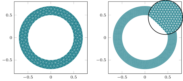
Figure 3. Triangulations of an annulus with an inner radius of 0.5 and outer radius of 0.7 for two different values of the mesh parameter $h$. Left: $h=0.05$, right: $h=0.01$.

Consider the obstacle $U=\overline{B_{1/2}(0)}\subset\mathbb{R}^{2}$, i.e. the disk of radius $\frac{1}{2}$. We chose $X=1$ and used the meshing tool Distmesh [24] to compute triangulations of the annulus $B_{X}\setminus U$ for the seven values $h\in\{0.08,0.05,0.02,0.01,0.005,0.002,0.001\}$ of the meshing parameter (cf. Figure 3 for two examples).

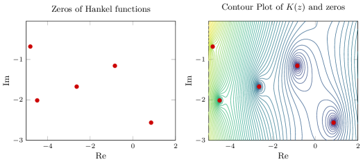
Figure 4. Resonances of $U$ in the complex plane. Left: Computed directly from Hankel functions with high accuracy. Right: Contour plot of $\log|\det(T_{n}(k))|$, computed as described in Section LABEL:, together with its zeros (red dots). The reference point

Figure 4 (right) shows a contour plot of $T_{n}(k)$ for $N=6$ and $J=100$.

6.1.1. Details of the implementation

Even though the relationship $Nh^{\frac{4}{5}}\to 0$ theoretically guarantees convergence, the relative constant between $N$ and $h$ is important and unknown in practice. We therefore use the following heuristic to choose an optimal value of $N$ for any given (finite) $h$:

1. Compute the matrix $T_{n}(k)$ for a large value of $N$,

2. Consider its diagonal elements (see Figure 5). By compactness they should tend to 0 at the ends. However, for large $N$ an aliasing-type phenomenon takes over and after reaching a minimum they start growing.

3. Decrease $N$ until the minimum of $|\operatorname{diag}(T_{n}(k))|$ is reached at the ends of the matrix.

For the disk obstacle, this process yielded the values in Table 1.

$h$	0.08	0.05	0.02	0.01	0.005	0.002	0.001
$N$	6	7	10	13	17	28	39

Table 1. Optimal values of $N$ for different values of $h$.

This relationship is approximately quadratic, i.e. $N\sim h^{-\frac{1}{2}}$, as the right hand plot in Figure 5 shows: plotting $N^{2}$ against $h^{-1}$ gives an approximately straight line.

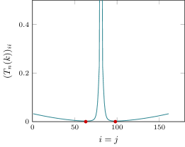
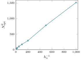
Figure 5. Left: diagonal elements of $|T_{n}|$ for $h=0.08$, $N=6$. The red dots mark its minima, which we interpret as the optimal size of the matrix $T_{n}$. Right: square of optimal value of $N$ (determined as in Section 6.1.1), plotted against $h^{-1}$.

6.1.2. Convergence analysis

In order to test the convergence rate as $h^{-1}$, $N\to\infty$ we chose the resonance near $-0.84-1.15\mathrm{i}$ (the second from the right in Figure 4) and increase $h^{-1}$, $N$ according to Table 1. We shall henceforth refer to the exact value of the resonance as $k_{\text{exact}}$. A zero finding procedure on $H^{(1)}_{0}$ yields the first 16 digits of $k_{\text{exact}}$ as

$$k_{\text{exact}}=-0.838549208188362-1.154799048234411\mathrm{i}+O(10^{-17}).$$

Due to natural limits in memory and computation time, the number $J$ of eigenfunctions in the Aitken’s corrector was kept fixed at $J=100$. In order to ensure the Aitken’s error remains negligible nevertheless, we adhered to the following process:

1. Choose a reasonable value for $k_{0}$ by inspecting Figure 4, say $k_{0}=-1-1\mathrm{i}$. Compute a first approximation $\gamma$ of $k_{\text{exact}}$ by minimising $\left|\det(T_{n}(k))\right|$ (we performed gradient descent until $\left|\det(T_{n}(k))\right|<10^{-16}$).

2. Set $k_{0}:=\gamma$ and recompute the approximation. Call it $\gamma_{h}$.

3. Set $k_{0}:=\gamma_{h}$, increase $h^{-1}$, $N$ and recompute the approximation $\gamma_{h}$.

4. Set $k_{0}:=\gamma_{h}$ and proceed in this fashion.

This process ensures that $|k_{0}-k|$ remains small for any $k$ that is used in the computation. As a consequence, the Atkinson error remains negligible even for modest values of $J$.

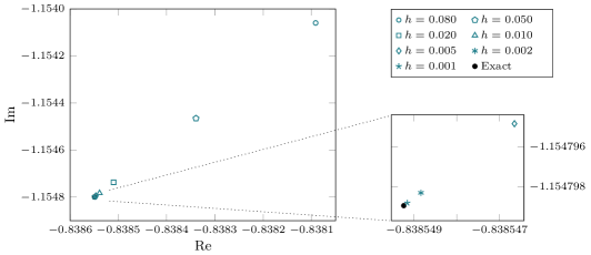
Figure 6. Convergence of successive approximations of $k_{\text{exact}}$ in the complex plane.

The results of this approximation procedure are shown in Figures 6 and 7. As the plots suggest, the approximation error converges to 0 as $h\to 0$. The slope of the line in Figure 7 suggests a convergence rate of $|k_{\text{exact}}-\gamma_{h}|\sim h^{2}$, in accordance with the FEM error of a domain with smooth boundary.

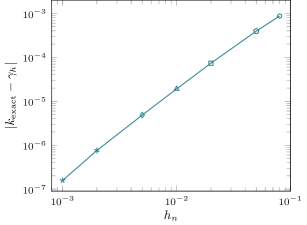
Figure 7. Approximation error $|k_{\text{exact}}-\gamma_{h}|$ for $h$ in Table 1.

6.2. A filled Julia set

Next we demonstrate the algorithm’s capabilities on domains with fractal boundary. We compute the resonances on a sequence of Julia sets depending on a parameter $q\in[0,0.733]$, which morph from a disk for $q=0$ into an irregular set (cf. Figure 8).

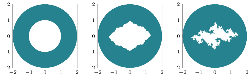
Figure 8. Examples of the Julia sets used in the computation. Left: $q=0$, centre: $q=0.4$, right: $q=0.733$.

For any complex number $c$ the filled Julia set $\mathcal{J}_{c}$ is defined by

(6.1) $$\mathcal{J}_{c}=\{z\in\mathbb{C}\,|\,f^{\circ k}(z)\text{ bounded as }k\to\infty\},$$

where $f(z)=z^{2}+c$ and $f^{\circ k}$ denote the $k$th iterate of $f$. It can be shown [12] that $J_{c}$ has an interior if and only if $c$ is in the Mandelbrot set. For our numerical experiment we choose $c=q(-1+0.2\mathrm{i}),$ where $q$ varies from 0 to $0.7$ in steps of $0.05$. If $q=0.75$, then $c$ is outside the Mandlbrot set and $J_{c}$ fails to satisfy Assumption 2.9. In order to capture the behaviour of the resonances at the boundary we added the values $q\in\{0.71,0.72,0.73,0.733\}$ yielding 19 resonance computations in total.

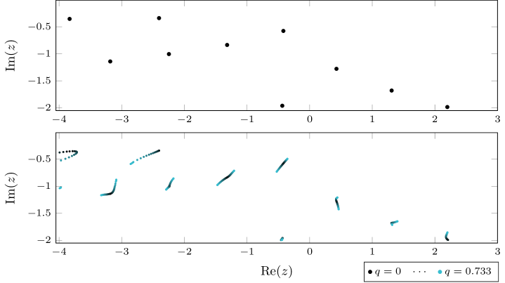
Figure 9. Movement of resonances in the complex plane as $q$ varies from 0 to $0.733$. Top: computed resonances for $q=0$ (the disk obstacle). Bottom: paths traced out by the resonances. Cyan intensity corresponds to larger $q$.

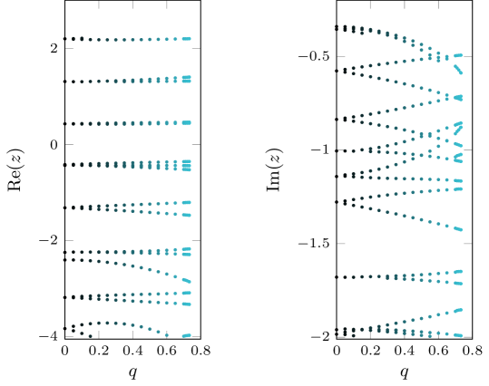
Figure 10. Real and imaginary parts of the computed resonances as a function of $q$. Left: real part, right: imaginary part.

Remark 6.1 (Mesh generation).

The mesh generation for the filled Julia set was done with a combination of Distmesh (for the outer part) and a pixelation method similar to [26]. Pixels were added to the mesh if their midpoint was determined to lie outside the filled Julia set, as determined numerically by truncating the iteration in (6.1). The pixel size in Figure 8 corresponds to the pixel size in our meshing.

Figures 9 and 10 show the results of our algorithm for this sequence of sets. For $q=0$ the computation yields the familiar resonances of a disk obstacle (Figure 9 (top) is a scaled version of Figure 4). As $q$ increases, the resonances begin to split and drift apart. This is in accordance with the geometry of the associated Julia sets: The disk-shaped domain for $q=0$ is rotationally symmetric. This symmetry is broken more and more as $q$ increases, as Figure 8 illustrates. As a result the resonances become less and less degenerated. An animation of the full sequence is available at frank-roesler.github.io/images/research/rough_reson_anim.gif.

6.3. The Koch Snowflake

Finally, we consider the Koch Snowflake, which also satisfies Assumption 2.9. A natural sequence $U_{n}$ with the appropriate convergence properties is given by the Koch prefractals, which can be easily computed and triangulated. In this section we use our algorithm to explore how resonances change as the prefractals approximate the Koch Snowflake.

Figure 11. Meshes for both the 2nd (left) and the 5th (right) iteration of the Koch Snowflake used in our computation.

We computed triangulated domains for the Koch iterations 2, 3, 4 and 5, cf. Figure 11 for illustrations of the 2nd and 5th iterations. Figure 13 shows example visualisations of the results for the third Koch iteration for two regions in the complex plane (near $-1$ and $-14$, respectively). The algorithm yields three resonances near $-14$ and one resonance near $-1$.

Figure 12. Resonances and contour plots of $\log|\det(T_{n}(k))|$ for the third iteration of the Koch Snowflake near $k_{0}=-1-1i$ and $k_{0}=-14-1i$.

As the Koch iteration increases and the boundary of the prefractals becomes more and more irregular as they approximate the Koch curve. In this process, more and more small cavities open up in the boundary and one would expect waves of appropriate wave lengths to become increasingly trapped. As a consequence, we would expect the higher resonances (whose wavelength fits the cavities) to depend more strongly on the Koch iteration than the lower ones (whose wave length corresponds to the large scale structure of the domain).

This intuitive understanding is supported by our numerical results, as is shown in Figure 13. As the Koch iteration increases from 2 to 5, the three resonances near $-14$ move to the right in steps of order $10^{-1}$. The resonances near $-1$, on the other hand, move by an order of magnitude less, with steps of order $10^{-2}$.

Figure 13. Movement of resonances as the Koch iteration increases. Brighter cyan colours correspond to larger Koch iteration.

Appendix A Scattering resonances with NtD operators

Recall the definition of the solution operator $S(k)$ (4.2). Consider the annulus

$$A_{X}=B_{X}(0)\backslash\overline{B_{X-1}(0)}.$$

Denote the inner boundary of $A_{X}$ by

$$\Gamma_{X-1}:=\partial B_{X-1}(0).$$

Let

$$S^{A}\in\mathcal{B}(H^{-\frac{1}{2}}(\Gamma);H^{1}(A_{X}))$$

denote the solution operator for the BVP

(A.1) $$\begin{cases}-\Delta u=0\quad\text{on}\quad A_{X}\quad\\ \partial_{\nu}|_{\Gamma}u=g,\quad\partial_{\nu}|_{\Gamma_{X-1}}u=-\frac{X}{X-1}g\end{cases}.$$

Note that the above boundary value problems are well-posed since the compatibility condition

(A.2) $$\int_{\partial A}\partial_{\nu}|_{\partial A}u=0.$$

Next, let $R(k):=(-\Delta_{\mathrm{ND}}^{\Omega}-k^{2})^{-1}$, $k\in\mathbb{C}_{+}$, denote the resolvent operator for the Laplacian $-\Delta_{\mathrm{ND}}^{\Omega}$ on $L^{2}(\Omega)$ endowed Dirichlet boundary conditions on $\partial U$ and Neumann boundary conditions on $\Gamma$. Finally, we introduce a smooth cutoff function $\chi\in C^{\infty}(A_{X})$ such that

$$\chi=\begin{cases}1\quad\text{near}\quad\Gamma\\ 0\quad\text{near}\quad\Gamma_{X-1}\end{cases}.$$

Lemma A.1.

The operator $S(k)$ admits the decomposition

(A.3) $$S(k)=\chi S^{A}+R(k)D_{\chi}(k)S^{A},\qquad k\in\mathbb{C}_{+},$$

where, $D_{\chi}(k)\in\mathcal{B}(H^{1}(A_{X});L^{2}(\Omega))$ is a first order differential operator defined by

(A.4) $$D_{\chi}(k)=k^{2}\chi+\Delta(\chi)+2\nabla(\chi)\cdot\nabla,\qquad k\in\mathbb{C}_{-}.$$

Proof.

For arbitrary $g\in H^{-1/2}(\Gamma)$, let $u=S(k)g$ and $v=S^{A}g$. Consider the function $w:=u-\chi v$. We aim to show that $w=R(k)D_{\chi}(k)v$. Keeping in mind that $u$ and $v$ are smooth functions by interior elliptic regularity, we compute,

$$-\Delta w =-\Delta u+\Delta(\chi)v+2\nabla(\chi)\cdot\nabla(v)+\chi\Delta(v)$$

$$=k^{2}(u-\chi v)+k^{2}\chi v+\Delta(\chi)v+2\nabla(\chi)\cdot\nabla(v)$$

$$=k^{2}w+D_{\chi}(k)v.$$

Since $u\in H^{1}_{\mathrm{ND}}(\Omega)$ and $v\in H^{1}(A_{X})$, an extension by zero shows that $w=u-\chi v\in H^{1}_{\mathrm{ND}}(\Omega)$, completing the proof. ∎

Lemma A.2.

There exist a compact operator $K^{A}$ such that

$$\mathcal{N}^{1/2}\gamma_{\Gamma}S^{A}\mathcal{N}^{1/2}=X+K^{A}.$$

Furthermore, for any $s\in\mathbb{R}$, the operators $\mathcal{N}^{s}K^{A}$ and $K^{A}\mathcal{N}^{s}$ are also compact and $S^{A}:H^{\frac{1}{2}}(\Gamma)\to H^{1}(A_{X})$ is bounded.

Proof.

The result follows from the matrix representation of $S^{A}$ in the basis $\{e_{\alpha}\}_{\alpha\in\mathbb{Z}}$, which we will derive by explicit calculation. For $\alpha\in\mathbb{Z}$ let $u=S^{A}e_{\alpha}$. A separation ansatz in polar coordinates $u(r,\theta)=\rho(r)\phi(\theta)$ gives the general solution

(A.5) $$\rho(r)=c_{1}r^{\alpha}+c_{2}r^{-\alpha}\qquad\text{and}\qquad\phi(\theta)=e_{\alpha}(\theta),$$

with $c_{1}$, $c_{2}$ to be determined. Imposing the boundary conditions $\partial_{\nu}|_{\Gamma}u=e_{\alpha}$, $\partial_{\nu}|_{\Gamma^{\prime}}u=-\frac{X}{X-1}e_{\alpha}$ and a direct calculation yields

(A.6) $$c_{1}=\frac{X}{\alpha}\frac{1}{X^{\alpha}-(X-1)^{\alpha}}\qquad\text{and}\qquad c_{2}=\frac{X}{\alpha}\frac{1}{(X-1)^{-\alpha}-X^{-\alpha}}$$

and thus

(A.7) $$\rho(r)=\frac{X}{\alpha}\left(\frac{r^{\alpha}}{X^{\alpha}-(X-1)^{\alpha}}+\frac{r^{-\alpha}}{(X-1)^{-\alpha}-X^{-\alpha}}\right)$$

From (A.7) we immediately conclude that

$$\gamma_{\Gamma}S^{A}(e_{\alpha})=\frac{X}{\alpha}\left(\frac{X^{\alpha}+(X-1)^{\alpha}}{X^{\alpha}-(X-1)^{\alpha}}\right)e_{\alpha}(\theta).$$

Hence $\gamma_{\Gamma}S^{A}$ is diagonal in the basis $\{e_{\alpha}\}_{\alpha\in\mathbb{Z}}$. We conclude that for any $\alpha\neq 0$

(A.8) $$\bigl{(}\mathcal{N}^{\frac{1}{2}}\gamma_{\Gamma}S^{A}\mathcal{N}^{\frac{1}{2}}\bigr{)}_{\alpha\alpha} =X\frac{|\alpha|}{\alpha}\frac{X^{\alpha}+(X-1)^{\alpha}}{X^{\alpha}-(X-1)^{\alpha}}$$

(A.9) $$=\begin{cases}X+2X\left(\bigl{(}\frac{X}{X-1}\bigr{)}^{\alpha}-1\right)^{-1}&\text{for }\alpha>0\\[5.69054pt] X-2X\left(1-\left(\frac{X-1}{X}\right)^{\alpha}\right)^{-1}&\text{for }\alpha<0\end{cases}$$

Since the terms $((X/(X-1))^{\alpha}-1)^{-1}$ and $((X-1)/X)^{\alpha}-1)^{-1}$ decay exponentially as $\alpha\to+\infty,-\infty$, respectively, eq. (A.8) immediately implies the assertion.

To prove boundedness of $S^{A}:H^{\frac{1}{2}}(\Gamma)\to H^{1}(A_{X})$, consider $u_{\alpha}:=S^{A}(\alpha^{-\frac{1}{2}}e_{\alpha})$. The above calculation yields

$$u_{\alpha}(r,\theta)=\alpha^{-\frac{1}{2}}\rho(r)e_{\alpha}(\theta).$$

A lengthy calculation yields explicit formulas for $\|u_{\alpha}\|_{L^{2}}$, $\|u_{\alpha}^{\prime}\|_{L^{2}}$, which imply

(A.10) $$\|u_{\alpha}\|_{L^{2}} \sim\alpha^{-1}\quad\text{ as }\alpha\to\pm\infty$$

(A.11) $$\|u_{\alpha}^{\prime}\|_{L^{2}} \sim 1\quad\text{ as }\alpha\to\pm\infty,$$

which immediately implies the desired $H^{1}$-boundedness. ∎

Lemma A.3.

There exists an analytic family of compact operators $K(k)$, $k\in\mathbb{C}_{-}$, on $L^{2}(\Gamma)$ such that

$$\frac{1}{2}\mathcal{N}^{\frac{1}{2}}(N_{1}(k)+M_{\mathrm{in}}(k)N_{2}(k))\mathcal{N}^{-\frac{1}{2}}=I+K(k),\qquad k\in\mathbb{C}_{-}.$$

Furthermore, $K(k)$ is bounded on $L^{2}(\Gamma)$ locally uniformly for $k\in\mathbb{C}_{-}$.

Proof.

Let $k\in\mathbb{C}_{-}$. Recalling the definitions of $N_{1}$ and $N_{2}$ we have

$$N_{1}(k)_{\alpha\alpha}:=\frac{H^{(1)}_{|\alpha|}(kX)}{A_{|\alpha|}(k)},\qquad N_{2}(k)_{\alpha\alpha}:=\frac{(H_{|\alpha|}^{(1)})^{\prime}(kX)}{A_{|\alpha|}(k)}$$

and $N_{i}(k)_{\alpha\beta}=0$ otherwise, where $A_{\nu}:=-i\sqrt{\frac{2}{\pi\nu}}\left(\frac{ekX}{2\nu}\right)^{-\nu}$. By well-known properties for Bessel functions (cf. (2.9)) we have

(A.12) $$\lim_{|\alpha|\to\infty}N_{1}(k)_{\alpha\alpha} =1$$

and hence

(A.13) $$N_{1}(k)=I+K_{1}(k),$$

where $K_{1}(k)=\operatorname{diag}\left(\frac{H^{(1)}_{|\alpha|}(kX)}{A_{|\alpha|}(k)}-1,\alpha\in\mathbb{Z}\right)$ is compact. Similarly, for $N_{2}$ we have

(A.14) $$N_{2}(k)_{\alpha\alpha} =A_{|\alpha|}(k)^{-1}\bigg{(}kH_{|\alpha|-1}^{(1)}(kX)-\frac{|\alpha|}{X}H_{|\alpha|}^{(1)}(kX)\bigg{)},$$

where we have used the general formula $\frac{d}{dz}H^{(1)}_{\nu}(z)=H_{\nu-1}^{(1)}(z)-\frac{\nu}{z}H_{\nu}^{(1)}(z)$. The first term on the right-hand side of (A.14) behaves like

$$\frac{kH_{|\alpha|-1}^{(1)}(kX)}{A_{|\alpha|}(k)} \sim c\frac{(|\alpha|-1)^{|\alpha|-1}}{|\alpha|^{|\alpha|}}$$

$$\xrightarrow{|\alpha|\to\infty}0$$

for a suitable constant $c$. Hence, comparing to (A.14) we obtain

(A.15) $$N_{2}(k) =-X^{-1}\mathcal{N}+K_{2}(k),$$

where $K_{2}(k)=\operatorname{diag}\left(\frac{kH_{|\alpha|-1}^{(1)}(kX)}{A_{|\alpha|}(k)},\alpha\in\mathbb{Z}\right)$ is compact. Collecting results, we have shown

(A.16) $$\mathcal{N}^{\frac{1}{2}}N_{1}(k)\mathcal{N}^{-\frac{1}{2}} =I+K_{1}(k)$$

(A.17) $$N_{2}(k)\mathcal{N}^{-\frac{1}{2}} =-X^{-1}\mathcal{N}^{\frac{1}{2}}+\mathcal{N}^{-\frac{1}{2}}K_{2}(k).$$

It remains to control $M_{\mathrm{in}}(k)$. Combining Lemmas A.1 and A.2 we have

$$M_{\mathrm{in}}(k) =\gamma_{\Gamma}S(k)$$

$$=\gamma_{\Gamma}(\chi S^{A}+R(k)D_{\chi}(k)S^{A})$$

and

$$\mathcal{N}^{\frac{1}{2}}M_{\mathrm{in}}(k)\mathcal{N}^{\frac{1}{2}} =\mathcal{N}^{\frac{1}{2}}\gamma_{\Gamma}\chi S^{A}\mathcal{N}^{\frac{1}{2}}+\mathcal{N}^{\frac{1}{2}}\gamma_{\Gamma}R(k)D_{\chi}(k)S^{A}\mathcal{N}^{\frac{1}{2}}$$

$$=\mathcal{N}^{\frac{1}{2}}\gamma_{\Gamma}S^{A}\mathcal{N}^{\frac{1}{2}}+\mathcal{N}^{\frac{1}{2}}\gamma_{\Gamma}R(k)D_{\chi}(k)S^{A}\mathcal{N}^{\frac{1}{2}}$$

$$=X+K^{A}+\mathcal{N}^{\frac{1}{2}}\gamma_{\Gamma}R(k)D_{\chi}(k)S^{A}\mathcal{N}^{\frac{1}{2}}.$$

We simplify notation by writing

(A.18) $$\mathcal{N}^{\frac{1}{2}}M_{\mathrm{in}}(k)\mathcal{N}^{\frac{1}{2}}=X+K_{3}(k),$$

where $K_{3}(k)=K^{A}+\mathcal{N}^{\frac{1}{2}}\gamma_{\Gamma}R(k)D_{\chi}(k)S^{A}\mathcal{N}^{\frac{1}{2}}$. Combining (A.18) and (A.17) we obtain

$$\mathcal{N}^{\frac{1}{2}}M_{\mathrm{in}}(k)N_{2}(k)\mathcal{N}^{-\frac{1}{2}} =\mathcal{N}^{\frac{1}{2}}M_{\mathrm{in}}(k)(-X^{-1}\mathcal{N}^{\frac{1}{2}}+\mathcal{N}^{-\frac{1}{2}}K_{2}(k))$$

$$=-X^{-1}\mathcal{N}^{\frac{1}{2}}M_{\mathrm{in}}(k)\mathcal{N}^{\frac{1}{2}}+\mathcal{N}^{\frac{1}{2}}M_{\mathrm{in}}(k)\mathcal{N}^{-\frac{1}{2}}K_{2}(k)$$

$$=\mathcal{N}^{\frac{1}{2}}M_{\mathrm{in}}(k)\mathcal{N}^{\frac{1}{2}}(-X^{-1}+\mathcal{N}^{-1}K_{2}(k))$$

$$=(X+K_{3}(k))(-X^{-1}+\mathcal{N}^{-1}K_{2}(k))$$

(A.19) $$=I-X^{-1}K_{3}(k)+X\mathcal{N}^{-1}K_{2}(k)+K_{3}(k)\mathcal{N}^{-1}K_{2}(k)$$

Combining (A.19) and (A.16) we obtain the final formula

(A.20) $$\frac{1}{2}\mathcal{N}^{\frac{1}{2}}(N_{1}(k)+M_{\mathrm{in}}(k)N_{2}(k))\mathcal{N}^{-\frac{1}{2}} =I+K(k),$$

where

(A.21) $$2K(k)=K_{1}(k)-X^{-1}K_{3}(k)+X\mathcal{N}^{-1}K_{2}(k)+K_{3}(k)\mathcal{N}^{-1}K_{2}(k).$$

To prove the assertion, it remains to show that $K(k)$ is compact for every $k\in\mathbb{C}_{-}$ and that $K(k)$ is locally uniformly bounded on $L^{2}(\Gamma)$.

Local uniform boundedness follows from continuity of $H_{\nu}^{(1)}$, $D_{\chi}$ in $\mathbb{C}_{-}$ and the fact that $A_{\nu}$ has no zeros in $\mathbb{C}_{-}$. To prove compactness we consider each term in (A.21) separately. Compactness of $K_{1}$ is already established, thus we focus on $K_{3}$. $K^{A}$ is compact by Lemma A.2, so it suffices to prove compactness of $\mathcal{N}^{\frac{1}{2}}\gamma_{\Gamma}R(k)D_{\chi}(k)S^{A}\mathcal{N}^{\frac{1}{2}}$. Employing Lemmas A.1, A.2 we have the following sequence of bounded operators

$$L^{2}(\Gamma)\xrightarrow{\mathcal{N}^{\frac{1}{2}}}H^{\frac{1}{2}}(\Gamma)\xrightarrow{S^{A}}H^{1}(A_{X})\xrightarrow{D_{\chi}(k)}L^{2}(\Omega)\xrightarrow{\chi R(k)}H^{2}(\Omega)\xrightarrow{\gamma_{\Gamma}}H^{\frac{3}{2}}(\Gamma)\xrightarrow{\mathcal{N}^{\frac{1}{2}}}H^{1}(\Gamma),$$

where we have used the fact that $\gamma_{\Gamma}\chi R(k)=\gamma_{\Gamma}R(k)$. We conclude that the range of $\mathcal{N}^{\frac{1}{2}}\gamma_{\Gamma}R(k)D_{\chi}(k)S^{A}\mathcal{N}^{\frac{1}{2}}$ is compactly embedded in $L^{2}(\Gamma)$, proving compactness of the operator and of $K_{3}(k)$.

It only remains to prove compactness of $\mathcal{N}^{-1}K_{2}(k)$. However, this is trivial, since $K_{2}(k)$ is bounded and $\mathcal{N}^{-1}$ is compact. ∎

References

- [1] H. Ammari, H. Kang, and H. Lee. Layer potential techniques in spectral analysis. Number 153. American Mathematical Soc., 2009.
- [2] J. Ben-Artzi, M. J. Colbrook, A. C. Hansen, O. Nevanlinna, and M. Seidel. Computing Spectra–On the Solvability Complexity Index Hierarchy and Towers of Algorithms. arXiv:1508.03280, 2020.
- [3] J. Ben-Artzi, A. C. Hansen, O. Nevanlinna, and M. Seidel. New barriers in complexity theory: on the solvability complexity index and the towers of algorithms. C. R. Math. Acad. Sci. Paris, 353(10):931–936, 2015.
- [4] J. Ben-Artzi, M. Marletta, and F. Rösler. Computing the sound of the sea in a seashell. Found. Comput. Math., 22(3):697–731, 2022.
- [5] J. Ben-Artzi, M. Marletta, and F. Rösler. Computing scattering resonances. J. Eur. Math. Soc. (JEMS), 25(9):3633–3663, 2023.
- [6] H. Brezis and P. Mironescu. Gagliardo-Nirenberg inequalities and non-inequalities: the full story. Ann. Inst. H. Poincaré C Anal. Non Linéaire, 35(5):1355–1376, 2018.
- [7] S. N. Chandler-Wilde, D. P. Hewett, A. Moiola, and J. Besson. Boundary element methods for acoustic scattering by fractal screens. Numer. Math., 147(4):785–837, 2021.
- [8] M. J. Colbrook. On the computation of geometric features of spectra of linear operators on Hilbert spaces. Foundations of Computational Mathematics, 2019.
- [9] M. J. Colbrook and A. C. Hansen. The foundations of spectral computations via the solvability complexity index hierarchy. J. Eur. Math. Soc. (JEMS), 25(12):4639–4718, 2023.
- [10] NIST Digital Library of Mathematical Functions. https://dlmf.nist.gov/, Release 1.1.12 of 2023-12-15. F. W. J. Olver, A. B. Olde Daalhuis, D. W. Lozier, B. I. Schneider, R. F. Boisvert, C. W. Clark, B. R. Miller, B. V. Saunders, H. S. Cohl, and M. A. McClain, eds.
- [11] S. Dyatlov and M. Zworski. Mathematical theory of scattering resonances, volume 200 of Graduate Studies in Mathematics. American Mathematical Society, Providence, RI, 2019.
- [12] K. Falconer. Fractal Geometry: Mathematical Foundations and Applications. John Wiley & Sons, 2004.
- [13] J. Fleckinger and D. G. Vassiliev. An Example of a Two-Term Asymptotics for the “Counting Function” of a Fractal Drum. Transactions of the American Mathematical Society, 337(1):99–116, 1993.
- [14] S. Félix, B. Sapoval, M. Filoche, and M. Asch. Enhanced wave absorption through irregular interfaces. Europhysics Letters, 85(1):14003, jan 2009.
- [15] A. C. Hansen. On the Solvability Complexity Index, the n-pseudospectrum and approximations of spectra of operators. Journal of the American Mathematical Society, 24(1):81–81, 2011.
- [16] M. Hinz, A. Rozanova-Pierrat, and A. Teplyaev. Non-Lipschitz uniform domain shape optimization in linear acoustics. SIAM Journal on Control and Optimization, 59(2):1007–1032, 2021.
- [17] C. Hua and B. D. Sleeman. Fractal drums and then-dimensional modified Weyl-Berry conjecture. Communications in Mathematical Physics, 168(3):581–607, 1995.
- [18] M. L. Lapidus. Fractal drum, inverse spectral problems for elliptic operators and a partial resolution of the Weyl-Berry conjecture. Transactions of the American Mathematical Society, 325(2):465–529, 1991.
- [19] M. L. Lapidus and C. Pomerance. Counterexamples to the modified Weyl-Berry conjecture on fractal drums. Math. Proc. Cambridge Philos. Soc., 119(1):167–178, 1996.
- [20] M. Levitin and M. Marletta. A simple method of calculating eigenvalues and resonances in domains with infinite regular ends. Proc. Roy. Soc. Edinburgh Sect. A, 138(5):1043–1065, 2008.
- [21] M. Levitin and A. Strohmaier. Computations of eigenvalues and resonances on perturbed hyperbolic surfaces with cusps. Int. Math. Res. Not. IMRN, (6):4003–4050, 2021.
- [22] M. Levitin and D. Vassiliev. Spectral Asymptotics, Renewal Theorem, and the Berry Conjecture for a Class of Fractals. Proceedings of the London Mathematical Society, s3-72(1):188–214, 1996.
- [23] W. C. H. McLean. Strongly elliptic systems and boundary integral equations. Cambridge university press, 2000.
- [24] P.-O. Persson and G. Strang. A simple mesh generator in matlab. SIAM review, 46(2):329–345, 2004.
- [25] G. Roddick. Computation of scattering matrices and their derivatives for waveguides. J. Comput. Appl. Math., 396:Paper No. 113453, 24, 2021.
- [26] F. Rösler and A. Stepanenko. Computing eigenvalues of the Laplacian on rough domains. Math. Comp., 93(345):111–161, 2023.
- [27] A. E. Taylor and D. C. Lay. Introduction to functional analysis, volume 1. Wiley New York, 1958.