When to Preempt in a Status Update System?

Abstract

We consider a time slotted status update system with an error-free preemptive queue. The goal of the sampler-scheduler pair is to minimize the age of information at the monitor by sampling and transmitting the freshly sampled update packets to the monitor. The sampler-scheduler pair also has a choice to preempt an old update packet from the server and transmit a new update packet to the server. We formulate this problem as a Markov decision process and find the optimal sampling policy. We show that it is optimal for the sampler-scheduler pair to sample a new packet immediately upon the reception of an update packet at the monitor. We also show that the optimal choice for the scheduler is to preempt an update packet in the server, if the age of that packet crosses a fixed threshold. Finally, we find the optimal preemption threshold when the range of the service time of the server is finite, otherwise we find the $\epsilon$-optimal preemption threshold.

I Introduction

We consider a network model which comprises a source, a sampler, a scheduler, a transmitter, a preemptive server and a monitor. The source is a stochastic process which the monitor aims to track in real-time. At a given time slot $t$, the sampler samples an update packet and aims that the monitor receives this update packet so that the monitor has a fresh information about the source. Let us consider that at time $t$, when the sampler samples a new update packet, the server is busy serving a previously sampled update packet. Then, the scheduler has to decide whether to preempt the old update packet and transmit the new update packet, or to keep transmitting the old update packet and discard the new update packet. The preemptive nature of the server considered in this paper gives an extra degrees of freedom to the scheduler to minimize the age of information compared to a non-preemptive server. A sampling algorithm $\pi$ is composed of a sampling policy of the sampler as well as a preemption policy of the scheduler. Our goal is to devise a sampling and preemption algorithm such that the monitor has as fresh information as possible about the source. We characterize this freshness by the well-studied metric of age of information [1, 2, 3]. Fig. 1 provides a pictorial representation of the considered network model.

The sampling problem in the context of age of information minimization has been studied in the literature, see e.g., [4, 5]. These works consider non-preemptive servers, i.e., a packet being served cannot be dropped from the server and the scheduler has to wait until the monitor receives the currently served packet. Due to that, these works can only optimize the initial sampling times. In contrast, in this paper, we can optimize the initial sampling times as well as the preemption times. Now, between two successful receptions of the update packets at the monitor, there can be multiple preemptions. Thus, in principle, in this paper, we have to deal with countably infinite optimization parameters, which makes the studied problem challenging.

The sampling problem to minimize the age of information with possible preemption has also been studied in the literature under different network settings, see e.g., [6, 7, 8]. Reference [6] considers a network model which is similar to our model, except that it is in continuous time whereas ours is in discrete time. To combat the countably infinite optimization parameters, [6] finds the optimal policy from the set of policies for which the preemption threshold is fixed and independent of the sample indices, i.e., if the service time of a packet in the server exceeds a fixed threshold then the scheduler-sampler pair drops the current packet and samples a fresh packet from the source and submits it to the server. Thus, [6] optimizes two parameters to find the optimal policy, the initial sampling time, i.e., when to sample an update packet when the server is empty, and the preemption threshold. In contrast, in this paper, we provide an optimal policy over the set of all causal policies for the discrete time setting.

In this paper, first, we formulate a Markov decision process (MDP) for the considered optimization problem. Then, we show that there exists a stationary sampling and preemption policy which is optimal for the considered problem. Then, we find several structural properties for the optimal policy for the MDP. Namely, we find that the zero-wait sampling policy is optimal and the preemption policy has a threshold structure which is independent of the age of the monitor and depends only on the age of the packet being served at the server. That is, the preemption threshold is constant and independent of the packet index. We finally, find the optimal preemption threshold for a bounded service time, otherwise we find the $\epsilon$-optimal preemption threshold.

II System Model and Problem Formulation

We consider a time slotted model, where a sampler can generate an update packet at any time slot it wishes, i.e., we consider a generate-at-will model. The sampler aims to minimize the age of a monitor by delivering the fresh update packets. We model the communication channel as an error-free preemptive queue. As we are interested in freshness, at time slot $t$, the sampler samples a new packet only if either the queue is empty or the sampler decides to preempt the existing packet in the queue [4]. We denote a sampling policy as $\pi$. We consider a set of causal policies, i.e., the policies which depend only on the past observations and decisions, denoted by $\Pi$. We denote the generation time of the $i$th update packet corresponding to a sampling policy $\pi$ as $S_{i}^{\pi}$ and the delivery time of the $i$th packet as $D_{i}^{\pi}$. If the $i$th packet is preempted by the server, then we define $D_{i}^{\pi}=\infty$. At time $t$, we define the age of information of the monitor corresponding to a sampling policy, $\pi$ as $v^{\pi}(t)=t-S^{\pi}_{i}$, where $i=\sup{\{j:D_{j}^{\pi}\leq t\}}$. Thus, a sampling policy $\pi$ is completely defined as $\pi=(S_{1}^{\pi},S_{2}^{\pi},\cdots)$, and we are interested in solving the following problem,

$$\inf_{\pi\in\Pi} \limsup_{T\rightarrow\infty}\frac{1}{T}\sum_{t=1}^{T}\mathbb{E}_{\pi}[v^{\pi}(t)|v^{\pi}(1)=v],$$ (1)

where $v$ is the initial age of the monitor irrespective of $\pi$.

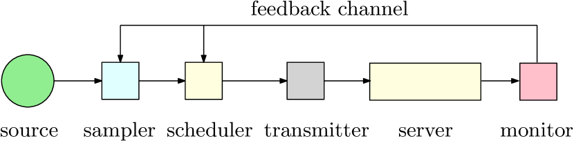
Figure 1: A sampler and a scheduler decide the packet flow through the server such that the monitor receives fresh information about the source.

Note that, it is not always guaranteed that the monitor will receive a certain sampled packet, as the sampler can preempt an update packet from the queue. When the monitor successfully receives an update packet for the $i$th time, we denote that event as $\mathcal{E}_{i}^{\pi}$, $i\in{\{0,1,2,\cdots\}}$. Without loss of generality, we assume that the event $\mathcal{E}_{0}^{\pi}$ occurs at time $t=0$. We denote the number of sampled update packets between the event $\mathcal{E}_{i}^{\pi}$ and $\mathcal{E}_{i+1}^{\pi}$ as $M_{i}^{\pi}$. Note that, $M_{i}^{\pi}=0$ implies that the sampler does not preempt any update packet after the $i$th sample packet received by the monitor until the $(i+1)$th sample packet is received by the monitor. We denote the time when the event $\mathcal{E}_{i}^{\pi}$ occurs with $\bar{D}_{i}^{\pi}$. We assume that $S_{0}^{\pi}=0$, irrespective of any policy $\pi$. The sample index of the update packet, upon the reception of which the event $\mathcal{E}_{i}$ occurs is,

$$k=\sum_{j=0}^{i-1}M_{j}^{\pi}+i.$$ (2)

We assume that the time taken to deliver the $k$th sampled packet, defined in (2), to the monitor is $Y_{i}$. We call $Y_{i}$ as the service time of the queue. We assume that the service time is independent and identically distributed over the index of the delivered sample $i$. Thus, for notational convenience, we use $Y$ as the service time. Note that the delivery time of a sampled packet to the monitor is independent of the policy and only depends on the statistics of the queue. Thus, the time when the event $\mathcal{E}_{i}$ occurs is $(S_{k}^{\pi}+Y_{i})$. We assume that $\mathbb{E}[Y_{i}]<\infty$. Now, we define the following quantities to solve (1). We define the first sampling time after the occurrence of the event $\mathcal{E}_{i}$ as $X_{i}^{\pi}$. Note that, there are $M^{\pi}_{i}$ numbers of samples between the event $\mathcal{E}_{i}$ and $\mathcal{E}_{i+1}$. Thus, using (2),

$$X_{i}^{\pi}=S_{k+1}^{\pi}-S_{k}^{\pi}.$$ (3)

Moreover, we denote the time interval between the $j$th sample and the $(j+1)$th sample in between the events $\mathcal{E}_{i+1}^{\pi}$ and $\mathcal{E}_{i}^{\pi}$, with $Z_{j,i}^{\pi}$, for $j\in{1,2,\cdots,(M_{i}^{\pi}-1)}$. From [4], we know that it is not optimal to sample a packet when the queue is busy, thus we assume that the waiting time for an update packet to get served by the queue is $0$. In other words, the sampler decides to sample an update packet only after a successful transmission of the serving packet in the queue, or if the sampler decides to preempt the serving packet in the queue. Thus, we can represent a scheduling algorithm as,

$$\pi=(X_{0}^{\pi},Z_{1,0}^{\pi},\cdots,Z_{M_{0}^{\pi}-1,0}^{\pi},X_{1}^{\pi},\cdots)$$ (4)

Due to the space limitations here, we provide proofs for some selective theorems, rest of the proofs will be provided in the journal version which will be posted on arXiv.

III Optimal Scheduling Algorithm

In this paper, we assume that whenever the scheduler preempts an update packet from the server, the scheduler-sampler pair immediately samples a new update packet from the source and decides to transmit this packet to the monitor. In the next theorem, we show that this is indeed the optimal thing to do. In other words, it is not optimal to wait for some time to sample a new packet when the scheduler preempts an update packet from the server.

Theorem 1.

It is always optimal for the scheduler-sampler pair to sample a new update packet from the source and transmit the packet to the monitor immediately after the scheduler decides to preempt a currently serving update packet.

Before formulating the problem in (1) in a Markov decision process (MDP), we define the components of the MDP.

State: We define a state of the system as a two dimensional vector $s=(v_{1},v_{2})$ where $v_{1}$ is the age of the monitor and $v_{2}$ is the age of the packet in the server. Similarly, we define the state of the system at time $t$ as $s(t)=(v_{1}(t),v_{2}(t))$. We define the set of all the states $s$ as the state space of the problem $\mathcal{S}$. Note that, $\mathcal{S}$ is a countably infinite set. If the server is empty and the age of the monitor is $v_{1}$, we represent the state of the system with $(v_{1},\infty)$. Note that, the age of the monitor can never be less than the age of the packet in the queue. Thus, we always assume that $s=(v_{1},v_{2})$, such that $v_{1}\geq v_{2}$. If with probability $1$, the service time $Y$ is finite, in other words, if there exists a finite positive integer $k$, such that the random variable is bounded by $k$, i.e.,

$$k=\inf\bigg{\{}\ell:\Big{(}\sum_{i=1}^{\ell}\mathbb{P}(Y=i)\Big{)}=1\bigg{\}}$$ (5)

then the age of the packet in the queue can never be greater than $k$. Thus, we modify the state space as

$$\!\mathcal{S}\!=\!\{(v_{1},v_{2})\!\cup\!(v_{1},\infty):v_{1}\geq v_{2},(v_{1},v_{2})\in{\mathbb{N}^{2}},v_{2}\leq k\}$$ (6)

where $\mathbb{P}(e)$ is the probability measure of event $e$.

Action: At time slot $t$, the sampler-scheduler pair has three actions to choose from. We write the action at time $t$ as $a(t)\in\{0,1,2\}$. Here, $a(t)=0$ means that at time $t$, the server is empty and the sampler does not sample a new update packet; $a(t)=1$ means that at time $t$, the sampler samples a fresh update packet and the scheduler decides to transmit it to the monitor, i.e., if at time slot $t$ the server is empty then the transmitter submits this packet to the server, or if the server is busy with serving a staler packet then the scheduler preempts that old update packet and submits the fresh update packet to the server; and $a(t)=2$ means that at time $t$ the server is serving an update packet and the scheduler decides to re-transmit that update packet.

Transition Probabilities: If the system is in state $s$ and the sampler-scheduler pair decides to choose an action $a$, then we denote the probability with which the system goes to the state $s^{\prime}\in{\mathcal{S}}$ as $P_{a}(s,s^{\prime})$. The transition probabilities depend on the statistics of the service time $Y$.

Cost: If the state of the system is $s\in{\mathcal{S}}$, and if the sampler-scheduler takes an action $a\in{\{0,1,2\}}$, then we define the cost incurred by the system as $C(s,a)=v_{1}$.

Thus, (1) can be reformulated as,

$$\inf_{\pi\in{\Pi}} \limsup_{T\rightarrow\infty}\frac{1}{T}\sum_{t=1}^{T}\mathbb{E}_{\pi}[C(s(t),a(t))|s(1)=(v,\infty)].$$ (7)

In (7) we assume that the initial age of the system is $v$ which is independent of the policy, and initially the queue is empty.

In the next theorem, we show that there exists a stationary policy which optimally solves the problem in (7).

Theorem 2.

There exists a stationary policy which is optimal for the following problem,

$$\inf_{\pi\in{\Pi}}\limsup_{T\rightarrow\infty}\frac{1}{T}\sum_{t=1}^{T}\mathbb{E}_{\pi}[C(s(t),a(t))|s(1)=(v,\infty)].$$ (8)

Next, we introduce the discounted MDP, which is well-known in the literature [9, 10], to prove the structural properties of an optimal solution for (7). For $0<\alpha<1$, we define the $\alpha$ discounted cost for an initial state $s$, corresponding to a policy $\pi$ as,

$$V_{\alpha}^{\pi}(s)=\sum_{t=1}^{\infty}\alpha^{T}\mathbb{E}_{\pi}[C(s(t),a(t))|s(0)=s].$$ (9)

We define the optimal discounted cost as, $V_{\alpha}(s)=\inf_{\pi\in{\Pi}}V_{\alpha}^{\pi}$. We define the following quantity which will be useful for future presentation,

$$V_{\alpha}(s;a)=C(s,a)+\alpha\sum_{\tilde{s}\in{\mathcal{S}}}P_{a}(s,\tilde{s})V_{\alpha}(\tilde{s}).$$ (10)

Next, we state a lemma regarding the discounted cost MDP, which is well-known in the literature [9, 10].

Lemma 1.

For every state $s\in{\mathcal{S}}$ and $0<\alpha<1$, if $V_{\alpha}(s)$ is finite, then $V_{\alpha}(s)$ satisfies the following equation,

$$V_{\alpha}(s)=\min_{a\in{\{0,1,2\}}}V_{\alpha}(s;a).$$ (11)

For all states $s\in{\mathcal{S}}$ and $0<\alpha<1$, we define $V_{\alpha,0}(s)=0$ and for $n\geq 1$,

$$\!\!V_{\alpha,n}(s)\!=\!\max_{a\in{\{0,1,2\}}}\{C(s,a)+\alpha\sum_{\tilde{s}\in{\mathcal{S}}}P_{a}(s,\tilde{s})V_{\alpha,n-1}(\tilde{s})\}.\!$$ (12)

From [9, 10], we know

$$\lim_{n\rightarrow\infty}V_{\alpha,n}(s)=V_{\alpha}(s).$$ (13)

Now, to prove the crucial results in this paper, we consider a continuous state space $\bar{\mathcal{S}}$, where a state $s\in{\bar{\mathcal{S}}}$, has the same structure as a state $s^{\prime}\in{\mathcal{S}}$, however the components of $s$ can take values from the set of real numbers. We consider an MDP on the state space $\bar{\mathcal{S}}$. The cost and action spaces of this new MDP are the same as the original MDP. We keep the structure of the transition probabilities for this new MDP the same as the original MDP. Namely, from a state $s=(v_{1},v_{2})$, the transition can happen only to a state $s^{\prime}=(v_{1}+1,1)$, or to a state $s_{1}^{\prime}=(v_{1}+1,v_{2}+1)$, or to a state $s_{2}^{\prime}=(1,\infty)$, or to a state $s_{3}^{\prime}=(v_{2}+1,\infty)$ based on the taken action for the state $s$, where $v_{2}\neq\infty$ . Similarly if the state $s=(v_{1},\infty)$, the transition can only happen to a state $s_{4}^{\prime}=(v_{1+1},\infty)$, or to a state $s_{5}^{\prime}=(1,\infty)$, or to a state $s_{6}^{\prime}=(v_{1}+1,1)$, based on the action taken for the state $s$. All the other transitions from the state $s$ are not possible. Similar to the original MDP, the probability of the transitions depend on the service time of the server. For example if $v_{2}\in{\mathbb{N}}$ and the action is $a=2$, then the transition probability to the state $s_{3}^{\prime}$ is $\mathbb{P}(Y=v_{2}+1)$ and if $v_{2}\notin{\mathbb{N}}$ and the action is $a=2$, then the transition probability to the state $s_{3}^{\prime}$ is $\mathbb{P}(Y=\lceil v_{2}\rceil+1)$. We denote the optimal discounted cost on the state space $\bar{\mathcal{S}}$, with $\bar{V}_{\alpha}(s)$, $s\in{\bar{\mathcal{S}}}$. Similarly, we denote the continuous state space counterparts of $V_{\alpha}(s;a)$ and $V_{\alpha,n}(s)$, in (10) and (12) with $\bar{V}_{\alpha}(s;a)$ and $\bar{V}_{\alpha,n}(s)$, respectively. Due to the structure of the transition probabilities, for $s\in{\mathcal{S}}$ the following holds true,

$$\bar{V}_{\alpha}(s)=V_{\alpha}(s).$$ (14)

Next, we show that the $\bar{V}_{\alpha}(s)$ is a concave function of $v_{1}$, which will play an important role for the upcoming theorems.

Theorem 3.

The $\alpha$ discounted value function $\bar{V}_{\alpha}((v_{1},v_{2}))$ is a concave function of $v_{1}$. Similarly, $\bar{V}_{\alpha}(s;a)$ and $\bar{V}_{\alpha,n}(s)$ are also concave functions of $v_{1}$.

Proof:  We prove this theorem by induction. For $n=1$,

$$\bar{V}_{\alpha,1}(s;a)=\begin{cases}v_{1},&i=\{0,2\}\\ v_{1}+\lambda,&i=1.\end{cases}$$ (15)

From (15), we see that $\bar{V}_{\alpha,1}(s;a)$ is a linear function of $v_{1}$, $a\in{\{0,1,2\}}$. Thus, $\bar{V}_{\alpha,1}(s)=\min_{a\in{\{0,1,2\}}}\{\bar{V}_{\alpha,1}(s;a)\}$ is a concave function of $v_{1}$. Now, assume that for the induction stage $(n-1)$, the value function $\bar{V}_{\alpha,n-1}(s)$ is a concave function of $v_{1}$, from (12),

$$\bar{V}_{\alpha,n}(s;a)=\begin{cases}v_{1}+\alpha\mathbb{E}[\bar{V}_{\alpha,n-1}(s^{\prime})],\quad i=\{0,2\}\\ v_{1}+\alpha\mathbb{E}[\bar{V}_{\alpha,n-1}(s^{\prime})],\quad i=1.\end{cases}$$ (16)

From the induction stage, we say that $\bar{V}_{\alpha,n}(s;a)$ is a concave function of $v_{1}$, $a\in{\{0,1,2\}}$. Thus, $\bar{V}_{\alpha,n}(s)=\min_{\{0,1,2\}}\bar{V}_{\alpha,n}(s;a)$ is a concave function of $v_{1}$. Now, we can take the limit on $n$ and get the desired result.  $\blacksquare$

From Theorem 3 and [11], we say that the left hand derivatives of $\bar{V}_{\alpha,n}(s)$ and $\bar{V}_{\alpha,n}(s;i)$ exist. We denote the left hand derivative of $\bar{V}_{\alpha,n}(s)$ with respect to $v_{1}$ with,

$$\!\!\pdv{\bar{V}_{\alpha,n}(s)^{-}}{v_{1}}\!\!=\!\!\lim_{h\rightarrow 0+}\frac{\bar{V}_{\alpha,n}((v_{1},v_{2}))-\bar{V}_{\alpha,n}((v_{1}-h,v_{2}))}{h}$$

In the next theorem we see how the double left hand derivative of $\bar{V}_{\alpha,n}(s)$ with respect to $v_{1}$ behaves.

Theorem 4.

The double left sided derivative of $\bar{V}_{\alpha,n}(s)$ with respect to $v_{1}$ exists and it is equal to $0$, $n\in{\mathbb{N}}$.

Next, based on Theorem 4, we have a corollary.

Corollary 1.

The double left sided derivative of $\bar{V}_{\alpha,n}(s;i)$ with respect to $v_{1}$ exists and it is equal to $0$, $n\in{\mathbb{N}}$, $i\in{\{0,1,2\}}$.

In the next lemma, we show that $\pdv{\bar{V}_{\alpha,n}(s)^{-}}{v_{1}}$ is a continuous function of $v_{1}$, which will be useful to prove upcoming theorems.

Lemma 2.

The function $\pdv{\bar{V}_{\alpha,n}(s)^{-}}{v_{1}}$ is continuous of $v_{1}$, $n\in{\mathbb{N}}$.

Next we state a lemma which will be crucial towards the search for the optimal sampling policy.

Lemma 3.

The function $\pdv{\bar{V}_{\alpha,n}(s)^{-}}{v_{1}}$, is a constant function of $v_{1}$.

Next, we make a remark which will be useful to prove the next theorem. One proof of this remark can be found in [12].

Remark 1.

If $F(x)$ is an increasing concave function of $x$, then the following relation holds true,

$$\int_{x_{1}}^{x_{2}}\pdv{F(x)^{-}}{x}dx=F(x_{2})-F(x_{1}).$$ (17)

In the next lemma, we show the monotonicty of the value function $\bar{V}_{\alpha}((v_{1},v_{2}))$ with respect to $v_{1}$.

Lemma 4.

The value functions $\bar{V}_{\alpha}((v_{1},v_{2}))$ and $\bar{V}_{\alpha}((v_{1},\infty))$ are increasing functions of $v_{1}$.

Corollary 2.

The function $\bar{V}_{\alpha}((v_{1},v_{2});i)$ and $\bar{V}_{\alpha,n}((v_{1},v_{2});i)$ are increasing function of $v_{1}$.

In the next theorem, we show that, if there is a packet in the server and the sampler-scheduler pair has to decide whether to preempt the packet, sample a new packet and put it into the server or to re-transmit the existing packet in the server, i.e., the sampler-scheduler pair has to decide between the action $a=1$ and the action $a=2$, then the optimal choice of the sampler-scheduler depends only on the age of the queued packet in the server and is independent of the age of the monitor.

Theorem 5.

For a system state $s=(v_{1},v_{2})$, where $v_{2}\neq\infty$, the optimal action of the sampler only depends on $v_{2}$ and is independent of $v_{1}$.

Proof:  First, we show that the statement of this theorem is true for the optimal discounted cost. As the function $\bar{V}_{\alpha,n}(s)$ is a concave function of $v_{1}$, there exists a small enough $\delta>0$ and there exists an action $a$, such that for all the states in the interval $[(v_{1},v_{2}),(v_{1}+\delta,v_{2})]$, the optimal action for the sampler is $a$. If at the state $(v_{1},v_{2})$, both the actions $a=1$ and $a=2$ are optimal, then choose the action which satisfies the above mentioned condition. Without loss of generality, let us assume that for the state $\bar{s}=(v_{2},v_{2})$, the optimal action is $a=2$. Thus, we have,

$$\bar{V}_{\alpha,n}(\bar{s};2)-\bar{V}_{\alpha,n}(\bar{s};1)\leq 0.$$ (18)

To prove this theorem, we have to show that, for an arbitrary state $\tilde{s}=(\tilde{v}_{1},{v}_{2})$, the optimal action is still $a=2$. From Corollary 1 and from Lemma 3, we know that $\pdv{\bar{V}_{\alpha,n}(s;1)^{-}}{v_{1}}$ and $\pdv{\bar{V}_{\alpha,n}(s;2)^{-}}{v_{1}}$ are constant. Now, assume that

$$\pdv{\bar{V}_{\alpha,n}(s;1)^{-}}{v_{1}}=\bar{c}_{n},$$ (19)

$$\pdv{\bar{V}_{\alpha,n}(s;2)^{-}}{v_{1}}={c}_{n}.$$ (20)

From Remark 1, Corollary 2, and (19)-(20), we say that,

$$\bar{V}_{\alpha,n}(\tilde{s};1)-\bar{V}_{\alpha,n}(\bar{s};1)=\bar{c}_{n}(\tilde{v}_{1}-v_{2}),$$ (21)

$$\bar{V}_{\alpha,n}(\tilde{s};2)-\bar{V}_{\alpha,n}(\bar{s};2)=c_{n}(\tilde{v}_{1}-v_{2}).$$ (22)

Now, from (13), we know that $\lim_{n\rightarrow\infty}\bar{V}_{\alpha,n}(s;i)=\bar{V}_{\alpha}(s;1)$, thus, both the limits $\{c_{n}\}_{n=1}^{\infty}$ and $\{\bar{c}_{n}\}_{n=1}^{\infty}$ exist, and let us assume that the limits are $c$ and $\bar{c}$, respectively. From (21) and (22), we get,

$$\bar{V}_{\alpha}(\tilde{s};1)-\bar{V}_{\alpha}(\bar{s};1)=\bar{c}(\tilde{v}_{1}-v_{2}),$$ (23)

$$\bar{V}_{\alpha}(\tilde{s};2)-\bar{V}_{\alpha}(\bar{s};2)=c(\tilde{v}_{1}-v_{2}).$$ (24)

Now, let us assume that, $\bar{c}\geq c$. From (23) and (24),

$$\bar{V}_{\alpha}(\tilde{s};2)-\bar{V}_{\alpha}(\bar{s};2)\leq\bar{V}_{\alpha}(\tilde{s};1)-\bar{V}_{\alpha}(\bar{s};1).$$ (25)

From (18), we see that the optimal action for the sampler is $a=2$ for the state $\tilde{s}$ when $\bar{c}\geq c$. Now, assume that $c<\bar{c}$ and the optimal action for the sampler at the state $\tilde{s}$ is $a=1$. From Theorem 4 and Lemma 3, we know that,

$$\pdv{\bar{V}_{\alpha,n}(s)^{-}}{v_{1}}=\tilde{c}_{n}.$$ (26)

There exists a $\delta>0$, such that in the interval $[\bar{s},\bar{s}+(\delta,0)]$, the optimal action of the sampler is $a=2$, similarly there exists a $\delta_{1}>0$, such that in the interval $[\tilde{s},\tilde{s}+(\delta_{1},0)]$, the optimal action of the sampler is $a=1$. From (26) and Remark 1,

$$\bar{V}_{\alpha,n}(\bar{s}+(\delta,0))-\bar{V}_{\alpha,n}(\bar{s})=\tilde{c}_{n}\delta,$$ (27)

$$\bar{V}_{\alpha,n}(\tilde{s}+(\delta_{1},0))-\bar{V}_{\alpha,n}(\bar{s})=\tilde{c}_{n}\delta_{1}.$$ (28)

As $\lim_{n\rightarrow\infty}\bar{V}_{\alpha,n}(s)$ exists, $s\in\mathcal{S}$, the limit of the sequence $\tilde{c}_{n}$ exists, and we denote it with $\tilde{c}$. Thus, taking the limit on both the sides of (27) and (28), we have,

$$\bar{V}_{\alpha}(\bar{s}+(\delta,0))-\bar{V}_{\alpha}(\bar{s})=\tilde{c}\delta,$$ (29)

$$\bar{V}_{\alpha}(\tilde{s}+(\delta_{1},0))-\bar{V}_{\alpha}(\tilde{s})=\tilde{c}\delta_{1}.$$ (30)

Now, from the above argument, we say that,

$$\!\!\!\bar{V}_{\alpha}(\bar{s}+(\delta,0))-\bar{V}_{\alpha}(\bar{s}) =\bar{V}_{\alpha}(\bar{s}+(\delta,0);2)-\bar{V}_{\alpha}(\bar{s};2)$$ (31)

$$\!\!\!\bar{V}_{\alpha}(\tilde{s}+(\delta_{1},0))-\bar{V}_{\alpha}(\tilde{s}) =\bar{V}_{\alpha}(\tilde{s}+(\delta_{1},0);1)-\bar{V}_{\alpha}(\tilde{s};1)$$ (32)

From (19), (20), (29), (30), (31) and (32), we have $\bar{c}=c=\tilde{c}$. However, this contradicts our assumption that $c>\tilde{c}$ and the optimal action for the sampler is $a=1$ at the state $\tilde{s}$. Similarly, (23) and (24) are exactly equal. Thus, the statement of this theorem is true for $0<\alpha<1$. Now, taking limit on $\alpha$ and from [13], we say that the statement of this theorem holds true for an optimal policy for the problem in (1).  $\blacksquare$

Next, we show that, if the server is empty, then the sampler should sample an update packet immediately and the scheduler should immediately transmit this packet to the monitor.

Theorem 6.

If the queue is empty then the sampler-scheduler pair always chooses action $a=1$ over action $a=0$.

Proof:  We first prove this theorem for the optimal discounted cost, i.e., we first show that,

$$\bar{V}_{\alpha}((v_{1},\infty);1)-\bar{V}_{\alpha}((v_{1},\infty);0)\leq 0.$$ (33)

Without loss of generality, assume that,

$$\mathbb{P}(Y=1)=\gamma,$$ (34)

with $\gamma>0$. Then, we have,

$$\bar{V}_{\alpha}((v_{1} ,\infty);1)-\bar{V}_{\alpha}((v_{1},\infty);0)$$

$$= \gamma\bar{V}_{\alpha}((1,\infty))-\gamma\bar{V}_{\alpha}((v_{1}+1,\infty))$$

$$+(1-\gamma)(\bar{V}_{\alpha}((v_{1}+1,1))-\bar{V}_{\alpha}((v_{1}+1,\infty))).$$ (35)

First, note that $\bar{V}_{\alpha}((v_{1}+1,1))\leq\bar{V}_{\alpha}((v_{1}+1,\infty)$. Then, from Lemma 4, we say that (33) holds true. Using similar arguments, as of the proof for Theorem 5, the statement of this theorem follows.  $\blacksquare$

Next, we find the optimal sampling policy by utilizing the structure of the optimal solution from Theorem 5, Theorem 6. From Theorem 6, we know that when the server is empty, it is always optimal for the problem in (1) to sample a packet immediately and submit it to the server. Similarly, from Theorem 5, we know that the decision to preempt a queued packet and sample a new packet depends on the age of the packet and is independent of the age of the monitor. Let us assume that the sampler-scheduler pair preempts a queued packet and samples a fresh update packet if the age of the packet crosses a threshold of $z$. Now, to find the optimal policy for (1), we have to optimize the threshold $z$ accordingly. For the optimal policy, according to the notation of (4), $X_{i}^{\pi}=0$ and $Z_{i+1,j}^{\pi}=z$, for all positive integers $i$ and $j$.

For a given $z$, we denote the sampling policy with $\pi_{z}$. Now, we find the long term average age corresponding to the policy $\pi_{z}$. Under the policy $\pi_{z}$, we divide the whole time horizon $T$ into several intervals, where an interval ends with a successful transmission of an update packet. Now, consider the $i$th interval. Note that, at the beginning of the $i$th interval, the age of the monitor is a random variable which is dependent on the threshold $z$ and the service time $Y_{i}$. Thus, for a fixed policy $\pi_{z}$, the age process in each interval is independent and identically distributed as the service time $Y_{i}$ is independent of the interval index $i$, which is why we remove the sub-script $i$ from $Y_{i}$. We denote the age of the monitor at the beginning of any interval with $\bar{Y}$, i.e.,

$$\bar{Y}=\mbox{mod}(Y-1,z)+1.$$ (36)

For a given $z$, we denote the number of the preemptions that occur in one interval with $\bar{N}(z)$. Note that, $\bar{N}(z)$ is a random variable. The statistics of $\bar{N}(z)$ depends on the service time $Y$ and the preemption threshold $z$. Thus, the length of a renewal interval $\bar{\ell}$ is,

$$\bar{\ell}=z\bar{N}(z)+\bar{Y},$$ (37)

and the total age in one interval is,

$$c(z,Y)=\bar{\ell}\bar{Y}+\frac{\bar{\ell}(\bar{\ell}+1)}{2}.$$ (38)

Now, from the renewal reward theorem, we have,

$$\lim_{T\rightarrow\infty}\frac{1}{T}\sum_{t=1}^{T}\mathbb{E}_{\pi_{x,y}}[C(s(t),a(t))]=\frac{\mathbb{E}[c(z,Y)]}{\mathbb{E}[\bar{\ell}]}.$$ (39)

We summarize this result in the next theorem.

Theorem 7.

For the sampling policy $\pi_{z}$, the long-term average age is $\frac{\mathbb{E}[c(z,Y)]}{\mathbb{E}[\bar{\ell}]}$.

Recall the definition of $k$ in (5). If $k<\infty$, then we search for the optimal preemption threshold $z^{*}$ in the range of $1$ and $k$. If $k=\infty$, then we truncate the service time distribution as follows: We define a parameter $\epsilon>0$ and a truncation parameter $k_{\max}$, such that,

$$\mathbb{P}(Y\leq k_{\max})\geq 1-\epsilon.$$ (40)

Then, we search for the preemption threshold $z^{*}$ in the range of $1$ and $k_{\max}$. Note that, with $\epsilon$ arbitrarily close to $0$, we get the optimal preemption threshold. Algorithm 1 above, provides the optimal preemption threshold $z^{*}$.

Algorithm 1 Finding optimal $x$ and $y$

Inputs: $\bar{Y}$, $\bar{N}(y)$ $\epsilon$, $k$, $k_{\max}$.

if $k<\infty$ then

   for $1\leq z\leq k$ do

     $\operatorname*{temp}(z)=\frac{\mathbb{E}[c(z,Y)]}{\mathbb{E}[\bar{\ell}]}$    

   $z^{*}=\operatorname*{arg\,min}_{z}\operatorname*{temp}(z)$

else

   for $1\leq y\leq k_{\max}$ do

     $\operatorname*{temp}(z)=\frac{\mathbb{E}[c(z,Y)]}{\mathbb{E}[\bar{\ell}]}$    

   $z^{*}=\operatorname*{arg\,min}_{z}\operatorname*{temp}(z)$

References

- [1] A. Kosta, N. Pappas, and V. Angelakis. Age of information: A new concept, metric, and tool. Foundations and Trends in Networking, 12(3):162–259, November 2017.
- [2] Y. Sun, I. Kadota, R. Talak, and E. Modiano. Age of information: A new metric for information freshness. Synthesis Lectures on Communication Networks, 12(2):1–224, December 2019.
- [3] R. D. Yates, Y. Sun, R. Brown, S. K. Kaul, E. Modiano, and S. Ulukus. Age of information: An introduction and survey. IEEE Journal on Selected Areas in Communications, 39(5):1183–1210, May 2021.
- [4] Y. Sun and B. Cyr. Sampling for data freshness optimization: Non-linear age functions. Journal of Communications and Networks, 21(3):204–219, June 2019.
- [5] A. M. Bedewy, Y. Sun, S. Kompella, and N. B. Shroff. Optimal sampling and scheduling for timely status updates in multi-source networks. IEEE Transactions on Information Theory, 67(6):4019–4034, February 2021.
- [6] A. Arafa, R. D. Yates, and H. V. Poor. Timely cloud computing: Preemption and waiting. In Allerton Conference on Communication, Control, and Computing, October 2019.
- [7] B. Wang, S. Feng, and J. Yang. When to preempt? Age of information minimization under link capacity constraint. Journal of Communications and Networks, 21(3):220–232, June 2019.
- [8] R. D. Yates. Age of information in a network of preemptive servers. In IEEE Infocom, April 2018.
- [9] M. L. Puterman. Markov Decision Processes: Discrete Stochastic Dynamic Programming. John Wiley & Sons, 2014.
- [10] D. Bertsekas. Dynamic Programming and Optimal Control: Volume II. Athena Scientific, 2012.
- [11] D. Bertsekas. Convex Optimization Theory: Volume I. Athena Scientific, 2009.
- [12] S. Banerjee, S. Ulukus, and A. Ephremides. To re-transmit or not to re-transmit for freshness. In IEEE WiOpt, August 2023.
- [13] L. I. Sennott. Average cost optimal stationary policies in infinite state Markov decision processes with unbounded costs. Operations Research, 37(4):626–633, July 1989.