Kinematic reconstruction of torsion as dark energy in Friedmann cosmology

Abstract

In this paper we study the effects of torsion of space-time in the expansion of the universe as a candidate to dark energy. The analysis is done by reconstructing the torsion function along cosmic evolution by using observational data of Supernovae type Ia and Hubble parameter measurements. We have used a kinematic model for the parametrization of the comoving distance and the Hubble parameter, then the free parameters of the models are constrained by observational data. The reconstruction of the torsion function is obtained directly from the data, using the kinematic parametrizations, and the values for the Hubble parameter and the deceleration parameter are in good agreement to the standard model estimates.

I Introduction

Despite the success of the flat $\Lambda$CDM model, which is consistent with much observational data and correctly predicts the current phase of acceleration of the universe Farooq et al. (2017); Scolnic et al. (2018); Aghanim et al. (2020), some theoretical and observational discrepancies Riess (2019); Martinelli and Tutusaus (2019); Bull et al. (2016) open the possibility for studying extensions of the standard model or even searching for alternative cosmological and gravitational models. Natural extensions of the standard cosmological model emerge when gravitational theories beyond the Riemannian framework of general relativity are adopted. Einstein-Cartan gravity is an example that has been recently explored in different contexts Pasmatsiou et al. (2017); Kranas et al. (2019); Pereira et al. (2019); Barrow et al. (2019); Mehdizadeh and Ziaie (2019); Medina et al. (2019); Luz and Carloni (2019); Khakshournia and Mansouri (2019); Marques and Martins (2020); Bose and Chakraborty (2020); Bolejko et al. (2020); Izaurieta and Lepe (2020); Cabral et al. (2020); Cruz et al. (2020); Shaposhnikov et al. (2020); Shaposhnikov et al. (2021a, b); Bondarenko et al. (2021); Karananas et al. (2021); Guimarães et al. (2021); Kasem and Khalil (2022); Pereira et al. (2022); Elizalde et al. (2023); Liu et al. (2023); Akhshabi and Zamani (2023). The main feature of such a theory is that the connection is no longer symmetric, and its antisymmetric part gives rise to the torsion tensor, which naturally enters the field equations and alters the gravitational and cosmological dynamics. Just to cite some examples, in Akhshabi and Zamani (2023), it is shown that the tension between late-time and early-universe measurements of the Hubble parameter can be alleviated when is used to determine the Hubble parameter with the observed time delays in gravitational lensing systems. The effects of Einstein-Cartan theory on the propagation of gravitational wave amplitude were studied in Elizalde et al. (2023). The role of matter in Einstein-Cartan gravity was studied in Karananas et al. (2021). The contribution of torsion as a dark matter component was studied in two different approaches in Pereira et al. (2022), where it was shown that the dark matter sector can be interpreted as an effective coupling of the torsion with ordinary baryonic matter. Dark energy coming from torsion was studied in Kranas et al. (2019); Pereira et al. (2019), and an inflationary model was proposed in Guimarães et al. (2021). Cosmological signatures of torsion were studied in Bolejko et al. (2020), and high-energy scattering was calculated in Bondarenko et al. (2021).

The simplest way to take into account the presence of torsion in a homogeneous and isotropic spacetime is through a scalar function $\phi(t)$ that evolves solely with cosmic time, as has been done in previous studies Kranas et al. (2019); Pereira et al. (2019); Guimarães et al. (2021); Marques and Martins (2020); Pereira et al. (2022). Since the explicit form of this function is unknown, as well as its evolution over time, we have two different approaches to address this issue. The first approach involves setting specific forms for $\phi(t)$ and constraining the free parameters of the model, as studied in previous works such as Pereira et al. (2019, 2022). The second approach aims to study its evolution based solely on certain sets of observational data. In other words, what should be the form of $\phi(t)$ in order for it to be compatible with available observational data? In this study, we aim to explore the powerful tool of Gaussian Processes to reconstruct the torsion function $\phi(t)$ based solely on observational data. The main advantage of this method is obtaining a direct measure of expansion parameters directly from the data, without making assumptions about the specific cosmological model.

There are two ways to reconstruct the cosmic evolution of a given observable without resorting to a specific dynamic model. The first method is through the so-called cosmographic or kinematic models Visser (2004, 2005); Shapiro and Turner (2006); Blandford et al. (2005); Elgaroy and Multamaki (2006); Rapetti et al. (2007); Riess et al. (2007), where a particular parameterization is chosen for the observable, and its free parameters are constrained by observational data, as done in previous works Rezaei et al. (2021); Mehrabi and Rezaei (2021); Velasquez-Toribio and Fabris (2022); Lobo et al. (2020). Another approach was recently proposed by Seikel, Clarkson, and Smith Seikel et al. (2012), where Gaussian Processes based on a non-parametric method are used to reconstruct cosmological observables without the need for a specific parameterization. This method has been employed to reconstruct various observables, including the dark energy equation of state parameter (Holsclaw et al., 2010), luminosity distance Seikel et al. (2012), transition redshift Jesus et al. (2020), the Hubble parameter Shafieloo et al. (2012), dark energy scalar field potential Li et al. (2007); Sahlen et al. (2005), interaction between dark matter and dark energy Mukherjee and Banerjee (2021); von Marttens et al. (2021), the cosmic distance duality relation Mukherjee and Mukherjee (2021), among others.

In the present work, we employ the Hubble parameter $H(z)$ data and the supernovae type Ia (SNe Ia) data to reconstruct the torsion function $\phi(t)$ using the kinematic method. Firstly, we express $\phi(t)$ as a function of the luminosity distance and the Hubble parameter. Subsequently, these quantities are parameterized by specific functions with free parameters, which are then constrained by observational data. By doing so, we obtain the evolution of the torsion function.

The paper is organized as follows. In Section II the main equations are presented. In Section III the dataset and Gaussian Process methodology are described by us. In Section IV the results are showed. Conclusions are left to Section V.

II Friedmann cosmology with torsion

We follow the same development and notation from Kranas et al. (2019), where the torsion field is represented by $\phi(t)$. The Friedmann equations in a flat background including a general matter density $\rho$, pressure $p$ and cosmological constant $\Lambda$ are:

$$H^{2} =\frac{8\pi G}{3}\rho+\frac{\Lambda}{3}-4\phi^{2}-4H\phi\,,$$ (1)

$$\dot{H}+H^{2} =-\frac{4\pi G}{3}(\rho+3p)+\frac{\Lambda}{3}-2\dot{\phi}-2H\phi\,,$$ (2)

where $H=\dot{a}/a$ is the Hubble function and $a(t)$ the scale factor of the universe coming from a flat, homogeneous and isotropic Friedmann-Robertson-Walker metric, $ds^{2}=dt^{2}-a(t)^{2}(dx^{2}+dy^{2}+dz^{2})$. For a barotropic matter satisfying an equation of state of the form $p=w\rho$, the continuity equation reads:

$$\dot{\rho}+3(1+w)H\rho+2(1+3w)\phi\rho=4\phi\frac{\Lambda}{8\pi G}\,.$$ (3)

The deceleration parameter, defined by:

$$q=-\frac{\ddot{a}a}{\dot{a}^{2}}\,,$$ (4)

can be written as:

$$q=\frac{4\pi G}{3}\frac{(1+3w)\rho}{H^{2}}-\frac{\Lambda}{3H^{2}}+2\frac{\dot{\phi}}{H^{2}}+2\frac{\phi}{H}\,.$$ (5)

Given a torsion function $\phi(t)$ the above system of equations can be solved, at least numerically.

From now on we will assume that torsion assumes the role of the dark energy component, thus we make $\Lambda=0$, with $\rho=\rho_{b}+\rho_{dm}$ accounting for baryonic and dark matter component, since they are indistinguishable in the background level. We also change to redshift derivatives in order to obtain the $\phi(z)$ reconstruction. By using $\frac{d}{dt}=-H(1+z)\frac{d}{dz}$ together the assumption of a pressureless matter ($w=0$), Eqs. (1) and (2) can be combined as:

$$-2H(1+z)\frac{dH}{dz}+3H^{2}=-4\phi^{2}+4H(1+z)\frac{d\phi}{dz}-8H\phi$$ (6)

or

$$\frac{d\phi}{dz}=\frac{3H}{4(1+z)}-\frac{1}{2}\frac{dH}{dz}+\frac{2\phi}{1+z}+\frac{\phi^{2}}{H(1+z)}\,.$$ (7)

Furthermore, we change to dimensionless variables by defining $\Phi\equiv\frac{\phi}{H_{0}}$ and $E(z)=\frac{H(z)}{H_{0}}$, where $H_{0}=H(z=0)$ is the Hubble constant. In this case, (7) is written as:

$$\frac{d\Phi}{dz}=\frac{3E(z)}{4(1+z)}-\frac{1}{2}\frac{dE}{dz}+\frac{2\Phi}{1+z}+\frac{\Phi^{2}}{E(z)(1+z)}$$ (8)

For a given $E(z)$ function, (8) is a Riccati equation for $\Phi(z)$, which is a non-linear ordinary differential equation.

In order to solve a Riccati equation, we must to find a particular solution and then use it in order to convert it into a Bernoulli equation, which has a well-known solution. We try to find a particular solution by inspection of Eq. (8) by trying $\Phi=-\alpha E$ (or $\phi=-\alpha H$), where $\alpha$ is a constant. From (7) we obtain:

$$\left(\alpha-\frac{1}{2}\right)E^{\prime}+\left(\alpha^{2}-2\alpha+\frac{3}{4}\right)\frac{E}{1+z}=0$$ (9)

where a prime denotes derivative with respect to $z$. The solution for any function $E(z)$ is $\alpha=\frac{1}{2}$, with $\Phi=-\frac{E}{2}$ being a particular solution to the Riccati equation (8). As we have already studied in Pereira et al. (2019), the particular solution of the form $\phi=-\alpha H$ for torsion acting as dark energy is not compatible with observational data. In this way, we aim to find another solution of the Riccati equation which is compatible with observational data.

Following the methods of solution of a Riccati equation, if we make a change of variable $\Phi=y-\frac{E}{2}$ into Eq. (8), we obtain the Bernoulli equation:

$$y^{\prime}=\frac{y}{1+z}+\frac{y^{2}}{E(1+z)}\,,$$ (10)

which, by changing to $v=\frac{1}{y}$, becomes a linear equation:

$$v^{\prime}+\frac{v}{1+z}=-\frac{1}{E(1+z)}\,$$ (11)

which finally has a well-known solution, given by:

$$v=\frac{c_{1}}{1+z}-\frac{1}{1+z}\int\frac{dz}{E(z)}\,,$$ (12)

where $c_{1}$ is an arbitrary constant. Notice that we may write the indefinite integral in (12) in terms of the dimensionless comoving distance:

$$D_{C}(z)\equiv\int_{0}^{z}\frac{dz}{E(z)}\,$$ (13)

It is important to mention that $D_{C}$ is a dimensionless distance in the sense that $D_{C}(z)\equiv\frac{d_{C}(z)}{d_{H}}$, where $d_{C}$ is dimensionful comoving distance and $d_{H}=\frac{c}{H_{0}}$ is current Hubble distance.

Using this, Eq. (12) becomes simply:

$$v=\frac{c_{1}-D_{C}(z)}{1+z}\,.$$ (14)

Thus, we have a solution for $\Phi=\frac{1}{v}-\frac{E}{2}$ given by:

$$\Phi=\frac{1+z}{c_{1}-D_{C}(z)}-\frac{E(z)}{2}\,,$$ (15)

where the arbitrary constant $c_{1}=\frac{2}{2\Phi_{0}+1}$ can be obtained from the initial condition $\Phi(z=0)=\Phi_{0}$. Thus, we obtain for (15):

$$\Phi=\frac{(2\Phi_{0}+1)(1+z)}{2-(2\Phi_{0}+1)D_{C}(z)}-\frac{E(z)}{2}\,,$$ (16)

where $\Phi_{0}$ can be related to the present day values of the density parameters in the following way: We can define a density parameter for torsion from the Friedmann equation (1), by dividing it by $H^{2}$:

$$1=\frac{8\pi G\rho}{3H^{2}}-\frac{4\phi^{2}}{H^{2}}-\frac{4\phi}{H}\,.$$ (17)

In the same way that we define the matter density parameter as $\Omega_{m}\equiv\frac{8\pi G\rho}{3H^{2}}$, we can also define:

$$\Omega_{\phi}\equiv-\frac{4\phi^{2}}{H^{2}}-\frac{4\phi}{H}=-4\left(1+\frac{\Phi}{E}\right)\frac{\Phi}{E}\,.$$ (18)

By inserting the solution (16) into (18), we obtain:

$$\Omega_{\phi}(z)=1-\frac{4(2\Phi_{0}+1)^{2}(1+z)^{2}}{E(z)^{2}\left[2-(2\Phi_{0}+1)D_{C}(z)\right]^{2}}\,.$$ (19)

For a spatially flat universe, $\Omega_{\phi}=1-\Omega_{m}$ so:

$$\Omega_{m}(z)=\frac{4(2\Phi_{0}+1)^{2}(1+z)^{2}}{E(z)^{2}\left[2-(2\Phi_{0}+1)D_{C}(z)\right]^{2}}\,,$$ (20)

and evaluating (19) and (20) at $z=0$, since $D_{C}(0)=0$ and $E(0)=1$, we find the relation:

$$(2\Phi_{0}+1)^{2}=1-\Omega_{\phi 0}=\Omega_{m0}\,,$$ (21)

which shows that the quantity $(2\Phi_{0}+1)=\pm\sqrt{\Omega_{m0}}$ is directly related to the present day value of the matter density parameter $\Omega_{m0}$. We will choose to work with the negative value of the previous relationship, thus (16) can be put in the final form:

$$\Phi(z)=\frac{-\sqrt{\Omega_{m0}}(1+z)}{2+\sqrt{\Omega_{m0}}D_{C}(z)}-\frac{E(z)}{2}\,.$$ (22)

Notice that the choice of the negative value for $2\Phi_{0}+1$ avoids a singularity in the denominator of the first term and also maintains the torsion function with a global negative sign, as discussed in Kranas et al. (2019). If one knows the current value of the density parameter $\Omega_{m0}$ and knows the evolution of $E(z)$ or $D_{C}(z)$, one can obtain $\Phi(z)$ from Eq. (22).

III Methodology and Results

In order to verify the effect of torsion as a candidate to dark energy along cosmic evolution, we have used a parametric regression method to reconstruct the Hubble function $H(z)$ and the comoving distance $D_{C}$, both parameterized by two free parameters. Such free parameters were then constrained by using two different set of observational data. The first are the Pantheon sample pantheon , with $1048$ data from SNe Ia, within the redshift range $0.01\,<\,z\,<\,2.3$. The second are 51 Hubble parameter data compiled by Magana2018 , containing 31 data points measured with the differential age method, knowing as cosmic chronometers, and 20 data points obtained from clustering of galaxies.

The constraints over the free parameters were obtained by sampling the combined likelihood function $\mathscr{L}\propto e^{-\frac{1}{2}\chi^{2}}$ through the Affine Invariant method of Monte Carlo Markov Chain (MCMC) analysis, implemented in Python language by using emcee software. (See GoodmanWeare ; ForemanMackey13 for further details). The reconstructions differ from each other by the kind of parametrization. All of them use all data available described earlier.

The $\chi^{2}$ for some observable $\mathcal{O}$ is described by

$$\chi^{2}_{\mathcal{O}}=\mathbf{\Delta\mathcal{O}}^{T}\cdot\mathbf{C}^{-1}_{\mathcal{O}}\cdot\mathbf{\Delta\mathcal{O}},$$ (23)

where $\mathbf{\Delta\mathcal{O}}=\mathbf{\mathcal{O}}_{\text{model}}-\mathbf{\mathcal{O}}_{\text{data}}$ is the vector distance between the regression model ($\mathbf{\mathcal{O}}_{\text{model}}$) and the data set ($\mathbf{\mathcal{O}}_{\text{data}}$). $\textbf{C}_{\mathcal{O}}$ is a covariance matrix that contains systematic uncertainties of the data set Betoule ; pantheon . Following the kinematic methodology JesusEtAl18 ; JesusEtAl19 , where one expects that the cosmological observable $\mathcal{O}$ can be described by a smooth function of the redshift, at least in a low redshift interval. In the present work, $\mathbf{\mathcal{O}}_{\text{model}}=\mathbf{\mathcal{O}}_{\text{model}}(z,\mathbf{p})$ will be a polynomial in $z$ with free parameters encapsulated in $\mathbf{p}$.

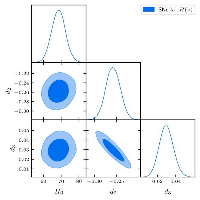
Figure 1: Contours for the joint analysis of SNe Ia and $H(z)$ data at 1$\sigma$ and 2$\sigma$ for the free parameters in the Comoving Distance parameterization (25).

III.1 Comoving Distance parameterization

In order to reconstruct the normalized torsion function (22) by using Supernovae and $H(z)$ data, we use the relation of Comoving Distance $D_{C}$ with magnitude $m$:

$$m=5\log_{10}\left[(1+z)D_{C}\right]+\mathcal{M},$$ (24)

where $\mathcal{M}$ is a constant, and write the parameterization of $D_{C}$ as:

$$D_{C}=z+d_{2}z^{2}+d_{3}z^{3}\,,$$ (25)

with $d_{2}$ and $d_{3}$ free parameters to be constrained, together the Hubble parameter $H_{0}$. Thus we have $\mathcal{O}=m$ and $\mathbf{p}=(H_{0},\,d_{2},\,d_{3})$. Using SNe Ia data for the magnitudes pantheon and Eqs. (23)-(25), $\chi^{2}_{m}$ is calculated.

By using (13) with Eq. (25) to obtain $E(z)$, we have:

$$E(z)=\frac{1}{1+2d_{2}z+3d_{3}z^{2}}\,,$$ (26)

so that $\mathcal{O}=H$ with $\mathbf{p}=(H_{0},\,d_{2},\,d_{3})$. By using the cosmic chronometers $H(z)$ data from Magana2018 , Eq. (23) can be combined with Eq. (26), and $\chi^{2}_{H}$ is calculated.

By probing the likelihood, $\mathscr{L}\propto e^{-\frac{1}{2}(\chi^{2}_{H}+\chi^{2}_{m})}$, $H_{0}$, $d_{2}$ and $d_{3}$ confidence plots were generated and are showed in Figure 1. As can be seen, the parameters are well constrained for the SNe Ia+$H(z)$ combined dataset. One can also realize that there is some correlation between parameters $d_{2}$ and $d_{3}$, while there is almost no correlation between $H_{0}$ and the other parameters. One can also realize that none of the parameters are negligible, as they are not compatible with zero, at least at 95% c.l.

From the MCMC chains corresponding to the parameters $(H_{0},d_{2},d_{3})$ and with the relations (25) and (26), we wanted to reconstruct the normalized torsion function $\Phi$ from the relation (22). However, as can be seen in (22), another parameter is needed to obtain $\Phi(z)$, namely, $\Omega_{m}$. As $\Omega_{m}$ is a dynamic parameter that can not be obtained from kinematic parametrizations, we chose to work with a Gaussian prior, $\Omega_{m}=0.315\pm 0.021$, which corresponds to 3$\sigma$ from the Planck estimate Planck2018 . The result of this reconstruction is shown in Figure 2.

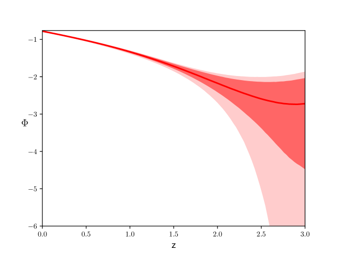
Figure 2: Reconstruction of the normalized torsion function $\Phi$ with the parameterization (25) for the Comoving Distance.

As can be seen from this Figure, in the context of this torsion model, the torsion can not be neglected at the considered redshift interval, which corresponds to the $H(z)$ and SNe Ia data redshifts.

The mean values of the free parameters are summarized in the table below:

Parameter	68% and 95% limits
$H_{0}$	$68.5\pm 3.9\pm 8$
$d_{2}$	$-0.258^{+0.016+0.033}_{-0.016-0.032}$
$d_{3}$	$0.0297^{+0.0077+0.016}_{-0.0077-0.015}$

Table 1: Mean values with 68% and 95% c.l. for the parameters $H_{0}$, $d_{2}$ and $d_{3}$ for the Comoving Distance parameterization.

We can see from this Table that these results are compatible with other results in the literature, as for instance, JesusEtAl18 , where it has been used the same parametrization, Eq. (25), and obtained $H_{0}=69.1\pm 1.5$ km/s/Mpc, $d_{2}=-0.253\pm 0.016$ and $d_{3}=0.0299\pm 0.0044$, at 1$\sigma$ c.l., which are all compatible within $1\sigma$ c.l. Concerning the current $H_{0}$ tension, this result is also compatible with the CMB result from Planck Planck2018 , $H_{0}=67.4\pm 0.5$ km/s/Mpc and the local result from SH0ES SH0ES22 , $H_{0}=73.04\pm 1.04$ km/s/Mpc. This compatibility with both results is due to the fact that the $H(z)$ data that we have used MorescoEtAl22 has included systematic errors, which increases the estimated uncertainty for $H_{0}$.

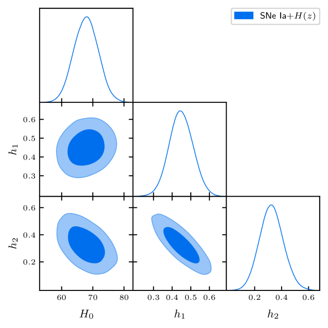
Figure 3: Contours for the joint analysis of SNe Ia and $H(z)$ data at 1$\sigma$ and 2$\sigma$ for the free parameters in the Hubble parameter parameterization (27).

III.2 $H(z)$ parametrization

Alternatively, we can also reconstruct $\Phi$ by means of the parameterization of the Hubble parameter:

$$H(z)=H_{0}(1+h_{1}z+h_{2}z^{2})\,,$$ (27)

with $\mathcal{O}=H$ and $\mathbf{p}=(H_{0},\,h_{1},\,h_{2})$. By using the $H(z)$ data from cosmic chronometers MorescoEtAl22 , Eq. (23) combined with Eq. (27), the $\chi^{2}_{H}$ function can be calculated. By using (13) with Eq. (27), the comoving distance is:

$$D_{C}(z)\equiv\int_{0}^{z}\frac{dz}{1+h_{1}z+h_{2}z^{2}},$$ (28)

which can be combined with Eq. (24) to calculate $\chi^{2}_{m}$ through SNe Ia data.

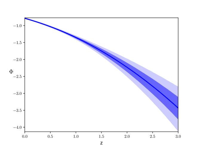
Figure 4: Reconstruction of the normalized torsion function $\Phi$ with the parameterization (27) for the comoving distance.

The likelihood function $\mathscr{L}\propto e^{-\frac{1}{2}(\chi^{2}_{H}+\chi^{2}_{m})}$ furnishes the contours of the parameters $H_{0}$, $h_{1}$ and $h_{2}$ for 1$\sigma$ and $2\sigma$ c.l., as shown in Figure 3. As can be seen from this Figure, the free parameters are well constrained by the combination of SNe Ia+$H(z)$ data. The main correlation is between parameters $h_{1}$ and $h_{2}$. There is also some correlation between $H_{0}$ and $h_{2}$. The mean values and 68% and 95% c.l. for the free parameters are presented in Table 2.

Parameter	68% and 95% limits
$H_{0}$	$67.8\pm 3.9\pm 8$
$h_{1}$	$0.448\pm 0.064\pm 0.13$
$h_{2}$	$0.325^{+0.089+0.18}_{-0.089-0.17}$

Table 2: Mean values and 68% and 95% c.l. for the parameters $H_{0}$, $h_{1}$ and $h_{2}$ for the Hubble parameter parameterization.

The results shown in Table 2 can be compared with a previous analysis in the context of the same $H(z)$ parametrization. In JesusEtAl18 , they have obtained $H_{0}=68.8\pm 1.6$ km/s/Mpc, $h_{1}=0.522\pm 0.065$ and $h_{2}=0.192\pm 0.026$. $H_{0}$ and $h_{1}$ are compatible within 1$\sigma$ c.l., while $h_{2}$ is compatible only at 2$\sigma$ c.l. This result for $H_{0}$ is also compatible with the CMB result from Planck Planck2018 , $H_{0}=67.4\pm 0.5$ km/s/Mpc, within 1$\sigma$ c.l., and with the local result from SH0ES SH0ES22 , $H_{0}=73.04\pm 1.04$ km/s/Mpc, within $2\sigma$ c.l.

From the MC chains corresponding to the parameters $(H_{0},h_{1},h_{2})$ and with the relations (28) and (27), we reconstructed the normalized torsion function $\Phi$ from the relation (22). We have also used the 3$\sigma$ Planck prior, $\Omega_{m}=0.315\pm 0.021$. This is shown in Figure 4.

As can be seen from this Figure, the torsion is well reconstructed from the comoving distance parametrization.

The concordance between the two reconstructions above can be seen in Figure 5, where the $1\sigma$ interval for both cases are shown in the same figure. We see that both reconstructions are in good agreement within $1\sigma$ c.l.

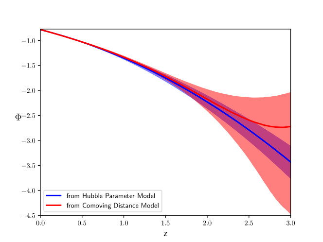
Figure 5: Superposition of the two different reconstructions for $\Phi$ within $1\sigma$ c.l.

III.3 Deceleration Parameter

In order to validate the discussed torsion model as a candidate to describe the dark energy sector, we reconstruct the deceleration parameter $q$ in order to compare to the standard model one. From (4) we obtain:

$$q(z)=-1+\left(1+z\right)\dfrac{H^{\prime}}{H}\,.$$ (29)

Using this expression, it is easy to show that for the comoving distance parametrization (25), with $E(z)$ given by Eq. (26), the deceleration parameter is given by:

$$q(z)=-1-\frac{(1+z)(2d_{2}+6d_{3}z)}{1+2d_{2}z+3d_{3}z^{2}}$$ (30)

Similarly, it is easy to show that for the $H(z)$ parametrization (27), the deceleration parameter is given by:

$$q(z)=-1+\frac{(1+z)(h_{1}+2h_{2}z)}{1+h_{1}z+h_{2}z^{2}}$$ (31)

Having the MCMC chains of the parameters $d_{2},\,d_{3}$ and $h_{1},\,h_{2}$ for both parametrizations, these expressions can be used to reconstruct $q(z)$ and the results are plotted, showing 1$\sigma$ confidence intervals, in Figure 6.

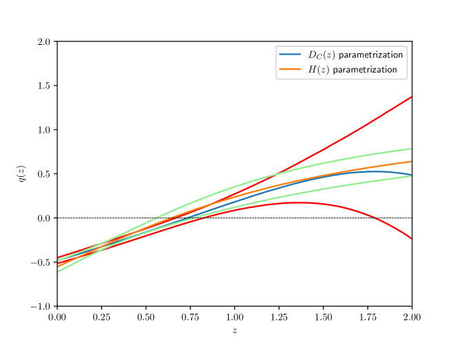
Figure 6: Reconstruction of the deceleration parameter $q(z)$ for the two parametrizations: $D_{C}(z)$ (median in blue) and 1$\sigma$ confidence interval (red) and $H(z)$ (median in orange) and 1$\sigma$ confidence interval (green).

It is evident from this figure that the transition redshift $z_{t}$ occurs at about $0.60-0.75$, in good agreement, for instance, with the value of $z_{t}\simeq 0.67$ for the standard $\Lambda$CDM model with $\Omega_{m}\simeq 0.3$ and $\Omega_{\Lambda}\simeq 0.7$.

IV Concluding remarks

We have studied the torsion effects in Cosmology as a candidate to dark energy in the Universe. The analysis was done by assuming that the torsion function $\phi(t)$ drives the recent cosmic evolution, and contrary to recent works where the specific form of the torsion function were fixed, here we have reconstructed the torsion function by using observational data of Supernovae and Hubble parameter measurements. The method of reconstruction was based on a cosmographic analysis, where previous parametrizations for the comoving distance and the Hubble parameter are adopted and the free parameters of the models are constrained by observational data. The values of the free parameters are then used to reconstruct the normalized torsion function $\Phi(z)$, without to appeal to a specific cosmological model. The value of the $H_{0}$ parameter (within $2\sigma$ c.l.) obtained by the two parametrizations are in good agreement to both recent estimates, namely measures obtained by the local distance ladder and by the cosmic microwave background power spectrum. However, there is a slight preference for the later one, as it is compatible within 1$\sigma$, while the first one is compatible within 2$\sigma$ only. The estimate of the deceleration parameter is also in good agreement to the standard model estimate. Such interesting features show that torsion effect in the evolution of the universe must be further investigated.

- (1)
- Farooq et al. (2017) O. Farooq, F. R. Madiyar, S. Crandall, and B. R., Astrophys. J. 835, 26 (2017), eprint 1607.03537.
- Scolnic et al. (2018) D. M. Scolnic et al., Astrophys. J. 859, 101 (2018), eprint 1710.00845.
- Aghanim et al. (2020) N. Aghanim et al. (Planck), Astron. Astrophys. 641, A6 (2020), eprint 1807.06209.
- Riess (2019) A. G. Riess, Nature Rev. Phys. 2, 10 (2019), eprint 2001.03624.
- Martinelli and Tutusaus (2019) M. Martinelli and I. Tutusaus, Symmetry 11, 986 (2019), eprint 1906.09189.
- Bull et al. (2016) P. Bull et al., Phys. Dark Univ. 12, 56 (2016), eprint 1512.05356.
- Pasmatsiou et al. (2017) K. Pasmatsiou, C. G. Tsagas, and J. D. Barrow, Phys. Rev. D 95, 104007 (2017), eprint 1611.07878.
- Kranas et al. (2019) D. Kranas, C. G. Tsagas, J. D. Barrow, and D. Iosifidis, Eur. Phys. J. C 79, 341 (2019), eprint 1809.10064.
- Pereira et al. (2019) S. H. Pereira, R. d. C. Lima, J. F. Jesus, and R. F. L. Holanda, Eur. Phys. J. C 79, 950 (2019), eprint 1906.07624.
- Barrow et al. (2019) J. D. Barrow, C. G. Tsagas, and G. Fanaras, Eur. Phys. J. C 79, 764 (2019), eprint 1907.07586.
- Mehdizadeh and Ziaie (2019) M. R. Mehdizadeh and A. H. Ziaie, Phys. Rev. D 99, 064033 (2019), eprint 1811.03364.
- Medina et al. (2019) S. B. Medina, M. Nowakowski, and D. Batic, Annals Phys. 400, 64 (2019), eprint 1812.04589.
- Luz and Carloni (2019) P. Luz and S. Carloni, Phys. Rev. D 100, 084037 (2019), eprint 1907.11489.
- Khakshournia and Mansouri (2019) S. Khakshournia and R. Mansouri, Class. Quant. Grav. 36, 227001 (2019), eprint 1912.12650.
- Marques and Martins (2020) C. M. J. Marques and C. J. A. P. Martins, Phys. Dark Univ. 27, 100416 (2020), eprint 1911.08232.
- Bose and Chakraborty (2020) A. Bose and S. Chakraborty, Eur. Phys. J. C 80, 205 (2020), eprint 2003.07226.
- Bolejko et al. (2020) K. Bolejko, M. Cinus, and B. F. Roukema, Phys. Rev. D 101, 104046 (2020), eprint 2003.06528.
- Izaurieta and Lepe (2020) F. Izaurieta and S. Lepe, Class. Quant. Grav. 37, 205004 (2020), eprint 2004.06058.
- Cabral et al. (2020) F. Cabral, F. S. N. Lobo, and D. Rubiera-Garcia, JCAP 10, 057 (2020), eprint 2004.13693.
- Cruz et al. (2020) M. Cruz, F. Izaurieta, and S. Lepe, Eur. Phys. J. C 80, 559 (2020), eprint 2005.04550.
- Shaposhnikov et al. (2020) M. Shaposhnikov, A. Shkerin, I. Timiryasov, and S. Zell, JHEP 10, 177 (2020), eprint 2007.16158.
- Shaposhnikov et al. (2021a) M. Shaposhnikov, A. Shkerin, I. Timiryasov, and S. Zell, Phys. Rev. Lett. 126, 161301 (2021a), [Erratum: Phys.Rev.Lett. 127, 169901 (2021)], eprint 2008.11686.
- Shaposhnikov et al. (2021b) M. Shaposhnikov, A. Shkerin, I. Timiryasov, and S. Zell, JCAP 02, 008 (2021b), [Erratum: JCAP 10, E01 (2021)], eprint 2007.14978.
- Bondarenko et al. (2021) S. Bondarenko, S. Pozdnyakov, and M. A. Zubkov, Eur. Phys. J. C 81, 613 (2021), eprint 2009.05571.
- Karananas et al. (2021) G. K. Karananas, M. Shaposhnikov, A. Shkerin, and S. Zell, Phys. Rev. D 104, 064036 (2021), eprint 2106.13811.
- Guimarães et al. (2021) T. M. Guimarães, R. d. C. Lima, and S. H. Pereira, Eur. Phys. J. C 81, 271 (2021), eprint 2011.13906.
- Kasem and Khalil (2022) A. Kasem and S. Khalil, EPL 139, 19002 (2022), eprint 2012.09888.
- Pereira et al. (2022) S. H. Pereira, A. M. Vicente, J. F. Jesus, and R. F. L. Holanda, Eur. Phys. J. C 82, 356 (2022), eprint 2202.01807.
- Elizalde et al. (2023) E. Elizalde, F. Izaurieta, C. Riveros, G. Salgado, and O. Valdivia, Phys. Dark Univ. 40, 101197 (2023), eprint 2204.00090.
- Liu et al. (2023) T. Liu, Z. Liu, J. Wang, S. Gong, M. Li, and S. Cao (2023), JCAP 07, 059 (2023), eprint 2304.06425.
- Akhshabi and Zamani (2023) S. Akhshabi and S. Zamani (2023), Gen. Rel. Grav. 55, 102 (2023), eprint 2305.00415.
- Visser (2004) M. Visser, Class. Quant. Grav. 21, 2603 (2004), eprint gr-qc/0309109.
- Visser (2005) M. Visser, Gen. Rel. Grav. 37, 1541 (2005), eprint gr-qc/0411131.
- Shapiro and Turner (2006) C. Shapiro and M. S. Turner, Astrophys. J. 649, 563 (2006), eprint astro-ph/0512586.
- Blandford et al. (2005) R. D. Blandford, M. A. Amin, E. A. Baltz, K. Mandel, and P. J. Marshall, ASP Conf. Ser. 339, 27 (2005), eprint astro-ph/0408279.
- Elgaroy and Multamaki (2006) O. Elgaroy and T. Multamaki, JCAP 09, 002 (2006), eprint astro-ph/0603053.
- Rapetti et al. (2007) D. Rapetti, S. W. Allen, M. A. Amin, and R. D. Blandford, Mon. Not. Roy. Astron. Soc. 375, 1510 (2007), eprint astro-ph/0605683.
- Riess et al. (2007) A. G. Riess et al., Astrophys. J. 659, 98 (2007), eprint astro-ph/0611572.
- Rezaei et al. (2021) M. Rezaei, J. Solà Peracaula, and M. Malekjani, Mon. Not. Roy. Astron. Soc. 509, 2593 (2021), eprint 2108.06255.
- Mehrabi and Rezaei (2021) A. Mehrabi and M. Rezaei, Astrophys. J. 923, 274 (2021), eprint 2110.14950.
- Velasquez-Toribio and Fabris (2022) A. M. Velasquez-Toribio and J. C. Fabris, Braz. J. Phys. 52, 115 (2022), eprint 2104.07356.
- Lobo et al. (2020) F. S. N. Lobo, J. P. Mimoso, and M. Visser, JCAP 04, 043 (2020), eprint 2001.11964.
- Seikel et al. (2012) M. Seikel, C. Clarkson, and M. Smith, JCAP 06, 036 (2012), eprint 1204.2832.
- Holsclaw et al. (2010) T. Holsclaw, U. Alam, B. Sanso, H. Lee, K. Heitmann, S. Habib, and D. Higdon, Phys. Rev. D 82, 103502 (2010), eprint 1009.5443.
- Jesus et al. (2020) J. F. Jesus, R. Valentim, A. A. Escobal, and S. H. Pereira, JCAP 04, 053 (2020), eprint 1909.00090.
- Shafieloo et al. (2012) A. Shafieloo, A. G. Kim, and E. V. Linder, Phys. Rev. D 85, 123530 (2012), eprint 1204.2272.
- Li et al. (2007) C. Li, D. E. Holz, and A. Cooray, Phys. Rev. D 75, 103503 (2007), eprint astro-ph/0611093.
- Sahlen et al. (2005) M. Sahlen, A. R. Liddle, and D. Parkinson, Phys. Rev. D 72, 083511 (2005), eprint astro-ph/0506696.
- Mukherjee and Banerjee (2021) P. Mukherjee and N. Banerjee, Phys. Rev. D 103, 123530 (2021), eprint 2105.09995.
- von Marttens et al. (2021) R. von Marttens, J. E. Gonzalez, J. Alcaniz, V. Marra, and L. Casarini, Phys. Rev. D 104, 043515 (2021), eprint 2011.10846.
- Mukherjee and Mukherjee (2021) P. Mukherjee and A. Mukherjee, Mon. Not. Roy. Astron. Soc. 504, 3938 (2021), eprint 2104.06066.
- (53) W. T. Reid, Riccati Differential Equations, London: Academic Press (1972).
- (54) D. M. Scolnic et al., Astrophys. J. 859, 101 (2018), [arXiv:1710.00845 [astro-ph.CO]].
- (55) J. Magana, M. H. Amante, M. A. Garcia-Aspeitia and V. Motta, Mon. Not. Roy. Astron. Soc. 476, 1036 (2018), [arXiv:1706.09848 [astro-ph.CO]].
- (56) J. Goodman and J. Weare, Communications in Applied Mathematics and Computational Science 5, 33, 65 (2010).
- (57) Foreman-Mackey, D. W. Hogg, D. Lang and J. Goodman, Publications of the ASP 125, 306 (2013), [arXiv:1202.3665 [astro-ph.IM]].
- (58) M. Betoule et.al., A&A 568, A22 (2014), [arXiv:1401.4064 [astro-ph.CO]].
- (59) J. F. Jesus, R. F. L. Holanda and S. H. Pereira, JCAP 05 (2018), 073 [arXiv:1712.01075 [astro-ph.CO]].
- (60) J. F. Jesus, R. Valentim, P. H. R. S. Moraes and M. Malheiro, Mon. Not. Roy. Astron. Soc. 500 (2020) no.2, 2227-2235 [arXiv:1907.01033 [astro-ph.CO]].
- (61) Planck Collaboration: N. Aghanim et al. Astron. Astrophys. 641, A6 (2020), [arXiv:1807.06209 [astro-ph.CO]].
- (62) A. G. Riess, W. Yuan, L. M. Macri, D. Scolnic, D. Brout, S. Casertano, D. O. Jones, Y. Murakami, L. Breuval and T. G. Brink, et al. Astrophys. J. Lett. 934 (2022) no.1, L7 [arXiv:2112.04510 [astro-ph.CO]].
- (63) M. Moresco, L. Amati, L. Amendola, S. Birrer, J. P. Blakeslee, M. Cantiello, A. Cimatti, J. Darling, M. Della Valle and M. Fishbach, et al. Living Rev. Rel. 25 (2022) no.1, 6 [arXiv:2201.07241 [astro-ph.CO]].