Helmholtz quasi-resonances are unstable under most single-signed perturbations of the wave speed

Abstract.

We consider Helmholtz problems with a perturbed wave speed, where the single-signed perturbation is governed by a parameter $z$. Both the wave speed and the perturbation are allowed to be discontinuous (modelling a penetrable obstacle). We show that, for any frequency, for most values of $z$, the solution operator is polynomially bounded in the frequency.

This solution-operator bound is most interesting for Helmholtz problems with strong trapping; recall that here there exist a sequence of real frequencies, tending to infinity, through which the solution operator grows superalgebraically, with these frequencies often called quasi-resonances. The result of this paper then shows that, at every quasi-resonance, the superalgebraic growth of the solution operator does not occur for most single-signed perturbations of the wave speed, i.e., quasi-resonances are unstable under most such perturbations.

1. Introduction

1.1. The main results

Let $\Delta$ be the Laplace operator on $\mathbb{R}^{d}$. Let $n\in L^{\infty}(\mathbb{R}^{d};\mathbb{R})$ be strictly positive and equal to $1$ outside a sufficiently-large ball. Let $\psi\in L^{\infty}_{\rm comp}(\mathbb{R}^{d};\mathbb{R})$. Let $R_{0}>0$ be such that $\operatorname{supp}(1-n)\cup\operatorname{supp}(\psi)\subset B(0,R_{0})$.

Given $k>0$, $z\in\mathbb{R}$, and $f\in L^{2}_{\rm comp}(\mathbb{R}^{d})$, let $u\in H^{1}_{\rm loc}(\mathbb{R}^{d})$ be the outgoing solution to

(1.1) $$(-k^{-2}\Delta-n-z\psi)u=f,$$

where $u$ is outgoing if it satisfies the Sommerfeld radiation condition that

(1.2) $$\left(k^{-1}\frac{\partial}{\partial r}-i\right)u=o(r^{-(d-1)/2})\quad\text{ as }r:=|x|\to\infty,\text{ uniformly in }x/r.$$

With the Helmholtz equation (1.1) understood as coming from the wave equation via Fourier transform in time (with Fourier variable $k$), $n+z\psi$ is then the inverse of the square of the wave speed.

The existence and uniqueness of the solution to (1.1)-(1.2) is standard (see the recap in Lemma 2.1 below). We then write $u=(-k^{-2}\Delta-n-z\psi-i0)^{-1}f$, where the $i0$ indicates that the radiation condition can be obtained by the limiting absorption principle (see Lemma 2.1 below).

This paper is concerned with the behaviour of the solution operator $\chi(-k^{-2}\Delta-n-z\psi-i0)^{-1}\chi:L^{2}\to L^{2}$, where $\chi\in C^{\infty}_{\rm comp}(\mathbb{R}^{d})$, as a function of both the frequency $k>0$ and the perturbation parameter $z$.

We recall that the high-frequency behaviour of the solution operator $\chi(-k^{-2}\Delta-n)^{-1}\chi$ with smooth $n$ is closely linked to the dynamics of the Hamiltonian system with Hamiltonian

(1.3) $$p(x,\xi)={\lvert{\xi}\rvert}^{2}-n(x).$$

Letting $\Sigma$ denote the characteristic set, a.k.a., the energy surface,

$$\Sigma:=\big{\{}(x,\xi):p(x,\xi)=0\big{\}},$$

we consider the dynamics inside $\Sigma$ given by the flow along the Hamilton vector field

$$H_{p}:=2\xi\cdot{\partial}_{x}+\nabla n\cdot{\partial}_{\xi}.$$

(This is Newton’s second law, with force given by the gradient of the potential $-n$.) The integral curves of $H_{p}$, i.e., the solutions $(x(t),\xi(t))$ of

$$\frac{dx_{i}}{dt}=2\xi_{i}\quad\text{ and }\quad\frac{d\xi_{i}}{dt}=\frac{\partial n}{\partial x_{i}},$$

in $\Sigma$ are known as null bicharacteristics. A null bicharacteristic is said to be trapped forwards/backwards if

$$\lim_{t\to\pm\infty}{\lvert{x(t)}\rvert}\neq\infty.$$

We say that a set $S\subset\mathbb{R}^{d}$ geometrically controls the backward trapped null bicharacteristics if for each $(x(0),\xi(0))$ on a backward trapped null bicharacteristic $(x(t),\xi(t))$, there exists $T<0$ with $x(T)\in S$.

Theorem 1.1 (Main result for smooth $n$).

Suppose that, in addition to the assumptions on $n$ and $\psi$ above, $n,\psi\in C^{\infty}$ and $\psi\geq c>0$ on a set that geometrically controls all backward-trapped null bicharacteristics for $-k^{-2}\Delta-n$.

(a) Given $\epsilon,k_{0},\rho>0$ and $\chi\in C^{\infty}_{\rm comp}(\mathbb{R}^{d})$, there exists $C_{1}>0$ such that, for all $k\geq k_{0}$, $z\mapsto\chi(-k^{-2}\Delta-n-z\psi-i0)^{-1}\chi$ extends meromorphically from $z\in(-\rho,\rho)$ to $z\in\mathbb{C}$, with the number of poles in $\{z\in\mathbb{C},|z|<\rho\}$ bounded by $C_{1}k^{d+1+\epsilon}$.

(b) There exists $\rho>0$ such that the following is true. Given $\epsilon,k_{0},\delta>0$, $N\geq 0$, and $\chi\in C^{\infty}_{\rm comp}(\mathbb{R}^{d})$, there exists $C_{2}>0$ such that for all $k\geq k_{0}$ there exists a set $S_{k}\subset(-\rho,\rho)$ with $|S_{k}|\leq\delta k^{-N}$ such that

(1.4) $$\|\chi(-k^{-2}\Delta-n-z\psi-i0)^{-1}\chi\|_{L^{2}\to L^{2}}\leq\frac{C_{2}}{\delta}k^{5(d+1)/2+N+\epsilon}\text{ for all }z\in(-\rho,\rho)\setminus S_{k}.$$

When $N=0$ in Part (b) of Theorem 1.1, the set of $z$ excluded in (1.4) has arbitrarily small measure, independent of $k$. Choosing $N>0$ allows one to decrease the measure of this excluded set as $k$ increases (at the price of a larger exponent in the bound).

Theorem 1.2 (Main result for discontinuous $n$).

Given $\mathcal{O}$ compact and Lipschitz and $n_{i}>0$, let

(1.5) $$n:=\begin{cases}n_{i}&\text{ in }\mathcal{O},\\ 1&\text{ in }\mathbb{R}^{d}\setminus\mathcal{O}\end{cases}$$

Suppose that $\operatorname{supp}\psi\supset\mathcal{O}$ and there exists $c>0$ such that $\psi\geq c$ on $\mathcal{O}$ (observe that this includes the case $\psi=1_{\mathcal{O}}$).

(a) Given $\rho,k_{0}>0$ and $\chi\in C^{\infty}_{\rm comp}(\mathbb{R}^{d})$, there exists $C_{1}>0$ such that, for all $k\geq k_{0}$, $z\mapsto\chi(-k^{-2}\Delta-n-z\psi-i0)^{-1}\chi$ extends meromorphically from $z\in(-\rho,\rho)$ to $z\in\mathbb{C}$, with the number of poles in $\{z\in\mathbb{C},|z|<\rho\}$ bounded by $C_{1}k^{d+2}$.

(b) Given $\rho,\epsilon,k_{0},\delta>0$, $N\geq 0$, and $\chi\in C^{\infty}_{\rm comp}(\mathbb{R}^{d})$, there exist $C_{2}>0$ such that for all $k\geq k_{0}$ there exists a set $S_{k}\subset(-\rho,\rho)$ with $|S_{k}|\leq\delta k^{-N}$ such that

(1.6) $$\|\chi(-k^{-2}\Delta-n-z\psi-i0)^{-1}\chi\|_{L^{2}\to L^{2}}\leq\frac{C_{2}}{\delta}k^{2+5(d+3)/2+N+\epsilon}\text{ for all }z\in(-\rho,\rho)\setminus S_{k}.$$

We highlight that the dynamical assumption in Theorem 1.2 is related to that in Theorem 1.1. Indeed, in the case of discontinuous, piecewise-constant $n$ (as in (1.5)), the dynamics of null bicharacteristics is that of straight-line motion (arising from a constant potential) away from the obstacle, but internal refraction at the boundary can produce trapping of rays in the manner of whispering gallery solutions (see, e.g., [PV99] and §1.2 below). The assumption of Theorem 1.2 that $\psi$ is strictly positive on the obstacle therefore implies that it is strictly positive on all the backwards trapped null bicharacteristics, and hence geometrically controls them.

1.2. Application of the main results to problems with quasi-resonances

When $n(x)$ is a sufficiently-quickly decreasing function of $|x|$, then $\chi(-k^{-2}\Delta-n-i0)^{-1}\chi$ has poles (i.e., resonances) as a function of (the complex extension of) $k$ that are close to the real axis.

Indeed, [Ral71, Theorem 1] showed that if $n\in C^{\infty}$ is radial and $|x|\sqrt{n(|x|)}$ is not monotonically increasing (i.e., at some point $n(x)$ decreases faster than $|x|^{-2}$), then there exist a sequence of poles of $\chi(-k^{-2}\Delta-n-i0)^{-1}\chi$ exponentially close to the real axis. In the penetrable-obstacle case, if $\mathcal{O}$ is smooth and uniformly convex and $n_{i}>1$ then [PV99, Theorem 1.1] showed that there exist a sequence of poles of $\chi(-k^{-2}\Delta-n-i0)^{-1}\chi$ superalgebraically close to the real axis; these are related to the classic “whispering-gallery modes” (see, e.g., [BB91]).

By [Ste00, Theorem 1], the existence of poles superalgebraically close to real axis implies the existence of quasimodes with superalgebraically small error; i.e., in both the cases mentioned above, there exist $\{k_{j}\}_{j=1}^{\infty}$, with $k_{j}\to\infty$ as $j\to\infty$, such that, given $N>0$ there exists $C_{N}>0$ such that

(1.7) $$\|\chi(-k_{j}^{-2}\Delta-n-i0)^{-1}\chi\|_{L^{2}\to L^{2}}\geq C_{N}(k_{j})^{N};$$

these $k_{j}$ are often called quasi-resonances. (Note that, in the penetrable-obstacle case when $\mathcal{O}$ is a ball, exponential growth of the solution operator through the quasi-resonances is shown in [Cap12, CLP12, AC18].)

The bound (1.4) and (1.6) applied to the two situations above with $k=k_{j}$ show that at every quasi-resonance the superalgebraic growth (1.7) is disrupted by the perturbation for most $z$ (more precisely, for all $z$ apart from a set of arbitrarily small measure); i.e., at a quasi-resonance, the superalgebraic growth does not occur for most single-signed perturbations of the wave speed.

This instability of the growth through quasi-resonances is illustrated qualitatively for low frequencies in Figures 1.1 and 1.2 in the setting of Theorem 1.2. Figures 1.1 and 1.2 both plot the absolute value of the wave scattered by an incident plane wave for $n=n_{i}1_{\mathcal{O}}$, $\psi=1_{\mathcal{O}}$, and $\mathcal{O}=B(0,1)$. In this case, the solution can be written down explicitly in terms of Fourier series and Bessel/Hankel functions, and the quasi-resonances expressed as zeros of a combination of Bessel/Hankel functions. At least for small $k$, both the quasi-resonances and the solution can thereby computed be accurately; this was done in [MS19, §6.2], and Figures 1.1 and 1.2 are plotted using the same MATLAB code.

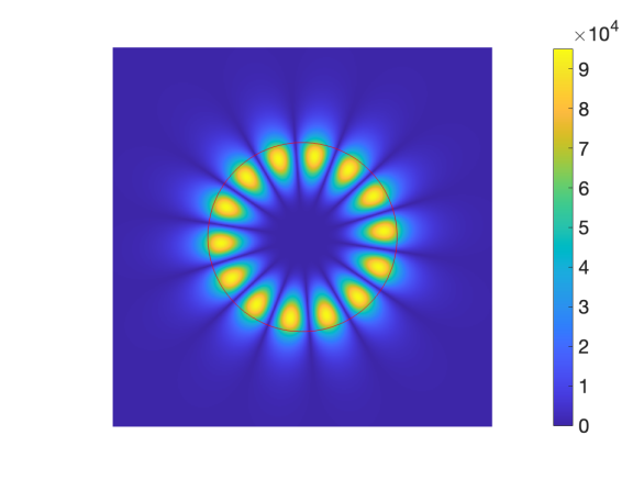
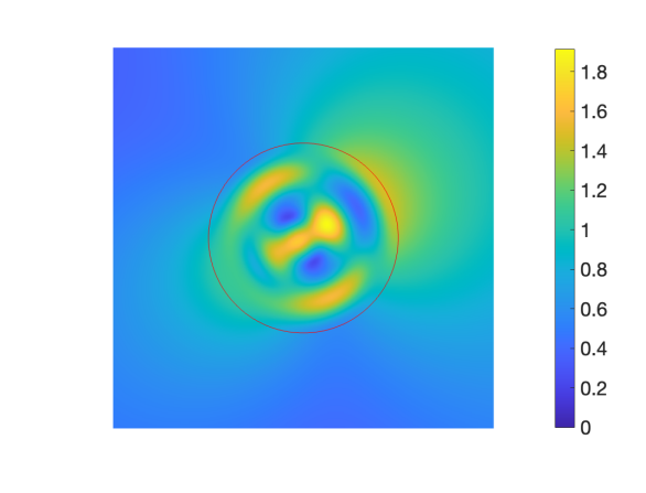
$n_{i}=100$, $z=0$                                     $n_{i}=100$, $z=0.01$

Figure 1.1. The absolute value of the field scattered by the plane wave $\exp(ik(x\cos(\pi/6)+y\sin(\pi/6)))$ hitting the penetrable obstacle $\mathcal{O}=B(0,1)$ with $n_{i}=100$ (the red line denotes the boundary $\mathcal{O}$.) The frequency $k=0.992772133752486$, which is (an approximation to) a quasi-resonance for the problem when $n_{i}=100$. The left plot corresponds to $n_{i}=100$ and $z=0$ (i.e., the setting of the quasi-resonance) and the right plot corresponds to $n_{i}=100$ and $z=0.01$ (i.e., a small perturbation of the wave speed). We highlight the different scales on the colour bars.

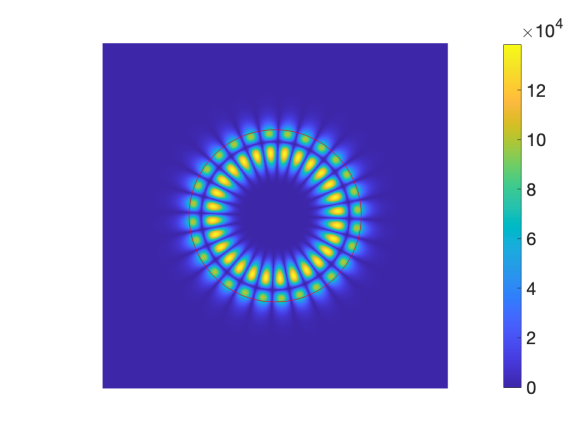
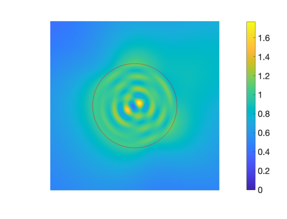
$n_{i}=100$, $z=0$                                     $n_{i}=100$, $z=0.01$

Figure 1.2. Same as Figure 1.1 except now $k=2.19476917403094$, which is also (an approximation to) a quasi-resonance when $n_{i}=100$.

There has been sustained interest in the mathematics and physics communities in studying the stability/perturbation of resonances. Quantitative results about how the resonances behave under small perturbations of the wave speed and/or domain in specific situations are given in, e.g, [Rau80] [AHK84, §3], [HS96, HBKW08, McH17, ADFM20, ADFM21], and rather general results about resonance stability and simplicity under perturbation are given by, e.g., [Ste94, KZ95, AT04, Sjö14, Xio23]. Theorems 1.1 and 1.2 give a new perspective, complementary to these existing ones, on the (in)stability of resonances under perturbations of the wave speed. The next subsection describes how Theorems 1.1 and 1.2 are proved using techniques originally introduced to show that existence of quasimodes with superalgebraically small error implies existence of resonances superalgebraically close to the real axis [SV95, SV96, TZ98].

1.3. The ideas behind the proofs of Theorems 1.1 and 1.2

Part (b) of Theorem 1.1/1.2 can be viewed as a counterpart to the solution-operator bound in [LSW21, Theorem 3.3]. Indeed [LSW21, Theorem 3.3] showed that the solution operator for a wide variety of scattering problems is polynomially bounded in $k$ for “most” $k$ . Applied to a problem with quasi-resonances, this result shows that the superalgebraic growth of the solution through $\{k_{j}\}_{j=1}^{\infty}$ is unstable with respect to “most” perturbations in $k$. Part (b) of Theorem 1.1/1.2 shows that this superalgebraic growth is unstable with respect to “most” single-signed perturbations of the wave speed.

The proofs of Part (b) of Theorem 1.1/1.2 follow the same outline as the proof of [LSW21, Theorem 3.3]. Indeed, the ingredients of the proof of [LSW21, Theorem 3.3] are

1. the semiclassical maximum principle – a consequence of the Hadamard three-lines theorem of complex analysis, and originally used in [TZ98],

2. a bound on the number of poles of $(P-z)^{-1}$ where $P=-k^{-2}n^{-1}\Delta$ – see [DZ19, Theorems 4.13 and 7.4] and the overview in [DZ19, §7.6] on the large literature on proving such a bound,

3. a bound on $(P-z)^{-1}$, with $z$ a prescribed distance away from poles (coming from [SV95, SV96, TZ98]), and

4. the bound $\|(P-z)^{-1}\|_{L^{2}\to L^{2}}\leq 1/(\operatorname{Im}z)$ for $\operatorname{Im}z>0$, coming, e.g., from considering the pairing $\langle(P-z)u,u\rangle_{L^{2}}$ and then using self-adjointness of $P$.

In our setting, however, we need to prove analogues of (2)-(4) with the additional complication that the perturbation $z\psi$, unlike a spectral parameter, is not supported everywhere (since $\psi$ has compact support). Note that the analogue of Point (2) is then Part (a) of Theorems 1.1 and 1.2.

The assumption in Theorems 1.1 and 1.2 that $\psi>0$ in a suitable region comes from Ingredient (4) – this sign condition on $\psi$ ensures there is a half-space in $z$ where one can obtain a bound with $1/(\operatorname{Im}z)$ on the right-hand side (see Lemmas 3.2 and 3.3 below). Indeed, the imaginary part of the pairing $\langle(-k^{-2}\Delta-n-z\psi)u,u\rangle_{L^{2}}$ gives information about $u$ on the support of $\psi$; we then propagate this information off $\operatorname{supp}\psi$ via a commutator argument. In the proof of Theorem 1.1 this commutator argument occurs in the setting of (semiclassical) defect measures (with our default references [Zwo12, DZ19]); see Lemma 3.2 below. In the proof of Theorem 1.2 we commute with $x\cdot\nabla$ (plus lower-order terms); see Lemma 3.3 below. Recall that this commutator was pioneered by Morawetz in the setting of obstacle scattering [ML68, Mor75], with the ideas recently transposed to the penetrable obstacle case in [MS19].

1.4. Discussion of Theorems 1.1 and 1.2 in the context of uncertainty quantification

One motivation for proving Theorems 1.1 and 1.2 comes from uncertainty quantification (UQ). The forward problem in UQ of PDEs is to compute statistics of quantities of interest involving PDEs either posed on a random domain or having random coefficients.

A crucial role in UQ theory is understanding regularity of the solution $u$ with respect to $y$, where $y$ is a vector of parameters governing the randomness and the problem is posed in the abstract form $P(y)u(y)=f$, with $P$ a differential or integral operator. Indeed, some of the strongest UQ convergence results are obtained by proving that $u$ is holomorphic with respect to (the complex extension of) $y$, or by proving equivalent bounds on the derivatives; see, e.g., [CDS10, Theorem 4.3], [CDS11], [KS13, Section 2.3]. This parametric holomorphy allows one to establish rates of convergence for stochastic-collocation/sparse-grid schemes, see, e.g., [CCS15, CCNT16, HAHPS18], quasi-Monte Carlo (QMC) methods, see, e.g., [Sch13, DKLG⁺14, DKLGS16, KN16, HPS16], Smolyak quadratures, see, e.g., [ZS20], and deep-neural-network approximations of the solution; see, e.g., [SZ19, OSZ21, LMRS21].

At least for the Dirichlet obstacle problem, existence of super-algebraically small quasimodes for $\chi(-k^{-2}\Delta-1-i0)^{-1}\chi$ (i.e., (1.7)) implies the existence of a pole of $z\mapsto\chi(-k^{2}\Delta-1-z1_{B(0,R)}-i0)^{-1}\chi$ superalgebraically-close to the origin by [GMS21, Theorem 1.5] (see also [SW23, Theorem 1.11]); we expect the analogous result to be true for the variable-wave-speed problem (1.1) when $n$ is smooth (indeed, the propagation arguments are simpler in the case when there is no boundary).

Part (a) of Theorem 1.1 and Part (a) of Theorem 1.2 immediately imply that, given $k>0$, for “most” $z\in(-\epsilon,\epsilon)$ the map $z\mapsto\chi(-k^{-2}\Delta-n-z\psi-i0)^{-1}\chi$ is holomorphic in a ball of radius $\sim k^{-M}$; i.e., the bad behaviour exhibited above by [GMS21, Theorem 1.5] is rare.

Corollary 1.3 (Holomorphy of solution operator in $B(z,Ck^{-M})$ for “most” $z$).

(a) Under the assumptions of Theorem 1.1, given $\rho,\epsilon,\delta,k_{0}>0$ and $\chi\in C^{\infty}_{\rm comp}(\mathbb{R}^{d})$, there exists $C>0$ such that, for all $k\geq k_{0}$, there exists $S_{k}\subset(-\rho,\rho)$ with $|S_{k}|<\delta$ such that for all $z\in(-\rho,\rho)\setminus S_{k}$, the map $z\mapsto\chi(-k^{-2}\Delta-n-z\psi)^{-1}\chi$ is holomorphic in $B(z,Ck^{-(d+1+\epsilon)})$.

(b) Under the assumptions of Theorem 1.2, given $\rho,\delta,k_{0}>0$ and $\chi\in C^{\infty}_{\rm comp}(\mathbb{R}^{d})$, there exists $C>0$ such that, for all $k\geq k_{0}$, there exists $S_{k}\subset(-\rho,\rho)$ with $|S_{k}|<\delta$ such that for all $z\in(-\rho,\rho)\setminus S_{k}$, the map $z\mapsto\chi(-k^{-2}\Delta-n-z\psi)^{-1}\chi$ is holomorphic in $B(z,Ck^{-(d+2)})$.

Proof.

We prove the result in Part (a); the proof of the result in Part (b) is completely analogous. By Theorem 1.1, given $\epsilon>0$, in a $k$-independent neighbourhood of $(-\rho,\rho)$ there are at most $C_{1}k^{d+1+\epsilon}$ poles $\mathcal{P}$. Let $C:=\delta/(2C_{1})$, and let

$$S_{k}:=\bigcup_{p\in\mathcal{P}}(-\rho,\rho)\cap B(p,Ck^{-(d-1-\epsilon)}).$$

Then, since $|(-\rho,\rho)\cap B(p,Ck^{-(d-1-\epsilon)})|\leq 2Ck^{-(d-1-\epsilon)}\leq\delta C_{1}^{-1}k^{-(d-1-\epsilon)}$ for any $p$, we have $|S_{k}|\leq|\mathcal{P}|\delta C_{1}^{-1}k^{-(d-1-\epsilon)}\leq\delta$; furthermore, by definition, if $z\in(-\rho,\rho)\backslash S_{k}$, then $B(z,Ck^{-(d-1-\epsilon)})$ does not contain a pole. ∎

1.5. Outline of the paper

Section 2 contains results about meromorphic continuation and complex scaling. Section 3 proves Part (a) of Theorems 1.1 and 1.2 (a polynomial bound on the number of poles). Section 4 proves Part (b) of Theorems 1.1 and 1.2 (a bound on the solution operator for real $z$). Section A recaps relevant results from semiclassical analysis. Section B recaps relevant results about Fredholm and trace-class operators.

2. Results about meromorphic continuation and complex scaling

We replace the large spectral parameter $k$ by a small parameter

$$h:=k^{-1},$$

and let

(2.1) $$P:=-h^{2}\Delta-n=-h^{2}\Delta+(1-n)-1;$$

intuitively, then, we are thinking about the semiclassical Schrödinger operator with compactly supported potential $1-n$, considered at energy $1$.

Note that for $z\in\mathbb{R}$, $P-z\psi$ is essentially self-adjoint, hence for ${\epsilon}>0$,

$$(P-z\psi-i{\epsilon})^{-1}:L^{2}(\mathbb{R}^{d})\to H^{2}(\mathbb{R}^{d}).$$

Lemma 2.1 (Limited absorption principle).

Let $\psi\in L^{\infty}_{\rm comp}(\mathbb{R}^{d};\mathbb{R})$. For $z\in\mathbb{R}$,

$$(P-z\psi-i0)^{-1}:=\lim_{{\epsilon}\downarrow 0}(P-z\psi-i{\epsilon})^{-1}:L^{2}_{\rm comp}(\mathbb{R}^{d})\to H^{2}_{\rm loc}(\mathbb{R}^{d})$$

and, given $f\in L^{2}_{\rm comp}(\mathbb{R}^{d})$, $u:=(P-z\psi-i0)^{-1}f$ is the unique solution to $(P-z\psi)u=f$ satisfying the Sommerfeld radiation condition (1.2).

References for the proof.

The existence of $(P-z\psi-i0)^{-1}$ follows from [DZ19, Theorem 3.8] (in odd dimension) and [DZ19, Theorem 4.4] (for general dimension). Uniqueness and the radiation condition follow from [DZ19, Theorems 3.33 and 3.37] (noting that these results don’t require the dimension to be odd—see [DZ19, p.251] for remarks on this extension of results for odd dimensional potential scattering to the “black box” setting in arbitrary dimension). ∎

We now show meromorphic continuation. For $\chi\in C^{\infty}_{\rm comp}(\mathbb{R}^{d})$ and $z\in\mathbb{R}$, let

$${\mathcal{R}}_{\chi}(z)=(P-z\psi-i0)^{-1}\chi:L^{2}(\mathbb{R}^{d})\to H^{2}_{\rm loc}(\mathbb{R}^{d}).$$

Lemma 2.2 (Meromorphic continuation).

Let $\psi\in L^{\infty}_{\rm comp}(\mathbb{R}^{d};\mathbb{R})$.

(i) For all $\chi\in C^{\infty}_{\rm comp}(\mathbb{R}^{d})$, ${\mathcal{R}}_{\chi}(z)$ extends from $z\in\mathbb{R}$ to a meromorphic family of operators $L^{2}(\mathbb{R}^{d})\to H^{2}_{\rm loc}(\mathbb{R}^{d})$ for $z\in\mathbb{C}$. Moreover, for $z\in\mathbb{C}$ that is not a pole of ${\mathcal{R}}_{\chi}(z)$ and any $f\in L^{2}(\mathbb{R}^{d})$, the image ${\mathcal{R}}_{\chi}(z)f$ satisfies the Sommerfeld radiation condition (1.2).

(ii) If $\chi\equiv 1$ on $\operatorname{supp}(1-n)\cup\operatorname{supp}(\psi)$, then the poles of ${\mathcal{R}}_{\chi}(z)$ do not depend on the particular choice of $\chi$. Furthermore, with $\mathcal{P}$ denoting the poles of ${\mathcal{R}}_{\chi}(z)$ for any such choice of $\chi$, then for any $\widetilde{\chi}\in C^{\infty}_{\rm comp}(\mathbb{R}^{d})$ the poles of ${\mathcal{R}}_{\widetilde{\chi}}(z)$ are contained in $\mathcal{P}$.

(iii) For any $\chi_{1},\chi_{2}\in C^{\infty}_{\rm comp}(\mathbb{R}^{d})$ and any $z\in\mathbb{C}\backslash\mathcal{P}$, ${\mathcal{R}}_{\chi_{1}}(z)\chi_{2}={\mathcal{R}}_{\chi_{2}}(z)\chi_{1}$.

Consequently, for $z\in\mathbb{C}\backslash\mathcal{P}$, we can define the operator

$$(P-z\psi-i0)^{-1}:L^{2}_{\rm comp}(\mathbb{R}^{d})\to H^{2}_{\rm loc}(\mathbb{R}^{d})$$

by

(2.2) $$(P-z\psi-i0)^{-1}f:={\mathcal{R}}_{\chi}(z)f$$

for $f\in L^{2}_{\rm comp}(\mathbb{R}^{d})$, where $\chi\in C^{\infty}_{\rm comp}(\mathbb{R}^{d})$ is any function that is identically equal to $1$ on $\operatorname{supp}(1-n)\cup\operatorname{supp}(\psi)\cup\operatorname{supp}(f)$. This definition agrees with the definition in Lemma 2.1 for $z\in\mathbb{R}$, and moreover part (iii) of Lemma 2.2 shows the definition (2.2) does not depend on the choice of $\chi$.

With $(P-z\psi-i0)^{-1}$ defined as in (2.2), we check that it gives the outgoing solution to $(P-z\psi)u=f$:

Lemma 2.3.

Let $z\in\mathbb{C}\backslash\mathcal{P}$ and $f\in L^{2}_{\rm comp}(\mathbb{R}^{d})$, and let $u=(P-z\psi-i0)^{-1}f$. Then ${(P-z\psi)u}=f$, and $u$ satisfies the Sommerfeld radiation condition (1.2).

Proof of Lemma 2.2.

(i) We use perturbation arguments, since our operator $P$ is a relatively compact perturbation of the free Helmholtz operator $P_{0}=-h^{2}\Delta-I$. Since

$$(P-z\psi)(P_{0}-i0)^{-1}=I-(n-1+z\psi)(P_{0}-i0)^{-1},$$

we have

(2.3) $$(P-z\psi-i0)^{-1}=(P_{0}-i0)^{-1}\big{(}I-(n-1+z\psi)(P_{0}-i0)^{-1}\big{)}^{-1}.$$

Given $\chi\in C^{\infty}_{\rm comp}(\mathbb{R}^{d})$ with $\chi\equiv 1$ on $\operatorname{supp}(1-n)\cup\operatorname{supp}(\psi)$, a standard argument (see [DZ19, Equation 3.2.2 and proof of Theorem 2.2] or [GMS21, Page 6739]), then allows one to insert factors of $\chi$ into (2.3); indeed, for $z\in\mathbb{R}$,

(2.4) $$(P-z\psi-i0)^{-1}\chi=(P_{0}-i0)^{-1}\chi(I-(n-1+z\psi)(P_{0}-i0)^{-1}\chi)^{-1}.$$

Let

$$K_{\chi}(z):=(n-1+z\psi)(P_{0}-i0)^{-1}\chi$$

so that

$${\mathcal{R}}_{\chi}(z)=(P-z\psi-i0)^{-1}\chi=(P_{0}-i0)^{-1}\chi(I-K_{\chi}(z))^{-1}.$$

Since $(P_{0}-i0)^{-1}:L^{2}_{\rm comp}\to H^{2}_{\rm loc}$ and $\operatorname{supp}(n-1+z\psi)$ is compact, the operator family $K_{\chi}(z)$ is a family of compact operators, holomorphic in $z$. If we can show that $I-K_{\chi}(z)$ is invertible for some $z\in\mathbb{C}$, then the analytic Fredholm theorem (see, Theorem B.1 below) implies that $(I-K_{\chi}(z))^{-1}$ is meromorphic in $z$ as a family of bounded operators $L^{2}(\mathbb{R}^{d})\to L^{2}(\mathbb{R}^{d})$. Thus

(2.5) $${\mathcal{R}}_{\chi}(z)=(P_{0}-i0)^{-1}\chi(I-K_{\chi}(z))^{-1}$$

is a meromorphic family of operators $L^{2}(\mathbb{R}^{d})\to H^{2}_{\rm loc}(\mathbb{R}^{d})$. Moreover, for any $f\in L^{2}(\mathbb{R}^{d})$ and any $z$ that is not a pole of ${\mathcal{R}}_{\chi}$, we have

$${\mathcal{R}}_{\chi}(z)f=(P_{0}-i0)^{-1}g,\quad g=\chi(I-K_{\chi}(z))^{-1}f\in L^{2}_{\rm comp}(\mathbb{R}^{d}),$$

from which we have that ${\mathcal{R}}_{\chi}(z)$ satisfies the Sommerfeld radiation conditions (1.2) due to the mapping properties of $(P_{0}-i0)^{-1}$.

We now prove that $I-K_{\chi}(z)$ is invertible for $z=0$. Since

$$K_{\chi}(z)=(n-1+z\psi)(P_{0}-i0)^{-1}\chi,$$

it follows that $u\in\ker(I-K_{\chi}(z))$ if and only if

(2.6) $$u=(n-1+z\psi)(P_{0}-i0)^{-1}\chi u.$$

For such $u$, $\operatorname{supp}(u)\subseteq\operatorname{supp}(n-1+z\psi)\subseteq\operatorname{supp}(1-n)\cup\operatorname{supp}(\psi)$, and since $\chi\equiv 1$ on $\operatorname{supp}(1-n)\cup\operatorname{supp}(\psi)$, we have $\chi u=u$. Thus, for $u\in\ker(I-K_{\chi}(0))$, we have

$$u=(n-1)(P_{0}-i0)^{-1}u.$$

Let $v:=(P_{0}-i0)^{-1}u$ so that $u=(n-1)v$ and

$$P_{0}v=u=(n-1)v;\quad\text{ i.e., }(-h^{2}\Delta-n)v=0.$$

By its definition, $v$ is outgoing, and thus and $v\equiv 0$ by Rellich’s uniqueness theorem (see, e.g., [DZ19, Theorem 3.33]). Therefore $u=(n-1)v\equiv 0$ as well.

We have therefore proved that ${\mathcal{R}}_{\chi}(z)=(P-z\psi-i0)^{-1}\chi$ extends meromorphically from $\mathbb{R}$ to $\mathbb{C}$ when $\chi\equiv 1$ on $\operatorname{supp}(1-n)\cup\operatorname{supp}(\psi)$. The fact that ${\mathcal{R}}_{\chi}(z)=(P-z\psi-i0)^{-1}\chi$ extends meromorphically for general $\chi\in C_{\rm comp}^{\infty}(\mathbb{R}^{d})$ follows by noting for $z\in\mathbb{R}$ that ${\mathcal{R}}_{\chi}(z)={\mathcal{R}}_{\widetilde{\chi}}(z)\chi$ where $\widetilde{\chi}\in C_{\rm comp}^{\infty}(\mathbb{R}^{d})$ is identically equal to $1$ on $\operatorname{supp}(\chi)\cup\operatorname{supp}(\psi)\cup\operatorname{supp}(1-n)$ and applying the meromorphic extension of ${\mathcal{R}}_{\widetilde{\chi}}$ obtained above.

(ii) By (2.5) and (2.6), if $\chi\equiv 1$ on $\operatorname{supp}(1-n)\cup\operatorname{supp}(\psi)$ then $z$ is a pole of ${\mathcal{R}}_{\chi}(z)$ if and only if there exists a nonzero $u\in L^{2}(\mathbb{R}^{d})$, with $\operatorname{supp}(u)\subseteq\operatorname{supp}(1-n)\cup\operatorname{supp}(\psi)$, satisfying

$$u=(n-1+z\psi)(P_{0}-i0)^{-1}u.$$

Since this condition is independent of $\chi$, the poles of ${\mathcal{R}}_{\chi}(z)$ do not depend on the choice of $\chi$, as long as it equals $1$ on $\operatorname{supp}(1-n)\cup\operatorname{supp}(\psi)$.

For general $\widetilde{\chi}\in C^{\infty}_{\rm comp}(\mathbb{R}^{d})$, ${\mathcal{R}}_{\widetilde{\chi}}(z)={\mathcal{R}}_{\chi}(z)\widetilde{\chi}$ where $\chi\in C^{\infty}_{\rm comp}(\mathbb{R}^{d})$ is identically equal to $1$ on $\operatorname{supp}(1-n)\cup\operatorname{supp}(\psi)\cup\operatorname{supp}(\widetilde{\chi})$, from which we see that all poles of ${\mathcal{R}}_{\widetilde{\chi}}$ are contained in $\mathcal{P}$.

(iii) The relation ${\mathcal{R}}_{\chi_{1}}(z)\chi_{2}={\mathcal{R}}_{\chi_{2}}(z)\chi_{1}$ holds when $z\in\mathbb{R}$, and hence by analytic continuation it continues to hold for $z\in\mathbb{C}\backslash\mathcal{P}$ as well. ∎

Proof of Lemma 2.3.

By the definition of $(P-z\psi-i0)^{-1}f$ in (2.2), ${(P-z\psi-i0)^{-1}f}$ $={\mathcal{R}}_{\chi}(z)f$ where $\chi$ is identically equal to $1$ on $\operatorname{supp}(1-n)\cup\operatorname{supp}(\psi)\cup\operatorname{supp}(f)$, from which we obtain the Sommerfeld radiation condition by the mapping properties of ${\mathcal{R}}_{\chi}(z)$ proved in Lemma 2.2, Part (a). Moreover, the equation

$$(P-z\psi){\mathcal{R}}_{\chi}(z)f=(P-z\psi)(P-z\psi-i0)^{-1}\chi f=\chi f=f$$

holds when $z\in\mathbb{R}$, and hence by analytic continuation it continues to hold for $z\in\mathbb{C}\backslash\mathcal{P}$, thus showing that $(P-z\psi)(P-z\psi-i0)^{-1}f=f$ continues to hold for $z\in\mathbb{C}\backslash\mathcal{P}$ as well. ∎

We now define a special case of complex scaling (for the general case, see, e.g., [DZ19, §4.5.1]). Recall that $R_{0}>0$ is such that $\operatorname{supp}(1-n)\cup\operatorname{supp}(\psi)\subset B(0,R_{0})$. Given $R_{1}>R_{0}$ and $R_{2}>2R_{1}$, let $g\in C^{\infty}(\mathbb{R};\mathbb{R})$ be such that

(2.7) $$g(t)=0\,\,\text{ for }\,\,t\leq R_{1},\quad g(t)=t^{2}/2\,\,\text{ for }\,\,t\geq R_{2},\quad\text{ and }\,\,g^{\prime\prime}(t)\geq 0\,\,\text{ for all }t.$$

Then let

(2.8) $$F_{\theta}(x)=(\tan\theta)g(|x|)\quad\text{ for }\quad 0<\theta<\pi/2,$$

and define

(2.9) $$-\Delta_{\theta}u:=\big{(}(I+iF^{\prime\prime}_{\theta}(x))^{-1}\partial_{x}\big{)}\cdot\big{(}(I+iF^{\prime\prime}_{\theta}(x))^{-1}\partial_{x}u\big{)}$$

(see [DZ19, Equation 4.5.14]). Observe that $\Delta_{\theta}=\Delta$ on $B(0,R_{1})$ and $\Delta_{\theta}=(1+i\tan\theta)^{-2}\Delta$ outside $B(0,R_{2})$. Finally, let

(2.10) $$P_{\theta}=-h^{2}\Delta_{\theta}-n.$$

Lemma 2.4.

$P_{\theta}-z\psi$ is Fredholm of index zero and the poles of $z\mapsto(P_{\theta}-z\psi)^{-1}$ are discrete.

Proof.

[DZ19, Lemma 4.36] implies that $P_{\theta}$ is Fredholm of index zero, mapping $H^{2}_{h}\to L^{2}$ (where the semiclassical Sobolev space $H^{2}_{h}$ is defined by (A.2) below), whenever $P$ is a semiclassical black-box operator in the sense of [DZ19, Definition 4.1]; this is the case for $P$ defined by (2.1) (in particular, $P$ equals $-h^{2}\Delta-I$ outside a compact set). Moreover, unique continuation (which holds when $n\in L^{\infty}$ by [JK85]) and [DZ19, Theorems 4.18 and 4.38] show $P_{\theta}$ has bounded inverse as a map from $H^{2}_{h}$ to $L^{2}$. Consequently, since multiplication by $\psi$ is a compact operator $H^{2}_{h}$ to $L^{2}$, the Fredholm alternative implies that the factorization

(2.11) $$(P_{\theta}-z\psi)=P_{\theta}(I+(P_{\theta})^{-1}z\psi),$$

exhibits $(P_{\theta}-z\psi)$ as an invertible operator $H^{2}_{h}\to L^{2}$ right-composed with a holomorphic family of operators on $H^{2}_{h}$ of index zero; the analytic Fredholm theorem (see Theorem B.1 below) then yields discreteness of the poles of the inverse. ∎

Lemma 2.5 (Agreement of the resolvents away from scaling).

If $\chi\in C^{\infty}_{\rm comp}(B(0,R_{1}))$, then

(2.12) $$\chi(P_{\theta}-z\psi)^{-1}\chi=\chi(P-z\psi-i0)^{-1}\chi$$

whenever $z$ is not a pole of $(P_{\theta}-z\psi)^{-1}$.

Proof.

We first suppose that $\chi$ is identically equal to one near $B(0,R_{0})$. When $z\in\mathbb{R}$, $\widetilde{P}:=P-z\psi$ is semiclassical black-box operator (in the sense of [DZ19, Definition 4.1]) since $\operatorname{supp}(\psi)\subset B(0,R_{0})$. The agreement (2.12) for $z\in\mathbb{R}$ then follows from [DZ19, Theorem 4.37] (with $\lambda=1$). Since both sides of (2.12) are meromorphic in $z$ (by Lemmas 2.4 and 2.2, respectively), (2.12) holds for all $z\in\mathbb{C}$ that are not poles of $(P_{\theta}-z\psi)^{-1}$ by analytic continuation.

For a general $\chi\in C^{\infty}_{\rm comp}(B(0,R_{1}))$, there exists $\widetilde{\chi}\in C^{\infty}_{\rm comp}(B(0,R_{1}))$ that is identically one on $B(0,R_{0})\cup\operatorname{supp}(\chi)$, in which case $\chi=\chi\widetilde{\chi}$. Then the previous paragraph gives $\widetilde{\chi}(P_{\theta}-z\psi)^{-1}\widetilde{\chi}=\widetilde{\chi}(P-z\psi-i0)^{-1}\widetilde{\chi}$, after which multiplying on the left and right by $\chi$ gives the desired agreement. ∎

Corollary 2.6.

Given $\chi\in C^{\infty}_{\rm comp}(\mathbb{R}^{d})$, choose $R_{1}>R_{0}$ large enough so that $\operatorname{supp}\chi\subset B(0,R_{1})$. Let $P_{\theta}$ be the complex scaled operator (2.10) with this $R_{1}$. Then the number of poles of $\chi(P-z\psi)^{-1}\chi$ is at most the number of poles of $(P_{\theta}-z\psi)^{-1}$.

Proof.

If $\chi(P_{\theta}-z\psi)^{-1}\chi$ has a pole at $z=z_{0}$ then $(P_{\theta}-z\psi)^{-1}$ has a pole at $z=z_{0}$; the result then follows from Lemma 2.5. ∎

Thus, to count poles of $\chi(P-z\psi-i0)^{-1}\chi$ for $\chi\in C^{\infty}_{\rm comp}(\mathbb{R}^{d})$, it suffices to count the number of poles of $(P_{\theta}-z\psi)^{-1}$.

3. Polynomial bound on the number of poles (proof of Part (a) of Theorems 1.1 and 1.2).

Given $\rho>0$, let $\Omega\Subset\mathbb{C}$ be such that $\Omega\supset\{z:|z|<\rho\}.$ The bounds in Part (a) of Theorems 1.1 and 1.2 follow from a bound on the number of poles in $\Omega$.

By Corollary 2.6, it is sufficient to bound the number of poles of $(P_{\theta}-z\psi)^{-1}$. As noted in §1.3, we follow the steps in the proof of the analogous bound on the number of poles of $(P-zI)^{-1}$ in [DZ19, Theorem 7.4]. Let

$$\widetilde{P}_{\theta}:=P_{\theta}-iMQ$$

where

$$Q:=\chi(hD)\chi^{2}(x)\chi(hD),$$

$M>0$ is sufficiently large, and $\chi\in C^{\infty}_{\rm comp}(\mathbb{R}^{d})$ is identically one on $B(0,R_{3})$, where $R_{3}>R_{2}$ is sufficiently large. Both $M$ and $R_{3}$ will be specified later. Set

(3.1) $$W:=\widetilde{P}_{\theta}-z\psi,$$

Lemma 3.1 ($W$ is invertible, uniformly for $h$ sufficiently small).

Given $h_{0}>0$ and $\Omega\Subset\mathbb{C}$, if $M$ and $R_{3}$ are sufficiently large then, for all $0<h<h_{0}$ and $z\in\Omega$, $W^{-1}:L^{2}(\mathbb{R}^{d})\to H^{2}_{h}(\mathbb{R}^{d})$ exists and there exists $C>0$ such that $\|W^{-1}\|_{L^{2}\to H^{2}_{h}}\leq C$.

Proof.

Step 1: We claim that if $R_{3}$ is sufficiently large, then $\widetilde{P}_{\theta}:H^{2}_{h}\to L^{2}$ is invertible for all sufficiently small $h$, with $\|\widetilde{P}_{\theta}^{-1}\|_{L^{2}\to H^{2}_{h}}$ uniform in $h$. This will follow from semiclassical elliptic regularity, i.e. from showing a bound of the form

$$|\sigma_{h}(\widetilde{P}_{\theta})(x,\theta)|\geq\epsilon(1+|\xi|^{2});$$

see Theorem A.2 below. From (2.9)/[DZ19, Equation 4.5.14],

$$\sigma_{h}(-\Delta_{\theta})=|\eta|^{2}-|F^{\prime\prime}_{\theta}(x)\eta|^{2}-2i\langle F^{\prime\prime}_{\theta}(x)\eta,\eta\rangle,\quad\eta=(1+(F^{\prime\prime}_{\theta}(x))^{2})^{-1}\xi.$$

Recall from (2.7) and (2.8) that $F^{\prime\prime}_{\theta}(x)$ is always positive semi-definite, $F^{\prime\prime}_{\theta}(x)=\tan(\theta)I$ for $|x|\geq R_{2}$, and we can choose $\theta$ sufficiently small so that $|F^{\prime\prime}_{\theta}(x)\eta|\leq\frac{1}{2}\eta$ for all $\eta$; note that this implies $|\xi|=|(1+(F^{\prime\prime}_{\theta}(x))^{2})\eta|\leq\frac{5}{4}|\eta|$, i.e. $|\eta|\geq\frac{4}{5}|\xi|$. Recall that

$$\widetilde{P}_{\theta}:=P_{\theta}-iMQ=-h^{2}\Delta_{\theta}-n(x)-iM\chi(hD)\chi(x)^{2}\chi(hD)$$

so that

$$\sigma_{h}(\widetilde{P}_{\theta})=|\eta|^{2}-|F^{\prime\prime}_{\theta}(x)\eta|^{2}-n(x)-i\left(2\langle F^{\prime\prime}_{\theta}(x)\eta,\eta\rangle+M\chi(x)^{2}\chi(\xi)^{2}\right).$$

From this, we easily see that $|\sigma_{h}(\widetilde{P}_{\theta})|\geq\epsilon(1+|\xi|^{2})$ for $\xi$ sufficiently large, so it suffices to show it is uniformly bounded away from $0$ for $\xi$ uniformly bounded. First, we claim $\sigma_{h}(\widetilde{P}_{\theta})$ never vanishes: indeed, since $F^{\prime\prime}_{\theta}$ is positive semi-definite,

$$\operatorname{Im}(\sigma_{h}(\widetilde{P}_{\theta}))=-\left(2\langle F^{\prime\prime}_{\theta}(x)\eta,\eta\rangle+M\chi(x)^{2}\chi(\xi)^{2}\right)\leq 0;$$

moreover, the last inequality holds with equality if and only if

(3.2) $$F^{\prime\prime}_{\theta}(x)\eta=0\text{ and }\chi(x)\chi(\xi)=0.$$

If $F^{\prime\prime}_{\theta}(x)\eta=0$, then

$$\operatorname{Re}(\sigma_{h}(\widetilde{P}_{\theta}))=|\eta|^{2}-|F^{\prime\prime}_{\theta}(x)\eta|^{2}-n(x)=|\eta|^{2}-n(x),$$

so $\sigma_{h}(\widetilde{P}_{\theta})(x,\xi)=0$ implies that $|\eta|^{2}=n(x)$, which implies that $|\xi|^{2}\leq\frac{25}{16}n(x)$. As such, if we arrange

$$R_{3}^{2}>\frac{25}{16}\sup_{\mathbb{R}^{d}}n(x),$$

then, since $\chi\equiv 1$ on $B(0,R_{3})$, $\sigma_{h}(\widetilde{P}_{\theta})(x,\xi)=0$ implies that $\chi(\xi)=1$, which, by the second inequality in (3.2), implies that $\chi(x)=0$. But this forces $|x|>R_{3}$ since $\chi$ is identically one on $B(0,R_{3})$; in particular this means $F^{\prime\prime}_{\theta}(x)=\tan(\theta)\text{Id}$, and hence $F^{\prime\prime}_{\theta}(x)\eta=0$ which implies that $\eta=0$, contradicting $|\eta|^{2}=n(x)>0$. This argument establishes that $\sigma_{h}(\widetilde{P}_{\theta})$ is never zero, with the uniform bound away from zero following by the ellipticity for $\xi$ large and by noting that $\sigma_{h}(\widetilde{P}_{\theta})$ does not depend on $x$ for $|x|$ sufficiently large. We have therefore established that $\widetilde{P}_{\theta}:H^{2}_{h}\to L^{2}$ is invertible for all sufficiently small $h$, with $\|\widetilde{P}_{\theta}^{-1}\|_{L^{2}\to H^{2}_{h}}$ uniform in $h$.

Step 2: We now claim that if $M$ and $R_{3}$ are sufficiently large, then

(3.3) $$\|z\psi\widetilde{P}_{\theta}^{-1}\|_{L^{2}\to L^{2}}\leq\frac{1}{2}$$

for all $h$ sufficiently small and all $z\in\Omega$. Indeed, note that if $\widetilde{\chi}\in C^{\infty}_{\rm comp}(B(0,R_{1}))$ is identically one on the support of $\psi$ and $\|\widetilde{\chi}\|_{L^{\infty}}\leq 1$, then $z\psi\widetilde{P}_{\theta}^{-1}=(z\psi)(\widetilde{\chi}\widetilde{P}_{\theta}^{-1})$, and hence

(3.4) $$\|z\psi\widetilde{P}_{\theta}^{-1}\|_{L^{2}\to L^{2}}\leq\|z\psi\|_{L^{2}\to L^{2}}\|\widetilde{\chi}\widetilde{P}_{\theta}^{-1}\|_{L^{2}\to L^{2}}\leq\left(\sup_{\Omega}|z|\right)\|\psi\|_{L^{\infty}}\|\widetilde{\chi}\widetilde{P}_{\theta}^{-1}\|_{L^{2}\to L^{2}}.$$

Next, $\widetilde{\chi}\widetilde{P}_{\theta}^{-1}\in\Psi_{h}^{-2}$, with

(3.5) $$\sigma_{h}(\widetilde{\chi}\widetilde{P}_{\theta}^{-1})(x,\xi)=\frac{\widetilde{\chi}(x)}{\sigma_{h}(\widetilde{P}_{\theta})(x,\xi)}=\frac{\widetilde{\chi}(x)}{|\xi|^{2}-n(x)-iM\chi(\xi)^{2}},$$

where the last equality follows since $\widetilde{\chi}(x)$ is supported in $B(0,R_{1})$, and, for $x\in B(0,R_{1})$, $\Delta_{\theta}=\Delta$ and $\chi(x)=1$. For $x\in B(0,R_{1})$,

$$\left|\operatorname{Im}\left(|\xi|^{2}-n(x)-iM\chi(\xi)^{2}\right)\right|=M\chi(\xi)^{2}\geq M\text{ if }|\xi|\leq R_{3}$$

and

$$\left|\operatorname{Re}\left(|\xi|^{2}-n(x)-iM\chi(\xi)^{2}\right)\right|=||\xi|^{2}-n(x)|\geq R_{3}^{2}-n(x)\text{ if }|\xi|\geq R_{3}$$

as long as $R_{3}^{2}-n(x)>0$. Hence, if $R_{3}$ is chosen large enough (depending on $M$) so that $R_{3}^{2}-\sup_{\mathbb{R}^{d}}n(x)\geq M$, then

$$\left||\xi|^{2}-n(x)-iM\chi(\xi)^{2}\right|\geq M\text{ for all }\xi$$

if $x\in B(0,R_{1})$, and thus, by (3.5) and the fact that $\|\widetilde{\chi}\|_{L^{\infty}}\leq 1$,

$$|\sigma_{h}(\widetilde{\chi}\widetilde{P}_{\theta}^{-1})|\leq\frac{1}{M}.$$

By Lemma A.1 below,

$$\|\widetilde{\chi}\widetilde{P}_{\theta}^{-1}\|_{L^{2}\to L^{2}}\leq\frac{1}{M}+O(h).$$

Combining this with (3.4), we see that if $M>2\left(\sup_{\Omega}|z|\right)\|\psi\|_{L^{\infty}}$ then

$$\|z\psi P_{\theta}^{-1}\|_{L^{2}\to L^{2}}\leq\left(\sup_{\Omega}|z|\right)\|\psi\|_{L^{\infty}}\left(\frac{1}{M}+O(h)\right)\leq\frac{1}{2}$$

for all sufficiently small $h$. We have therefore established (3.3) and Step 2 is complete.

We now complete the proof of the lemma. Step 2 implies that $I-z\psi P_{\theta}^{-1}$ is invertible for all $z\in\Omega$, with $\|I-z\psi P_{\theta}^{-1}\|_{L^{2}\to L^{2}}\leq 2$. By the definition of $W$ (3.1),

$$W=\widetilde{P}_{\theta}-z\psi=(I-z\psi\widetilde{P}_{\theta}^{-1})\widetilde{P}_{\theta},$$

so that $W:H^{2}_{h}\to L^{2}$ is invertible, with

$$W^{-1} =\widetilde{P}_{\theta}^{-1}(I-z\psi\widetilde{P}_{\theta}^{-1})^{-1}$$

and

$$\|W^{-1}\|_{L^{2}\to H^{2}_{h}} \leq\|\widetilde{P}_{\theta}^{-1}\|_{L^{2}\to H^{2}_{h}}\|I-z\psi P_{\theta}^{-1}\|_{L^{2}\to L^{2}}\leq 2\|\widetilde{P}_{\theta}^{-1}\|_{L^{2}\to H^{2}_{h}}$$

for all $z\in\Omega$. ∎

As a consequence of Lemma 3.1,

(3.6) $$P_{\theta}-z\psi=W+iMQ=W(I+W^{-1}iMQ).$$

Now let

(3.7) $$K(z):=W^{-1}iMQ$$

so that, by (3.6),

(3.8) $$P_{\theta}-z\psi=W(I+K(z))$$

By Lemma 3.1, $P_{\theta}-z\psi$ is not invertible iff $I+K(z)$ is not invertible. Observe that $K(z)$ is compact because $Q$ compact and $W^{-1}$ bounded; therefore, by Part (i) of Theorem B.3, $P_{\theta}-z\psi$ is not invertible iff $\det(I+K(z))=0$.

Recall that our goal is to count the number of poles of $(P_{\theta}-z\psi)^{-1}$ in $\Omega$; this is equivalent to counting the number of zeros of the holomorphic function $z\mapsto\det(I+K(z))$ in $\Omega$. If we let $m_{K}(z)$ denote the order of a zero of $\det(I+K(z))$ (with $m_{K}(z)=0$ if $z$ is not a zero), then

$$\big{(}\text{the number of zeros of }\det(I+K(z))\text{ in }\Omega\big{)}\leq\sum_{z\in\Omega}m_{K}(z).$$

On the other hand, by Jensen’s formula (see, e.g., [DZ19, Equation D.1.11], [Tit39, §3.61]),

(3.9) $$\sum_{z\in\Omega}m_{K}(z)\leq C\sup_{z\in\Omega^{\prime}}\log|\det(I+K(z))|-C\log|\det(I+K(z_{0}))|$$

where $\Omega^{\prime}\supset\Omega$ and $z_{0}\in\Omega^{\prime}$.

It thus suffices to estimate the right-hand side. Arguing exactly as in [DZ19, Equation 7.2.8], using that the trace-class norm of $Q$, $\|Q\|_{\mathcal{L}_{1}}$, equals the trace of $Q$ since $Q\geq 0$, we obtain

(3.10) $$\|Q\|_{\mathcal{L}_{1}}\leq Ch^{-d}.$$

Therefore, by the definition of $K(z)$ (3.7) and the composition property of the trace class norm (B.2), $K(z)\in\mathcal{L}_{1}$ with

(3.11) $$\|K(z)\|_{\mathcal{L}_{1}}\leq M\|W^{-1}\|_{L^{2}\to L^{2}}\|Q\|_{\mathcal{L}_{1}}.$$

Since $K(z)\in\mathcal{L}_{1}$, Part (ii) of Theorem B.3 implies that

(3.12) $$\log|\det(I+K(z))|\leq\|K(z)\|_{\mathcal{L}_{1}}.$$

Combining (3.12), (3.11), (3.10) and Lemma 3.1, we obtain that

(3.13) $$\log|\det(I+K(z))|\leq Ch^{-d}.$$

To obtain a lower bound on $\log|\det(I+K(z_{0}))|$ for some $z_{0}\in\Omega$, we begin by observing that, by (3.8),

$$\big{(}I+K(z)\big{)}^{-1} =(P_{\theta}-z\psi)^{-1}W$$

$$=(P_{\theta}-z\psi)^{-1}(P_{\theta}-iMQ-z\psi),$$

$$=I-(P_{\theta}-z\psi)^{-1}iMQ$$

(3.14) $$=:I+\widetilde{K}(z).$$

Thus

(3.15) $$\log|\det(I+K(z))|=-\log|\det(I+\widetilde{K}(z))|,$$

and we need an upper bound on $\log|\det(I+\widetilde{K}(z_{0}))|$ for some $z_{0}\in\Omega$.

By (3.12) and (3.10),

(3.16) $$\log|\det(I+\widetilde{K}(z))|\leq Ch^{-d}\|(P_{\theta}-z\psi)^{-1}\|_{L^{2}\to L^{2}},$$

and so we therefore need an upper bound on $\|(P_{\theta}-z\psi)^{-1}\|_{L^{2}\to L^{2}}$ for some $z_{0}\in\Omega$.

Lemma 3.2 (Cut-off resolvent bound for $\operatorname{Im}z>0$).

Assume $\psi\in C_{\rm comp}^{\infty}(\mathbb{R}^{d};\mathbb{R})$. Suppose that $\psi\geq c>0$ on a set that geometrically controls all backward trapped rays for $P$. Then there exists $\widetilde{\rho}>0$ such that the following is true. Given $\chi\in C^{\infty}_{\rm comp}(\mathbb{R}^{d};\mathbb{R})$, $h_{0}>0$, and a choice of function $\Lambda(h)=o(h)$, there exists $C>0$ such that, for all $z=z(h)$ with ${\lvert{\operatorname{Re}z(h)}\rvert}<\widetilde{\rho}$, $0<\operatorname{Im}z(h)\leq\Lambda(h)$, and $0<h<h_{0}$,

(3.17) $$\|\chi(P-z\psi-i0)^{-1}\chi\|_{L^{2}\to L^{2}}\leq\frac{C}{\operatorname{Im}z}.$$

Lemma 3.3 (Penetrable-obstacle cut-off resolvent bound for $\operatorname{Im}z>0$).

Given $n_{i}>0$ and $\mathcal{O}\subset\mathbb{R}^{d}$ compact and Lipschitz, let $n$ be as in (1.5), and assume that $\operatorname{supp}\psi\supset\mathcal{O}$ and there exists $c>0$ such that $\psi\geq c$ on $\mathcal{O}$. Given $\chi\in C^{\infty}_{\rm comp}(\mathbb{R}^{d})$ and $k_{0}>0$ there exists $C>0$ such that, for all $\operatorname{Im}z>0$ and $0<h<h_{0}$,

(3.18) $$\|\chi(P-z\psi-i0)^{-1}\chi\|_{L^{2}\to L^{2}}\leq Ch^{-2}\frac{(1+|z|^{2})}{\operatorname{Im}z}.$$

By [GLS23, Lemma 3.3], Lemmas 3.2 and 3.3 have the following corollary.

Corollary 3.4 (Bounds on the scaled operator for $\operatorname{Im}z>0$).

(i) Under the assumptions of Lemma 3.2, given $c,h_{0},\varepsilon>0$ there exists $C>0$ and $\widetilde{\rho}>0$ such that, for all $z=z(h)$ with ${\lvert{\operatorname{Re}z(h)}\rvert}<\widetilde{\rho}$, $0<\operatorname{Im}z(h)=o(h)$, $0<h<h_{0}$, and $\varepsilon\leq\theta\leq\pi/2-\varepsilon$,

(3.19) $$\|(P_{\theta}-z\psi)^{-1}\|_{L^{2}\to L^{2}}\leq\frac{C}{\operatorname{Im}z}.$$

(ii) Under the assumptions of Lemma 3.3, given $h_{0},\varepsilon>0$ there exists $C>0$ such that, for all $\operatorname{Im}z>0$, $0<h<h_{0}$, and $\varepsilon\leq\theta\leq\pi/2-\varepsilon$,

(3.20) $$\|(P_{\theta}-z\psi)^{-1}\|_{L^{2}\to L^{2}}\leq Ch^{-2}\frac{(1+|z|^{2})}{\operatorname{Im}z}.$$

Proof.

[GLS23, Lemma 3.3] shows that the scaled operator inherits the bound on the cut-off resolvent in the black-box setting, uniformly for the scaling angle $\varepsilon\leq\theta\leq\pi/2-\varepsilon$; the idea of the proof is to approximate the scaled operator away from the black-box using the free (i.e., without scatterer) scaled resolvent, and approximate it near the black-box using the unscaled resolvent (and then use, crucially, Lemma 2.5).

[GLS23, Lemma 3.3] is written for $P-k^{2}$, where $P$ is a non-semiclassical black-box operator (in the sense of the second part of [DZ19, Definition 4.1]). Whereas $P=-h^{2}\Delta-n$ can be written in that form (by dividing by $n$ and multiplying by $k^{2}$), $P-z\psi=-h^{2}\Delta-n-z\psi$ cannot (because of the possibility of $n+z\psi$ being zero). However, the proof of [GLS23, Lemma 3.3] goes through verbatim: although $P-z\psi$ is not self-adjoint when $z$ is not real, and hence not a semiclassical black-box operator (in the sense of the first part of [DZ19, Definition 4.1]), the only result from the black-box framework that is used in the proof of [GLS23, Lemma 3.3], is agreement of the scaled and unscaled resolvents away from the scaling region, and this is established in our case by Lemma 2.5. ∎

To prove Part (a) of Theorem 1.1, we choose $z_{0}$ in (3.9)/(3.16) to be $ih^{1+\epsilon}$ for $\epsilon>0$, since this is, firstly, in $\Omega\supset\{z:|z|<\rho\}$ if $h<\rho$ and, secondly, a $z_{0}$ for which Part (i) of Corollary 3.4 applies (since $\operatorname{Re}z_{0}=0$). By (3.15), (3.16), and (3.19), under the assumptions of Theorem 1.1,

(3.21) $$\log|\det(I+K(ih^{1+\epsilon}))|=-\log|\det(I+\widetilde{K}(ih^{1+\epsilon}))|\geq-Ch^{-d-1-\epsilon}.$$

Combining (3.9), (3.13), and (3.21), we obtain

$$\sum_{z\in\Omega}m_{\theta}(z)\leq Ch^{-d-1-\epsilon};$$

Part (a) of Theorem 1.1 then follows from Corollary 2.6.

The proof of Part (a) of Theorem 1.2 is very similar; the only difference is that, since (3.20) is valid for all $\operatorname{Im}z>0$, instead of just for $0<\operatorname{Im}z=o(h)$ as in (3.19), we now obtain a lower bound on $\log|\det(I+\widetilde{K}(z_{0}))|$ by choosing a $z_{0}\in\Omega$ with constant imaginary part. Indeed, under the assumptions of Theorem 1.2, by (3.15), (3.16), and (3.20),

(3.22) $$\log|\det(I+K(i\rho/2))|=-\log|\det(I+\widetilde{K}(i\rho/2))|\geq-Ch^{-d-2},$$

and thus

$$\sum_{z\in\Omega}m_{\theta}(z)\leq Ch^{-d-2}$$

and Part (a) of Theorem 1.2 follows.

It therefore remains to prove Lemmas 3.2 and 3.3.

Proof of Lemma 3.2.

We first fix $\widetilde{\rho}$. By the assumption that $\psi\geq c>0$ on a set that geometrically controls all backward-trapped null bicharacteristics for $-k^{-2}\Delta-n$, every point in $\Sigma_{p}$, with $p:=|\xi|^{2}-n$ (1.3), reaches the set

(3.23) $$\{\psi\geq c\}\cup\{{\lvert{x}\rvert}>R_{0},\ x\cdot\xi\leq 0\}$$

(i.e., either on the support of $\psi$ or incoming) under the backward $H_{p}$ flow. This dynamical hypothesis is stable under small perturbations of $p$. In particular, if $\widetilde{\rho}$ is sufficiently small then for all ${\lvert{z}\rvert}\leq\widetilde{\rho}$, by compactness of the backward trapped set within a closed ball, it remains true that $\{\psi\geq c\}$ geometrically controls all backward-trapped null bicharacteristics of $p^{\prime}=p-z\psi$ as well (note that this is the only place where smallness of $\widetilde{\rho}$ plays a role).

Having fixed $\widetilde{\rho}$, we now suppose the asserted bound (3.17) fails. Then there exist a sequence of functions $g_{j}$, along with sequences $h_{j}\to 0$ and $z(h_{j})$ with

$$\delta(h_{j}):=\operatorname{Im}z(h_{j})\leq\Lambda(h_{j}),\quad\operatorname{Re}z(h_{j})\to z_{0}\in[-\widetilde{\rho},\widetilde{\rho}]$$

such that

$${\lVert{\chi(P-z(h_{j})\psi-i0)^{-1}\chi g_{j}}\rVert}\geq j\delta(h_{j})^{-1}{\lVert{g_{j}}\rVert}.$$

Let $R_{\chi}>0$ be such that $\operatorname{supp}\chi\subset B(0,R_{\chi})$. Below, we will use the weakening of this inequality to

(3.24) $${\lVert{(P-z(h_{j})\psi-i0)^{-1}\chi g_{j}}\rVert}_{L^{2}(B(0,R_{\chi})}\geq j\delta(h_{j})^{-1}{\lVert{\chi g_{j}}\rVert}.$$

Now set

$$u_{j}=\frac{(P-z(h_{j})\psi-i0)^{-1}(\chi g_{j})}{{\lVert{(P-z(h_{j})\psi-i0)^{-1}(\chi g_{j})}\rVert}_{L^{2}(B(0,R_{\chi}))}},$$

and

$$f_{j}=\frac{\chi g_{j}}{{\lVert{(P-z(h_{j})\psi-i0)^{-1}(\chi g_{j})}\rVert}_{L^{2}(B(0,R_{\chi}))}}.$$

Then by (3.24) and Lemma 2.3,

(3.25) $${\lVert{u_{j}}\rVert}_{L^{2}(B(0,R_{\chi}))} =1,$$

$$f_{j} =(P-z(h_{j})\psi)u_{j}\text{ is supported in }\operatorname{supp}\chi,$$

$${\lVert{f_{j}}\rVert} =o(\delta(h_{j})).$$

Now pass to a subsequence so that we may extract a defect measure $\mu$, i.e., a positive Radon measure on $T^{*}\mathbb{R}^{d}$ so that for any $A=\operatorname{Op}_{h}(a)$ supported in $T^{*}B(0,R_{\chi})$,

$${\langle{Au_{j},u_{j}}\rangle}\to\mu(a):=\int a\,d\mu$$

see Theorem A.4 below.

By (2.4) and [Bur02, Propositions 2.2 and 3.5], the sequence $u_{j}$ is outgoing in the sense that the measure $\mu$ vanishes on a neighborhood of all incoming points, i.e., those with $x\cdot\xi\leq 0$, ${\lvert{x}\rvert}\geq R_{0}$.

Now return to the equation

(3.26) $$(P-z(h_{j})\psi)u_{j}=f_{j},$$

rearranged as

$$(P-\operatorname{Re}z(h_{j})\psi)u_{j}=f_{j}+i\operatorname{Im}z(h_{j})\psi u_{j}.$$

Since ${\lVert{f_{j}}\rVert}=o(\delta(h_{j}))$ and $\delta(h)\leq\Lambda(h)=o(h)$, the family $u_{j}$ is an $o(\delta(h))=o(h)$-quasimode of the $h$-dependent family of operators

$$(P-\operatorname{Re}z(h_{j})\psi),$$

whose semiclassical principal symbols are converging to

$$p^{\prime}:={\lvert{\xi}\rvert}^{2}-n-z_{0}\psi,\quad z_{0}\in[-\widetilde{\rho},\widetilde{\rho}].$$

By Theorem A.5 below, $\operatorname{supp}\mu\subset\Sigma_{p^{\prime}}$, the characteristic set of $P-z_{0}\psi$. Since $\Sigma_{p^{\prime}}$ has compact support in the fibers of $T^{*}\mathbb{R}^{d}$, we can make sense of $\mu(a)$ even when $a$ has noncompact support in fiber directions—cf. [GSW20, Lemma 3.5].

Multiplying (3.26) by $u_{j}$ and integrating by parts over $B(0,R_{\chi})$ (recalling that $\operatorname{supp}f_{j}\subset B(0,R_{\chi})$) yields

$$\langle h\nabla u_{j},h\nabla u_{j}\rangle_{B(0,R_{\chi})}-\langle nu_{j},u_{j}\rangle_{B(0,R_{\chi})}-z\langle\psi u_{j},u_{j}\rangle_{B(0,R_{\chi})}-h\langle{\rm DtN}u_{j},u_{j}\rangle_{\partial B(0,R_{\chi})}$$

$$\qquad=\langle f_{j},u_{j}\rangle_{B(0,R_{\chi})},$$

where ${\rm DtN}$ is the Dirichlet-to-Neumann map ($u\mapsto h^{-1}\partial_{\nu}u$) for the constant-coefficient Helmholtz equation outside $B(0,R_{\chi})$. Taking the imaginary part of the last displayed equation and recalling that $\operatorname{Im}\langle{\rm DtN}u,u\rangle_{\partial B(0,R)}\geq 0$ (see, e.g., [Néd01, Equation 2.6.94]), we find that

$$\delta(h_{j}){\langle{\psi u_{j},u_{j}}\rangle}\leq{\lvert{{\langle{f_{j},u_{j}}\rangle}}\rvert}\leq{\lVert{f_{j}}\rVert}{\lVert{u_{j}}\rVert}_{L^{2}(B(0,R_{\chi}))}=o(\delta(h_{j}));$$

hence $\mu(\psi)=0.$ This implies in particular that

$$\operatorname{supp}\mu\cap T^{*}\{\psi\geq c\}=\emptyset.$$

We now turn to the propagation of defect measure. Let $\varphi_{t}$ denote the flow along $H_{p^{\prime}}$; i.e., $\varphi_{t}(\cdot):=\exp({tH_{p^{\prime}}}(\cdot))$. By Theorem A.6 and Corollary A.7 below , for all $t\in\mathbb{R}$ and all Borel sets $U\subset\Sigma_{p^{\prime}}$, $\mu(U)=0$ implies $\mu(\varphi_{t}(U)))=0$. In other words, the support of the defect measure is invariant under the null bicharacteristic flow. (Owing to our smallness assumptions on $\operatorname{Im}z(h_{j})$ this propagation holds both forward and backward in time, but we only need the above propagation statement for $t\geq 0$.)

Recall from the start of the proof that, with $\widetilde{\rho}$ is sufficiently small, if ${\lvert{z_{0}}\rvert}\leq\widetilde{\rho}$ then every point in $\Sigma_{p^{\prime}}$ reaches the set (3.23) under the backward $H_{p^{\prime}}$ flow. Thus, since $\mu$ vanishes on the set (3.23) that is reached by all backwards $H_{p^{\prime}}$ null bicharacteristics, it vanishes identically; this contradicts the assumption that $\mu(T^{*}B(0,R_{\chi}))=1$, coming from (3.25) (i.e., $u$ is $L^{2}$-normalized on $B(0,R_{\chi})$). ∎

We now turn to Lemma 3.3. As described in §1.3, the proof of Lemma 3.3 involves a commutator with $x\cdot\nabla$ (plus lower-order terms). This is conveniently written via the following integrated identity.

Lemma 3.5 (Integrated form of a Morawetz identity).

Let $D$ be a bounded Lipschitz open set, with boundary $\partial D$ and outward-pointing unit normal vector $\nu$. Given $\alpha,\beta\in\mathbb{R}$, let

$$\mathcal{M}_{\alpha,\beta}v:=x\cdot\nabla v-ih^{-1}\beta v+\alpha v.$$

If

$$v\in V(D):=\bigg{\{}v\in H^{1}(D):\;\Delta v\in L^{2}(D),\;\partial_{\nu}v\in L^{2}(\partial D),\;v\in H^{1}(\partial D)\bigg{\}}$$

and $n,\alpha,\beta\in\mathbb{R}$, then

$$\int_{D}2\operatorname{Re}\big{\{}\overline{\mathcal{M}_{\alpha,\beta}v}\,(h^{2}\Delta+n)v\big{\}}+(2\alpha-d+2)h^{2}|\nabla v|^{2}+(d-2\alpha)n|v|^{2}$$

(3.27) $$=\int_{\partial D}(x\cdot\nu)\left(h^{2}\left|\partial_{\nu}v\right|^{2}-h^{2}|\nabla_{\partial D}v|^{2}+n|v|^{2}\right)+2h\operatorname{Re}\Big{\{}\big{(}x\cdot\overline{\nabla_{\partial D}v}+ih^{-1}\beta\overline{v}+\alpha\overline{v}\big{)}h\partial_{\nu}v\Big{\}},$$

where $\nabla_{\partial D}$ is the surface gradient on $\partial D$ (such that $\nabla v=\nabla_{\partial D}v+\nu\partial_{\nu}v$ for $v\in C^{1}(\overline{D})$.

We later use (3.27) with $\beta=R$, in which case all the terms in $\mathcal{M}_{\alpha,\beta}v$ are dimensionally homogeneous.

Proof of Lemma 3.5.

If $v\in C^{\infty}(\overline{D})$, then (3.27) follows from divergence theorem applied to the identity

$$2\operatorname{Re}\big{\{}\overline{\mathcal{M}_{\alpha,\beta}v}\,(h^{2}\Delta+n)v\big{\}}= \,\nabla\cdot\bigg{[}2h\operatorname{Re}\big{\{}\overline{\mathcal{M}_{\alpha,\beta}v}\,h\nabla v\big{\}}+x\big{(}n|v|^{2}-h^{2}|\nabla v|^{2}\big{)}\bigg{]}$$

(3.28) $$\hskip 43.05542pt-(2\alpha-d+2)h^{2}|\nabla v|^{2}-(d-2\alpha)n|v|^{2}$$

which can be proved by expanding the divergence on the right-hand side. By [CD98, Lemmas 2 and 3], $C^{\infty}(\overline{D})$ is dense in $V(D)$ and the result then follows since (3.27) is continuous in $v$ with respect to the topology of $V(D)$. ∎

The following lemma is proved using the multiplier $\mathcal{M}_{(d-1)/2,|x|}u$ (first introduced in [ML68]) and consequences of the Sommerfeld radiation condition; see, e.g., [MS19, Proof of Lemma 4.4].

Lemma 3.6 (Inequality on $\partial B(0,R)$ used to deal with the contribution from infinity).

Let $u$ be a solution of the homogeneous Helmholtz equation $(h^{2}\Delta+1)u=0$ in $\mathbb{R}^{d}\setminus\overline{B_{R_{0}}}$ (with $d\geq 2$), for some $R_{0}>0$, satisfying the Sommerfeld radiation condition (1.2). Then, for $R>R_{0}$,

$$\int_{\partial B(0,R)}R\left(h^{2}\left|\frac{\partial u}{\partial r}\right|^{2}-h^{2}|\nabla_{\partial B(0,R)}u|^{2}+|u|^{2}\right)-2R\,\operatorname{Im}\int_{\partial B(0,R)}\bar{u}h\frac{\partial u}{\partial r}$$

(3.29) $$\hskip 56.9055pt+(d-1)h\operatorname{Re}\int_{\partial B(0,R)}\bar{u}h\frac{\partial u}{\partial r}\leq 0,$$

With Lemmas 3.5 and 3.6 in hand, we now prove Lemma 3.3.

Proof of Lemma 3.3.

It is sufficient to prove that for any $R>0$ such that $\mathcal{O}\subset B(0,R)$, given $f\in L^{2}_{\rm comp}(\mathbb{R}^{d})$ with $\operatorname{supp}f\subset\overline{B(0,R)}$, the outgoing solution $u\in H^{1}_{\rm loc}(\mathbb{R}^{d})$ to

(3.30) $$(-h^{2}\Delta-n-z\psi)u=f\quad\text{ in }\mathbb{R}^{d}$$

satisfies

(3.31) $$\|u\|_{L^{2}(B(0,R))}\leq Ch^{-2}\frac{(1+|z|^{2})}{\operatorname{Im}z}\|f\|_{L^{2}(B(0,R))}.$$

Just as in the proof of Lemma 3.2, by multiplying (3.30) by $\overline{u}$ and integrating over $B(0,R)$,

$$\int_{B(0,R)}h^{2}|\nabla u|^{2}-n|u|^{2}-z\psi|u|^{2}-h\langle{\rm DtN}u,u\rangle_{\partial B(0,R)}=\int_{B(0,R)}f\overline{u},$$

where ${\rm DtN}$ is the Dirichlet-to-Neumann map ($u\mapsto h^{-1}\partial_{\nu}u$) for the constant-coefficient Helmholtz equation outside $B_{R}$. As before, we take the imaginary part of the last displayed equation and use that $\operatorname{Im}\langle{\rm DtN}u,u\rangle_{\partial B(0,R)}\geq 0$ to obtain

(3.32) $$(\operatorname{Im}z)\int_{B(0,R)}\psi|u|^{2}\leq-\operatorname{Im}\int_{B_{R_{0}}}f\overline{u};$$

our goal now is to control $\|u\|_{L^{2}(B(0,R))}$ in terms of $\|\psi^{1/2}u\|_{L^{2}(B(0,R))}$.

We now apply the identity (3.27) with $v=u$, $\alpha=(d-1)/2$, and $\beta=R$. We first choose $D=\mathcal{O}$ and $n=n_{i}$ and then $D=B(0,R)\setminus\overline{\mathcal{O}}$ and $n=1$. These applications of (3.27) is allowed, since the solution $u$ of (3.30) when $\mathcal{O}$ is Lipschitz is in $V(\mathcal{O})$ and $V(B(0,R)\setminus\overline{\mathcal{O}})$ by, e.g., [MS19, Lemma 2.2]. Adding the two resulting identities, and then using Lemma 3.6 to deal with the terms on $\partial B(0,R)$, we obtain that

$$\int_{\mathcal{O}}h^{2}|\nabla u|^{2}+n_{i}|u|^{2}+\int_{B(0,R)\setminus\overline{\mathcal{O}}}h^{2}|\nabla u|^{2}+|u|^{2}$$

(3.33) $$\leq-2\operatorname{Re}\int_{B(0,R)}\big{(}\overline{x\cdot\nabla u-ih^{-1}Ru+(d-1)u/2}\big{)}(f+z\psi u)+\int_{\partial\mathcal{O}}(x\cdot\nu)(n_{i}-1)|u|^{2},$$

where $\nu$ is the outward-pointing unit normal vector on $\partial\mathcal{O}$ (note that (3.33) is contained in [MS19, Equation 5.3], where the variables $\eta$, $a_{o},$ $a_{i}$, $n_{o}$, $A_{D}$, $A_{N}$ in that equation are all set to one). When $x\cdot\nu>0$ (i.e., $\mathcal{O}$ is star-shaped) and $n_{i}<1$, the term in (3.33) on $\partial\mathcal{O}$ has the “correct” sign and then using the inequality

(3.34) $$2ab\leq\epsilon a^{2}+\epsilon^{-1}b^{2}\quad\text{ for }\quad a,b,\epsilon>0.$$

in (3.33) gives the bound $h\|\nabla u\|_{L^{2}(B(0,R))}+\|u\|_{L^{2}(B(0,R))}\leq Ck\|f\|_{L^{2}}$ when $z=0$. Since we also want to consider $n_{i}>1$, and we have control of $\|u\|^{2}_{L^{2}(\mathcal{O})}$ via (3.32), we instead recall the multiplicative trace inequality (see, e.g., [Gri85, Theorem 1.5.1.10])

(3.35) $$\|u\|^{2}_{L^{2}(\partial\mathcal{O})} \leq C\Big{(}\epsilon h^{2}\|\nabla u\|^{2}_{L^{2}(\mathcal{O})}+h^{-2}\epsilon^{-1}\|u\|^{2}_{L^{2}(\mathcal{O})}\Big{)},$$

for $\epsilon h^{2}<1$.

By (3.33), given $h_{0}>0$ there exists $C>0$ such that, for $0<h<h_{0}$,

$$h^{2}\|\nabla u\|^{2}_{L^{2}(B(0,R))}+\|u\|^{2}_{L^{2}(B(0,R))}$$

$$\leq Ch^{-1}\Big{(}h\|\nabla u\|_{L^{2}(B(0,R))}+\|u\|_{L^{2}(B(0,R))}\Big{)}\Big{(}\|f\|_{L^{2}(B(0,R))}+|z|\|\psi^{1/2}u\|_{L^{2}(B(0,R))}\Big{)}$$

(3.36) $$\qquad+\|u\|^{2}_{L^{2}(\partial\mathcal{O})}.$$

Using in (3.35) that $\psi\geq c$ on $\mathcal{O}$, we obtain that

(3.37) $$\|u\|^{2}_{L^{2}(\partial\mathcal{O})} \leq C\Big{(}\epsilon h^{2}\|\nabla u\|^{2}_{L^{2}(B(0,R))}+h^{-2}\epsilon^{-1}\|\psi^{1/2}u\|^{2}_{L^{2}(B(0,R))}\Big{)},$$

for $\epsilon h^{2}<1$. Then using (3.37) in the last term on the right-hand side of (3.36), and (3.34) on the other terms, we find that

$$h^{2}\|\nabla u\|^{2}_{L^{2}(B(0,R))}+\|u\|^{2}_{L^{2}(B(0,R))}$$

$$\leq C\Big{(}h^{-2}\|f\|^{2}_{L^{2}(B(0,R))}+\epsilon h^{2}\|\nabla u\|^{2}_{L^{2}(\mathcal{O})}+(1+h^{-2}\epsilon^{-1})(1+|z|^{2})\|\psi^{1/2}u\|^{2}_{L^{2}(B(0,R))}\Big{)},$$

By choosing $\epsilon$ sufficiently small, and then using (3.32), we find that

$$h^{2}\|\nabla u\|^{2}_{L^{2}(B(0,R))}+\|u\|^{2}_{L^{2}(B(0,R))}$$

$$\leq C\left(h^{-2}\|f\|^{2}_{L^{2}(B(0,R))}+h^{-2}\frac{(1+|z|^{2})}{\operatorname{Im}z}\|f\|_{L^{2}(B(0,R))}\|u\|_{L^{2}(B(0,R))}\right),$$

and the required result (3.31) then follows from one last application of (3.34). ∎

4. Bounds on the solution-operator for real $z$ (proofs of Part (b) of Theorems 1.1 and 1.2).

Theorem 4.1 (Variant of semiclassical maximum principle [TZ98, TZ00]).

Let $\mathcal{H}$ be an Hilbert space and $z\mapsto Q(z,h)\in\mathcal{L}(\mathcal{H})$ an holomorphic family of operators in a neighbourhood of

$$\Omega(h):=\big{(}w-2a(h),w+2a(h)\big{)}+i\big{(}-\delta(h)h^{-L},\delta(h)\big{)},$$

where

(4.1) $$0<\delta(h)<1,\qquad\text{ and }\quad a(h)^{2}\geq Ch^{-3L}\delta(h)^{2}$$

for some $L,C>0$. Suppose that

(4.2) $$\|Q(z,h)\|_{\mathcal{H}\rightarrow\mathcal{H}} \leq\exp(Ch^{-L}),\qquad z\in\Omega,$$

(4.3) $$\|Q(z,h)\|_{\mathcal{H}\rightarrow\mathcal{H}} \leq\frac{b(h)}{\operatorname{Im}z},\qquad\text{ for }\operatorname{Im}z>0,\ z\in\Omega,$$

with $b(h)\geq 1$. Then,

(4.4) $$\|Q(z,h)\|_{\mathcal{H}\rightarrow\mathcal{H}}\leq b(h)\delta(h)^{-1}\exp(C+1),\quad\text{ for all }z\in\big{[}w-a(h),w+a(h)\big{]}.$$

References for proof.

Let $f,g\in\mathcal{H}$ with $\|f\|_{\mathcal{H}}=\|g\|_{\mathcal{H}}=1$, and let

$$F(z,h):=\big{\langle}Q(z+w,h)g,f\big{\rangle}_{\mathcal{H}}.$$

The result (4.4) follows from the “three-line theorem in a rectangle” (a consequence of the maximum principle) stated as [DZ19, Lemma D.1] applied to the holomorphic family $(F(\cdot,h))_{0<h\ll 1}$ with

$$R=2a(h),\qquad\delta_{+}=\delta(h),\qquad\delta_{-}=\delta(h)h^{-L},$$

$$M=M_{-}=\exp(Ch^{-L}),\qquad M_{+}=b(h)/\delta(h).$$

Indeed, the condition [DZ19, Equation D.1.3]

$$R^{2}\delta_{-}^{-2}\geq\log\left(\frac{M}{\min_{\pm}M_{\pm}}\right)$$

becomes

$$a(h)^{2}\delta(h)^{-2}h^{2L}\geq\log\left(\frac{\exp(Ch^{-L})}{b(h)/\delta(h)}\right)=Ch^{-L}+\log(\delta(h)/b(h)),$$

which is ensured by (4.1) since $\delta(h)/b(h)<1$ and thus $\log(\delta(h)/b(h))<0$. ∎

Part (b) of Theorems 1.1 and 1.2 is proved below using Theorem 4.1, with $Q(z,h)=\chi(P-z\psi-i0)^{-1}\chi$, $\mathcal{H}=L^{2}$, (3.17)/(3.18) providing the bound (4.3), and the following lemma providing the bound (4.2).

Lemma 4.2 (Bounds on $(P-z\psi-i0)^{-1}$ away from poles).

Given $\epsilon>0$, if the hypotheses of Theorem 1.1 hold, let $M:=d+1+\epsilon$. If the hypotheses of Theorem 1.2 hold, let $M:=d+2$. Let $\Omega\Subset\mathbb{C}$ containing the origin. Let $h\mapsto g(h)$ be a positive function strictly bounded from above by $1$. Then there exist $h_{0}>0$ and $C_{1}>0$ such that, for $0<h<h_{0}$,

(4.5) $$\|\chi(P-z\psi-i0)^{-1}\chi\|_{L^{2}\to L^{2}}\leq C_{1}\exp\left(C_{1}h^{-M}\log\left(\frac{1}{g(h)}\right)\right)$$

$$\qquad\text{ for all }\,z\in\Omega\setminus\bigcup_{z_{j}\in\mathcal{P}}D(z_{j},g(h)),$$

where $\mathcal{P}$ is the set of poles of $(P-z\psi-i0)^{-1}$ and $D(z_{j},g(h))$ is the open disc of radius $g(h)$ centred at $z_{j}\in\mathbb{C}$.

Proof.

We follow the proof of [DZ19, Theorem 7.5], noting that many steps are similar to those in §3. First, by Lemma 2.5, $\chi(P-z\psi)^{-1}\chi=\chi(P_{\theta}-z\psi)^{-1}\chi$, from which

(4.6) $$\|\chi(P-z\psi)^{-1}\chi\|_{L^{2}\to L^{2}}\leq\|(P_{\theta}-z\psi)^{-1}\|_{L^{2}\to L^{2}}.$$

Thus it suffices to estimate the right-hand side. By (3.8), $P_{\theta}-z\psi=W(I+K(z))$, where

$$W=P_{\theta}-z\psi-iMQ,\quad K(z)=W^{-1}(iMQ),\quad Q=\chi(hD)\chi(x)^{2}\chi(hD),$$

with $W$ uniformly invertible (by Lemma 3.1) and $K(z)$ compact. Thus

(4.7) $$\|(P_{\theta}-z\psi)^{-1}\|_{L^{2}\to L^{2}}=\|(I+K(z))^{-1}W^{-1}\|_{L^{2}\to L^{2}}\leq C\|(I+K(z))^{-1}\|_{L^{2}\to L^{2}}.$$

Because $K(z)$ is trace class, by Part (iii) of Theorem B.3,

(4.8) $$\|(I+K(z))^{-1}\|_{L^{2}\to L^{2}}\leq|\det(I+K(z))|^{-1}\det(I+[K(z)^{*}K(z)]^{1/2}).$$

Then, by Part (ii) of Theorem B.3 and (B.1),

$$\log|\det(I+[K(z)^{*}K(z)]^{1/2})|\leq\|[K(z)^{*}K(z)]^{1/2}\|_{\mathcal{L}_{1}}=\|K(z)\|_{\mathcal{L}_{1}}.$$

By (3.11) and (3.10), $\|K(z)\|_{\mathcal{L}_{1}}\leq Ch^{-d}$; thus

(4.9) $$|\det(I+[K(z)^{*}K(z)]^{1/2})|\leq\exp\big{(}Ch^{-d}\big{)}.$$

On the other hand, a consequence of Jensen’s formula is that for any function $f$ holomorphic on a neighborhood of $\Omega$ and any $z_{0}\in\Omega$, that there exists $C$ such that

(4.10) $$\log|f(z)|-\log|f(z_{0})|\geq-C\log\left(\frac{1}{\delta}\right)\left(\max_{z\in\Omega}\log|f(z)|-\log|f(z_{0})|\right)$$

for all $z$ away from the zeros of $f$; see [DZ19, Equation D.1.13]. (In principle, $C$ in (4.10) depends on $z_{0}$, but since $\Omega$ is compact one can choose $C$ depending only on $\Omega$.) Applying this to $f(z)=\det(I+K(z))$, $\delta=g(h)$, and either $z_{0}=ih^{1+\epsilon}$ if the hypotheses of Theorem 1.1 hold or $z_{0}=i\rho/2$ if the hypotheses of Theorem 1.2 hold, and recalling the bounds

$$\log|\det(I+K(z))|\leq Ch^{-d},\quad\log|\det(I+K(z_{0}))|\geq-Ch^{-M}$$

from (3.13) and (3.21)/(3.22), we obtain

$$\log|\det(I+K(z))| \geq-C\log\left(\frac{1}{g(h)}\right)\left(Ch^{-d}+Ch^{-M}\right)-Ch^{-M}$$

$$\geq-C^{\prime}h^{-M}\log\left(\frac{1}{g(h)}\right),$$

i.e.

(4.11) $$|\det(I+K(z))|^{-1}=\exp(-\log|\det(I+K(z))|)\leq\exp\left(C^{\prime}h^{-M}\log\left(\frac{1}{g(h)}\right)\right);$$

the result follows by combining (4.6), (4.7), (4.8), (4.9), and (4.11). ∎

We now prove Part (b) of Theorems 1.1 and 1.2. This proof is similar to the proof of [LSW21, Theorem 3.3] (the proof that the resolvent is polynomially bounded for “most” $k\in[k_{0},\infty)$), but is simpler because here we work with $z$ in a bounded interval, whereas [LSW21, Theorem 3.3] works with $k$ in the unbounded interval $[k_{0},\infty)$. We give the proof for Part (b) of Theorem 1.1, and outline the (small) changes needed for Part (b) of Theorem 1.2 at the end.

We will apply the semiclassical maximum principle (Theorem 4.1) to sufficiently many rectangles of the form

(4.12) $$\big{(}w-2a(h),w+2a(h)\big{)}+i\big{(}-\delta(h)h^{-L},\delta(h)\big{)}.$$

By (4.1), we need that

(4.13) $$a(h)^{2}\geq Ch^{-3L}\delta(h)^{2},\quad\text{ i.e., }\quad\delta(h)\leq C^{\prime}h^{3L/2}a(h),$$

and this implies that $\delta(h)\ll\delta(h)h^{-L}\ll a(h)$ as $h\to 0$.

With $\widetilde{\rho}$ given by Lemma 3.2, we choose $\rho$ to be slightly smaller, say, $\rho:=9\widetilde{\rho}/10$. The reason for this is that we will apply the semiclassical maximum principle to rectangles of the form (4.12) (with $a(h)\to 0$) for, in principle, arbitrary $w\in(-\rho,\rho)$, and we need to ensure that $(w-2a(h),w+2a(h))\subset(-\widetilde{\rho},\widetilde{\rho})$ so that the resolvent estimate of Lemma 3.2 holds for all $z\in(w-2a(h),w+2a(h))$.

Let $\mathcal{P}$ denote the set of poles in $\{z:{\lvert{z}\rvert}<\widetilde{\rho}\}$, and let $N(h)$ be their number. From Part (a) of Theorem 1.1, we know that

(4.14) $$N(h)\leq Ch^{-M}$$

where $M:=d+1+\epsilon$. Let

$$E=\bigcup_{p\in\mathcal{P}}B(p,4a(h))=\{w\,:\,\text{dist}(w,\mathcal{P})<4a(h)\}.$$

Given $w\in(-\rho,\rho)\setminus E$, let

(4.15) $$\Omega_{w}=(w-2a(h),w+2a(h))+i(-\delta(h)h^{-L},\delta(h)),$$

and observe that, for all $z\in\Omega_{w}$, $\text{dist}(z,\mathcal{P})>a(h)$ (since $\text{dist}(z,w)\leq 2a(h)+\delta(h)h^{-L}<3a(h)$ for $h\ll 1$, and $\text{dist}(w,\mathcal{P})\geq 4a(h)$). Therefore, for $w\in(-\rho,\rho)\setminus E$, the result (4.4) of the semiclassical maximum principle gives a good resolvent bound on the interval $[w-a(h),w+a(h)]$; in particular, a good resolvent bound at $w$ (see (4.17) below). Before stating this resolvent bound, we need to restrict $a(h)$ so that the measure of the set $(-\rho,\rho)\cap E$ is $\leq\widetilde{\delta}h^{N}$ (to prevent a notational clash with $\delta(h)$ used in the semiclassical maximum principle, we relabel $\delta$ in Theorems 1.1 and 1.2 as $\widetilde{\delta}$ here).

By the definition of $E$,

$$(-\rho,\rho)\cap E=\bigcup_{p\in\mathcal{P}}(-\rho,\rho)\cap B(p,4a(h))=:S_{k},$$

and $|(-\rho,\rho)\cap B(p,4a(h))|\leq 8a(h)$ regardless of $p$. Therefore

$$|S_{k}|=|(-\rho,\rho)\cap E|\leq 8a(h)N(h)$$

and so, using part (a) of Theorems 1.1 and 1.2, $|S_{k}|\leq\widetilde{\delta}h^{N}$ will be ensured by

$$a(h)\leq C^{\prime}\widetilde{\delta}h^{M+N}.$$

We therefore now choose

$$a(h)=C^{\prime}\widetilde{\delta}h^{M+N}.$$

The condition (4.13) on $\delta(h)$ then reduces to

(4.16) $$\delta(h)\leq C^{\prime\prime}\widetilde{\delta}h^{3L/2+M+N}.$$

Having now established how big $a(h)$ and $\delta(h)$ can be in our application of Theorem 4.1, we now determine the constant $L$ in (4.2). Since $\text{dist}(z,\mathcal{P})>a(h)$ for $z\in\Omega_{w}$, Lemma 4.2 implies that, on the bottom edge of the rectangle $\Omega_{w}$ (4.15),

$$\|Q(z,h)\| \leq C_{1}\exp\left(C_{2}h^{-M}\log\left(\frac{1}{a(h)}\right)\right),$$

$$\leq C_{1}\exp\left(C_{3}h^{-M}\left((M+N)\log(h^{-1})\right)\right).$$

Thus, given $\epsilon^{\prime}>0$, there exists $C_{4}>0$ such that

$$\|Q(z,h)\|\leq C_{1}\exp\big{(}C_{4}h^{-(M+\epsilon^{\prime})}\big{)},$$

and we may therefore choose $L=M+\epsilon^{\prime}$. Therefore, by (4.16), we can set

$$\delta(h)=C^{\prime\prime}\widetilde{\delta}h^{5M/2+N+3\epsilon^{\prime}/2}.$$

Under the assumptions of Theorem 1.1, on the upper edge of the rectangle $\Omega_{w}$ (4.15), $\|Q(z,h)\|\leq C\delta(h)^{-1}$ by (3.17). Therefore, (4.4) implies that, for $z\in(-\rho,\rho)\setminus S_{k}$, where $|S_{k}|\leq\widetilde{\delta}h^{N}$,

(4.17) $$\|Q(z,h)\|\leq C\delta(h)^{-1}\leq C\widetilde{\delta}^{-1}h^{-5M/2-N-3\epsilon^{\prime}/2},$$

which is (1.4), recalling that in this case $M=d+1+\epsilon$ and absorbing $3\epsilon^{\prime}/2$ into $\epsilon$ (since both $\epsilon$ and $\epsilon^{\prime}$ were arbitrary).

The changes to the above proof for Part (b) of Theorem 1.2 are the following.

• Since there is no restriction on the real parts of $z$ in Lemma 3.3, given $\rho>0$ we choose $\widetilde{\rho}>\rho$ (say, $\widetilde{\rho}:=10\rho/9$).

• Now $M:=d+3$ in (4.14).

• When applying the semiclassical maximum principle, on the upper edge of the rectangle $\Omega_{w}$ there is an additional $h^{-2}$ (compare (3.17) to (3.18) and recall that $\delta(h)\ll 1$ so the $1+|z|^{2}$ on the right-hand side of (3.18) is effectively $1$). This additional factor of $h^{-2}$, along with the new definition of $M$, leads to $5(d+1)/2$ in the exponent of the bound (1.4) changing to $2+5(d+3)/2$ in (1.6).

Appendix A Recap of relevant results from semiclassical analysis

A.1. Weighted Sobolev spaces

The semiclassical Fourier transform is defined by

$$(\mathcal{F}_{h}u)(\xi):=\int_{\mathbb{R}^{d}}\exp\big{(}-ix\cdot\xi/h\big{)}u(x)\,dx,$$

with inverse

$$(\mathcal{F}^{-1}_{h}u)(x):=(2\pi h)^{-d}\int_{\mathbb{R}^{d}}\exp\big{(}ix\cdot\xi/h\big{)}u(\xi)\,d\xi;$$

see [Zwo12, §3.3]; i.e., the semiclassical Fourier transform is just the usual Fourier transform with the transform variable scaled by $h$. These definitions imply that, with $D:=-i\partial$,

(A.1) $$\mathcal{F}_{h}\big{(}(hD)^{\alpha})u\big{)}=\xi^{\alpha}\mathcal{F}_{h}u\quad\text{ and }\quad{\lVert{u}\rVert}_{L^{2}(\mathbb{R}^{d})}=\frac{1}{(2\pi h)^{d/2}}{\lVert{\mathcal{F}_{h}u}\rVert}_{L^{2}(\mathbb{R}^{d})};$$

see, e.g., [Zwo12, Theorem 3.8]. Let

(A.2) $$H_{h}^{s}(\mathbb{R}^{d}):=\Big{\{}u\in\mathcal{S}^{\prime}(\mathbb{R}^{d})\,\text{ such that }\,\langle\xi\rangle^{s}(\mathcal{F}_{h}u)\in L^{2}(\mathbb{R}^{d})\Big{\}},$$

where $\langle\xi\rangle:=(1+|\xi|^{2})^{1/2}$, $\mathcal{S}(\mathbb{R}^{d})$ is the Schwartz space (see, e.g., [McL00, Page 72]), and $\mathcal{S}^{\prime}(\mathbb{R}^{d})$ its dual. Define the norm

(A.3) $$\|u\|_{H_{h}^{m}(\mathbb{R}^{d})}^{2}=\frac{1}{(2\pi h)^{d}}\int_{\mathbb{R}^{d}}\langle\xi\rangle^{2m}|\mathcal{F}_{h}u(\xi)|^{2}\,d\xi.$$

The properties (A.1) imply that the space $H_{h}^{s}$ is the standard Sobolev space $H^{s}$ with each derivative in the norm weighted by $h$.

A.2. Semiclassical pseudodifferential operators

A symbol is a function on $T^{*}\mathbb{R}^{d}$ that is also allowed to depend on $h$, and can thus be considered as an $h$-dependent family of functions. Such a family $a=(a_{h})_{0<h\leq h_{0}}$, with $a_{h}\in C^{\infty}({T^{*}\mathbb{R}^{d}})$, is a symbol of order $m$, written as $a\in S^{m}(T^{*}\mathbb{R}^{d})$, if for any multiindices $\alpha,\beta$

$$|\partial_{x}^{\alpha}\partial^{\beta}_{\xi}a_{h}(x,\xi)|\leq C_{\alpha,\beta}\langle\xi\rangle^{m-|\beta|}\quad\text{ for all }(x,\xi)\in T^{*}\mathbb{R}^{d}\text{ and for all }0<h\leq h_{0},$$

and $C_{\alpha,\beta}$ does not depend on $h$; see [Zwo12, p. 207], [DZ19, §E.1.2].

We now fix $\chi_{0}\in C_{c}^{\infty}(\mathbb{R})$ to be identically 1 near 0. We then say that an operator $A:C_{\rm comp}^{\infty}(\mathbb{R}^{d})\to\mathcal{D}^{\prime}(\mathbb{R}^{d})$ is a semiclassical pseudodifferential operator of order $m$, and write $A\in\Psi^{m}_{h}(\mathbb{R}^{d})$, if $A$ can be written as

(A.4) $$Au(x)=\frac{1}{(2\pi h)^{d}}\int_{\mathbb{R}^{d}}\int_{\mathbb{R}^{d}}e^{\frac{i}{h}\langle x-y,\xi\rangle}a(x,\xi)\chi_{0}(|x-y|)u(y)dyd\xi+E$$

where $a\in S^{m}(T^{*}\mathbb{R}^{d})$ and $E=O(h^{\infty})_{\Psi^{-\infty}}$, where an operator $E=O(h^{\infty})_{\Psi^{-\infty}}$ if for all $N>0$ there exists $C_{N}>0$ such that

$$\|E\|_{H_{h}^{-N}(\mathbb{R}^{d})\to H_{h}^{N}(\mathbb{R}^{d})}\leq C_{N}h^{N}.$$

We use the notation $a(x,hD_{x})$ for the operator $A$ in (A.4) with $E=0$. The integral in (A.4) need not converge, and can be understood either as an oscillatory integral in the sense of [Zwo12, §3.6], [H8̈3, §7.8], or as an iterated integral, with the $y$ integration performed first; see [DZ19, Page 543].

We use the notation $a\in h^{l}S^{m}$ if $h^{-l}a\in S^{m}$; similarly $A\in h^{l}\Psi_{h}^{m}$ if $h^{-l}A\in\Psi_{h}^{m}$.

A.3. The principal symbol map $\sigma_{h}$

Let the quotient space $S^{m}/hS^{m-1}$ be defined by identifying elements of $S^{m}$ that differ only by an element of $hS^{m-1}$. For any $m$, there is a linear, surjective map

$$\sigma^{m}_{h}:\Psi_{h}^{m}\to S^{m}/hS^{m-1},$$

called the principal symbol map, such that, for $a\in S^{m}$,

(A.5) $$\sigma_{h}^{m}\big{(}\operatorname{Op}_{h}(a)\big{)}=a\quad\text{ mod }hS^{m-1};$$

see [Zwo12, Page 213], [DZ19, Proposition E.14] (observe that (A.5) implies that $\operatorname{ker}(\sigma^{m}_{h})=h\Psi_{h}^{m-1}$). When applying the map $\sigma^{m}_{h}$ to elements of $\Psi^{m}_{h}$, we denote it by $\sigma_{h}$ (i.e. we omit the $m$ dependence) and we use $\sigma_{h}(A)$ to denote one of the representatives in $S^{m}$ (with the results we use then independent of the choice of representative).

Lemma A.1.

([DZ19, Propositions E.19 and E.24] [Zwo12, Theorem 13.13 ]) If $A=a(x,hD)\in\Psi^{0}_{h}$, then there exists $C>0$ such that

$$\|A\|_{L^{2}\to L^{2}}\leq\sup_{(x,\xi)\in T^{*}\mathbb{R}^{d}}|a(x,\xi)|+Ch.$$

A.4. Ellipticity

To deal with the behavior of functions on phase space uniformly near $\xi=\infty$ (so-called fiber infinity), we consider the radial compactification in the $\xi$ variable of $T^{*}\mathbb{R}^{d}$. This is defined by

$$\overline{T}^{*}\mathbb{R}^{d}:=\mathbb{R}^{d}\times B^{d},$$

where $B^{d}$ denotes the closed unit ball, considered as the closure of the image of $\mathbb{R}^{d}$ under the radial compactification map

$$\operatorname{\mathsf{RC}}:\xi\mapsto\xi/(1+\langle\xi\rangle);$$

see [DZ19, §E.1.3]. Near the boundary of the ball, $\lvert\xi\rvert^{-1}\circ\operatorname{\mathsf{RC}}^{-1}$ is a smooth function, vanishing to first order at the boundary, with $(\lvert\xi\rvert^{-1}\circ\operatorname{\mathsf{RC}}^{-1},\widehat{\xi}\circ\operatorname{\mathsf{RC}}^{-1})$ thus giving local coordinates on the ball near its boundary. The boundary of the ball should be considered as a sphere at infinity consisting of all possible directions of the momentum variable.

We now give a simplified version of semiclassical elliptic regularity; for the proof of this, as well as a statement and proof of the more-general version, see, e.g., [DZ19, Theorem E.33]. For this, we say that $B\in\Psi^{m}_{h}$ is elliptic on $\overline{T^{*}\mathbb{R}^{d}}$ if

$$\liminf_{h\to 0}\inf_{(x,\xi)\in\overline{T^{*}\mathbb{R}^{d}}}\big{|}\sigma_{h}(B)(x,\xi)\langle\xi\rangle^{-m}\big{|}>0.$$

Theorem A.2 (Simplified semiclassical elliptic regularity).

If $B\in\Psi^{m}_{h}(\mathbb{R}^{d})$ is elliptic on $\overline{T^{*}\mathbb{R}^{d}}$ then there exists $h_{0}>0$ such that, for all $0<h\leq h_{0}$, $B^{-1}:H_{h}^{s-m}(\mathbb{R}^{d})\rightarrow H_{h}^{s}(\mathbb{R}^{d})$ exists and is bounded (with norm independent of $h$) for all $s$.

A.5. Defect measures

We say that $a\in S^{\rm comp}$ if $a\in S^{-\infty}$ and $a$ is compactly supported, and we say that $A\in\Psi^{\rm comp}_{h}$ if $A\in\Psi_{h}^{-\infty}$ and can be written in the form (A.4) with $a\in S^{\rm comp}$.

Definition A.3 (Defect measure).

Given $\{u(h)\}_{0<h\leq h_{0}}$, uniformly locally bounded, and a sequence $h_{n}\to 0$, $\{u(h)\}_{0<h\leq h_{0}}$ has defect measure $\mu$ if, for all $a\in S^{\operatorname{comp}}$,

(A.6) $$\lim_{n\to\infty}\big{\langle}\operatorname{Op}(a)u(h_{n}),u(h_{n})\big{\rangle}=\int_{T^{*}\mathbb{R}^{d}}a\,d\mu.$$

Observe that (A.6) implies that if $A$ is the quantisation of a symbol $a\in S^{\operatorname{comp}}$, then

$$\lim_{n\to\infty}\big{\langle}Au(h_{n}),u(h_{n})\big{\rangle}=\int_{T^{*}\mathbb{R}^{d}}\sigma_{h}(A)\,d\mu;$$

indeed, this follows since $A-\operatorname{Op}(\sigma_{h}(A))\in h\Psi^{-\infty}_{h}$, by the definition of the principal symbol and the fact that $A\in\Psi^{-\infty}_{h}$.

Theorem A.4 (Existence of defect measures).

Suppose that $\{u(h)\}_{0<h\leq h_{0}}$ is uniformly locally bounded and $h_{n}\to 0$. Then there exists a subsequence $\{h_{n_{\ell}}\}_{\ell=1}^{\infty}$ and a Radon measure $\mu$ on $T^{*}\mathbb{R}^{d}$ such that $\{u(h_{n_{\ell}})\}_{\ell=1}^{\infty}$ has defect measure $\mu$.

References for the proof.

See, e.g., [Zwo12, Theorem 5.2], [DZ19, Theorem E.42]. ∎

Theorem A.5 (Support of defect measure).

Let $P\in\Psi^{m}_{h}$ be properly supported. Suppose that $\{u(h_{n})\}$ has defect measure $\mu$, and satisfies

$${\lVert{Pu(h_{n})}\rVert}_{L^{2}(\mathbb{R}^{d})}\to 0\quad\text{ as }n\to\infty.$$

Then $\mu(\{\sigma_{h}(P)\neq 0\})=0$; i.e., if $\operatorname{supp}\,a\subset\{\sigma_{h}(P)\neq 0\}$, then $\int a\,d\mu=0$.

References for the proof.

See [Bur02, Equation 3.17], [Zwo12, Theorem 5.3], [DZ19, Theorem E.43]. ∎

Theorem A.6 (Propagation of the defect measure under the flow).

Suppose that $P\in\Psi^{m}_{h}$ is properly supported and formally self adjoint; denote its (real valued) principal symbol by $p$. Suppose that $\{u(h_{n})\}$ has defect measure $\mu$, and

$${\lVert{Pu(h_{n})}\rVert}_{L^{2}(\mathbb{R}^{d})}=o(h_{n})\quad\text{ as }n\to\infty.$$

Then

$$\int H_{p}a\,d\mu=0\quad\text{ for all }a\in S^{\rm comp}.$$

References for the proof.

See [Zwo12, Theorem 5.2], [DZ19, Theorem E.44]. ∎

Let $\varphi_{t}$ denote the flow along $H_{p}$; i.e., $\varphi_{t}(\cdot):=\exp({tH_{p}}\cdot)$.

Corollary A.7 (Invariance under the flow written in terms of sets).

Under the assumptions of Theorem A.6, given a Borel set $B\subset T^{*}\mathbb{R}^{d}$,

$$\mu\big{(}\varphi_{t}(B)\big{)}=\mu(B)\quad\text{ for all }t,\qquad\text{ i.e., }\quad\int 1_{\varphi_{t}(B)}\,d\mu=\int 1_{B}\,d\mu\quad\text{ for all }t.$$

Appendix B Recap of relevant results about Fredholm and trace-class operators

Theorem B.1 (Analytic Fredholm theory).

Suppose $\Omega\subset\mathbb{C}$ is a connected open set and $\{K(z)\}_{z\in\Omega}$ is a holomorphic family of Fredholm operators. If $A(z_{0})^{-1}$ exists for some $z_{0}\in\Omega$ then $z\mapsto A(z)^{-1}$ is a meromorphic family of operators for $z\in\Omega$ with poles of finite rank.

For a proof, see, e.g., [DZ19, Theorem C.8].

For $\mathcal{H}$ a Hilbert space and $B:\mathcal{H}\to\mathcal{H}$ a compact, self-adjoint operator, let $\{\lambda_{j}(B)\}_{j=1}^{\infty}$ denote the eigenvalues of $B$. For $A$ a compact operator, let

$$s_{j}(A):=\sqrt{\lambda_{j}(A^{*}A)}.$$

Let $\mathcal{H}_{1},\mathcal{H}_{2}$ be Hilbert spaces.

Definition B.2 (Trace class).

Let $A:\mathcal{H}_{1}\to\mathcal{H}_{2}$ be a compact operator. $A$ is trace class, $A\in\mathcal{L}_{1}(\mathcal{H}_{1};\mathcal{H}_{2})$, if

$${\lVert{A}\rVert}_{\mathcal{L}_{1}(\mathcal{H}_{1};\mathcal{H}_{2})}:=\sum_{j=1}^{\infty}s_{j}(A)<\infty.$$

Observe that this definition immediately implies that if $A\in\mathcal{L}_{1}(\mathcal{H}_{1};\mathcal{H}_{2})$ then $(A^{*}A)^{1/2}\in\mathcal{L}(\mathcal{H}_{1};\mathcal{H}_{1})$ with

(B.1) $$\big{\|}(A^{*}A)^{1/2}\big{\|}_{\mathcal{L}_{1}(\mathcal{H}_{1};\mathcal{H}_{1})}=\big{\|}A\big{\|}_{\mathcal{L}_{1}(\mathcal{H}_{1};\mathcal{H}_{2})}.$$

If $A\in\mathcal{L}(\mathcal{H}_{2};\mathcal{H}_{1})$ and $B:\mathcal{H}_{1}\to\mathcal{H}_{2}$ is bounded, then

(B.2) $${\lVert{AB}\rVert}_{\mathcal{L}_{1}(\mathcal{H}_{1};\mathcal{H}_{1})}\leq{\lVert{A}\rVert}_{\mathcal{L}_{1}(\mathcal{H}_{2};\mathcal{H}_{1})}{\lVert{B}\rVert}_{\mathcal{H}_{1}\to\mathcal{H}_{2}};$$

see, e.g., [DZ19, Equation B.4.7].

If $A:\mathcal{H}\to\mathcal{H}$ is a finite-rank operator with non-zero eigenvalues $\{\lambda_{j}(A)\}_{j=0}^{n-1}$, then

$$\det(I-A):=\prod_{j=0}^{n-1}\big{(}1-\lambda_{j}(A)\big{)}.$$

This map $A\to\det(I-A)$ extends uniquely to a continuous function on $\mathcal{L}_{1}(\mathcal{H};\mathcal{H})$ by, e.g., [DZ19, Proposition B.27].

Theorem B.3 (Properties of trace-class operators and Fredholm determinants).

If $A\in\mathcal{L}_{1}(\mathcal{H};\mathcal{H})$, then the following statements are true.

(i) $I-A$ is invertible if and only if $\det(I-A)\neq 0$.

(ii)

$$\big{|}\det(I-A)\big{|}\leq\exp(\|A\|_{\mathcal{L}_{1}(\mathcal{H};\mathcal{H})}).$$

(iii)

$$\big{\|}(I-A)^{-1}\big{\|}_{\mathcal{H}\to\mathcal{H}}\leq\frac{\det\big{(}I+(A^{*}A)^{1/2}\big{)}}{\big{|}\det(I-A)\big{|}}.$$

References for the proof.

For Part (i), see, e.g., [DZ19, Proposition B.28]. For Part (ii), see, e.g., [DZ19, Equations B.5.11 and B.5.19]. For Part (iii) see, e.g., [GK69, Theorem 5.1, Chapter 5.1]. ∎

References

- [AC18] G. S. Alberti and Y. Capdeboscq, Lectures on elliptic methods for hybrid inverse problems, Société Mathématique de France, 2018.
- [ADFM20] H. Ammari, A. Dabrowski, B. Fitzpatrick, and P. Millien, Perturbation of the scattering resonances of an open cavity by small particles. Part I: the transverse magnetic polarization case, Zeitschrift für angewandte Mathematik und Physik 71 (2020), 1–21.
- [ADFM21] by same author, Perturbations of the scattering resonances of an open cavity by small particles: Part II—the transverse electric polarization case, Zeitschrift für angewandte Mathematik und Physik 72 (2021), 1–13.
- [AHK84] S. Albeverio and R. Høegh-Krohn, Perturbation of resonances in quantum mechanics, Journal of mathematical analysis and applications 101 (1984), no. 2, 491–513.
- [AT04] H. Ammari and F. Triki, Splitting of resonant and scattering frequencies under shape deformation, Journal of Differential equations 202 (2004), no. 2, 231–255.
- [BB91] V. M. Babich and V. S. Buldyrev, Short-Wavelength Diffraction Theory, Springer-Verlag, Berlin, 1991.
- [Bur02] N. Burq, Semi-classical estimates for the resolvent in nontrapping geometries, International Mathematics Research Notices 2002 (2002), no. 5, 221–241.
- [Cap12] Y. Capdeboscq, On the scattered field generated by a ball inhomogeneity of constant index, Asymptot. Anal. 77 (2012), no. 3-4, 197–246. MR 2977333
- [CCNT16] J. E. Castrillon-Candas, F. Nobile, and R. R. Tempone, Analytic regularity and collocation approximation for elliptic PDEs with random domain deformations, Computers & Mathematics with Applications 71 (2016), no. 6, 1173–1197.
- [CCS15] A. Chkifa, A. Cohen, and C. Schwab, Breaking the curse of dimensionality in sparse polynomial approximation of parametric PDEs, Journal de Mathématiques Pures et Appliquées 103 (2015), no. 2, 400–428.
- [CD98] M. Costabel and M. Dauge, Un résultat de densité pour les équations de maxwell régularisées dans un domaine lipschitzien, Comptes Rendus de l’Académie des Sciences-Series I-Mathematics 327 (1998), no. 9, 849–854.
- [CDS10] A. Cohen, R. DeVore, and C. Schwab, Convergence rates of best -term Galerkin approximations for a class of elliptic sPDEs, Foundations of Computational Mathematics 10 (2010), no. 6, 615–646.
- [CDS11] A. Cohen, R. Devore, and C. Schwab, Analytic regularity and polynomial approximation of parametric and stochastic elliptic PDE’s, Analysis and Applications 9 (2011), no. 01, 11–47.
- [CLP12] Y. Capdeboscq, G. Leadbetter, and A. Parker, On the scattered field generated by a ball inhomogeneity of constant index in dimension three, Multi-scale and high-contrast PDE: from modelling, to mathematical analysis, to inversion, Contemp. Math., vol. 577, Amer. Math. Soc., Providence, RI, 2012, pp. 61–80. MR 2985066
- [DKLG+14] J. Dick, F. Y. Kuo, Q. T. Le Gia, D. Nuyens, and C. Schwab, Higher order QMC Petrov–Galerkin discretization for affine parametric operator equations with random field inputs, SIAM Journal on Numerical Analysis 52 (2014), no. 6, 2676–2702.
- [DKLGS16] J. Dick, F. Y. Kuo, Q. T. Le Gia, and C. Schwab, Multilevel higher order QMC Petrov–Galerkin discretization for affine parametric operator equations, SIAM Journal on Numerical Analysis 54 (2016), no. 4, 2541–2568.
- [DZ19] S. Dyatlov and M. Zworski, Mathematical theory of scattering resonances, American Mathematical Society, 2019.
- [GK69] I. Gohberg and M.G. Kreĭn, Introduction to the theory of linear nonselfadjoint operators, Translations of mathematical monographs, vol. 18, American Mathematical Society, 1969.
- [GLS23] J. Galkowski, D. Lafontaine, and E. A. Spence, Perfectly-matched-layer truncation is exponentially accurate at high frequency, SIAM J. Math. Anal. 55 (2023), no. 4, 3344–3394.
- [GMS21] J. Galkowski, P. Marchand, and E. A. Spence, Eigenvalues of the truncated Helmholtz solution operator under strong trapping, SIAM Journal on Mathematical Analysis 53 (2021), no. 6, 6724–6770.
- [Gri85] P. Grisvard, Elliptic problems in nonsmooth domains, Pitman, Boston, 1985.
- [GSW20] J. Galkowski, E. A. Spence, and J. Wunsch, Optimal constants in nontrapping resolvent estimates, Pure and Applied Analysis 2 (2020), no. 1, 157–202.
- [H8̈3] L Hörmander, The analysis of linear differential operators. i, distribution theory and fourier analysis, Springer-Verlag, Berlin, 1983.
- [HAHPS18] A-L Haji-Ali, H. Harbrecht, M. D. Peters, and M. Siebenmorgen, Novel results for the anisotropic sparse grid quadrature, Journal of Complexity 47 (2018), 62–85.
- [HBKW08] P. Heider, D. Berebichez, R.V. Kohn, and M.I. Weinstein, Optimization of scattering resonances, Structural and Multidisciplinary Optimization 36 (2008), no. 5, 443–456.
- [HPS16] H. Harbrecht, M. Peters, and M. Siebenmorgen, Analysis of the domain mapping method for elliptic diffusion problems on random domains, Numerische Mathematik 134 (2016), no. 4, 823–856.
- [HS96] F Honarvar and A.N. Sinclair, Acoustic wave scattering from transversely isotropic cylinders, The Journal of the Acoustical Society of America 100 (1996), no. 1, 57–63.
- [JK85] D. Jerison and C. E. Kenig, Unique continuation and absence of positive eigenvalues for Schrödinger operators, Annals of Mathematics 121 (1985), no. 3, 463–488.
- [KN16] F. Y. Kuo and D. Nuyens, Application of quasi-Monte Carlo methods to elliptic PDEs with random diffusion coefficients: a survey of analysis and implementation, Foundations of Computational Mathematics 16 (2016), no. 6, 1631–1696.
- [KS13] A. Kunoth and C. Schwab, Analytic regularity and GPC approximation for control problems constrained by linear parametric elliptic and parabolic PDEs, SIAM Journal on Control and Optimization 51 (2013), no. 3, 2442–2471.
- [KZ95] F. Klopp and M. Zworski, Generic simplicity of resonances, Helvetica Physica Acta 68 (1995), no. 6, 531–538.
- [LMRS21] M. Longo, S. Mishra, T. K. Rusch, and C. Schwab, Higher-order Quasi-Monte Carlo training of deep neural networks, SIAM Journal on Scientific Computing 43 (2021), no. 6, A3938–A3966.
- [LSW21] D. Lafontaine, E. A. Spence, and J. Wunsch, For most frequencies, strong trapping has a weak effect in frequency-domain scattering, Communications on Pure and Applied Mathematics 74 (2021), no. 10, 2025–2063.
- [McH17] E. McHenry, Electromagnetic resonant scattering in layered media with fabrication errors, Ph.D. thesis, Louisiana State University, 2017, https://repository.lsu.edu/gradschool_dissertations/4152/.
- [McL00] W. McLean, Strongly elliptic systems and boundary integral equations, Cambridge University Press, 2000.
- [ML68] C. S. Morawetz and D. Ludwig, An inequality for the reduced wave operator and the justification of geometrical optics, Comm. Pure Appl. Math. 21 (1968), 187–203.
- [Mor75] C. S. Morawetz, Decay for solutions of the exterior problem for the wave equation, Comm. Pure Appl. Math. 28 (1975), no. 2, 229–264.
- [MS19] A. Moiola and E. A. Spence, Acoustic transmission problems: wavenumber-explicit bounds and resonance-free regions, Math. Mod. Meth. Appl. S. 29 (2019), no. 2, 317–354.
- [Néd01] J. C. Nédélec, Acoustic and electromagnetic equations: integral representations for harmonic problems, Springer Verlag, 2001.
- [OSZ21] J.A.A. Opschoor, C. Schwab, and J. Zech, Exponential ReLU DNN expression of holomorphic maps in high dimension, Constructive Approximation (2021), 1–46.
- [PV99] G. Popov and G. Vodev, Resonances near the real axis for transparent obstacles, Communications in Mathematical Physics 207 (1999), no. 2, 411–438.
- [Ral71] J. V. Ralston, Trapped rays in spherically symmetric media and poles of the scattering matrix, Communications on Pure and Applied Mathematics 24 (1971), no. 4, 571–582.
- [Rau80] J. Rauch, Perturbation theory for eigenvalues and resonances of Schrödinger Hamiltonians, Journal of Functional Analysis 35 (1980), no. 3, 304–315.
- [Sch13] C. Schwab, QMC Galerkin discretization of parametric operator equations, Monte Carlo and Quasi-Monte Carlo Methods 2012, Springer, 2013, pp. 613–629.
- [Sjö14] J. Sjöstrand, Weyl law for semi-classical resonances with randomly perturbed potentials, Mémoires de la Société Mathématique de France, Serie 2, no. 136, 2014.
- [Ste94] P. D. Stefanov, Stability of resonances under smooth perturbations of the boundary, Asymptotic analysis 9 (1994), no. 3, 291–296.
- [Ste00] P. Stefanov, Resonances near the real axis imply existence of quasimodes, Comptes Rendus de l’Académie des Sciences-Series I-Mathematics 330 (2000), no. 2, 105–108.
- [Ste01] by same author, Resonance expansions and Rayleigh waves, Mathematical Research Letters 8 (2001), no. 2, 107–124.
- [SV95] P. Stefanov and G. Vodev, Distribution of resonances for the Neumann problem in linear elasticity outside a strictly convex body, Duke Math. J. 78 (1995), no. 3, 677–714.
- [SV96] by same author, Neumann resonances in linear elasticity for an arbitrary body, Communications in mathematical physics 176 (1996), no. 3, 645–659.
- [SW23] E. A. Spence and J. Wunsch, Wavenumber-explicit parametric holomorphy of Helmholtz solutions in the context of uncertainty quantification, SIAM/ASA Journal on Uncertainty Quantification 11 (2023), no. 2, 567–590.
- [SZ19] C. Schwab and J. Zech, Deep learning in high dimension: Neural network expression rates for generalized polynomial chaos expansions in UQ, Analysis and Applications 17 (2019), no. 01, 19–55.
- [Tit39] E. C. Titchmarsh, The theory of functions, Oxford University Press, 1939.
- [TZ98] S.-H. Tang and M. Zworski, From quasimodes to resonances, Math. Res. Lett. 5 (1998), 261–272.
- [TZ00] by same author, Resonance expansions of scattered waves, Comm. Pure Appl. Math. 53 (2000), no. 10, 1305–1334. MR 1768812
- [Xio23] H. Xiong, Generic simplicity of resonances in obstacle scattering, Transactions of the American Mathematical Society 376 (2023), no. 06, 4301–4319.
- [ZS20] J. Zech and C. Schwab, Convergence rates of high dimensional Smolyak quadrature, ESAIM: Mathematical Modelling and Numerical Analysis 54 (2020), no. 4, 1259–1307.
- [Zwo12] M. Zworski, Semiclassical analysis, Graduate Studies in Mathematics, vol. 138, American Mathematical Society, Providence, RI, 2012. MR 2952218