BootsTAP: Bootstrapped Training for Tracking-Any-Point
Abstract
To endow models with greater understanding of physics and motion, it is useful to enable them to perceive how solid surfaces move and deform in real scenes. This can be formalized as Tracking-Any-Point (TAP), which requires the algorithm to be able to track any point corresponding to a solid surface in a video, potentially densely in space and time. Large-scale ground-truth training data for TAP is only available in simulation, which currently has limited variety of objects and motion. In this work, we demonstrate how large-scale, unlabeled, uncurated real-world data can improve a TAP model with minimal architectural changes, using a self-supervised student-teacher setup. We demonstrate state-of-the-art performance on the TAP-Vid benchmark surpassing previous results by a wide margin: for example, TAP-Vid-DAVIS performance improves from 61.3% to 66.4%, and TAP-Vid-Kinetics from 57.2% to 61.5%.
Keywords:
Tracking-Any-Point Self-Supervised Learning Semi-Supervised Learning1 Introduction
Despite impressive achievements in the vision and language capability of generalist AI systems, recent research continues to cite lack of physical and spatial reasoning as a weakness of state-of-the-art vision models [40, 49]. This limits their application in many domains like robotics, video generation, and 3D asset creation – all of which require an understanding of the complex motions and physical interactions in a scene. Tracking-Any-Point (TAP) [9] is a promising approach to represent precise motions in videos, and recent work has demonstrated compelling usage of TAP in robotics [52, 58], video generation [10], and video editing [60]. In TAP, algorithms are fed a video and a set of query points—potentially densely across the video—and must output the tracked location of these query points in the video’s other frames. If the point is not visible in a frame, the point is marked as occluded in that frame. This approach has many advantages. It is a highly general task, as correspondences for surface points are typically well-defined for solid surfaces, and it also serves as a rich source of information about the deformation and motion of objects across long time periods.
The main challenge for building TAP models, however, is the lack of training data: in the real world, we must rely on manual labeling, which is arduous and imprecise [9], or on 3D sensing [1], which is only available in limited scenarios. Thus, state-of-the-art methods have relied on synthetic data [16, 63]. In this work, however, we demonstrate that unlabeled real-world videos can be used to improve point tracking, using self-consistency as a supervisory signal. In particular, we know that if the tracks are correct for a given video, then 1) spatial transformations of the video should result in an equivalent spatial transformation of the trajectories, 2) that different query points along the same trajectory should produce the same track, and 3) that non-spatial data augmentation (e.g. image compression) should not affect results. Deviations from this can be treated as an error signal for learning.
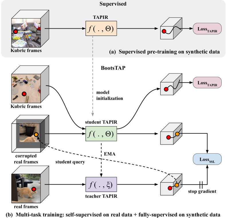
Our architecture is outlined in Figure 1. We begin with a strong “teacher” model pre-trained using supervised learning on synthetic data (in our case, a TAPIR [10] model) which serves as initialization for both a “teacher” and a “student” model. Given an unlabeled input video, we make a prediction using the teacher model, which serves as pseudo-ground-truth for the student. We then generate a second “view” of the video by applying affine transformations that vary smoothly in time, re-sampling frames to a lower resolution (while padding back to the original size), and adding JPEG corruption. We input the second view to the “student” network and use a query point sampled from the teacher’s prediction (transformed consistently with the transformation applied to the video). The student’s prediction is then transformed back into the original coordinate space. We then compute a “self-supervised loss,” which is simply TAPIR’s original loss function applied to the student predictions, using teacher’s predictions as pseudo-ground-truth. The teacher’s weights are updated by using an exponential moving average (EMA) of the student’s weights. We take steps to ensure that the teacher’s predictions used for training are more likely to be accurate than the student’s: (i) the corruptions that degrade and downsample the video are only applied to the student’s inputs, (ii) we use an EMA of the student’s weights as the teacher’s weights, which we empirically find makes the teacher’s outputs more accurate and stable, finally, (iii) we only train on points that are closer (in time) to the teacher’s query point than they are to the student’s. We show that this formulation, when applied to real-world videos (15M clips) provides a substantial boost over prior state-of-the-art across the entire TAP-Vid benchmark.
In summary, our contributions are as follows:
-
1.
We demonstrate the first large-scale pipeline for improving video point tracking using a large dataset of unannotated videos, based on straightforward properties of real trajectories: (i) predictions should vary consistently with spatial transformations of the video, and (ii) predictions should be invariant to the choice of query point along a given trajectory.
-
2.
We show that the resulting formulation achieves new SoTA results on point tracking benchmarks, while requiring minimal architectural changes.
-
3.
We release a checkpoint on GitHub, and include model implementations in both JAX and PyTorch for the community to use, available at https://github.com/google-deepmind/tapnet.
2 Related Work
Tracking-Any-Point.
The ability to track densely-sampled points over long video sequences is a generic visual capability [44, 45]. Because this visual task provides a rich output that is well-defined independent of semantic or linguisitic categories (unlike classification, detection, and semantic segmentation), it is more generically useful and can support other visual capabilities like video editing [60], 3D estimation [54], object segmentation [39, 42], and even robotics [52, 58]. Point tracking has recently experienced a flurry of recent works including new datasets [9, 63, 1] and algorithms [18, 25, 10, 54, 37]. Current state-of-the-art works mainly train in a supervised manner, relying heavily on synthetic data [16] which has a large domain gap with the real world.
Self-supervised correspondence via photometric loss.
Tracking has long been a target of self-supervised learning due to the lack of reliable supervised data, especially at the point level. A wide variety of proxy supervisory signals have been proposed, all with their own limitations. Photometric losses use reconstruction, and are particularly popular in optical flow, but occlusions, lighting changes, and repeated (or constant) textures, typically result in multiple or false appearance matches. To compensate for this, these methods typically rely on complicated priors such as multi-frame estimation [22], explicit occlusion handling [47, 57], improved data augmentation [30], additional loss terms [31, 32, 36], and robust loss functions which avoid degenerate solutions [61, 43, 34]. Methods that combine feature learning with appearance reconstruction, such as [53, 29, 28], have demonstrated long-range tracking. Matches based on local appearance are more likely to correspond to motion in high resolution videos because they are able to resolve detailed textures [23]; we make use of this observation in our work.
Temporal continuity and cycle-consistency.
Other works use images or videos to perform more general feature learning, with the aim that features in correspondence should be more similar than those which are not. Temporal continuity in videos has long been used to obtain such correspondences [12, 59, 13, 55, 21], resulting in features which have proven to be effective for object tracking [7, 14]. Temporal cycle-consistency [56, 2] can also result in features useful for tracking; however this learning method fails to provide useful supervision in challenging situations such as occlusions.
Semi-supervised correspondence.
A final self-supervised approach is to create synthetic pairs from real images where correspondences are known [19, 46]. Such approaches have a long history in optical flow [31, 32, 20, 38], although with mixed results, typically requiring complex training setups such as GANs [27] or connecting the student to the teacher [33] to prevent trivial solutions. They have only been applied to longer-term point tracking more recently [54, 48]. OmniMotion computes initial point tracks using RAFT [50] or TAP-Net [9] and infers a full pseudo-3D interpretation of the scene in the form of a neural network. Although this method improves point tracks compared to their initialization, it never retrains a general TAP model on the self-labeled data. Concurrent work [48], on the other hand, saves a dataset of point tracks and retrains the underlying model on them, using data augmentations similar to ours. Unlike our work, however, it trains only on relatively small, downstream datasets, and it does not update the underlying point tracks as the model improves. They report that performance quickly saturates and begins to degrade with more training iterations, which is a key limitation for scaling the method that our algorithm overcomes. We discuss the differences in more detail in the following section, after presenting our approach.
3 Method
When developing a self-training method for TAP, it is important to note that, like in optical flow, TAP has a precise, correct answer for the vast majority of query points. This is different from typical visual self-supervised learning, where the representation can be arbitrary, as long as semantically similar images have similar representations. Supervised learning on synthetic data provides a strong initial guess in many situations, but care must be taken to ensure that the self-supervised algorithm does not find “trivial shortcuts” [8] that become self-reinforcing and harm the initialization.
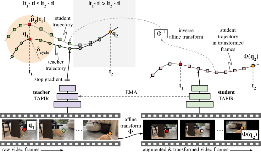
Our formulation relies on two facts about point tracks that are true for points on any solid, opaque surface. First, spatial transformations (e.g. affine transformations) which are applied to the video will result in equivalent spatial transformations of the point tracks (i.e. the tracks are “equivariant” under spatial transformation), while the tracks are invariant to many other factors of variation that do not move the image content (e.g. color changes, noise). Second, the algorithm should output the same track regardless of which point along the track is used as a query; mathematically, this means that each trajectory forms an equivalence class. One could imagine enforcing the desired equivariance and invariance properties using a simple Siamese-network formulation [17], where a single network is trained to output consistent predictions on two different ‘views’ of the data. However, we find that minimizing the difference between the two outputs—and backpropping both—results in predictions degrading toward trivial solutions (e.g. over-smoothing of tracks, or tracking the image boundary instead of the image contents). In fact, the model can learn to distinguish between synthetic and real data resulting in trivial solutions on the real, unlabeled data only. To prevent this, we adopt a student-teacher framework, where the student’s view of the data is made more challenging by augmentations, and the teacher does not receive gradients that may corrupt its predictions. Figure 2 shows the overall pipeline.
We start with a baseline TAPIR network pre-trained on Kubric in the standard way [10]. Let be the predictions: is position, is an occlusion logit, and is an uncertainty logit, where is the number of frames. Calling and the ground truth targets for frame , recall that the standard TAPIR loss for a single trajectory is defined as:
| Position loss | |||||
| Occlusion loss | (1) | ||||
| Uncertainty loss |
where Huber is the Huber loss and BCE is the sigmoid binary cross-entropy. The target for the uncertainty logit is defined as , where the distance and is a threshold on the distance, set to 6 pixels, and is an indicator function. That is, the uncertainty loss trains the model to predict whether its own prediction is likely to be within a threshold of the ground truth.
After pre-training, we add a few extra convolutional residual layers to the backbone, initialized to the identity [15], to absorb the extra training data. Let now refer to the student predictions. We derive pseudo-labels from the teacher’s predictions as follows:
| (2) |
where indexes time. The loss for a given video frame is derived from the TAPIR loss, treating the pseudo-labels as ground-truth, and defined as:
| (3) | ||||
Note that TAPIR’s loss uses multiple refinement iterations, but we always use the teacher’s final prediction to derive pseudo-ground-truth; therefore, refined predictions serve as supervision for unrefined ones, encouraging stronger features that enable faster convergence.
While the above formulation is well-defined, if the student and teacher both receive the same video and query point, we expect the loss to be trivially close to zero, so we apply transformations and corruptions to the student’s view. Given an input video, we create a second view by resizing each frame to a smaller resolution (varying linearly over time) and superimposing them onto a black background at a random position (also varying linearly across time); formally, this is a frame-wise axis-aligned affine transformation on coordinates, applied to the pixels. We also apply to the student query coordinates. We further degrade this view by applying a random JPEG degradation to make the task more difficult, before pasting it onto the black background. Both operations lose texture information; therefore, the network must learn higher-level—and possibly semantic—cues (e.g. the tip of the top left ear of the cat), rather than lower-level texture matching in order to track points correctly. We apply the inverse affine transformation to map the student’s predictions back to the original input coordinate space, before feeding these to the loss. We describe these transformations and corruptions in more detail in Appendix 0.B.1.
Second, we enforce that each track forms an equivalence class by training the model to produce the same track regardless of which point is used as a query. While we do not have access to the ground-truth trajectories to sample different query points from, we can use the teacher model’s predictions to form pairs of query points. First, we sample a query point , where is an coordinate, and is a frame index, both sampled uniformly. Then the student’s query is sampled randomly from the teacher’s trajectory, i.e. .
Note, however, that if the teacher has not tracked the point correctly, the student’s query might be a different real-world point than the teacher’s, leading to an erroneous training signal. To prevent this, we use cycle-consistency of the student and teacher trajectories, and ignore the loss for trajectories that don’t form a valid cycle, as depicted by the orange circle in Figure 2. Formally, we implement this as a mask defined as:
| (4) |
Here, is a distance threshold hyperparameter, which we set to 4 pixels. Furthermore, we expect that the teacher’s predictions may be less accurate than the student’s for points that are closer in time to the student’s query frame than they are to the teacher’s. Therefore, we filter these points, as depicted by the grey squares/circles in Figure 2. We define a second mask as follows:
| (5) |
Note that there is a special case when the student and teacher have the same query point: there is no longer any uncertainty regarding whether the point is on the same trajectory. These points are reliable while also being less challenging. We compromise between extremes, and have half the time (and set the masks to 1’s), and the rest of the time sample uniformly from the visible points in the teacher prediction. The final self-supervised loss for a single trajectory is then:
| (6) |
In practice, we sample 128 query points per input video and average the loss for all of them. For a recap of the algorithm, see Appendix 0.A.
To avoid catastrophic forgetting, we continue training on the Kubric dataset with the regular supervised TAPIR loss. Our training setup follows prior work on multi-task self-supervised learning [11]: we maintain separate Adam optimizer parameters to compute separate updates for both tasks, and then apply the gradients with their own learning rates. As the self-supervised task is more expensive due to the extra forward pass, we use half the batch size for self-supervised updates, and therefore we halve the learning rate for these updates. See Appendix 0.B.2
Note that concurrent work [48] reproduces some of these decisions, including using cycle-consistency as a method of filtering the pseudo-ground-truth and using similar augmentations before passing to the student model, e.g. affine transformations. They have a filtering step based on cycle-consistency similar to , but do not filter based on proximity like . Rather than a student-teacher setup, they compute trajectories only once and freeze the training data, meaning that the model is permanently trained to reproduce errors in the original labeling. Furthermore, the work fine-tunes on the target dataset, meaning that new domains require a potentially large training set and a re-start of the fine-tuning; in contrast, our work demonstrates that it’s possible to train on a single large dataset that covers many domains, meaning that fine-tuning is unnecessary.
4 Experiments
We train our model on over 15 million 24-frame clips from from publicly-available online videos, in conjunction with standard training on Kubric. The resulting model is essentially a drop-in replacement for TAPIR (albeit with slightly larger computational requirements due to the extra layers). We evaluate on the TAP-Vid benchmark using the standard protocol.
4.1 Training datasets
We collected a video dataset from publicly accessible videos selected from categories that typically contain high-quality and realistic motion (such as lifestyle and one-shot videos). Conversely, we omitted videos from categories with low visual complexity or unrealistic motions, such as tutorial videos, lyrics videos, and animations. To maintain consistency, we exclusively obtained videos with shot at 60fps. Additionally, we applied a quality metric by only considering videos with over 200 views. We removed the first and last 2 seconds of each video, as these often contain intros and outros with text or other overlays. From each video, we randomly sampled five clips, excluding those with overlay/watermarked frames, which were identified by checking the horizontal and vertical gradients and computing the pixel-wise median (similar to [6]). Furthermore, we expect the teacher signal will be more reliable on continuous shots due to temporal continuity; therefore, clips with shot boundary changes are detected and removed based on [3, 62, 51, 35] with additional accuracy improvements based on full-frame geometric alignment. In total, we generated 15 million clips for training.
4.2 Evaluation datasets
We rely on the TAP-Vid [9] and RoboTAP [52] benchmarks for quantitative evaluation; in all cases, we evaluate zero-shot on the entire benchmark, resizing to before evaluating according to the standard procedure [9]. All evaluation datasets consists of real world videos.
TAP-Vid-Kinetics contains videos collected from the Kinetics-700-2020 validation set [5] with original focus on video action recognition. This benchmark contains 1K YouTube videos of diverse action categories, approximately 10 seconds long, including many challenging elements such as shot boundaries, multiple moving objects, dynamic camera motion, cluttered background and dark lighting conditions. Each video contains 26 tracked points on average, obtained from careful human annotation.
TAP-Vid-DAVIS contains 30 real-world videos from DAVIS 2017 validation set [41], a standard benchmark for video object segmentation, which was extended to TAP. Each video contains 22 point tracks using the same human annotation process as TAP-Vid-Kinetics.
RoboTAP contains 265 real world Robotics Manipulation videos with on average 272 frames and 44 annotated point tracks per video [52]. These videos are even longer, with textureless and symmetric objects that are far out-of-domain for both Kubric and the online lifestyle videos that we use for self-supervised learning.
RoboCAT-NIST is a subset of the data collected for RoboCat [4]. Inspired by the NIST benchmark for robotic manipulation [26], it includes gears of varying sizes (small, medium, large) and a 3-peg base, introduced for a systematic study of insertion affordance. All videos are collected by human teleoperation. It includes 100,000 real world videos with different robot arms operating and inserting gears, which are a particularly challenging case due to the rotational symmetry and lack of texture. In this work, we processed videos to 64 frames long with 222x296 resolution. This dataset is mainly for demonstration purpose, there are no human groundtruth point tracks.
4.3 Evaluation metrics
We use three evaluation metrics same as proposed in [9]. (1) is the average position accuracy across 5 thresholds for : 1, 2, 4, 8, 16 pixels. For a given threshold , it computes the proportion of visible points (not occluded) that are closer to the ground truth than the respective threshold. (2) Occlusion Accuracy (OA) is the average binary classification accuracy for the point occlusion prediction at each frame. (3) Average Jaccard (AJ) combines the two above metrics and is typically considered the target for this benchmark. It is the average Jaccard score across the same thresholds as . Jaccard at measures both occlusion and position accuracy. It is the fraction of ‘true positives’, i.e., points within the threshold of any visible ground truth points, divided by ‘true positives’ plus ‘false positives’ (points that are predicted visible, but the ground truth is either occluded or farther than the threshold) plus ‘false negatives’ (groundtruth visible points that are predicted as occluded, or where the prediction is farther than the threshold).
For TAP-Vid datasets, evaluation is split into strided mode and first mode. Strided mode samples query points every 5 frames on the groundtruth tracks when they are visible. Query points can be any time in the video hence it tests the model prediction power both forward and backward in time. First mode samples query points only when they are first time visible and the evaluation only measures tracking accuracy in future frames.
4.4 Results
| Kinetics | DAVIS | RGB-Stacking | |||||||
|---|---|---|---|---|---|---|---|---|---|
| Method | AJ | OA | AJ | OA | AJ | OA | |||
| COTR [24] | 19.0 | 38.8 | 57.4 | 35.4 | 51.3 | 80.2 | 6.8 | 13.5 | 79.1 |
| Kubric-VFS-Like [16] | 40.5 | 59.0 | 80.0 | 33.1 | 48.5 | 79.4 | 57.9 | 72.6 | 91.9 |
| RAFT [50] | 34.5 | 52.5 | 79.7 | 30.0 | 46.3 | 79.6 | 44.0 | 58.6 | 90.4 |
| PIPs [18] | 35.3 | 54.8 | 77.4 | 42.0 | 59.4 | 82.1 | 37.3 | 51.0 | 91.6 |
| TAP-Net [9] | 46.6 | 60.9 | 85.0 | 38.4 | 53.1 | 82.3 | 59.9 | 72.8 | 90.4 |
| TAPIR [10] | 57.2 | 70.1 | 87.8 | 61.3 | 73.6 | 88.8 | 62.7 | 74.6 | 91.6 |
| CoTracker [25] | - | - | - | 64.8 | 79.1 | 88.7 | - | - | - |
| BootsTAPIR | 61.5 | 74.2 | 89.7 | 66.4 | 78.5 | 90.7 | 73.4 | 83.2 | 92.3 |
Our results are shown in Table 1. Note that all of our numbers come from a single checkpoint, which has not seen the relevant datasets. Relative to our base architecture, our bootstrapping approach provides a substantial gain across all metrics. We also outperform CoTracker on DAVIS, though this is due more to improvements in occlusion accuracy than position accuracy. This is despite TAPIR having a simpler architecture than CoTracker, which requires cross attention to other points which must be chosen with a hand-tuned distribution, whereas TAPIR tracks points independently. CoTracker results are also obtained by upsampling videos to , which further increases compute time, whereas ours are computed directly on videos.
| Kinetics | DAVIS | RoboTAP | |||||||
|---|---|---|---|---|---|---|---|---|---|
| Method | AJ | OA | AJ | OA | AJ | OA | |||
| TAP-Net [9] | 38.5 | 54.4 | 80.6 | 33.0 | 48.6 | 78.8 | 45.1 | 62.1 | 82.9 |
| TAPIR [10] | 49.6 | 64.2 | 85.0 | 56.2 | 70.0 | 86.5 | 59.6 | 73.4 | 87.0 |
| CoTracker [25] | 48.7 | 64.3 | 86.5 | 60.6 | 75.4 | 89.3 | - | - | - |
| BootsTAPIR | 54.7 | 68.5 | 86.3 | 61.4 | 74.0 | 88.4 | 69.9 | 80.9 | 91.9 |
Table 2 shows performance under “first” metrics. Here, we see that bootstrapping outperforms prior works by a wide margin on Kinetics; this is likely because TAPIR’s global search is more robust to large occlusions and cuts, which are more prominent in Kinetics. This search might harm performance in datasets like DAVIS with a stronger temporal continuity bias. Perhaps most surprising is the very strong improvement in RoboTAP–almost 10% absolute performance–despite RoboTAP looking very different from typical online videos. We see similar results for RGB-Stacking in 1. These two datasets have large textureless regions; such regions are challenging to track without priors for object segmentation, which are difficult to obtain from synthetic datasets.
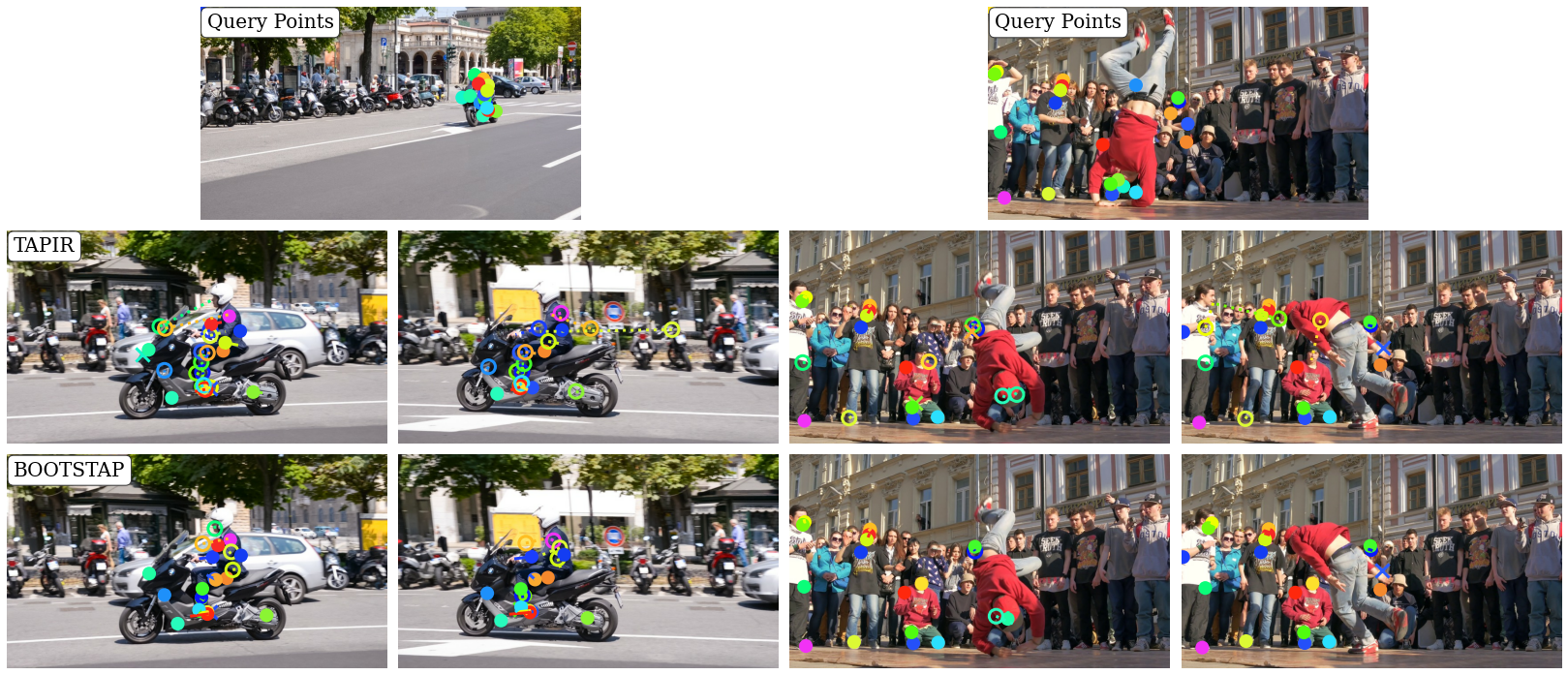
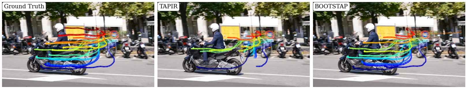
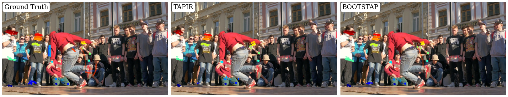
Figure 3 shows two representative examples where BootsTAP improves TAPIR on TAP-Vid-DAVIS. We notice that the main improvements come from occlusion prediction and precise localization. The scooter example clearly shows BootsTAP outperforms on occlusion estimation, but also note that for some of the points TAPIR incorrectly marks as occluded, the localization estimate is also quite bad (the green and yellow points, predicted to be on background). In the breakdance example, we see that TAPIR marks several background points as occluded despite very little motion, likely due to the large number of people (note Kubric contains no humans). The improved occlusion accuracy here suggests that the model has learned about distinguishing different people from its experience with real videos.


Figure 4 shows more examples for where BootsTAP improves TAPIR on RoboTAP dataset. We show the groundtruth tracks, TAPIR prediction and BootsTAP prediction, where each trajectory is plotted over the last video frame with a different color. Even though RoboTAP contains different views, we select mainly the wrist camera views as examples where the improvements from BootsTAP are particularly clear. TAPIR loses many points due to the large motion and lack of texture, but BootsTAP recovers them.
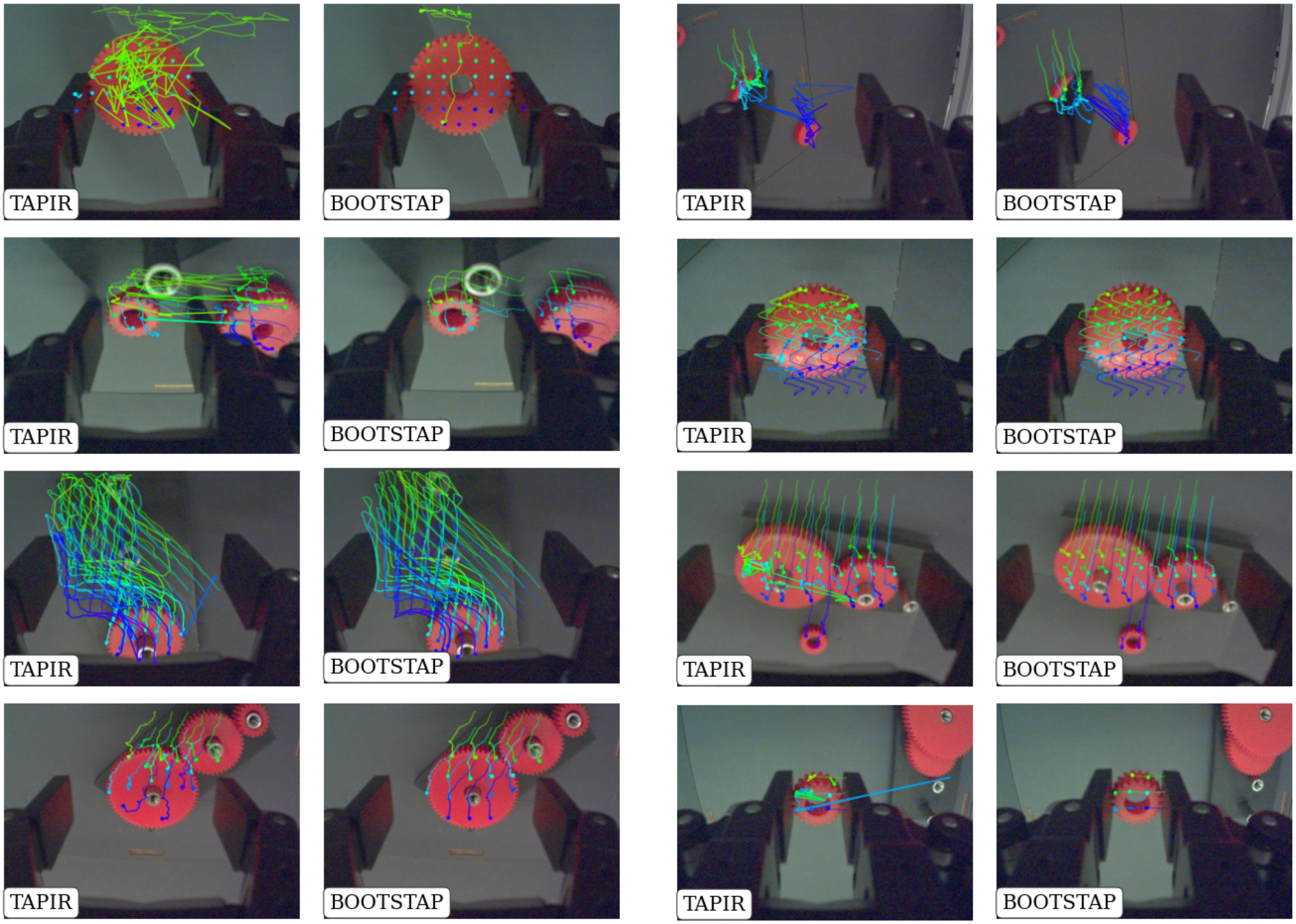
Figure 5 further illustrates improvements on the RoboCAT-NIST dataset, using a model where 100K RoboCAT-NIST clips were added to the online data. Due to the lack of groundtruth, we instead sample a grid of points on the gears (i.e. red pixels). We display a few examples comparing the predicted tracks between the two models. As these are rigid objects, we expect the points to move consistently within each gear; deviations from this are errors. Due to the lack of texture on the gears and the nontrivial sim2real transfer gap, the original TAPIR trained on Kubric works poorly here, with many jittery tracks and severe tracking failures. This is particularly bad for points that are close to occlusion or out of image boundary. The bootstrapped model fixes many of these failures: the tracks are much smoother and occlusion predictions become much more accurate.
5 Conclusion
In this work we presented an effective method for leveraging large scale, unlabeled data for improving TAP performance. We have demonstrated that a straightforward application of consistency principles, namely invariance to query points and non-spatial corruptions, and equivariance to affine transformations, enable the model to continue to improve on unlabeled data. Our formulation avoids more complex priors such as spatial smoothness of motion or temporal smoothness of tracks that are used in many prior works. In fact, our formulation bears similarities to baselines for two-frame, self-supervised optical flow that are considered too “unstable” to be effective (c.f. Fig. 2(a) in “Flow Supervisor” [20]). Yet in our multi-frame approach, we ultimately surpass the state-of-the-art performance by a large margin. We find little evidence of model ‘overfitting’ to its own biases in ways that cause performance to degrade with long training like in other work [48]. Instead, we find that performance continues to improve for as long as we train the model. Our work does have some limitations: training remains computationally expensive. Furthermore, our estimated correspondence is a single point estimate throughout the entire video, which means we cannot elegantly handle duplicated or rotationally-symmetric objects where the actual correspondence is ambiguous. Nevertheless, our approach demonstrates that it is possible to better bridge the sim-to-real gap using self-supervised learning.
Acknowledgements
. We thank Ignacio Rocco, Yusuf Aytar, David Fleet, Daniel Zoran, Jon Scholz, and Nando de Freitas for helpful conversations and advice. We thank Lucas Smaira, Ed Hirst, Alexandre Moufarek, Jack Parker-Holder and Junlin Zhang for help with dataset construction.
References
- [1] Balasingam, A., Chandler, J., Li, C., Zhang, Z., Balakrishnan, H.: Drivetrack: A benchmark for long-range point tracking in real-world videos. arXiv preprint arXiv:2312.09523 (2023)
- [2] Bian, Z., Jabri, A., Efros, A.A., Owens, A.: Learning pixel trajectories with multiscale contrastive random walks. In: Proc. CVPR (2022)
- [3] Boreczky, J.S., Rowe, L.A.: Comparison of video shot boundary detection techniques. Journal of Electronic Imaging 5(2), 122–128 (1996)
- [4] Bousmalis, K., Vezzani, G., Rao, D., Devin, C., Lee, A.X., Bauza, M., Davchev, T., Zhou, Y., Gupta, A., Raju, A., et al.: Robocat: A self-improving foundation agent for robotic manipulation. arXiv preprint arXiv:2306.11706 (2023)
- [5] Carreira, J., Zisserman, A.: Quo vadis, action recognition? a new model and the kinetics dataset. In: Proc. CVPR. pp. 6299–6308 (2017)
- [6] Dekel, T., Rubinstein, M., Liu, C., Freeman, W.T.: On the effectiveness of visible watermarks. In: Proc. CVPR (2017)
- [7] Denil, M., Bazzani, L., Larochelle, H., de Freitas, N.: Learning where to attend with deep architectures for image tracking. Neural computation 24(8), 2151–2184 (2012)
- [8] Doersch, C., Gupta, A., Efros, A.A.: Unsupervised visual representation learning by context prediction. In: Proc. ICCV (2015)
- [9] Doersch, C., Gupta, A., Markeeva, L., Recasens, A., Smaira, L., Aytar, Y., Carreira, J., Zisserman, A., Yang, Y.: TAP-Vid: A benchmark for tracking any point in a video. NeurIPS (2022)
- [10] Doersch, C., Yang, Y., Vecerik, M., Gokay, D., Gupta, A., Aytar, Y., Carreira, J., Zisserman, A.: TAPIR: Tracking any point with per-frame initialization and temporal refinement. arXiv preprint arXiv:2306.08637 (2023)
- [11] Doersch, C., Zisserman, A.: Multi-task self-supervised visual learning. In: Proc. ICCV (2017)
- [12] Földiák, P.: Learning invariance from transformation sequences. Neural computation 3(2), 194–200 (1991)
- [13] Goroshin, R., Bruna, J., Tompson, J., Eigen, D., LeCun, Y.: Unsupervised learning of spatiotemporally coherent metrics. In: Proc. ICCV (2015)
- [14] Goroshin, R., Mathieu, M.F., LeCun, Y.: Learning to linearize under uncertainty. NeurIPS (2015)
- [15] Goyal, P., Dollár, P., Girshick, R., Noordhuis, P., Wesolowski, L., Kyrola, A., Tulloch, A., Jia, Y., He, K.: Accurate, large minibatch SGD: Training imagenet in 1 hour. arXiv preprint arXiv:1706.02677 (2017)
- [16] Greff, K., Belletti, F., Beyer, L., Doersch, C., Du, Y., Duckworth, D., Fleet, D.J., Gnanapragasam, D., Golemo, F., Herrmann, C., et al.: Kubric: A scalable dataset generator. In: Proc. CVPR (2022)
- [17] Hadsell, R., Chopra, S., LeCun, Y.: Dimensionality reduction by learning an invariant mapping. In: Proc. CVPR (2006)
- [18] Harley, A.W., Fang, Z., Fragkiadaki, K.: Particle video revisited: Tracking through occlusions using point trajectories. In: Proc. ECCV (2022)
- [19] Huang, H.P., Herrmann, C., Hur, J., Lu, E., Sargent, K., Stone, A., Yang, M.H., Sun, D.: Self-supervised autoflow. In: Proc. CVPR (2023)
- [20] Im, W., Lee, S., Yoon, S.E.: Semi-supervised learning of optical flow by flow supervisor. In: Proc. ECCV (2022)
- [21] Jabri, A., Owens, A., Efros, A.: Space-time correspondence as a contrastive random walk. NeurIPS 33, 19545–19560 (2020)
- [22] Janai, J., Guney, F., Ranjan, A., Black, M., Geiger, A.: Unsupervised learning of multi-frame optical flow with occlusions. In: Proc. ECCV (2018)
- [23] Janai, J., Guney, F., Wulff, J., Black, M.J., Geiger, A.: Slow flow: Exploiting high-speed cameras for accurate and diverse optical flow reference data. In: Proc. CVPR (2017)
- [24] Jiang, W., Trulls, E., Hosang, J., Tagliasacchi, A., Yi, K.M.: COTR: Correspondence transformer for matching across images. In: Proc. ICCV (2021)
- [25] Karaev, N., Rocco, I., Graham, B., Neverova, N., Vedaldi, A., Rupprecht, C.: CoTracker: It is better to track together. arXiv preprint arXiv:2307.07635 (2023)
- [26] Kimble, K., Van Wyk, K., Falco, J., Messina, E., Sun, Y., Shibata, M., Uemura, W., Yokokohji, Y.: Benchmarking protocols for evaluating small parts robotic assembly systems. Proc. Intl. Conf. on Robotics and Automation 5(2), 883–889 (2020)
- [27] Lai, W.S., Huang, J.B., Yang, M.H.: Semi-supervised learning for optical flow with generative adversarial networks (2017)
- [28] Lai, Z., Lu, E., Xie, W.: MAST: A memory-augmented self-supervised tracker. In: Proc. CVPR (2020)
- [29] Lai, Z., Xie, W.: Self-supervised learning for video correspondence flow. arXiv preprint arXiv:1905.00875 (2019)
- [30] Liu, L., Zhang, J., He, R., Liu, Y., Wang, Y., Tai, Y., Luo, D., Wang, C., Li, J., Huang, F.: Learning by analogy: Reliable supervision from transformations for unsupervised optical flow estimation. In: Proc. CVPR (2020)
- [31] Liu, P., King, I., Lyu, M.R., Xu, J.: Ddflow: Learning optical flow with unlabeled data distillation. In: Proceedings of the AAAI conference on artificial intelligence. vol. 33, pp. 8770–8777 (2019)
- [32] Liu, P., Lyu, M., King, I., Xu, J.: Selflow: Self-supervised learning of optical flow. In: Proc. CVPR (2019)
- [33] Liu, P., Lyu, M.R., King, I., Xu, J.: Learning by distillation: a self-supervised learning framework for optical flow estimation. IEEE PAMI 44(9), 5026–5041 (2021)
- [34] Marsal, R., Chabot, F., Loesch, A., Sahbi, H.: Brightflow: Brightness-change-aware unsupervised learning of optical flow. In: Proc. WACV (2023)
- [35] Mas, J., Fernandez, G.: Video shot boundary detection based on color histogram. In: TRECVID (2003)
- [36] Meister, S., Hur, J., Roth, S.: Unflow: Unsupervised learning of optical flow with a bidirectional census loss. In: Proceedings of the AAAI conference on artificial intelligence. vol. 32 (2018)
- [37] Neoral, M., Šerỳch, J., Matas, J.: Mft: Long-term tracking of every pixel. In: Proc. WACV (2024)
- [38] Novák, T., Šochman, J., Matas, J.: A new semi-supervised method improving optical flow on distant domains. In: Computer Vision Winter Workshop. vol. 3 (2020)
- [39] Ochs, P., Malik, J., Brox, T.: Segmentation of moving objects by long term video analysis. IEEE transactions on pattern analysis and machine intelligence 36(6), 1187–1200 (2013)
- [40] OpenAI: Gpt-4v(ision) system card (September 25, 2023)
- [41] Perazzi, F., Pont-Tuset, J., McWilliams, B., Van Gool, L., Gross, M., Sorkine-Hornung, A.: A benchmark dataset and evaluation methodology for video object segmentation. In: Proc. CVPR (2016)
- [42] Rajič, F., Ke, L., Tai, Y.W., Tang, C.K., Danelljan, M., Yu, F.: Segment anything meets point tracking. arXiv preprint arXiv:2307.01197 (2023)
- [43] Ren, Z., Yan, J., Ni, B., Liu, B., Yang, X., Zha, H.: Unsupervised deep learning for optical flow estimation. In: Proceedings of the AAAI conference on artificial intelligence. vol. 31 (2017)
- [44] Rubinstein, M., Liu, C., Freeman, W.T.: Towards longer long-range motion trajectories. In: Proc. BMVC (2012)
- [45] Sand, P., Teller, S.: Particle video: Long-range motion estimation using point trajectories. Proc. ICCV (2008)
- [46] Shen, Y., Hui, L., Xie, J., Yang, J.: Self-supervised 3d scene flow estimation guided by superpoints. In: Proc. CVPR (2023)
- [47] Stone, A., Maurer, D., Ayvaci, A., Angelova, A., Jonschkowski, R.: Smurf: Self-teaching multi-frame unsupervised raft with full-image warping. In: Proc. CVPR (2021)
- [48] Sun, X., Harley, A.W., Guibas, L.J.: Refining pre-trained motion models. arXiv preprint arXiv:2401.00850 (2024)
- [49] Team, G., Anil, R., Borgeaud, S., Wu, Y., Alayrac, J.B., Yu, J., Soricut, R., Schalkwyk, J., Dai, A.M., Hauth, A., et al.: Gemini: a family of highly capable multimodal models. arXiv preprint arXiv:2312.11805 (2023)
- [50] Teed, Z., Deng, J.: RAFT: Recurrent all-pairs field transforms for optical flow. In: Proc. ECCV (2020)
- [51] Truong, B.T., Dorai, C., Venkatesh, S.: New enhancements to cut, fade, and dissolve detection processes in video segmentation. In: Proceedings of the eighth ACM international conference on Multimedia. pp. 219–227 (2000)
- [52] Vecerik, M., Doersch, C., Yang, Y., Davchev, T., Aytar, Y., Zhou, G., Hadsell, R., Agapito, L., Scholz, J.: RoboTAP: Tracking arbitrary points for few-shot visual imitation. In: Proc. Intl. Conf. on Robotics and Automation (2024)
- [53] Vondrick, C., Shrivastava, A., Fathi, A., Guadarrama, S., Murphy, K.: Tracking emerges by colorizing videos. In: Proc. ECCV (2018)
- [54] Wang, Q., Chang, Y.Y., Cai, R., Li, Z., Hariharan, B., Holynski, A., Snavely, N.: Tracking everything everywhere all at once. In: Proc. ICCV (2023)
- [55] Wang, X., Gupta, A.: Unsupervised learning of visual representations using videos. In: Proc. ICCV (2015)
- [56] Wang, X., Jabri, A., Efros, A.A.: Learning correspondence from the cycle-consistency of time. In: Proc. CVPR (2019)
- [57] Wang, Y., Yang, Y., Yang, Z., Zhao, L., Wang, P., Xu, W.: Occlusion aware unsupervised learning of optical flow. In: Proc. CVPR (2018)
- [58] Wen, C., Lin, X., So, J., Chen, K., Dou, Q., Gao, Y., Abbeel, P.: Any-point trajectory modeling for policy learning. arXiv preprint arXiv:2401.00025 (2023)
- [59] Wiskott, L., Sejnowski, T.J.: Slow feature analysis: Unsupervised learning of invariances. Neural computation 14(4), 715–770 (2002)
- [60] Yu, E., Blackburn-Matzen, K., Nguyen, C., Wang, O., Habib Kazi, R., Bousseau, A.: Videodoodles: Hand-drawn animations on videos with scene-aware canvases. ACM Transactions on Graphics 42(4), 1–12 (2023)
- [61] Yu, J.J., Harley, A.W., Derpanis, K.G.: Back to basics: Unsupervised learning of optical flow via brightness constancy and motion smoothness. In: Computer Vision–ECCV 2016 Workshops: Amsterdam, The Netherlands, October 8-10 and 15-16, 2016, Proceedings, Part III 14 (2016)
- [62] Yusoff, Y., Christmas, W.J., Kittler, J.: Video shot cut detection using adaptive thresholding. In: Proc. BMVC (2000)
- [63] Zheng, Y., Harley, A.W., Shen, B., Wetzstein, G., Guibas, L.J.: PointOdyssey: A large-scale synthetic dataset for long-term point tracking. In: Proc. CVPR (2023)
Appendix 0.A Summary of the approach
We summarize notations and computation of our self-supervised loss in Algorithm 1.
refers to the uniform distribution over domain ;
we denote queries as where is x/y coordinates and is a frame index. In a slight abuse of notation, we call the transformation and the mapping that transforms coordinates and leaves other model outputs unchanged.
Appendix 0.B Implementation details
0.B.1 Distribution over affine transformation
To enforce equivariance to spatial transformations, for the frames and query point coordinates, we apply a frame-wise affine transformation , whose scaling parameters and translation parameters vary linearly over time, randomly sampled from a distribution that we describe next.
We first sample a pair of initial and final spatial dimensions and from a distribution defined as follows. For each pair, we first sample an area uniformly over . Next we sample values and derive random height value by averaging them and width value ; and finally, we multiply these values by the input’s original shape . This gives us a pair of spatial dimensions biased towards aspect ratios close to 1, and covering an area between and of the original input.
We also sample a pair of initial spatial coordinates for the top-left corner of the transformed view, within the frame, uniformly over , where and respectively correspond to the maximum amount of vertical and horizontal padding that can be added to the top and left of the rescaled view. We proceed analogously to sample a pair of final spatial coordinates , given .
Let be a frame index. Calling , we then linearly interpolate between these four pairs of values; we define:
| (7) | |||
| (8) | |||
| (9) | |||
| (10) |
Finally, we apply the following transformation to the query point coordinates:
| (11) |
Given an input frame , the corresponding transformation is applied with:
| (12) |
where consists in scaling its input frame to resolution using bilinear interpolation and placing it within a zero-valued array of shape such that its top-left corner in the array is at coordinates . We note that in our approach, this transformation is performed after augmenting each frame, i.e. on .
0.B.2 Training details
We train for 200,000 iterations on 256 nVidia A100 GPUs, with a batch size of 4 Kubric videos and 2 real videos per device. The extra layers consist of 5 residual blocks on top of the backbone (which has stride 8, 256 channels), each of which consists of 2 sequential convolutions with a channel expansion factor of 4, which is then added to the input. We use a cosine learning rate schedule with 1000 warmup steps and a peak learning rate of 2e-4. We found it improved stability to reduce the learning rate for the PIPs mixer steps relative to the backbone by a factor of 5. We keep all other hyperparameters the same as TAPIR.