Intrinsic Data Constraints and Upper Bounds in Binary Classification Performance

Abstract

The structure of data organization is widely recognized as having a substantial influence on the efficacy of machine learning algorithms, particularly in binary classification tasks. Our research provides a theoretical framework suggesting that the maximum potential of binary classifiers on a given dataset is primarily constrained by the inherent qualities of the data. Through both theoretical reasoning and empirical examination, we employed standard objective functions, evaluative metrics, and binary classifiers to arrive at two principal conclusions. Firstly, we show that the theoretical upper bound of binary classification performance on actual datasets can be theoretically attained. This upper boundary represents a calculable equilibrium between the learning loss and the metric of evaluation. Secondly, we have computed the precise upper bounds for three commonly used evaluation metrics, uncovering a fundamental uniformity with our overarching thesis: the upper bound is intricately linked to the dataset’s characteristics, independent of the classifier in use. Additionally, our subsequent analysis uncovers a detailed relationship between the upper limit of performance and the level of class overlap within the binary classification data. This relationship is instrumental for pinpointing the most effective feature subsets for use in feature engineering.

Machine learning research has predominantly concentrated on enhancing model accuracy, yet the predictability of machine learning problems remains insufficiently understood Hastie et al. (2009); Agresti (2012); Noble (2006); Chen and Guestrin (2016). A thorough quantification of predictability is paramount for the thoughtful design, training, and deployment of machine learning models, shedding light on the capabilities and limitations of AI in practical scenarios.

Conventional machine learning has often favored error-based metrics as objective functions. However, these metrics have proven to have a negligible impact on optimization outcomes Rosasco et al. (2004) and are prone to complications arising from imbalanced datasets in classification challenges Cortes and Mohri (2003). This recognition has sparked a surge in research directed at AUC maximization within classification tasks Yang and Ying (2022), spawning a variety of learning frameworks Joachims (2005), methodologies Ying et al. (2016), optimization techniques Norton and Uryasev (2019), and their successful implementation in a myriad of fields Yuan et al. (2021). Theoretical insights have also been advanced regarding consistency Gao and Zhou (2012) and bounding generalization errors Lei et al. (2020).

Although research has made strides in optimizing binary classifiers and demonstrating that an optimal classifier produces a convex ROC curve Fawcett (2006), the maximal AUC remains undisclosed. While efforts to probe link predictability using methods such as information entropy Sun et al. (2020) and random turbulence Lü et al. (2015) are notable, their reliance on stringent assumptions limits their applicability to extensive, real-world datasets. A gap persists in analytically defining the general predictability of machine learning in practical applications.

This paper seeks to fill this void by theoretically establishing the upper bounds for the receiver operating characteristic (ROC) curve, the precision-recall (PR) curve, and accuracy—a commonly used performance metric. Binary classification, a fundamental machine learning task that segregates entities into two distinct categories, serves as our focus due to its broad applicability. Our goal is to discern a quantifiable link between data’s intrinsic patterns and the ultimate efficacy of binary classifiers—a connection that has remained obscure Majnik and Bosnić (2013); Fawcett (2006); Metz (1978). We approach the problem by equating the determination of binary classification’s upper bound to solving a classic 0-1 knapsack problem via a greedy algorithm. The derived ROC curve thereby adheres to the optimal ROC convex hull concept as discussed in Fawcett (2001). Similar methodologies are applied to ascertain the optimal PR curve and accuracy through enumeration.

Our investigation extends to the robustness of our proposed methods under the complementarity principle Bohr et al. (1928), a concept drawing from the Pauli exclusion principle. We illustrate analytically that the divergence between training and testing datasets significantly impacts binary classifiers’ performance. Experiments with four real-world datasets corroborate the practicality and extendibility of our methods in deducing the performance upper bounds of binary classifiers.

Our analysis further identifies a direct correlation between the overlap of positive and negative instances and the performance ceiling of a dataset. Specifically, reduced overlap translates to augmented predictive capacity and likely enhanced model performance. Conversely, when positive and negative instances are indistinguishable, model efficacy is tantamount to random chance. In feature engineering, we observe that incorporating novel features (feature selection) can mitigate this overlap, thereby elevating the dataset’s performance potential. In contrast, manipulations using existing features, like feature extraction, do not affect the overlap or the upper limits of evaluation metrics.

Results
Preliminaries.
Consider a binary dataset $\mathcal{S}=\{(x_{i},y_{i})\mid i=1,2,\ldots,m\}$, where each instance consists of a $k$-dimensional feature vector $x_{i}=(x_{i,1},x_{i,2},\ldots,x_{i,k})\in\mathcal{X}$ and a corresponding class label $y_{i}\in{1,-1}$. We denote $\mathcal{X}$ as the domain comprising all unique feature vectors in $\mathcal{S}$. For a given feature vector $x_{i}$, $\mathcal{P}(x_{i})$ and $\mathcal{N}(x_{i})$ indicate the count of positive and negative samples, respectively. Additionally, the entire dataset contains $n_{+}$ positive and $n_{-}$ negative samples. The proportion of positive instances for a particular feature vector $x_{i}$ is expressed as $p_{+}(x_{i})=\mathcal{P}(x_{i})/(\mathcal{P}(x_{i})+\mathcal{N}(x_{i}))$.

Binary classification models function by assigning a feature vector $x_{i}$ to a binary class. These models are broadly categorized into two types: continuous and discrete classifiers. Continuous classifiers employ a real-valued function $f:\mathcal{X}\rightarrow\mathbb{R}$ to gauge the likelihood of an instance belonging to each class, based on a predefined threshold $t$. Examples of continuous classifiers include logistic regression Menard (2002); Hosmer Jr et al. (2013) and neural networks Haykin (1998); Albawi et al. (2017). On the other hand, discrete classifiers directly generate binary outcomes, such as support vector machines (SVM) Noble (2006); Brown et al. (2000) and decision treesKingsford and Salzberg (2008); Safavian and Landgrebe (1991).

Boundary of Evaluation Measures.
To assess the performance of binary classifiers, we investigate three prominent evaluation metrics: the ROC curve, the PR curve, and accuracy. Each of these metrics evaluates classifier performance from distinct perspectives.

Upper Bound of ROC Curve. The ROC curve is a fundamental tool for displaying the discriminative capacity of a binary classifier across various threshold settings Fawcett (2006); Metz (1978). It delineates the trade-off between sensitivity (true positive rate) and specificity (true negative rate), assisting in the selection of an optimal threshold. The area under the ROC curve (AUC-ROC) quantifies the probability that a randomly chosen positive instance is ranked higher than a negative instance, serving as a summary measure of classifier performance across all thresholds Hanley and McNeil (1982); Bradley (1997). We have established the exact upper bound of the AUC ($AR^{u}$) for a given binary dataset $\mathcal{S}$, expressed as (refer to SI Appendix, Optimal ROC Curve for the detailed mathematical derivation):

$$\text{AR}^{u}=\frac{1}{2n_{+}n_{-}}\sum\limits_{x_{i},x_{j}}\max\Big{\{}\mathcal{P}(x_{i})\mathcal{N}(x_{j}),\mathcal{P}(x_{j})\mathcal{N}(x_{i})\Big{\}},$$ (1)

where $x_{i}$ and $x_{j}$ are two arbitrary feature vectors from $\mathcal{S}$. This upper bound is attainable by a binary classifier if and only if it satisfies $f^{*}_{\text{AR}}(x_{i})\sim p_{+}(x_{i})$, where $f(x_{i})\sim f^{\prime}(x_{i})$ denotes that $f(x_{i})>f(x_{j})$ if and only if $f^{\prime}(x_{i})>f^{\prime}(x_{j})$ for every pair $(x_{i},x_{j})$ in $\mathcal{S}$.

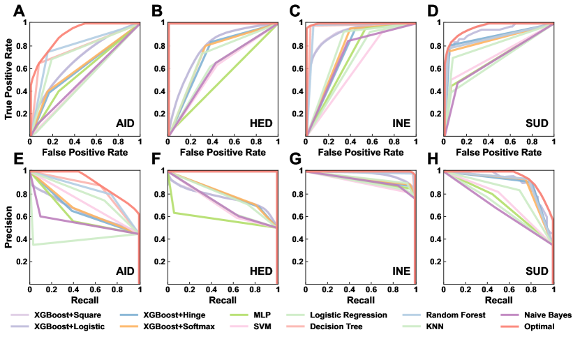
Fig. 1: Demonstrating the precise upper Bound of AUC with accompanying optimal ROC curves (A-D) and PR curves (E-H) across four real-world datasets utilizing a suite of binary classifiers. The classifiers include XGBoost, MLP, SVM, Logistic Regression, Decision Tree, Random Forest, KNN, and Naive Bayes. The red curves symbolize the theoretical optimal PR curves. Detailed values for each classifier-dataset combination are documented in Table 1.

Figure 1A-1D depicts the results of in-sample experiments featuring a suite of well-known binary classifiers, including XGBoost, Multilayer Perceptron (MLP), Support Vector Machine (SVM), Logistic Regression, Decision Tree, Random Forest, KNN, and Naive Bayes. These classifiers were tested with a variety of objective functions. In addition, the theoretical upper limits were computed in accordance with Eq. 1. Across all cases, the theoretical upper bounds exceeded the performance of each classifier as measured by the ROC curves, thereby confirming the accuracy of our theoretical predictions.

Upper Bound of PR Curve. Unlike the ROC curve, the PR (precision-recall) curve is particularly useful for evaluating performance on imbalanced datasets where one class significantly outnumbers the other Tran et al. (2017). The PR curve illustrates the precision-recall trade-off as the classification threshold is adjusted. We demonstrate that the theoretical upper bound of the area under the PR curve (AUC-PR, $\text{AP}^{u}$) for a binary dataset $\mathcal{S}$ is given by (see SI Appendix, Optimal PR Curve for the mathematical proof):

$$\begin{aligned} \text{AP}^{u}=\frac{1}{2n_{+}}\sum\limits_{i=1}^{m}p_{+}(x^{*}_{i})\left(\frac{1}{i-1}\sum\limits_{j=1}^{i-1}p_{+}(x^{*}_{j})+\frac{1}{i}\sum\limits_{j=1}^{i}p_{+}(x^{*}_{j})\right),\end{aligned}$$ (2)

where $x^{*}_{i}$ and $x^{*}_{j}$ are feature vectors sorted according to $f^{*}_{\text{AP}}(x_{i})$. This upper bound is achievable by a binary classifier if and only if it satisfies $f^{*}_{\text{AP}}(x_{i})\sim p_{+}(x_{i})$ for every $x_{i}\in\mathcal{S}$, mirroring the condition for $\text{AR}^{u}$.

Fig. 1E-1H presents the experimental findings with aforementioned representative binary classifiers against the theoretical upper bounds derived using Eq. 2. As with the ROC curve, the experimental results for binary classification do not exceed the theoretical upper bounds ($\text{AP}^{u}$), thereby supporting the validity of our theoretical derivation.

Upper Bound of Accuracy. Accuracy (AC) is the fraction of instances correctly classified by the classifier Congalton (1991); Madani et al. (2018). We have derived its theoretical upper bound (detailed in SI Appendix, Accuracy):

$$\text{AC}^{u}=\frac{1}{m}\sum\limits_{x_{i}}\max\Big{\{}\mathcal{P}(x_{i}),\mathcal{N}(x_{i})\Big{\}}.$$ (3)

This upper limit is attainable if, and only if, the optimal classifier dictates that:

$$f^{*}_{\text{AC}}(x_{i})=\left\{\begin{aligned} 1&&\mathcal{P}(x_{i})\geq\mathcal{N}(x_{i})\\ -1&&\mathcal{P}(x_{i})<\mathcal{N}(x_{i})\end{aligned}\right.,$$

for each $x_{i}$ in $\mathcal{S}$. Table 1 compares the accuracy achieved by various classifier configurations against the theoretical upper bounds, further substantiating the rigour of our theoretical derivation.

Unified Optimal Classifier.
The theoretical foundation of optimal classifiers demonstrates their alignment with the common objective functions including Square loss, Logistic loss, Hinge loss, and Softmax loss Hastie et al. (2009) (refer to SI Appendix, Objective Functions for additional details). Specifically, the optimal classifiers for both the ROC and PR curves are congruent, denoted as $f^{*}_{\text{AR}}\equiv f^{*}_{\text{AP}}$. This implies that continuous binary classifiers converge to a unified optimal form for each feature vector $x_{i}\in\mathcal{S}$, symbolized as $g^{*}_{\text{Square}}\equiv g^{*}_{\text{Logistic}}\sim p_{+}(x_{i})\equiv f^{*}_{\text{AR}}\equiv f^{*}_{\text{AP}}$, where $g^{*}$ represents the objective function. Similarly, discrete binary classifiers are equivalent, denoted as $g^{*}_{\text{Hinge}}\equiv g^{*}_{\text{Softmax}}\equiv f^{*}_{\text{AC}}$.

From this, we can deduce a universal representation for any optimal classifier, encompassing both continuous and discrete forms, that achieves the best performance across various objective functions and evaluation metrics:

$$\mathcal{F}^{*}(x_{i})=\left\{\begin{aligned} 1&&f^{*}(x_{i})\geq 0\\ -1&&f^{*}(x_{i})<0\end{aligned}\right.,$$ (4)

where $f^{*}(x_{i})=\frac{\mathcal{P}(x_{i})-\mathcal{N}(x_{i})}{\mathcal{P}(x_{i})+\mathcal{N}(x_{i})}$ is the derived optimal classifier that minimizes loss and maximizes performance across various objective functions and evaluation metrics. Furthermore, the classifier $f^{*}(x_{i})$ can also be seen as determining the optimal threshold for the optimal continuous classifier. A related study published in PNAS Kim et al. (2021) also derived this threshold by employing a Fermi-Dirac type data distribution coupled with maximum likelihood assumptions.

Eq. 4 underscores the synergy between the learning process, which is steered by objective functions, and the evaluation process within the realm of binary classification. The efficacy of a binary classifier, irrespective of its computational complexity or efficiency, is inherently bound by the selected objective function and the intrinsic properties of the dataset. This establishes a performance ceiling dictated by both the chosen evaluation metric and the data’s innate characteristics.

Sensitivity Analysis in the Out-of-Sample Context.
Note that, the aforementioned binary boundary theory is derived in an in-sample context, where the classification and validation are based on the full dataset. As a consequence, a fundamental question remains: To what extent can the boundary theory derived from full dataset be applied to the out-of-sample scenario? We further perform out-of-sample validation, and sensitivity analysis with various random separation ratio.

Specifically, we divide the data to a training set ($\mathcal{S}_{train}$) and a test set ($\mathcal{S}_{test}$). The model is trained on the training set and validated on the test set. The performance of the learned classifier varies given different statistical characteristics of the data in the test set, even through it is trained guided by the objective function based on the data organization in the training set. Hence, the generalization ability of the classifier is determined by the gap between data distributions of training and test sets Liu et al. (2023); Xu et al. (2015). Here, we perform extensive sensitivity analysis of the optimization and evaluation process. Without loss of generality, we focus on the analysis of Hinge loss and accuracy (AC).

We start by defining $\mathcal{P}_{train}(x_{i})$ and $\mathcal{N}_{train}(x_{i})$ as the number of positive and negative instances with feature vector $x_{i}$ in $\mathcal{S}_{train}$, $\mathcal{P}_{test}(x_{i})$ and $\mathcal{N}_{test}(x_{i})$ as the number of positive and negative instances with feature vector $x_{i}$ in $\mathcal{S}_{test}$. Given a discrete classifier $f(x_{i})$, we further define $\Delta_{train}^{f}$ as the bias between the actual Hinge loss and the optimal loss in $\mathcal{S}_{train}$. Similarly, $\Delta_{test}^{f}$ is defined as the bias between the actual accuracy and optimal accuracy in $\mathcal{S}_{test}$. Therefore, the question is converted to minimizing the summation of the two errors

$$\Delta=\min_{f}(\Delta_{train}^{f}+\Delta_{test}^{f}).$$ (5)

Apparently, there must exist a perfect classifier that reaches the minimum Hinge loss and highest accuracy for both training set and test set when $\Delta=0$. In addition, $\Delta=0$ if and only if (detailed mathematical proof see SI Appendix, Sensitivity Analysis)

$$\left\{\begin{aligned} &\mathcal{P}_{train}(x_{i})\geq\mathcal{N}_{train}(x_{i})\\ &\mathcal{P}_{test}(x_{i})\geq\mathcal{N}_{test}(x_{i})\\ \end{aligned}\right.\ \text{or}\ \left\{\begin{aligned} &\mathcal{P}_{train}(x_{i})\leq\mathcal{N}_{train}(x_{i})\\ &\mathcal{P}_{test}(x_{i})\leq\mathcal{N}_{test}(x_{i})\\ \end{aligned}\right.$$ (6)

for every $x_{i}\in\mathcal{S}$. Eq. 6 shows that the upper bound of binary classification on a specific data, i.e. $\Delta=0$, can be reached only if the distribution of data between the training and test sets are consistent. Hence, when the training set and the test set share a similar data structure, the trained classifier can exhibit a phenomenon known as benign overfitting Bartlett et al. (2020), showcasing exceptional generalization capability. However, the trained classifier in real scenarios often can approach the upper limit of corresponding loss function ($\Delta_{train}^{f}$=0), but difficult to simultaneously achieve the upper bound of performance on the test set ($\Delta_{test}^{f}$=0) because of the discrepencies between the distributions of data in training and test sets.

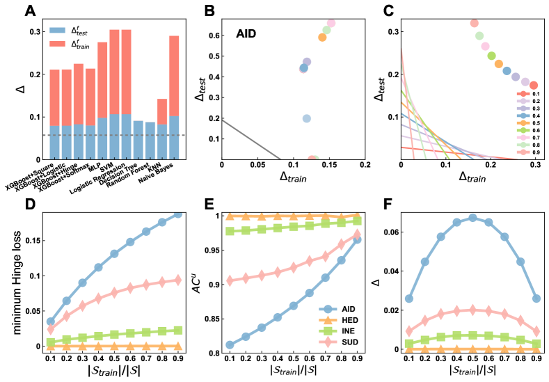
Fig. 2: Detailed evaluation of expected errors ($\Delta$) across all feature vectors for each dataset. Panels A and B showcase the error dynamics for the AID dataset during training ($\Delta_{train}^{f}$) and testing ($\Delta_{test}^{f}$) phases, considering a random division ratio where the training set size $|\mathcal{S}_{train}|$ constitutes 70% of the total set size $|\mathcal{S}|$. (A) The dashed line indicates the expected error of the optimal classifier as determined by Eq. 5. (B) Illustrates the correlation between $\Delta_{train}^{f}$ and $\Delta_{test}^{f}$, contrasting the theoretical solution outlined in Eq. 5 (gray line) against empirical observations from diverse binary classifiers (represented by dots). (C) Explores the interplay between $\Delta_{train}^{f}$ and $\Delta_{test}^{f}$ under a spectrum of random division ratios $|\mathcal{S}_{train}|/|\mathcal{S}|$, varying from 10% to 90%. (D-F) depict the expected errors or performance metrics for each dataset under different random divisions: (D) Hinge loss, (E) upper bound of accuracy ($AC^{u}$), and (F) anticipated optimal errors ($\Delta$). In these panels, dots correspond to numerical results derived from the data divisions, while lines represent the theoretical predictions adjusted for the respective division ratios (as detailed in Eqs. 54 and 56 within the SI Appendix, Random Division).

In Fig. 2, we investigate at length the characteristics of both training and test sets in order to comprehensively understand the generalization ability of the proposed boundary theory. It shows that, the theoretical optimal loss for $\Delta$ is smaller than that of any representative classier, suggesting that the predictability of available classifiers are still a certain distance from the theoretical upper limit, both for a specific division (i.e. $|\mathcal{S}_{train}|/|\mathcal{S}|=70\%$, Fig. 2A) or all possible random divisions (Fig. 2C). Therefore, $\Delta_{train}^{f}$ and $\Delta_{test}^{f}$ are respectively equivalent to the learning and generalization differences in supervised machine learning. If one aims at obtaining the upper bound of a given dataset (corresponds to $\Delta$), he or she needs to minimize simultaneously both $\Delta_{train}^{f}$ and $\Delta_{test}^{f}$ Jiang et al. (2019). However, on one hand, it requires fitting training data as much as possible to obtain minimal $\Delta_{train}^{f}$, often leading to the overfitting problem Ying (2019); Bartlett et al. (2020), which further dilutes the generalization ability (corresponds to greater $\Delta_{test}^{f}$ and more distant from the upper bound). On the other hand, one may try to solve such dilemma by early-stopping, dropout or adding regularization items Srivastava et al. (2014); Ying (2019), resulting in a greater learning loss (corresponds to larger $\Delta_{train}^{f}$), leaving an unstable prediction.

Fig. 2D shows a general increase of learning loss with the size of training set ($|\mathcal{S}_{train}|$), which converges to a certain limit if the feeding schema is sufficient enough. Comparatively, the upper bound ($\text{AC}^{u}$) monotonically increases with $|\mathcal{S}_{train}|$ (Fig. 2E), which agrees with the common sense that more knowledge can be extracted by adding more sources. The good agreements are additional proved theoretically by giving an arbitrary parameter governing the ratio of random divisions (represented by solid lines in Fig. 2D-2F, see also SI Appendix, Random Division). Furthermore, Fig. 2F shows that the optimal error ($\Delta$) will be achieved when the training set is either adequate large or small enough as its expectation is symmetric based on SI Appendix, Eq. 56.

Effect of Overlapping Ratio of Samples.
The relationship between the distribution pattern of feature vectors, specifically the overlapping ratio of data samples, and the expected upper bounds ($\text{AR}^{u}$) is investigated. To ascertain the minimum and maximum values of $\text{AR}^{u}$, we formulate two optimization problems as follows:

$$\text{AR}^{u}_{\min}(D_{\mathcal{S}})=\min\Big{\{}\text{AR}^{u}(\mathcal{P},\mathcal{N})\mid D_{\mathcal{S}}(\mathcal{P},\mathcal{N})=D_{\mathcal{S}}\Big{\}}$$ (7)

and

$$\text{AR}^{u}_{\max}(D_{\mathcal{S}})=\max\Big{\{}\text{AR}^{u}(\mathcal{P},\mathcal{N})\mid D_{\mathcal{S}}(\mathcal{P},\mathcal{N})=D_{\mathcal{S}}\Big{\}}.$$ (8)

In these equations, $D_{\mathcal{S}}(\mathcal{P},\mathcal{N})=1-J(\mathcal{P}||\mathcal{N})$ denotes the overlapping ratio between positive and negative samples, with $J(\mathcal{P}||\mathcal{N})$ being the Jensen-Shannon divergence Menéndez et al. (1997) between the normalized distributions $\mathcal{P}$ and $\mathcal{N}$. At the extremes, $D_{\mathcal{S}}=1$ signifies complete overlap, whereas $D_{\mathcal{S}}=0$ indicates complete separation.

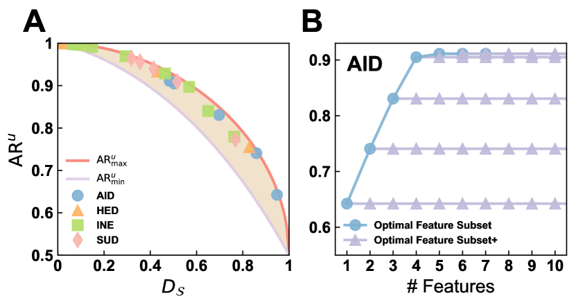
Fig. 3: Characterization of the upper bound for AUC-ROC ($\text{AR}^{u}$) as influenced by key dataset properties on the AID dataset, with extended results for additional datasets available in the SI Appendix, Fig. S6. (A) Illustrates how $\text{AR}^{u}$ varies with the degree of overlap ($D_{\mathcal{S}}$) between positive and negative sample distributions. The red and purple curves denote the theoretically expected maximum and minimum bounds, respectively. The plotted dots represent the empirically obtained optimal AUC scores corresponding to different overlapping scenarios facilitated by feature selection. (B) Depicts the relationship between $\text{AR}^{u}$ and the number of features, where the blue curve indicates the maximum upper bounds achievable with a specified number of features within the optimal feature subset. The purple curves denote the maximal upper bounds achievable when the optimal feature subset is expanded by the inclusion of additional arbitrary feature transformations, referred to as the optimal feature subset+.

By employing numerical simulations and heuristic methods (see SI Appendix, Overlapping and Boundary for details), we deduce the optimal solutions for these optimization problems as $\text{AR}^{u}_{\min}$ and $\text{AR}^{u}_{\max}$. Fig. 3A illustrates a monotonic decrease in both $\text{AR}^{u}_{\min}$ and $\text{AR}^{u}_{\max}$ as $D_{\mathcal{S}}$ increases, with the upper bounds for all four datasets analyzed resting between these values. This suggests that greater overlap between positive and negative samples correlates with a reduction in the achievable upper bound for binary classification performance. In the limit, the upper bound can attain $1$ (perfect accuracy) when $D_{\mathcal{S}}=0$, and $0.5$ (equivalent to random guessing) when $D_{\mathcal{S}}=1$.

Effect of Feature Selection.
The influence of feature selection on the upper bound is scrutinized. Fig. 3B presents a case study utilizing the AID dataset. It is observed that the upper bound tends to rise with the inclusion of additional features. Nevertheless, there exists a specific subset of features—the optimal feature subset—that is adequate to reach the potential upper bound for the majority of datasets. Beyond this subset, incorporating more features does not enhance the upper bound. It is also noted that integrating transformations of features from the optimal subset fails to provide any further increase in the upper bound. Collectively, these insights underscore the efficacy of our methodology in streamlining the binary classification process by pinpointing the most effective subset of features for feature engineering purposes.

Conclusion and Discussion
This research delves into the impact that characteristics of features have on the upper limit of predictive accuracy in binary classification endeavors. Through a combination of theoretical analysis and numerical experimentation, we have shed light on the pivotal roles played by data distribution and feature selection in determining the ceiling of a model’s performance. Additionally, we introduce a quantitative assessment of error balance ($\Delta$), which offers insights into the practicality of reaching these upper bounds in both training and testing scenarios.

The implications of our findings for machine learning (ML) are substantial. We have empirically confirmed that datasets with greater overlap among samples pose more significant challenges for accurate classification. Our theoretical framework convincingly demonstrates that expanding the feature set can reduce overlap between classes and push the boundaries of predictive performance higher. Therefore, in the context of raw data, the discovery and curation of new features, along with the strategic selection of an optimal subset, are crucial for maximizing the efficacy of model training. On the other hand, relying solely on transformations of existing features does not contribute to an improvement of the upper performance limit.

Nonetheless, our study has limitations. Firstly, the theoretical upper bound of prediction performance is attainable only in an ideal scenario where all distinct samples are correctly classified, which does not account for the balance between data availability and model complexity. In real-world applications, achieving this upper bound is often challenging due to constraints on data and computational resources. The degree to which the upper bound can be approached is contingent upon the data distribution, and a theoretical framework to quantify this degree is an avenue for future investigation. Secondly, our analysis presumes that the data space is discretized. The practical utility of the derived upper bound would benefit from considering the distance and similarity between data samples, which we have not addressed. We advocate for future studies that explore the implications of limited model complexity and the behavior in a continuous data space.

Expanding beyond the realm of binary classification, the principles of our boundary theory could also enhance our comprehension of multiclass classification issues, which can be segmented into a series of binary classification challenges. Looking ahead, our forthcoming endeavors will concentrate on the predictability and interpretability within a more applied framework, particularly concerning feature engineering, given classifiers, optimization techniques, and energy landscapes. In subsequent research, we aim to advance the predictability of ML and AI systems, enhancing the trustworthiness of AI by improving our ability to explain, manage, and regulate these systems.

Methods & Materials
Objective Functions.
Square Loss. It is denoted based on the square error between the predicted class and actual label for every instance dataset Körding and Wolpert (2004), reads

$$\min_{g}\ \frac{1}{m}\sum\limits_{x_{i}}\Big{(}g(x_{i})-y_{i}\Big{)}^{2}.$$

Its corresponding optimal classifier must satisfy,

$$g^{*}_{\text{Square}}(x_{i})=p_{+}(x_{i})-p_{-}(x_{i}),$$ (9)

for every $x_{i}\in\mathcal{S}$.

Logistic Loss. The Logistic loss is defined as Ahmed and Xing (2009),

$$\min_{g}\ \frac{1}{m}\sum\limits_{x_{i}}-y_{i}\log g(x_{i})-\Big{(}1-y_{i}\Big{)}\log\Big{(}1-g(x_{i})\Big{)}$$

Its corresponding optimal classifier must satisfy,

$$g^{*}_{\text{Logistic}}(x_{i})=p_{+}(x_{i})-p_{-}(x_{i}),$$ (10)

for every $x_{i}\in\mathcal{S}$.

Hinge Loss. Hinge loss aims to maximize the margin between the decision boundary and data points Xu et al. (2017), reads

$$\min_{g}\ \frac{1}{2m}\sum\limits_{x_{i}}\max\Big{\{}0,1-g(x_{i})y_{i}\Big{\}}.$$

Its corresponding optimal classifier must satisfy,

$$g^{*}_{\text{Hinge}}(x_{i})=\left\{\begin{aligned} 1&&\mathcal{P}(x_{i})\geq\mathcal{N}(x_{i})\\ -1&&\mathcal{P}(x_{i})<\mathcal{N}(x_{i}),\end{aligned}\right.$$ (11)

for every $x_{i}\in\mathcal{S}$.

Softmax Loss. Assume that $f(x_{i})$ is the probability that data with feature vector $x_{i}$ belongs to positive class Wang et al. (2018), reads

$$\min_{g}\ \frac{1}{m}\sum\limits_{x_{i}}-\log g(x_{i})-\log\Big{(}1-g(x_{i})\Big{)}.$$

Its corresponding optimal classifier must satisfy,

$$g^{*}_{\text{Softmax}}(x_{i})=p_{+}(x_{i}),$$ (12)

for every $x_{i}\in\mathcal{S}$.

The mathematical details for these optimal classifiers (Eqs. 9-12) of corresponding objective functions can be found in SI Appendix, Objective Functions.

Acknowledge
This work was supported by the National Natural Science Foundation of China (Grant Nos. 72371224 and 71972164), the Major Project of The National Social Science Fund of China (Grant No. 19ZDA324), the Research Grants Council of the Hong Kong Special Administrative Region (Grant No. 11218221) and the Fundamental Research Funds for the Central Universities.

Table 1: Comprehensive experimental results and theoretical upper bound analysis for various binary classifiers on four real datasets. The classifiers evaluated include XGBoost, Multilayer Perceptron (MLP), Support Vector Machine (SVM), Logistic Regression (LR), Decision Tree (DT), Random Forest (RF), K-Nearest Neighbors (KNN), and Naive Bayes (NB). Performance metrics for each classifier are presented in terms of area under the ROC curve (AUC-ROC, abbreviated as AR), area under the Precision-Recall curve (AUC-PR, abbreviated as AP), and Accuracy (AC).

Data	Metrics	XGBoost				MLP	SVM	LR	DT	RF	KNN	NB	Boundaries
		Square	Logistic	Hinge	Softmax
AID	AR	0.6941	0.6917	0.6096	0.6223	0.5777	0.5	0.4921	0.7863	0.7961	0.7464	0.5228	0.9112
	AP	0.6517	0.6491	0.5245	0.5373	0.4939	0.4454	0.4424	0.7232	0.7065	0.6483	0.4606	0.8806
	AC	0.6491	0.6476	0.634	0.6469	0.5957	0.5546	0.5546	0.8015	0.8015	0.7533	0.5692	0.8015
HED	AR	0.7959	0.7948	0.7249	0.7337	0.6127	0.595	0.619	0.9998	0.9997	0.7149	0.6103	1.0
	AP	0.7702	0.769	0.6541	0.6652	0.5767	0.5562	0.574	0.9998	0.9996	0.6523	0.5667	1.0
	AC	0.7349	0.7347	0.7249	0.7337	0.6126	0.595	0.619	0.9998	0.9997	0.7149	0.6103	0.9998
INE	AR	0.9275	0.9239	0.7543	0.7788	0.7467	0.6229	0.6737	0.9728	0.9638	0.794	0.7336	0.9983
	AP	0.9751	0.9738	0.8659	0.8778	0.8627	0.8071	0.829	0.9844	0.9783	0.886	0.8577	0.9993
	AC	0.8734	0.8699	0.857	0.8704	0.839	0.8008	0.8043	0.9764	0.9764	0.8635	0.7913	0.9764
SUD	AR	0.9645	0.9322	0.8807	0.8603	0.6855	0.7206	0.665	0.8742	0.8807	0.8105	0.6773	0.9649
	AP	0.9396	0.9031	0.7973	0.7848	0.5309	0.5822	0.514	0.8028	0.7973	0.6845	0.5038	0.9381
	AC	0.9038	0.8942	0.9038	0.8942	0.7596	0.7885	0.75	0.9038	0.9038	0.8462	0.7404	0.9038

References

- Hastie et al. (2009) T. Hastie, R. Tibshirani, J. H. Friedman, and J. H. Friedman, The elements of statistical learning: data mining, inference, and prediction, vol. 2 (Springer, 2009).
- Agresti (2012) A. Agresti, Categorical data analysis, vol. 792 (John Wiley & Sons, 2012).
- Noble (2006) W. S. Noble, Nature Biotechnology 24, 1565 (2006).
- Chen and Guestrin (2016) T. Chen and C. Guestrin, in Proceedings of the 22nd acm sigkdd international conference on knowledge discovery and data mining (2016), pp. 785–794.
- Rosasco et al. (2004) L. Rosasco, E. De Vito, A. Caponnetto, M. Piana, and A. Verri, Neural Computation 16, 1063 (2004).
- Cortes and Mohri (2003) C. Cortes and M. Mohri, Advances in neural information processing systems 16 (2003).
- Yang and Ying (2022) T. Yang and Y. Ying, ACM Computing Surveys 55, 1 (2022).
- Joachims (2005) T. Joachims, in Proceedings of the 22nd international conference on Machine learning (2005), pp. 377–384.
- Ying et al. (2016) Y. Ying, L. Wen, and S. Lyu, Advances in neural information processing systems 29 (2016).
- Norton and Uryasev (2019) M. Norton and S. Uryasev, Mathematical Programming 174, 575 (2019).
- Yuan et al. (2021) Z. Yuan, Y. Yan, M. Sonka, and T. Yang, in Proceedings of the IEEE/CVF International Conference on Computer Vision (2021), pp. 3040–3049.
- Gao and Zhou (2012) W. Gao and Z.-H. Zhou, in International Joint Conference on Artificial Intelligence (2012), URL https://api.semanticscholar.org/CorpusID:11266780.
- Lei et al. (2020) Y. Lei, A. Ledent, and M. Kloft, Advances in Neural Information Processing Systems 33, 21236 (2020).
- Fawcett (2006) T. Fawcett, Pattern Recognition Letters 27, 861 (2006).
- Sun et al. (2020) J. Sun, L. Feng, J. Xie, X. Ma, D. Wang, and Y. Hu, Nature communications 11, 574 (2020).
- Lü et al. (2015) L. Lü, L. Pan, T. Zhou, Y.-C. Zhang, and H. E. Stanley, Proceedings of the National Academy of Sciences 112, 2325 (2015).
- Majnik and Bosnić (2013) M. Majnik and Z. Bosnić, Intelligent data analysis 17, 531 (2013).
- Metz (1978) C. E. Metz, in Seminars in nuclear medicine (Elsevier, 1978), vol. 8, pp. 283–298.
- Fawcett (2001) T. Fawcett, in Proceedings 2001 IEEE International Conference on Data Mining (2001), pp. 131–138.
- Bohr et al. (1928) N. Bohr et al., The quantum postulate and the recent development of atomic theory, vol. 3 (Printed in Great Britain by R. & R. Clarke, Limited, 1928).
- Menard (2002) S. Menard, Applied logistic regression analysis, 106 (Sage, 2002).
- Hosmer Jr et al. (2013) D. W. Hosmer Jr, S. Lemeshow, and R. X. Sturdivant, Applied logistic regression, vol. 398 (John Wiley & Sons, 2013).
- Haykin (1998) S. Haykin, Neural networks: a comprehensive foundation (Prentice Hall PTR, 1998).
- Albawi et al. (2017) S. Albawi, T. A. Mohammed, and S. Al-Zawi, in 2017 International Conference on Engineering and Technology (ICET) (2017), pp. 1–6.
- Brown et al. (2000) M. P. Brown, W. N. Grundy, D. Lin, N. Cristianini, C. W. Sugnet, T. S. Furey, M. Ares Jr, and D. Haussler, Proceedings of the National Academy of Sciences 97, 262 (2000).
- Kingsford and Salzberg (2008) C. Kingsford and S. L. Salzberg, Nature Biotechnology 26, 1011 (2008).
- Safavian and Landgrebe (1991) S. Safavian and D. Landgrebe, IEEE Transactions on Systems, Man, and Cybernetics 21, 660 (1991).
- Hanley and McNeil (1982) J. A. Hanley and B. J. McNeil, Radiology 143, 29 (1982).
- Bradley (1997) A. P. Bradley, Pattern Recognition 30, 1145 (1997).
- Tran et al. (2017) N. H. Tran, X. Zhang, L. Xin, B. Shan, and M. Li, Proceedings of the National Academy of Sciences 114, 8247 (2017).
- Congalton (1991) R. G. Congalton, Remote Sensing of Environment 37, 35 (1991).
- Madani et al. (2018) A. Madani, R. Arnaout, M. Mofrad, and R. Arnaout, NPJ Digital Medicine 1, 6 (2018).
- Kim et al. (2021) S.-C. Kim, A. S. Arun, M. E. Ahsen, R. Vogel, and G. Stolovitzky, Proceedings of the National Academy of Sciences 118, e2100761118 (2021).
- Liu et al. (2023) Y. Liu, H. Zhao, J. Gu, Y. Qiao, and C. Dong, IEEE Transactions on Pattern Analysis and Machine Intelligence pp. 1–16 (2023).
- Xu et al. (2015) J. Xu, Y. Y. Tang, B. Zou, Z. Xu, L. Li, Y. Lu, and B. Zhang, IEEE Transactions on Cybernetics 45, 1169 (2015).
- Bartlett et al. (2020) P. L. Bartlett, P. M. Long, G. Lugosi, and A. Tsigler, Proceedings of the National Academy of Sciences 117, 30063 (2020).
- Jiang et al. (2019) Y. Jiang, D. Krishnan, H. Mobahi, and S. Bengio, in International Conference on Learning Representations (2019), URL https://openreview.net/forum?id=HJlQfnCqKX.
- Ying (2019) X. Ying, in Journal of Physics: Conference Series (IOP Publishing, 2019), vol. 1168, p. 022022.
- Srivastava et al. (2014) N. Srivastava, G. Hinton, A. Krizhevsky, I. Sutskever, and R. Salakhutdinov, The journal of machine learning research 15, 1929 (2014).
- Menéndez et al. (1997) M. Menéndez, J. Pardo, L. Pardo, and M. Pardo, Journal of the Franklin Institute 334, 307 (1997).
- Körding and Wolpert (2004) K. P. Körding and D. M. Wolpert, Proceedings of the National Academy of Sciences 101, 9839 (2004).
- Ahmed and Xing (2009) A. Ahmed and E. P. Xing, Proceedings of the National Academy of Sciences 106, 11878 (2009).
- Xu et al. (2017) G. Xu, Z. Cao, B.-G. Hu, and J. C. Principe, Pattern Recognition 63, 139 (2017).
- Wang et al. (2018) F. Wang, J. Cheng, W. Liu, and H. Liu, IEEE Signal Processing Letters 25, 926 (2018).