tablesection algorithmsection
Bayesian Optimization with Noise-Free Observations:
Improved Regret Bounds via Random Exploration
Abstract
This paper studies Bayesian optimization with noise-free observations. We introduce new algorithms rooted in scattered data approximation that rely on a random exploration step to ensure that the fill-distance of query points decays at a near-optimal rate. Our algorithms retain the ease of implementation of the classical GP-UCB algorithm and satisfy cumulative regret bounds that nearly match those conjectured in [31], hence solving a COLT open problem. Furthermore, the new algorithms outperform GP-UCB and other popular Bayesian optimization strategies in several examples.
1 Introduction
Bayesian optimization [12, 17, 9] is an attractive strategy for global optimization of black-box objective functions. Bayesian optimization algorithms sequentially acquire information on the objective by observing its value at carefully selected query points. In some applications, these observations are noisy, but in many others the objective can be noiselessly observed; examples include hyperparameter tuning for machine learning algorithms [3], parameter estimation for computer models [7, 21], goal-driven dynamics learning [1], and alignment of density maps in Wasserstein distance [28]. While most Bayesian optimization algorithms can be implemented with either noisy or noise-free observations, few methods and theoretical analyses are tailored to the noise-free setting.
This paper introduces two new algorithms rooted in scattered data approximation for Bayesian optimization with noise-free observations. The first algorithm, which we call GP-UCB+, supplements query points obtained via the classical GP-UCB algorithm [24] with randomly sampled query points. The second algorithm, which we call EXPLOIT+, supplements query points obtained by maximizing the posterior mean of a Gaussian process surrogate model with randomly sampled query points. Both algorithms retain the simplicity and ease of implementation of the GP-UCB algorithm, but introduce an additional random exploration step to ensure that the fill-distance of query points decays at a near-optimal rate. The new random exploration step has a profound impact on both theoretical guarantees and empirical performance. On the one hand, GP-UCB+ and EXPLOIT+ satisfy regret bounds that improve upon existing and refined rates for the GP-UCB algorithm. Indeed, the new algorithms nearly achieve the cumulative regret bounds for noise-free bandits conjectured in [31]. On the other hand, GP-UCB+ and EXPLOIT+ explore the state space faster, which leads to an improvement in numerical performance across a range of benchmark and real-world examples.
1.1 Main Contributions
-
•
We introduce two new algorithms, GP-UCB+ and EXPLOIT+, which attain the cumulative regret bounds for noise-free bandits conjectured in [31], and far improve existing and refined rates for the classical GP-UCB algorithm. Our theory covers both deterministic assumptions on the objective (Theorem 4.4) and probabilistic ones (Theorem 4.8). En route to compare the cumulative regret bounds for our new algorithms with those for GP-UCB, we establish in Theorem 3.1 a regret bound for GP-UCB with squared exponential kernels that refines the one in [16].
-
•
Our algorithms and regret bounds bring ideas from the literature on scattered data approximation [33] to the design and analysis of Bayesian optimization algorithms. Such ideas are particularly powerful in the noise-free setting, where the maximum information gain used in the analysis of the noisy setting is not well defined [24].
-
•
We numerically demonstrate that GP-UCB+ and EXPLOIT+ outperform GP-UCB and other popular Bayesian optimization algorithms across many examples, including optimization of several -dimensional benchmark objective functions, hyperparameter tuning for random forests, and optimal parameter estimation of a garden sprinkler computer model.
-
•
We showcase that both GP-UCB+ and EXPLOIT+ share the simplicity and ease of implementation of the GP-UCB algorithm. In addition, EXPLOIT+ requires fewer input parameters than GP-UCB or GP-UCB+, and achieves competitive empirical performance without any tuning.
1.2 Outline
Section 2 formalizes the problem of interest and provides necessary background. We review related work in Section 3. Our new algorithms are introduced in Section 4, where we establish regret bounds under deterministic and probabilistic assumptions on the objective. Section 5 contains numerical examples, and we close in Section 6. Proofs and additional numerical experiments are deferred to an appendix.
2 Preliminaries
2.1 Problem Statement
We want to find the global maximizer of an objective function by leveraging the observed values of at carefully chosen query points. We are interested in the setting where the observations of the objective are noise-free, i.e. for query points we can access observations The functional form of is not assumed to be known. For simplicity, we assume throughout that is a -dimensional hypercube.
Our theory will cover both deterministic and probabilistic assumptions on the objective In the deterministic case, we assume that belongs to the Reproducing Kernel Hilbert Space (RKHS) associated with a kernel . In the probabilistic case, we assume that is a draw from a centered Gaussian process with covariance function .
2.2 Gaussian Processes and Bayesian Optimization
Many Bayesian optimization algorithms, including the ones introduced in this paper, rely on a Gaussian process surrogate model of the objective function to guide the choice of query points. Here, we review the main ideas. Denote generic query locations by and the corresponding noise-free observations by Gaussian process interpolation with a prior yields the following posterior predictive mean and variance:
where and is a matrix with entries .
Our interest lies in Bayesian optimization with noise-free observations. However, we recall for later reference that if the observations are noisy and take the form where then the posterior predictive mean and variance are given by
where
To perform Bayesian optimization, one can sequentially select query points by optimizing a Gaussian Process Upper Confidence Bound (GP-UCB) acquisition function. Let denote the query points at the -th iteration of the algorithm. Then, at the -th iteration, the classical GP-UCB algorithm [24] sets
| (2.1) |
where is a user-chosen positive parameter. The posterior predictive mean provides a surrogate model for the objective; hence, one expects the maximum of to be achieved at a point where is large. However, the surrogate model may not be accurate at points where is large, and selecting query points with large predictive variance helps improve the accuracy of the surrogate model. The GP-UCB algorithm finds a compromise between exploitation (maximizing the mean) and exploration (maximizing the variance). The weight parameter balances this exploitation-exploration trade-off. For later discussion, Algorithm 1 below summarizes the approach with noise-free observations and
-
1.
Set
-
2.
Set and .
-
3.
Update and using and
2.3 Performance Metric
The performance of Bayesian optimization algorithms is often analyzed through bounds on their cumulative regret, given by
where is the maximum of the objective is the query location selected at the -th iteration, and is called the instantaneous regret. Algorithms that satisfy are known as zero-regret algorithms. In the large asymptotic, zero-regret algorithms successfully recover the maximum of the objective since
2.4 Choice of Kernel
We will consider the well-specified setting where Gaussian process interpolation for surrogate modeling is implemented using the same kernel which specifies the deterministic or probabilistic assumptions on namely or The impact of kernel misspecification on Bayesian optimization algorithms is studied in [2, 15].
For concreteness, we focus on Matérn kernels with smoothness parameter and lengthscale parameter , given by
where is a modified Bessel function of the second kind, and on squared exponential kernels with lengthscale parameter , given by
We recall that the Matérn kernel converges to the squared exponential kernel in the large asymptotic. Both types of kernel are widely used in practice, and we refer to [34, 33, 26] for further background.
3 Related Work
3.1 Existing Regret Bounds: Noisy Observations
Numerous works have established cumulative regret bounds for Bayesian optimization with noisy observations under both deterministic and probabilistic assumptions on the objective function [24, 5, 32, 2, 22, 14]. These bounds involve a quantity known as the maximum information gain, which under a Gaussian noise assumption is given by where represents the noise level. In particular, under a deterministic objective function assumption, [5] showed a cumulative regret bound for GP-UCB of the form , which improves the one obtained in [24] by a factor of . By tightening existing upper bounds on the maximum information gain, [32] established a cumulative regret bound for GP-UCB of the form
for Matérn and squared exponential kernels.
3.2 Existing Regret Bounds: Noise-Free Observations
In contrast to the noisy setting, few works have obtained regret bounds with noise-free observations. With an expected improvement acquisition function and Matérn kernel, [4] provides a simple regret bound of the form , where suppresses logarithmic factors. [8] introduced a branch and bound algorithm that achieves an exponential rate of convergence for the instantaneous regret. However, unlike the standard GP-UCB algorithm, the algorithm in [8] requires many observations in each iteration to reduce the search space, and it further requires solving a constrained optimization problem in the reduced search space.
To the best of our knowledge, [16] presents the only cumulative regret bound available for GP-UCB with noise-free observations under a deterministic assumption on the objective. Specifically, they consider Algorithm 1, and, noticing that for any , they deduce that existing cumulative regret bounds for Bayesian optimization with noisy observations remain valid with noise-free observations. Furthermore, in the noise-free setting, the cumulative regret bound is improved by a factor of , which comes from using a constant weight parameter given by the squared RKHS norm of the objective. This leads to a cumulative regret bound with rate , which gives
| (3.1) |
for Matérn and squared exponential kernels. A similar improvement has not been established under a probabilistic assumption on the objective.
3.3 Tighter Bound for Squared Exponential Kernels
[31] sets as an open problem whether one can improve the cumulative regret bounds in (3.1) for the GP-UCB algorithm with noise-free observations. For squared exponential kernels, we claim that one can further improve the cumulative regret bound in (3.1) by a factor of .
Theorem 3.1.
Let , where is a squared exponential kernel. GP-UCB with noise-free observations and satisfies the cumulative regret bound
Remark 3.2.
Our improvement in the bound comes from a constant term , which was ignored in existing analyses with noisy observations. By letting , the constant offsets a growth in the cumulative regret bound.
Remark 3.3.
For Matérn kernels, a similar approach to improve the rate is not feasible. A state-of-the-art, near-optimal upper bound on the maximum information gain with Matérn kernels obtained in [32] introduces a polynomial growth factor as the noise variance decreases to zero. Minimizing the rate of an upper bound in [32] one can match the rate obtained in [16].
3.4 Conjectured Regret Bounds
Theorem 3.1 refines the rate bound in (3.1) for GP-UCB with noise-free observations using squared exponential kernels. In the rest of the paper, we will design new algorithms that achieve drastically faster rates. In particular, we are motivated by [31], which conjectured that, for Matérn kernels, a cumulative regret bound
could be obtained. Our new algorithms nearly achieve this bound while preserving the ease of implementation of GP-UCB algorithms. The recent preprint [27] proposes an alternative batch-based approach, which combines random sampling with domain shrinking to attain the conjectured rates with high probability.
4 Exploitation with Accelerated Exploration
4.1 How Well Does GP-UCB Explore?
The GP-UCB algorithm selects query points by optimizing an acquisition function which incorporates the posterior mean to promote exploitation and the posterior standard deviation to promote exploration. Our new algorithms are inspired by the desire to improve the exploration of GP-UCB. Before introducing the algorithms in the next subsection, we heuristically explain why such an improvement may be possible.
A natural way to quantify how well data cover the search space is via the fill-distance, given by
The fill-distance appears in error bounds for Gaussian process interpolation and regression [33, 29, 25, 30]. For quasi-uniform points, it holds that , which is the fastest possible decay rate for any sequence of design points. The fill-distance of the query points selected by our new Bayesian optimization algorithms will (nearly) decay at this rate.
[36] introduced a stabilized greedy algorithm to obtain query points by maximizing the posterior predictive standard deviation at each iteration. Their algorithm sequentially generates a set of query points whose fill-distance decays at a rate by sequentially solving constrained optimization problems, which can be computationally demanding. Since GP-UCB simply promotes exploration through the posterior predictive standard deviation term in the UCB acquisition function, one may heuristically expect the fill-distance of query points selected by the standard GP-UCB algorithm to decay at a slower rate. On the other hand, a straightforward online approach to obtain a set of query points whose fill-distance nearly decays at a rate is to sample randomly from a probability measure with a strictly positive Lebesgue density on Specifically, [18] shows that, in expectation, the fill-distance of independent samples from such a measure decays at a near-optimal rate: for any
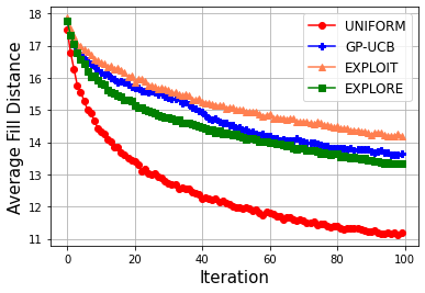
Figure 1 compares the decay of the fill-distance for query points selected using four strategies. For a 10-dimensional Rastrigin function, we consider: (i) GP-UCB; (ii) EXPLOIT (i.e., maximizing the posterior mean at each iteration); (iii) EXPLORE (i.e., maximizing the posterior variance); and (iv) UNIFORM (i.e. independent uniform random samples on ). The results were averaged over 100 independent experiments. The fill-distance for GP-UCB lies in between those for EXPLORE and EXPLOIT; whether it lies closer to one or the other depends on the choice of weight parameter, which here we choose based on a numerical approximation of the max-norm of the objective, where is a discretization of the search space . Note that UNIFORM yields a drastically smaller fill-distance even when compared with EXPLORE. Our new algorithms will leverage random sampling to enhance exploration in Bayesian optimization and achieve improved regret bounds.
4.2 Improved Exploration via Random Sampling
In this subsection, we introduce two Bayesian optimization algorithms that leverage random sampling as a tool to facilitate efficient exploration of the search space. While the GP-UCB algorithm selects a single query point per iteration, our algorithms select two query points per iteration.
The first algorithm we introduce, which we call GP-UCB+, selects a query point using the GP-UCB acquisition function and another query point by random sampling. We outline the pseudocode in Algorithm 2. The second algorithm we introduce, which we call EXPLOIT+, decouples the exploitation and exploration goals, selecting one query point by maximizing the posterior mean to promote exploitation, and another query point by random sampling to promote exploration. We outline the pseudocode in Algorithm 3.
-
1.
Exploitation + Exploration: Set
-
2.
Exploration: Sample
-
3.
Set
-
4.
Update and using and
-
1.
Exploitation: Set
-
2.
Exploration: Sample
-
3.
Set
-
4.
Update using and
Notably, EXPLOIT+ does not require input weight parameters As mentioned in Section 3, many regret bounds for GP-UCB algorithms rely on choosing the weight parameters as the squared RKHS norm of the objective or in terms of a bound on it. The performance of GP-UCB and GP-UCB+ can be sensitive to this choice, which in practice is often based on empirical tuning or heuristic arguments rather than guided by the theory. In contrast, EXPLOIT+ achieves the same regret bounds as GP-UCB+ and drastically faster rates than GP-UCB without requiring the practitioner to specify weight parameters. Additionally, EXPLORE+ shows competitive empirical performance.
Remark 4.1.
Remark 4.2.
A common heuristic strategy to expedite the performance of Bayesian optimization algorithms is to acquire a moderate number of initial design points by uniformly sampling the search space. Since the order of the exploration and exploitation steps can be swapped in our algorithms, such heuristic strategy can be interpreted as an initial batch exploration step.
Remark 4.3.
A natural choice for is the uniform distribution on the search space . Our theory, which utilizes bounds on the fill-distance of randomly sampled query points from [18], holds as long as has a strictly positive Lebesgue density on In what follows, we assume throughout that satisfies this condition.
4.3 Regret Bounds: Deterministic Setting
We first obtain regret bounds under the deterministic assumption that belongs to the RKHS of a kernel Our algorithms are random due to sampling from and we show cumulative regret bounds in expectation with respect to such randomness.
Theorem 4.4.
Let GP-UCB+ with and EXPLOIT+ attain the following cumulative regret bounds. For Matérn kernels with parameter ,
where can be arbitrarily small. For squared exponential kernels,
Remark 4.5.
Remark 4.6.
Compared with the GP-UCB algorithm with noise-free observations, the proposed algorithms attain improved cumulative regret bounds in expectation for both Matérn and squared exponential kernels. For the Matérn kernel, the new cumulative regret bound satisfies a slower polynomial growth rate and completely removes the log factor. For the squared exponential kernel, the proposed algorithms have bounded cumulative regret, whereas the improved bound for the GP-UCB algorithm in Theorem 3.1 grows at rate .
Remark 4.7.
For Matérn kernels, compared with the recent preprint [27], which attains rate when , our algorithms achieve bounded cumulative regret. When , [27] attains the rate conjectured in [31] up to a logarithmic factor, while we attain the conjectured rate up to a factor of , for arbitrarily small . Our result additionally covers squared exponential kernels, for which we show bounded cumulative regret.
4.4 Regret Bounds: Probabilistic Setting
Next, we provide regret bounds under the probabilistic assumption that is a draw from a Gaussian process with covariance To this end, let and assume the following high probability bound on the derivatives of GP sample paths : for some constants ,
For squared exponential and Matérn kernels with smoothness parameter , the above condition is met, while it is violated for the Ornstein-Uhlenbeck kernel [10, 26].
Theorem 4.8.
Suppose . For any GP-UCB+ with and EXPLOIT+ satisfy the following cumulative regret bounds with probability at least For Matérn kernels with parameter
where can be arbitrarily small. For squared exponential kernels,
Remark 4.9.
Recall that under the RKHS assumption, [16] shows an factor improvement in the noise-free observation setting compared with the noisy case thanks to the constant exploration parameter in the GP-UCB algorithm. However, under the Gaussian process assumption, we need to increase the exploration parameter. Therefore, no additional improvement can be made under the noise-free setting over the noisy case.
Remark 4.10.
Compared with GP-UCB with noisy observations, where [32] shows regret bounds and for Matérn and squared exponential kernels, the proposed algorithms achieve significantly faster rates in expectation.
5 Numerical Experiments
This section explores the empirical performance of our methods on three benchmark objective functions, on hyperparameter tuning for a machine learning model, and on optimizing a black-box objective function designed to guide engineering decisions. We compare the new algorithms (GP-UCB+, EXPLOIT+) with GP-UCB and two other popular Bayesian optimization strategies: Expected Improvement (EI) and Probability of Improvement (PI). We also compare with the EXPLOIT approach outlined in Subsection 4.1, but not with EXPLORE as this method did not achieve competitive performance. Throughout, we choose the distribution which governs random exploration in the new algorithms to be uniform on . For the weight parameter of UCB acquisition functions, we considered a well-tuned constant value that achieves good performance in our examples, and the approach in [6], which sets where is a discretization of the search space. All the hyperparameters of the kernel function were iteratively updated through maximum likelihood estimation. Since the new algorithms need two noise-free observations per iteration but the methods we compare with only need one, we run the new algorithms for half as many iterations to ensure a fair comparison.
5.1 Benchmark Objective Functions
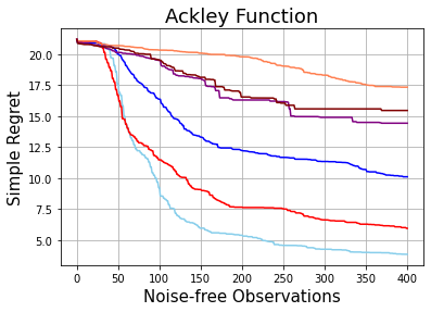
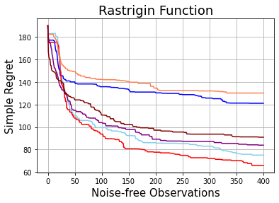
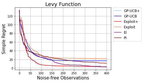
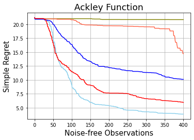
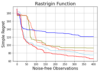
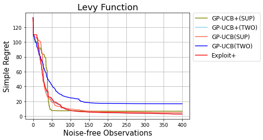
We consider three 10-dimensional benchmark objective functions: Ackley, Rastrigin, and Levy. Each of them has a unique global maximizer but many local optima, posing a challenge to standard first and second-order convex optimization algorithms. Following the virtual library of simulation experiments: https://www.sfu.ca/ ssurjano/, we respectively set the search space to be and . We used a Matérn kernel with the default initial smoothness parameter and initial lengthscale parameter . For each method and objective, we obtain 400 noise-free observations and average the results over 20 independent experiments. For GP-UCB and GP-UCB+, we set Figure 2 shows the average simple regrets, given by We report the regret as a function of the number of observations rather than the number of iterations to ensure a fair comparison. For all three benchmark functions, GP-UCB+ and EXPLOIT+ outperform the other methods. To further demonstrate the strength of the proposed algorithms, Table 1 shows the average simple regret at the last iteration, normalized so that for each benchmark objective the worst-performing algorithm has unit simple regret. Table 4 in Appendix B shows results for the standard deviation, indicating that the new methods are not only more accurate, but also more precise.
To illustrate the sensitivity of UCB algorithms to the choice of weight parameters, we include numerical results with in Appendix B. In particular, since GP-UCB+ has an additional exploration step through random sampling, using a smaller weight parameter for GP-UCB+ than for GP-UCB tends to work more effectively. Remarkably, the parameter-free EXPLOIT+ algorithm achieves competitive performance compared with UCB algorithms with well-tuned weight parameters.
| Method | Ackley | Rastrigin | Levy |
|---|---|---|---|
| GP-UCB+ | 0.222 | 0.576 | 0.146 |
| GP-UCB | 0.583 | 0.930 | 0.768 |
| EXPLOIT+ | 0.342 | 0.505 | 0.126 |
| EXPLOIT | 1.000 | 1.000 | 1.000 |
| EI | 0.832 | 0.644 | 0.142 |
| PI | 0.891 | 0.698 | 0.507 |
5.2 Random Forest Hyperparameter Tuning
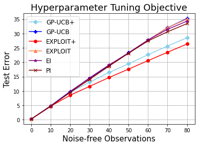
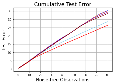
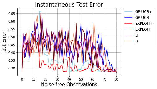
Here we use Bayesian optimization to tune four hyperparameters of a random forest regression model for the California housing dataset [19]. The parameters of interest are (i) three integer-valued quantities: the number of trees in the forest, the maximum depth of the tree, and the minimum number of samples required to split the internal node; and (ii) a real-valued quantity between zero and one: the transformed maximum number of features to consider when looking for the best split. For the discrete quantities, instead of optimizing over a discrete search space, we performed the optimization over a continuous domain and truncated the decimal values when evaluating the objective function. We split the dataset into training (80%) and testing (20%) sets. To define a deterministic objective function, we fixed the random state parameter for the RandomForestRegressor function from the Python scikit-learn package and built the model using the training set. We then defined our objective function to be the negative mean-squared test error of the built model. We used a Matérn kernel with initial smoothness parameter and initial lengthscale parameter . For the GP-UCB and GP-UCB+ algorithms, we set where consists of 40 Latin hypercube samples. We conducted 20 independent experiments with 80 noise-free observations. From Table 2 and Figure 3, we see that both GP-UCB+ and EXPLOIT+ algorithms led to smaller cumulative test errors. An instantaneous test error plot with implementation details can be found in Appendix C.
| Method | Mean SD | |
|---|---|---|
| GP-UCB+ | ||
| GP-UCB | ||
| EXPLOIT+ | ||
| EXPLOIT | ||
| EI | ||
| PI |
5.3 Garden Sprinkler Computer Model
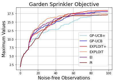
The Garden Sprinkler computer model simulates the range of a garden sprinkler that sprays water. The model contains eight physical parameters that represent vertical nozzle angle, tangential nozzle angle, nozzle profile, diameter of the sprinkler head, dynamic friction moment, static friction moment, entrance pressure, and diameter flow line. First introduced in [23] and later formulated into a deterministic black-box model by [21], the goal is to maximize the accessible range of a garden sprinkler over the domain of the eight-dimensional parameter space. In this problem, the observations of the objective are noise-free. Following [20], for GP-UCB and GP-UCB+ we set and used a squared exponential kernel with an initial lengthscale parameter . We ran 30 independent experiments, each with 100 noise-free observations. The results in Table 3 and Figure 4 demonstrate that the new algorithms achieve competitive performance. In particular, EXPLOIT+ attains on average the largest maximum value, while also retaining a moderate standard deviation across experiments.
| Method | Mean SD | |
|---|---|---|
| GP-UCB+ | 17.511 1.603 | |
| GP-UCB | 18.038 2.026 | |
| EXPLOIT+ | ||
| EXPLOIT | 17.352 2.537 | |
| EI | 18.061 1.657 | |
| PI | 17.105 2.329 |
6 Conclusion
This paper has introduced two Bayesian optimization algorithms, GP-UCB+ and EXPLOIT+, that supplement query points obtained via UCB or posterior mean maximization with query points obtained via random sampling. The additional sampling step in our algorithms promotes search space exploration and ensures that the fill-distance of the query points decays at a nearly optimal rate. From a theoretical viewpoint, we have shown that GP-UCB+ and EXPLOIT+ satisfy regret bounds that improve upon existing and refined rates for the classical GP-UCB algorithm with noise-free observations, and nearly match the rates conjectured in [31]. Indeed, at the price of a higher computational cost, one can obtain the exact rates in [31] by replacing the random sampling step in GP-UCB+ and EXPLOIT+ with a quasi-uniform sampling scheme. From an implementation viewpoint, both GP-UCB+ and EXPLOIT+ retain the appealing simplicity of the GP-UCB algorithm; moreover, EXPLOIT+ does not require specifying input weight parameters. From an empirical viewpoint, we have demonstrated that the new algorithms outperform existing ones in a wide range of examples.
References
- BCX+ [17] Somil Bansal, Roberto Calandra, Ted Xiao, Sergey Levine, and Claire J Tomlin. Goal-driven dynamics learning via Bayesian optimization. In 2017 IEEE 56th Annual Conference on Decision and Control (CDC), pages 5168–5173. IEEE, 2017.
- BK [21] Ilija Bogunovic and Andreas Krause. Misspecified Gaussian process bandit optimization. Advances in Neural Information Processing Systems, 34:3004–3015, 2021.
- BS [96] Christopher J Burges and Bernhard Schölkopf. Improving the accuracy and speed of support vector machines. Advances in Neural Information Processing Systems, 9, 1996.
- Bul [11] Adam D Bull. Convergence rates of efficient global optimization algorithms. Journal of Machine Learning Research, 12(10), 2011.
- CG [17] Sayak Ray Chowdhury and Aditya Gopalan. On kernelized multi-armed bandits. In International Conference on Machine Learning, pages 844–853. PMLR, 2017.
- CG [19] Sayak Ray Chowdhury and Aditya Gopalan. Bayesian optimization under heavy-tailed payoffs. Advances in Neural Information Processing Systems, 32, 2019.
- CJBGP [16] Daniel L Clark Jr, Ha-Rok Bae, Koorosh Gobal, and Ravi Penmetsa. Engineering design exploration using locally optimized covariance kriging. AIAA Journal, 54(10):3160–3175, 2016.
- DFSZ [12] Nando De Freitas, Alex J Smola, and Masrour Zoghi. Exponential regret bounds for Gaussian process bandits with deterministic observations. In Proceedings of the 29th International Coference on International Conference on Machine Learning, pages 955–962, 2012.
- Fra [18] Peter I Frazier. A tutorial on Bayesian optimization. arXiv preprint arXiv:1807.02811, 2018.
- GR [06] Subhashis Ghosal and Anindya Roy. Posterior consistency of Gaussian process prior for nonparametric binary regression. The Annals of Statistics, pages 2413–2429, 2006.
- HSTZ [23] Tapio Helin, Andrew M Stuart, Aretha L Teckentrup, and Konstantinos Zygalakis. Introduction to Gaussian process regression in Bayesian inverse problems, with new results on experimental design for weighted error measures. arXiv preprint arXiv:2302.04518, 2023.
- JSW [98] Donald R Jones, Matthias Schonlau, and William J Welch. Efficient global optimization of expensive black-box functions. Journal of Global optimization, 13(4):455, 1998.
- KHSS [18] Motonobu Kanagawa, Philipp Hennig, Dino Sejdinovic, and Bharath K Sriperumbudur. Gaussian processes and kernel methods: A review on connections and equivalences. arXiv preprint arXiv:1807.02582, 2018.
- KKSP [18] Kirthevasan Kandasamy, Akshay Krishnamurthy, Jeff Schneider, and Barnabás Póczos. Parallelised Bayesian optimisation via Thompson sampling. In International Conference on Artificial Intelligence and Statistics, pages 133–142. PMLR, 2018.
- KSAY [22] Hwanwoo Kim, Daniel Sanz-Alonso, and Ruiyi Yang. Optimization on manifolds via graph Gaussian processes. arXiv preprint arXiv:2210.10962, 2022.
- LYT [19] Yueming Lyu, Yuan Yuan, and Ivor W Tsang. Efficient batch black-box optimization with deterministic regret bounds. arXiv preprint arXiv:1905.10041, 2019.
- Moc [98] Jonas Mockus. The application of Bayesian methods for seeking the extremum. Towards Global Optimization, 2:117, 1998.
- OCBG [19] Chris J Oates, Jon Cockayne, François-Xavier Briol, and Mark Girolami. Convergence rates for a class of estimators based on Stein’s method. Bernoulli, 25(2):1141–1159, 2019.
- PB [97] R Kelley Pace and Ronald Barry. Sparse spatial autoregressions. Statistics & Probability Letters, 33(3):291–297, 1997.
- PL [21] Tony Pourmohamad and Herbert KH Lee. Bayesian Optimization with Application to Computer Experiments. Springer, 2021.
- Pou [20] Tony Pourmohamad. Compmodels: Pseudo computer models for optimization. R package version 0.2. 0, 2020.
- RVR [14] Daniel Russo and Benjamin Van Roy. Learning to optimize via information-directed sampling. Advances in Neural Information Processing Systems, 27, 2014.
- SHvB [10] Karl Siebertz, Thomas Hochkirchen, and D van Bebber. Statistische Versuchsplanung. Springer, 2010.
- SKKS [10] Niranjan Srinivas, Andreas Krause, Sham Kakade, and Matthias Seeger. Gaussian process optimization in the bandit setting: no regret and experimental design. In Proceedings of the 27th International Conference on Machine Learning, pages 1015–1022, 2010.
- ST [18] Andrew Stuart and Aretha Teckentrup. Posterior consistency for Gaussian process approximations of Bayesian posterior distributions. Mathematics of Computation, 87(310):721–753, 2018.
- Ste [12] Michael L Stein. Interpolation of Spatial Data: Some Theory for Kriging. Springer Science & Business Media, 2012.
- SVZ [23] Sudeep Salgia, Sattar Vakili, and Qing Zhao. Random exploration in Bayesian Optimization: order-optimal regret and computational efficiency. arXiv preprint arXiv:2310.15351, 2023.
- SY [23] Amit Singer and Ruiyi Yang. Alignment of density maps in Wasserstein distance. arXiv preprint arXiv:2305.12310, 2023.
- Tec [20] Aretha L Teckentrup. Convergence of Gaussian process regression with estimated hyper-parameters and applications in Bayesian inverse problems. SIAM/ASA Journal on Uncertainty Quantification, 8(4):1310–1337, 2020.
- TW [20] Rui Tuo and Wenjia Wang. Kriging prediction with isotropic Matérn correlations: Robustness and experimental designs. Journal of Machine Learning Research, 21(1):7604–7641, 2020.
- Vak [22] Sattar Vakili. Open problem: Regret bounds for noise-free kernel-based bandits. In Conference on Learning Theory, pages 5624–5629. PMLR, 2022.
- VKP [21] Sattar Vakili, Kia Khezeli, and Victor Picheny. On information gain and regret bounds in Gaussian process bandits. In International Conference on Artificial Intelligence and Statistics, pages 82–90. PMLR, 2021.
- Wen [04] Holger Wendland. Scattered Data Approximation, volume 17. Cambridge University Press, 2004.
- WR [06] Christopher KI Williams and Carl Edward Rasmussen. Gaussian Processes for Machine Learning, volume 2. MIT Press Cambridge, MA, 2006.
- WS [93] Zong-min Wu and Robert Schaback. Local error estimates for radial basis function interpolation of scattered data. IMA Journal of Numerical Analysis, 13(1):13–27, 1993.
- WSH [21] Tizian Wenzel, Gabriele Santin, and Bernard Haasdonk. A novel class of stabilized greedy kernel approximation algorithms: Convergence, stability and uniform point distribution. Journal of Approximation Theory, 262:105508, 2021.
- WTJW [20] Wenjia Wang, Rui Tuo, and CF Jeff Wu. On prediction properties of kriging: Uniform error bounds and robustness. Journal of the American Statistical Association, 115(530):920–930, 2020.
Appendix A Proofs
Proof of Theorem 3.1.
Let and let be the instantaneous regret. Then,
| (A.1) | ||||
where for (i) we use twice that, for any it holds that —see for instance Corollary 3.11 in [13]— and for (ii) we use the definition of in the GP-UCB algorithm. Thus, for any
where (i) follows by the Cauchy-Schwarz inequality, (ii) from the bound on , and (iii) from the fact that for any . Since the function is strictly increasing in and for the squared exponential kernel it holds that we have that Therefore,
| (A.2) |
where the last inequality follows from Lemma 5.3 in [24]. Since (A.2) holds for any , by plugging , for some , we conclude that
| (A.3) |
For squared exponential kernels, Corollary 1 in [32] implies that
where is independent of and Hence, using that for , we obtain
concluding the proof. ∎
Proof of Theorem 4.4.
We first prove the cumulative regret bound for GP-UCB+. As in (A.1), one can show that
For Matérn kernels, [35] shows that —see also Lemma 2 in [37]. Moreover, we have the trivial bound Hence, for any
where follows from Proposition 4 in [11] —see also Lemma 2 in [18].
For squared exponential kernels, Theorem 11.22 in [33] shows that, for some Hence, for any ,
where follows from Proposition 4 in [11] —see also Lemma 2 in [18]. Since , we conclude that .
For the EXPLOIT+ algorithm, we have that
where for (i) we use twice that, for any it holds that and for (ii) we use the definition of in the EXPLOIT+ algorithm. The rest of the proof proceeds exactly as the one for GP-UCB+, and we hence omit the details. ∎
Proof of Theorem 4.8.
By Lemma 5.5 in [24], the choice of in the statement of Theorem 4.8 ensures that, with probability at least
Furthermore, Lemma 5.7 in [24] implies that, with probability at least
where is the point in closest to and is a discretization of size inside satisfying that, for all
For the GP-UCB+ algorithm,
where (i) follows from Lemma 5.7 in [24], (ii) from the definition of in the GP-UCB+ algorithm, and (iii) from Lemma 5.5 in [24]. Therefore, with probability at least
from which we deduce that
Using the same argument as in the proof of Theorem 4.4 and the choice of , we obtain the desired result.
Appendix B Additional Experiments and Implementation Details: Benchmark Functions
This appendix provides detailed descriptions of the numerical experiments conducted in Section 5.1. The functional forms of the three objective functions we considered and their respective search space are provided below. For all three benchmark functions we denote and set
-
•
Ackley function:
-
•
Rastrigin function:
-
•
Levy function: With , for all
| Method | Ackley | Rastrigin | Levy |
|---|---|---|---|
| GP-UCB+ | 0.075 | 0.797 | 0.131 |
| GP-UCB | 1.000 | 1.000 | 0.719 |
| EXPLOIT+ | 0.306 | 0.577 | 0.127 |
| EXPLOIT | 0.733 | 0.976 | 1.000 |
| EI | 0.466 | 0.609 | 0.160 |
| PI | 0.329 | 0.360 | 0.312 |
Recall that Figure 2 portrayed the average simple regret of the six Bayesian optimization strategies we consider: GP-UCB+ (proposed algorithm), GP-UCB ([24]) (both with the choice of ), EXPLOIT+ (proposed algorithm), EXPLOIT (GP-UCB with ), EI (Expected Improvement), and PI (Probability of Improvement). The simple regret values at the last iteration were displayed in Table 1. Furthermore, Table 4 shows the standard deviations of the last simple regret values over 20 independent experiments. From Figure 2 and Table 4, one can see that not only were the proposed methods (GP-UCB+ and EXPLOIT+) able to yield superior simple regret performance, but also their standard deviations were substantially smaller than those of the other methods, indicating superior stability.
Additionally, Figure 5 shows the cumulative regret for GP-UCB+ and GP-UCB with different choices of . All results were averaged over 20 independent experiments. We considered and where is a set of 100 Latin hypercube samples. In all experiments, was significantly larger than . Figure 5 demonstrates that the choice of can significantly influence the cumulative regret. In particular, we have observed that the GP-UCB+ algorithm tends to work better with smaller values, as the algorithm contains additional exploration steps through random sampling; this behavior can also be seen in Figure 5. In all three benchmark functions, GP-UCB exhibits sensitivity to the choice of parameter ; in contrast, our EXPLOIT+ algorithm does not require specifying weight parameters and consistently achieves competitive or improved performance across all our experiments.
Appendix C Additional Figures and Implementation Details: Hyperparameter Tuning
To train the random forest regression model for California housing dataset [19], we first divided the dataset into test and train datasets. 80 percent of (feature vector, response) pairs were assigned to be the training set, while the remaining 20 percent were treated as a test set. In constructing the deterministic objective function, we defined it to be a mapping from the vector of four hyperparameters to a negative test error of the model built based on the input and training set. As the model construction may involve randomness coming from the bootstrapped samples, we fixed the random state parameter to remove any such randomness in the definition of the objective. We tuned the following four hyperparameters:
-
•
Number of trees in the forest
-
•
Maximum depth of the tree
-
•
Minimum number of samples requires to split the internal node
-
•
Maximum proportion of the number of features to consider when looking for the best split
For the first three parameters we conducted the optimization task in the continuous domain and rounded down to the nearest integers. Figure 6 shows that the proposed algorithms attained smaller cumulative and instantaneous test errors.
Appendix D Implementation Details: Garden Sprinkler Computer Model
For the Garden Sprinkler computer model, the eight-dimensional search space we considered was given by:
-
•
Vertical nozzle angle
-
•
Tangential nozzle angle
-
•
Nozzle profile
-
•
Diameter of the sprinkler head
-
•
Dynamic friction moment
-
•
Static friction moment
-
•
Entrance pressure
-
•
Diameter flow line