Optimal Potential Shaping on SE(3) via Neural ODEs on Lie Groups

Abstract

This work presents a novel approach for the optimization of dynamic systems on finite-dimensional Lie groups. We rephrase dynamic systems as so-called neural ordinary differential equations (neural ODEs), and formulate the optimization problem on Lie groups. A gradient descent optimization algorithm is presented to tackle the optimization numerically. Our algorithm is scalable, and applicable to any finite dimensional Lie group, including matrix Lie groups. By representing the system at the Lie algebra level, we reduce the computational cost of the gradient computation. In an extensive example, optimal potential energy shaping for control of a rigid body is treated. The optimal control problem is phrased as an optimization of a neural ODE on the Lie group $SE(3)$, and the controller is iteratively optimized. The final controller is validated on a state-regulation task.

1 Introduction

Many physical systems are naturally described by the action of Lie groups on their configuration manifolds. This can range from finite-dimensional systems such as rigid bodies, where poses are acted on by the special Euclidean group $SE(3)$ Murray1994 , towards infinite-dimensional systems such as flexible bodies or fluid dynamical systems, where the diffeomorphism group acts on the configuration of the continuum Schmid2010 .

Geometric control systems on Lie groups Brockett1973 Jurdjevic1996 exploit the Lie group structure of the underlying physical systems to provide numerical advantages Marsden1999 . For example, PD controllers for rigid bodies were defined on $SO(3)$ and $SE(3)$ by Bullo & Murray in bullo_murray_1995 , and more recently geometric controllers were applied in the context of UAV’s Lee2010 Goodarzi2013 Rashad2019 . Examples for efficient optimal control formulations on Lie groups include linear Ayala2021 and nonlinear systems Spindler1998 , as well as efficient numerical optimization methods Kobilarov2011 Saccon2013 Teng2022 .

In an orthogonal development over the recent years, there has been a surge of machine learning applications in control Dev_ML_Control_Review_2021 and robotics Taylor2021 Ibarz2021 Soori_AI_Robotics_Review_2023 . This surge is driven by the need for controllers that work in high-dimensional robotic systems and approximate complex decision policies that require the use of data. The implementation of such controllers through classical control theoretic approaches is prohibitive, and it led to a paradigm shift towards data-driven control Taylor2021 . Examples of machine learning within high-dimensional systems extend to soft robotics Kim_ML_Soft_Robotics_Review_2021 and control of fluid systems paris_RL_flow_control_2021 . The literature also aims to address common concerns of safety Hewing2020 Brunke2022 both during the training process and in the deployment of systems with machine learning in the loop.

The so-called Erlangen program of machine learning by Bronstein et al. Bronstein2021 stresses the importance of geometric machine learning methods: symmetries of data sets can restrict the complexity of functions that are to be learned on them, and thus increase the numerical efficiency of learning frameworks. This rationale also led to extensions of machine learning approaches to Lie groups Fanzhang2019 Lu2020 , with recent applications in Huang2017 Chen2021 Forestano2023 .

Indeed, the fundamental symmetry groups in robotics are naturally represented by Lie groups Marsden1999 . As such, Lie group-based learning methods are of interest to the robotics community. In an excellent example of a control application Duong et al. Duong2021_nODE_SE3 extended neural ODEs to $SE(3)$ and applied it to the adaptive control of a UAV in Duong2021_Adaptive_control_via_nODE_SE3 .

However, a general approach for geometric machine learning in the context of dynamic systems on Lie groups is missing. We believe that such an approach would be of high interest, especially for control applications. In this paper, we address this issue by formalizing neural ODEs on Lie groups.

Our contributions are 1.: the formulation of neural ODEs on any finite-dimensional Lie group, with a particular focus on matrix Lie groups; 2.: various computational simplifications related to the computation of gradients and second gradients on Lie groups and a reduced need for chart switches by moving sensitivity computations to the Lie algebra level; 3.: a pytorch & torchdyn compatible algorithm for the optimization of a general potential energy shaping and damping injection control on $SE(3)$, for which stability is implemented as a design requirement; 4.: the formulation of a minimal exponential Atlas on the Lie group $SE(3)$.

The article is divided into two parts: first the formulation of neural ODEs on finite-dimensional matrix Lie groups, and second an extensive example of optimal potential energy shaping on $SE(3)$.

Section 2 presents the main technical contribution of the article: the generalized adjoint method on Lie groups, which is at the heart of a gradient descent algorithm for dynamics optimization via neural ODEs on Lie groups.

A number of technical tools are required to apply this algorithm on a given matrix Lie group, which are introduced in Section 3. The exponential Atlas allows to implement a numerical procedure for exact integration on Lie groups, while a compact formula for the gradient of a function on a Lie group reduces complexity of the gradient computation.

Section 4 presents the Lie groups $SO(3)$ and $SE(3)$, and gives concrete examples of the technical tools presented in the previous section. One aspect of this is the formulation of a minimal exponential Atlas on $SE(3)$, which is used to formulate an integration procedure on $SE(3)$. This treatment prepares the stage for control optimization of a rigid body on $SE(3)$.

Section 5 introduces the example of optimizing potential energy and damping injection controllers for rigid bodies on $SE(3)$. The class of controllers is defined and it is shown that it guarantees stability by design. Afterwards, the optimization of a cost-functional over the defined class of controllers is derived from the general procedure in Section 2.

Finally, Section 6 provides two examples of optimizing controllers for a rigid body on $SE(3)$. The first example concerns pose control, without gravity, and results are compared to a quadratic controller of the type presented by Rashad2019 . In the second example, the controller’s performance is investigated in the presence of gravity.

The article ends with a discussion in Section 7 and a conclusion in Section 8.

1.1 Neural ODEs and relation to existing works

Neural ODEs were first introduced by Chen et al. chen2019neural , who derived them as the continuous limit of recurrent neural nets, taking inputs on $\mathbb{R}^{n}$. Their cost functionals only admitted intermediate and final cost terms, for which they showed that the so-called adjoint method allows a memory-efficient computation of the gradient.

Massaroli et al. Massaroli2021 introduced a more general framework of neural ODEs, showing the power of state-augmentation and connections to optimal control, while also showing that the cost functional can include integral cost terms. To this end, they presented the generalized adjoint method.

There are two highly relevant examples in the recent literature that extend neural ODEs to manifolds. The so-called extrinsic picture is presented by Falorsi et al. Falorsi2020 , who show that neural ODEs on a manifold $\mathcal{M}$ can be optimized as classical neural ODEs on an embedding $\mathbb{R}^{n}$. Given an extension of the manifold neural ODE to $\mathbb{R}^{n}$, they show that the adjoint method on $\mathbb{R}^{n}$ can be applied for optimization of the manifold neural ODE.

An intrinsic picture is presented by Lou et al. Lou2020 , who show that neural ODEs on a manifold $\mathcal{M}$ can be expressed in local charts on the manifold, where the adjoint method holds locally. They use exponential charts on Riemannian manifolds, and achieve a dimensionality-reduction and geometric exactness with respect to Falorsi et al. Both Falorsi2020 and Lou2020 carefully extend neural ODEs to manifolds, and consider neural ODE on Lie groups to be a sub-class of the presented manifold neural ODEs. With respect to their work, we show how to include integral costs in a generalized adjoint method on manifolds and Lie groups, and show the advantages of considering neural ODEs on Lie groups as a specialized class of algorithms.

An example of neural ODEs to control of robotic systems described on $\mathbb{R}^{n}$ is described in Massaroli2020 , where an IDA-PBC controller is optimized.

Duong et al. Duong2021_nODE_SE3 Duong2021_Adaptive_control_via_nODE_SE3 apply neural ODEs to control optimization for a rigid body on $SE(3)$. The work focuses on the formulation of an IDA-PBC controller, uses it for dynamics learning and trajectory tracking, and uses neural ODEs as a tool for this optimization. While the integration procedure used is not geometrically exact and the Lie group constraints are violated, the approach is highly successful. However, Duong et al. do not connect their contribution to geometric machine learning literature such as neural ODEs on manifolds. With respect to Duong et al., we present the general picture of neural ODEs on Lie groups. By extending the intrinsic formulation to Lie groups, our example on $SE(3)$ has a reduced number of dimensions (24 instead of 36), and the use of local charts allows geometrically exact integration.

1.2 Notation

While the main results are accessible with a background of linear algebra and vector calculus, the derivations heavily rely on differential geometry and Lie group theory, see e.g, Isham1999 and Hall2015 for a complete introduction, or sola2021micro for a brief introduction with examples in robotics.

Calligraphic letters $\mathcal{M},\,\mathcal{N},\,\mathcal{U},\,\mathcal{P}$ denote smooth manifolds. Respectively, $T_{x}\mathcal{M}$ and $T_{x}^{*}\mathcal{M}$ denote the tangent and cotangent space at $x\in\mathcal{M}$, $T\mathcal{M}$ and $T^{*}\mathcal{M}$ denote the tangent bundle and cotangent bundle of $\mathcal{M}$, and $\Gamma(T\mathcal{M})$ and $\Gamma(T^{*}\mathcal{M})$ are the sets of sections that collect vector fields and co-vector fields over $\mathcal{M}$. Curves $x:\mathbb{R}\rightarrow\mathcal{M}$ are evaluated as $x(t)$, and their tangent vectors are denoted as $\dot{x}\in T_{x(t)}\mathcal{M}$.

Upper case letters $G,H$ denote Lie groups, while lower case letters $g,h$ denote their elements. A lower case $e$ denotes the group identity $e\in G$, an upper case $I$ denotes the identity matrix. The Lie algebra is $\mathfrak{g}$, and its dual is $\mathfrak{g}^{*}$. Letters $\tilde{A},\tilde{B}$ denote vectors in the Lie algebra, while letters $A,B$ denote vectors in $\mathbb{R}^{n}$.

Furthermore $C^{k}(\mathcal{M},\mathcal{N})$ denotes the set of continuous, $k$-times differentiable functions between $\mathcal{M}$ and $\mathcal{N}$. For $\phi\in C^{k}(\mathcal{M},\mathcal{N})$, let $\phi_{*}:\Gamma(T\mathcal{M})\rightarrow\Gamma(T\mathcal{N})$ and $\phi^{*}:\Gamma(T^{*}\mathcal{N})\rightarrow\Gamma(T^{*}\mathcal{M})$ denote the push-forward and pullback, respectively.

For $V\in C^{1}(\mathcal{M},\mathbb{R})$, let $\text{d}V\in\Gamma(T^{*}\mathcal{M})$ denote the gradient co-vector field. When $\mathcal{M}=\mathbb{R}^{k}$, the gradient at $x\in\mathbb{R}^{k}$ is denoted by $\frac{\partial V}{\partial x}\in\mathbb{R}^{k}$.

When coordinate expressions are concerned, the Einstein summation convention is used, i.e., the product of variables with lower and upper indices implies a sum $a_{i}b^{i}:=\sum_{i}a_{i}b^{i}$.

Let $(X,D,\mathbb{P})$ denote a probability space with $X$ a topological space, $D$ the Borel $\sigma$-algebra and $\mathbb{P}:D\rightarrow[0,1]$ a probability measure. Given a vector space $L$ and a random variable $C:X\rightarrow L$, denote by $\mathbb{E}_{x\sim\mathbb{P}}(C):=\int_{X}C(x)\text{d}\mathbb{P}(x)$ the expectation of $C$ w.r.t. $\mathbb{P}$.

2 Main Result

After a brief introduction to Lie groups in Section 2.1, the optimization problem is introduced on abstract Lie groups in Section 2.2. A gradient descent optimization algorithm is presented in Section 2.3. Our main technical result, the generalized adjoint method on Lie groups, lies at the core of the gradient computation. For the sake of exposition, we present it in the context of matrix Lie groups, and relegate the derivations and the formulation on abstract Lie groups to Appendix A.4.

2.1 Lie groups

A finite-dimensional Lie group $G$ is an $n$-dimensional manifold together with a group structure, such that the group operation is a smooth map on $G$ Isham1999 . $G$ is a real matrix Lie group if it is a subgroup of the general linear group $GL(m,\mathbb{R})$

$$GL(m,\mathbb{R}):=\{g\in\mathbb{R}^{m\times m}\;|\;\text{det}(g)\neq 0\}\,,$$ (1)

where the group operation for a matrix Lie group is given by matrix multiplication Hall2015 . For $g,h\in G$ the left translation by $h$ is defined as

$$L_{h}:G\rightarrow G\,;\;L_{h}(g):=hg\,.$$ (2)

We denote the Lie algebra of $G$ as $\mathfrak{g}:=T_{e}G$, and its dual as $\mathfrak{g}^{*}:=T^{*}_{e}G$.

Define a basis $E:=\{\tilde{E}_{1},\ldots,\tilde{E}_{n}\}$ with $\tilde{E}_{i}\in\mathfrak{g}$, and define the (invertible, linear) map $\Lambda:\mathbb{R}^{n}\rightarrow\mathfrak{g}$ as

$$\Lambda:\mathbb{R}^{n}\rightarrow\mathfrak{g}\,;\;(x^{1},\ldots,x^{n})\mapsto\sum_{i}x^{i}\tilde{E}_{i}\,.$$ (3)

The dual of $\Lambda$ is the map $\Lambda^{*}:\mathfrak{g}^{*}\rightarrow\mathbb{R}^{n}$. Define the dual basis $\{\bar{E}^{1},\ldots,\bar{E}^{n}\}$ with $\bar{E}^{i}\in\mathfrak{g}^{*}$ by $\bar{E}^{i}(\tilde{E}_{j})=\delta_{j}^{i}$ with $\delta_{j}^{i}$ the Kronecker delta. Then ${\Lambda^{*}}^{-1}$ is explicitly given by

$${\Lambda^{*}}^{-1}:\mathbb{R}^{n}\rightarrow\mathfrak{g}^{*}\,;\;(x_{1},\ldots,x_{n})\mapsto\sum_{i}x_{i}\bar{E}^{i}\,.$$ (4)

For a matrix Lie group the Lie algebra $\mathfrak{g}$ is a subspace of the Lie algebra $gl(m,\mathbb{R})$ of $GL(m,\mathbb{R})$. Here $gl(m,\mathbb{R})$ is defined as

$$gl(m,\mathbb{R}):=\mathbb{R}^{m\times m}\,.$$ (5)

For $\tilde{A},\tilde{B}\in\mathfrak{g}$ the adjoint map $\text{ad}_{\tilde{A}}(\tilde{B})$ is a bilinear map defined in terms of the (left) Lie bracket

$$\text{ad}:\mathfrak{g}\times\mathfrak{g}\rightarrow\mathfrak{g}\,;\;\text{ad}_{\tilde{A}}(\tilde{B})=\tilde{A}\tilde{B}-\tilde{B}\tilde{A}\,.$$ (6)

Using the operator $\Lambda$, a matrix representation of ad is obtained as $\Lambda^{-1}\big{(}\text{ad}_{\Lambda(A)}\Lambda(\cdot)\big{)}\in\mathbb{R}^{n\times n}$, called the adjoint representation. By an abuse of notation, we denote the adjoint representation as $\text{ad}_{A}$, without a tilde in the subscript.

On matrix Lie groups and for functions $V\in C^{1}(G,\mathbb{R})$ the gradient $\text{d}_{g}V\in\mathbb{R}^{n}$ (see Section 3.4 for details) is found as:

$$\text{d}_{g}V=\frac{\partial}{\partial q}V\bigg{(}g\big{(}I+\Lambda(q)\big{)}\bigg{)}_{|q=0}\,.$$ (7)

2.2 Optimization problem

We consider a variant of the optimal control problem on a Lie group Jurdjevic1996 with a finite horizon $T$. Given parameters $\theta\in\mathbb{R}^{n_{\theta}}$, denote the parameterized dynamics on a Lie group as $f_{\theta}(g,t):=f(g,t,\theta)$. Then, given the dynamic system

$$\dot{g}=f_{\theta}(g,t)\,,\;g(0)=g_{0}\,,$$ (8)

denote the solution operator (also called the flow) as

$$\Psi^{t}_{f_{\theta}}:G\rightarrow G\,;\;g(0)\mapsto g(t)\,,$$ (9)

and define the real valued cost function

$$C^{T}_{f_{\theta}}(g_{0},\theta)=F(\Psi^{T}_{f_{\theta}}(g_{0}),\theta)+\int_{0}^{T}r(\Psi^{s}_{f_{\theta}}(g_{0}),\theta,s)\text{d}s\,,$$ (10)

where we call $F$ the final cost term and $r$ the running cost term.

Indicating a probability space $(G,D,\mathbb{P})$, we are interested in solving the minimization problem

$$\min_{\theta}\; \mathbb{E}_{g_{0}\sim\mathbb{P}}C^{T}_{f_{\theta}}(g_{0},\theta)\,.$$ (11)

Remark 2.1.

The chief reason for our interest in this optimization problem is that it includes, as a subclass, the optimization of state-feedbacks $u_{\theta}:G\times[0,T]\rightarrow\mathcal{U}$ by considering dynamics of the form $f(g,t,u_{\theta}(g,t))$, where $u_{\theta}$ denotes the control input of the system.

Remark 2.2.

The dynamics $f_{\theta}(g,t)$ can also be parameterized with neural nets, in which case $f_{\theta}(g,t)$ is referred to as a neural ODE on a Lie group. Indeed, for the Lie group $(\mathbb{R}^{n},+)$, the formulation agrees with the definition of a neural ODE given in Massaroli2021 who define them as dynamics $\dot{x}=f_{\theta}(x,t)$ with $x\in\mathbb{R}^{n}$.

2.3 Optimization algorithm

We use a stochastic gradient descent optimization algorithm Robbins1951 to approximate a solution to the optimization problem (11) on a matrix Lie group.

Denote the total cost in (11) as

$$J(\theta):=\mathbb{E}_{g_{0}\sim\mathbb{P}}C^{T}_{f_{\theta}}(g_{0},\theta)\,.$$ (12)

Additionally, denote by $\theta_{k}\in\mathbb{R}^{n_{\theta}}$ the parameters at the $k$-th iteration, and by $\eta_{k}$ a positive scalar learning rate at the $k$-th iteration. Then a standard gradient descent algorithm computes the parameters $\theta_{k+1}$ by an application of the update rule

$$\theta_{k+1}=\theta_{k}-\eta_{k}\frac{\partial}{\partial\theta}J(\theta)\,.$$ (13)

In stochastic gradient descent $N$ initial conditions $g_{i}$ are sampled from the probability distribution corresponding to the probability measure $\mathbb{P}$. The expectation in (13) is approximated by averaging the gradients of costs $C_{i}=C^{T}_{f_{\theta}}(g_{i},\theta)$ of the individual trajectories starting at $g_{i}$ as

$$\frac{\partial}{\partial\theta}J(\theta)=\mathbb{E}_{g_{0}\sim\mathbb{P}}\frac{\partial}{\partial\theta}C^{T}_{f_{\theta}}(g_{0})\approx\frac{1}{N}\sum_{i=0}^{N}\frac{\partial}{\partial\theta}C_{i}\,.$$ (14)

For convex cost-functions $J(\theta)$ and a sufficiently small $\eta_{k}$, the parameter $\theta_{k}$ approaches the optimal parameters $\theta^{\star}$ as $k$ increases Robbins1951 . For non-convex cost-functions stochastic gradient descent does not have a guarantee of global optimality, but it is still widely used as a light and scalable algorithm ruder2017overview that results in robust local optima xie2021diffusion .

In order to compute the gradient $\frac{\partial}{\partial\theta}C_{i}$ of the cost for a single trajectory (10), we derived the generalized adjoint method on matrix Lie groups. It is the main technical result of this paper, and it is stated in the following:

Theorem 2.1 (Generalized Adjoint Method on Matrix Lie Groups).

Given are the dynamics (8) and the cost (10). Denote by $\tilde{f}_{\theta}(g,t):=g^{-1}f_{\theta}(g,t)\in\mathfrak{g}$. Then the parameter gradient $\frac{\partial}{\partial\theta}C^{T}_{f_{\theta}}(g_{0})$ of the cost is given by the integral equation

$$\frac{\partial}{\partial\theta}C^{T}_{f_{\theta}}(g_{0})=\frac{\partial F}{\partial\theta}+\int_{0}^{T}\frac{\partial}{\partial\theta}\big{(}\lambda_{g}^{\top}\Lambda^{-1}(\tilde{f}_{\theta})\big{)}+\frac{\partial r}{\partial\theta}\text{d}t\,,$$ (15)

where the state $g(t)\in G$ and adjoint state $\lambda_{g}(t)\in\mathbb{R}^{n}$ are the solutions of the system of equations

$$\dot{g} =f_{\theta}\,,\;g(0)=g_{0}\,,$$ (16)

$$\dot{\lambda}_{g} =-\text{d}_{g}\big{(}\lambda_{g}^{\top}\Lambda^{-1}(\tilde{f}_{\theta})+r\big{)}+\text{ad}_{\tilde{f}_{\theta}}^{\top}\lambda_{g}\,,\;\lambda_{g}(T)=\text{d}_{g}F\,.$$ (17)

Proof.

For a derivation of Theorem 2.1 via neural ODEs on manifolds, refer to Appendix A. ∎

The generalized adjoint methodMassaroli2021 on $\mathbb{R}^{n}$ is recovered as a special case for the Lie group $(\mathbb{R}^{n},+)$, for which the adjoint term $\text{ad}_{T}=0$ such that equation (17) agrees with the adjoint equation on $\mathbb{R}^{n}$.

Just as the generalized adjoint method on $\mathbb{R}^{n}$, the generalized adjoint method on Lie groups has a constant memory efficiency with respect to the network depth $T$. This makes it an advantageous choice for the gradient computation compared to e.g., back-propagation through an ODE solver.

Various technical tools are required to apply Theorem 2.1 in practice. This includes the exponential Atlas for exact integration of $\dot{g}$, a tractable expression of the gradient operator $\text{d}_{g}:C^{1}(G,\mathbb{R})\rightarrow\mathbb{R}^{n}$, and the composition of matrix Lie groups to create new matrix Lie groups from old ones. These tools are the subject of Section 3.

Remark 2.3.

Equations (16) and (17) are solved by integrating (16) forward in time, computing $\text{d}_{g}F$ at $g=g(T)$, and integrating (17) backwards in time, reusing $g(t)$ from the forward integration.

Remark 2.4.

The choice of group action for $(\mathbb{R}^{n},\bullet)$ plays an important role in recovering the adjoint equation on $\mathbb{R}^{n}$. This choice is a nontrivial degree of freedom of the optimization (see also Remark 5.3).

3 Technical Tools

A number of technical tools are presented in the context of matrix Lie groups. Given mild adaptations of the definitions these tools also apply to abstract finite-dimensional Lie groups (see Appendix A.4).

3.1 Atlas and minimal Atlas on Lie groups

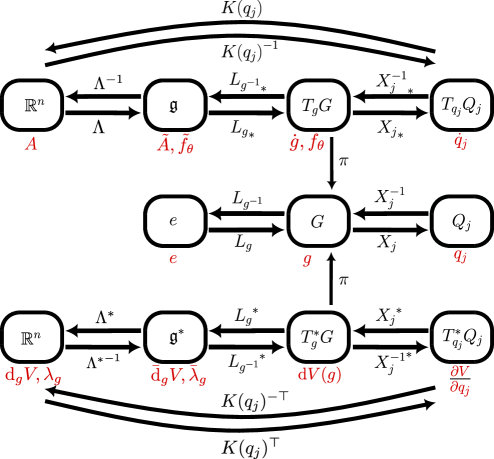
Figure 1: Commutative diagram of a generic Lie group $G$. Boxes represent sets, while arrows represent functions between sets. Relevant variables in a given set are indicated in red.

In this section the exponential map and logarithmic maps will be used to construct an atlas of exponential charts for finite-dimensional Lie groups, and the concept of a minimal exponential atlas will be defined. Here an atlas is defined as follows:

Definition 3.1 (Atlas and Charts).

An atlas $\mathcal{A}$ for an $n$-dimensional smooth manifold $\mathcal{M}$ is a collection of charts $(U,X)$, where $U\subseteq\mathcal{M}$ is an open set, $X:U\rightarrow\mathbb{R}^{n}$ is a diffeomorphism called a chart map, and the chart domains satisfy $\bigcup_{(U,X)\in\mathcal{A}}U=\mathcal{M}$.

For finite-dimensional Lie groups the exponential map $\exp:\mathfrak{g}\rightarrow G$ is a local diffeomorphism (Isham1999 , Chapter 4.2.3). Its inverse $\log:U\rightarrow\mathfrak{g}$ is defined by $\log\circ\exp=\text{id}_{U}$, for a neighborhood $U$ of the identity $e\in G$, and $\text{id}_{U}$ is the identity map on $U$.

For a matrix Lie group, the exponential map is given by the infinite sum (Hall2015 , Chapter 3.7):

$$\exp(\tilde{A}):=\sum_{n=0}^{\infty}\frac{1}{n!}\tilde{A}^{n}\,.$$ (18)

Conversely, the $\log$ map for matrix Lie groups is given by the matrix logarithm, when it is well-defined (Hall2015 , Chapter 2.3):

$$\log(g)=\sum_{n=1}^{\infty}(-1)^{n+1}\frac{(g-I)^{n}}{n}\,.$$ (19)

On a case-by-case basis the infinite sums in (18) and (19) can further be reduced to a finite sum by use of the Cayley-Hamilton Theorem Visser2006 , which often allows one to find a closed-form expression of the $\exp$ and $\log$ maps.

The logarithmic map (19) and $\Lambda$ in equation (3) can then be used to construct a local exponential chart $(U,X)$ for $G$, where

$$X:\, U\rightarrow\mathbb{R}^{n}\,;\;g\mapsto\Lambda^{-1}\log(g)\,,$$ (20)

assigns so-called coordinates $q\in\mathbb{R}^{n}$ to group elements $g\in U\subseteq G$, with the zero coordinates assigned to the group identity $e$.

To create a chart “centered” on any $h\in G$ (i.e. the zero coordinates are assigned to $h$), both the region $U$ and the chart map $X$ can be left-translated by $L_{h}$ to define the chart $(U_{h},X_{h})$ with

$$U_{h} =\,\{hg\;|\;g\in U\}\,,$$ (21)

$$X_{h} :\,U_{h}\rightarrow\mathbb{R}^{n}\,;\;g\mapsto\Lambda^{-1}\log(h^{-1}g)\,,$$ (22)

$$X_{h}^{-1} :\,\mathbb{R}^{n}\rightarrow U_{h}\,;\;q\mapsto h\exp\big{(}\Lambda({q})\big{)}\,.$$ (23)

The collection $\mathcal{A}$ of charts $(U_{h},X_{h})$ is then called an exponential atlas. This atlas covers the Lie group $G$, and is fully determined by the choice of basis $E\subset\mathfrak{g}$ and chart region $U\subset G$.

In order to use a finite number of charts, we are interested in constructing a minimal exponential atlas. A minimal atlas is defined as follows:

Definition 3.2 (Minimal Atlas).

An atlas $\mathcal{A}$ is minimal if it covers the manifold, i.e. $\mathcal{M}=\bigcup_{(U,X)\in\mathcal{A}}U$, and if it does so with the minimum number of charts.

Remark 3.1.

Given a manifold $\mathcal{M}$, the size of a minimal atlas is determined by a topological invariant, the integer $\text{Cat}(\mathcal{M})$ (the Lusternik-Schnirrelmann category, see Oprea2014 Grafarend2011 ). Given a Lie group $G$, $\text{Cat}(G)$ provides a lower bound on the size of a minimal exponential atlas.

Remark 3.2.

Given a minimal exponential atlas (which can be seen to be always countable) we use integers $j$ to number the relevant chart-centers as $g_{j}$, the corresponding charts as $(U_{j},X_{j})$, and denote the chart-coordinates in the $j$-th chart as $q_{j}\in\mathbb{R}^{n}$.

3.2 Vectors on Lie groups

Given a curve $g:\mathbb{R}\rightarrow G$ and its coordinate representation $q_{j}(t)=X_{j}(g(t))$ through (22), one can relate the tangent-vector $\dot{q}_{j}\in T_{q_{j}}Q_{j}$ of $q_{j}\in Q_{j}\subseteq\mathbb{R}^{n}$ to an element $\tilde{A}\in\mathfrak{g}$, and further to an element $A=\Lambda^{-1}(\tilde{A})\in\mathbb{R}^{n}$ (see Fig. 1) by

$$A=K(q_{j})\dot{q}_{j}\,.$$ (24)

The map $K:\mathbb{R}^{n}\rightarrow\mathbb{R}^{n\times n}$ is called the derivative of the exponential map, and it is given by the power series rossmann2006lie

$$K(q_{j})=\sum_{k=0}^{\infty}\frac{(-1)^{k}}{(k+1)!}\text{ad}_{q_{j}}^{k}\,.$$ (25)

Recall that $\text{ad}_{q_{j}}$ is an $n$-by-$n$ matrix, and $\text{ad}_{q_{j}}^{k}$ is the $k$-th power of such matrices. As with the matrix exponential (18), the infinite sum can then be reduced to a finite sum by use of the Cayley-Hamilton Theorem Visser2006 .

Remark 3.3.

The expression (24) is invariant under choice of exponential chart, i.e., for any charts $(U_{j},X_{j})$ and $(U_{k},X_{k})$ one has that $K(q_{j})\dot{q}_{j}=K(q_{k})\dot{q}_{k}$ (see Appendix B.1).

3.3 Lie group integrators

We adapt the Runge-Kutta-Munthe-Kaas (RKMK) method MuntheKaas1999 for exact integration of the dynamics (8). The RKMK method uses the Runge-Kutta scheme on Lie groups - we instead allow for arbitrary numerical integration schemes. For an overview of Lie group integrators, see e.g. iserles_2000 Celledoni_2014 Celledoni_2003 .

Using equation (24), the dynamics (8) can be represented in a local exponential chart as Celledoni_2014

$$\dot{q}_{j}=K(q_{j})^{-1}f_{\theta}\big{(}X_{j}^{-1}(q_{j}),t\big{)}\,.$$ (26)

An arbitrary numerical integration scheme can then be used to integrate the dynamics, as long as the state $q_{j}$ remains in the chart region $U_{j}$.

To make sure the state remains within the chart region we switch charts when needed by application of

$$q_{i}=X_{i}\big{(}X_{j}^{-1}(q_{j})\big{)}\,.$$ (27)

Here the conditions for chart switches are a degree of freedom. It is possible to always choose the chart $(X_{h},U_{h})$ with $h=X_{j}^{-1}\big{(}q_{j}(t)\big{)}$, i.e., to switch charts after every step of the numerical integrator (see MuntheKaas1999 Celledoni_2014 ).

Given a minimal exponential atlas, we choose to reduce the amount of chart switches. To this end, we introduce indicator functions $\sigma_{j}:G\rightarrow\mathbb{R}$ s.t. $\sigma_{j}(g)>0$ if $g\in U_{j}$, and switch charts when $\sigma_{j}(g)$ is smaller than a threshold value (see Appendix B.2).

3.4 Gradients on Lie groups

The gradient of a function $V\in C^{1}(G,\mathbb{R})$ is the co-vector field $\text{d}V\in\Gamma(TG)$. For any given $g\in G$ the gradient $\text{d}V(g)\in T_{g}^{*}G$ is a co-vector, and transforms in a dual manner to a vector $\dot{g}\in T_{g}G$. With reference to Figure 1, the gradient can be represented as

$$\bar{\text{d}}_{g}V:=(L_{g})^{*}\text{d}V(g)\in\mathfrak{g}^{*}\,,$$ (28)

and as

$$\text{d}_{g}V:={\Lambda^{*}}(\bar{\text{d}}_{g}V)\in\mathbb{R}^{n}\,.$$ (29)

Equivalently, $\text{d}_{g}V$ can be found from the computation in a chart $(U_{j},X_{j})$ as (indeed, dual to (24))

$$\text{d}_{g}V=K(q_{j})^{-\top}\frac{\partial V}{\partial q_{j}}_{|q_{j}=X_{j}(g)}\,.$$ (30)

Here, a computationally advantageous choice can be made for the chart map $X_{j}$: by choosing the chart $(U_{j},X_{j})=(U_{g},X_{g})$ in (21) one finds that $K(X_{j}(g))=K(0)=I_{n}$, such that the computation of (25) can be avoided:

$$\text{d}_{g}V =K(q_{j})^{-\top}\frac{\partial}{\partial q_{j}}V\bigg{(}g\exp\big{(}\Lambda({q}_{j})\big{)}\bigg{)}_{|q_{j}=0}$$

$$=\frac{\partial}{\partial q_{j}}V\bigg{(}g\big{(}I+\Lambda({q}_{j})\big{)}\bigg{)}_{|q_{j}=0}\,.$$ (31)

The final simplification in equation (3.4) holds for matrix Lie groups, where higher order terms of the power series (18) can be neglected.

3.5 Composition of Lie groups

We briefly review the composition of Lie groups. Lie groups $G$ and $H$ can always be composed to form a product Lie group $G\times H$. For matrix Lie groups $G\subset GL(m,\mathbb{R})$ and $H\subset GL(l,\mathbb{R})$, a product Matrix Lie group $G\times H\subset GL(m+l,\mathbb{R})$ can be defined as (Hall2015 , Definition 4.17)

$$G\times H:=\{\begin{bmatrix}g&0\\ 0&h\end{bmatrix}\,|\,g\in G,\,h\in H\}\,.$$ (32)

The composition of matrix Lie groups has a block-diagonal structure. This block-diagonal structure reappears in the construction of the corresponding Lie algebra $\mathfrak{g}\oplus\mathfrak{h}\subset gl(m+l,\mathbb{R})$, the adjoint map, exponential map and the logarithmic map, which consist of their counterparts for $G$ and $H$. The algebra representation $\Lambda:\mathbb{R}^{n+k}\rightarrow\mathfrak{g}\oplus\mathfrak{h}$ can likewise be chosen to consist of the components $\Lambda_{G}:\mathbb{R}^{n}\rightarrow\mathfrak{g}$ and $\Lambda_{H}:\mathbb{R}^{k}\rightarrow\mathfrak{h}$.

4 The cases $SO(3)$ and $SE(3)$

Prior theory is applied to the Lie groups $SO(3)$ and $SE(3)$.

4.1 The matrix Lie groups SO(3) and SE(3)

Here, the special orthogonal group $SO(3)$ and the special Euclidean group $SE(3)$ are directly defined as matrix Lie groups that collect transformations of the Euclidean 3-space $\mathbb{R}^{3}$. $SO(3)$ can be described as the collection of rotations of a vector space $\mathbb{R}^{3}$, and $SE(3)$ as the collection of simultaneous rotations and translations of $\mathbb{R}^{3}$, implemented on the vector space of homogeneous vectors (vectors of the form $\begin{pmatrix}x\\ 1\end{pmatrix}$ with $x\in\mathbb{R}^{3}$, see Murray1994 , Ch. 3.1.).

Define $SO(3)\subset GL(3,\mathbb{R})$ and $SE(3)\subset GL(4,\mathbb{R})$ as the matrix Lie groups

$$SO(3) :=\{R\in\mathbb{R}^{3\times 3}|\,R^{\top}R=I,\,\text{det}(R)=1\}\,,$$ (33)

$$SE(3) :=\{\begin{bmatrix}R&p\\ 0&1\end{bmatrix}\in\mathbb{R}^{4\times 4}|\,R\in SO(3),\,p\in\mathbb{R}^{3}\}\,,$$ (34)

in both cases using matrix composition as the group operation.

Remark 4.1.

Concerning notation for relative poses of rigid bodies: $H^{A}_{B}\in SE(3)$ indicates the pose of a reference frame $\Psi_{B}$ as seen from $\Psi_{A}$, while $H^{B}_{A}={H^{A}_{B}}^{-1}$.

The Lie algebras of $SO(3)$ and $SE(3)$ are the vector spaces $so(3)\subset gl(3,\mathbb{R})$ and $se(3)\subset gl(4,\mathbb{R})$, respectively, with their Lie bracket given by the matrix commutator. The Lie algebras $so(3)$ and $se(3)$ are given by

$$so(3) :=\{\tilde{\omega}\in\mathbb{R}^{3\times 3}\,|\,\tilde{\omega}=-\tilde{\omega}^{\top}\}\,,$$ (35)

$$se(3) :=\{\begin{bmatrix}\tilde{\omega}&v\\ 0&0\end{bmatrix}\in\mathbb{R}^{4\times 4}\,|\,\tilde{\omega}\in so(3),v\in\mathbb{R}^{3}\}\,.$$ (36)

Arbitrary elements of $so(3)$ and $se(3)$ will be denoted by $\tilde{\omega}$ and $\tilde{T}$, respectively.

The vector space isomorphism $\Lambda_{SO(3)}:\mathbb{R}^{3}\rightarrow so(3)$ is defined as

$$\Lambda_{SO(3)}(\omega)=\Lambda_{SO(3)}\begin{pmatrix}\omega_{1}\\ \omega_{2}\\ \omega_{3}\end{pmatrix}:=\begin{bmatrix}0&-\omega_{3}&\omega_{2}\\ \omega_{3}&0&-\omega_{1}\\ -\omega_{2}&\omega_{1}&0\end{bmatrix}\,.$$ (37)

For $SE(3)$, define $\Lambda_{SE(3)}:\mathbb{R}^{6}\rightarrow se(3)$ for $T=\begin{pmatrix}\omega\\ v\end{pmatrix}\in\mathbb{R}^{6}$ with $\omega,v\in\mathbb{R}^{3}$, via

$$\Lambda_{SE(3)}(T):=\begin{bmatrix}\Lambda_{SO(3)}(\omega)&v\\ 0&0\end{bmatrix}\,.$$ (38)

Both $\Lambda_{SO(3)}$ and $\Lambda_{SE(3)}$ will be denoted as $\Lambda$ in the following, since it is clear from context which one is meant.

Remark 4.2.

Concerning notation for the relative twists (velocities) of rigid bodies: Consider a curve $H^{A}_{B}:\mathbb{R}\rightarrow SE(3)$, then twists $\tilde{T}\in se(3)$ appear as the left and right translated change-rates $\dot{H}^{A}_{B}=\frac{d}{dt}H^{A}_{B}(t)$ by

$$\tilde{T}^{B,A}_{B}=H^{B}_{A}\dot{H}^{A}_{B}\,,\qquad\tilde{T}^{A,A}_{B}=\dot{H}^{A}_{B}H^{B}_{A}\,.$$ (39)

Both $\tilde{T}^{B,A}_{B}$ and $\tilde{T}^{A,A}_{B}$ represent the generalized velocity (twist) of frame $\Psi_{B}$ with respect to $\Psi_{A}$, but $\tilde{T}^{B,A}_{B}$ is expressed in $\Psi_{B}$ while $\tilde{T}^{A,A}_{B}$ is expressed in $\Psi_{A}$ (Murray1994 , Ch. 2.4.).

The adjoint representations of $so(3)$ and $se(3)$ follow from the definition (6) as

$$\text{ad}_{\omega}=\Lambda(\omega)\,,\quad\text{ad}_{T}=\begin{bmatrix}\Lambda(\omega)&0\\ \Lambda(v)&\Lambda(\omega)\end{bmatrix}\,.$$ (40)

The exponential maps for $SO(3)$ and $SE(3)$ are almost-global diffeomorphisms that relate $\tilde{\omega}\in so(3)$ to $R\in SO(3)$ via (41) and $\tilde{T}\in se(3)$ to $H\in SE(3)$ via (42) (Murray1994 , App. A, Sec. 2.3):

$$e^{\tilde{\omega}}=\sum_{n=0}^{\infty}\frac{1}{n!}\tilde{\omega}^{n}=I+\sin(\theta)\tilde{\hat{\omega}}+(1-\cos(\theta))\tilde{\hat{\omega}}^{2}\,,$$ (41)

$$e^{\tilde{T}}=\sum_{n=0}^{\infty}\frac{1}{n!}\tilde{T}^{n}=\begin{bmatrix}e^{\tilde{\omega}}&\frac{1}{\theta^{2}}(I-e^{\tilde{\omega}}){\tilde{\omega}}v+\omega^{\top}v\omega\\ 0&1\end{bmatrix}\,,$$ (42)

with $\theta=\|\omega\|_{2}=\sqrt{\omega^{\top}\omega}$ and $\tilde{\hat{\omega}}=\tilde{\omega}/\theta$.

For $\theta<\pi$ their inverses are presented in equations (43) and (44), respectively: the log map for $SO(3)$ is (Murray1994 , App. A, Sec. 2.3)

$$\log(R)=\begin{cases}\cos^{-1}(\frac{1}{2}(\text{Tr}(R)-1))\frac{A}{\|A\|}\,,\qquad&R\neq I\,,\\ 0_{3\times 3}\,,\qquad&R=I\,,\end{cases}$$ (43)

with $A=\frac{1}{2}(R-R^{\top})$ the anti-symmetric part of $R$, while $\|A\|:=\sqrt{-\frac{1}{2}\text{Tr}(A^{2})}$.
Denoting $\tilde{\omega}=\text{log}(R)$, the log map for $SE(3)$ is (Murray1994 , App. A, Sec. 2.3)

$$\log(\begin{bmatrix}R&p\\ 0&1\end{bmatrix})=\begin{bmatrix}\tilde{\omega}&Qp\\ 0&0\end{bmatrix}\,,$$ (44)

$$Q=I-\frac{1}{2}\tilde{\omega}+\frac{2\sin(\theta)-\theta(1+\cos(\theta))}{2\theta^{2}\sin(\theta)}\tilde{\omega}^{2}\,.$$ (45)

Since $\lim_{\theta\rightarrow 0}Q=I$, a well-defined $Q$ is given by (45) regardless of $R$, such that the logarithm on $SE(3)$ (44) has the range of validity of the logarithm on $SO(3)$ (43), bounded only by the rotational part.

4.2 Minimal atlas

Here we construct minimal exponential atlases for $SO(3)$ and $SE(3)$ as special cases of the exponential atlas (21) - (23) for the respective Lie groups. Both atlases use four charts, which is the theoretical minimum size of an atlas for $SO(3)$ and $SE(3)$ Grafarend2011 .

For the atlas on $SO(3)$ the four exponential charts are centered on the elements

$$R_{0}=\begin{bmatrix}[r]1&0&0\\ 0&\phantom{-}1&0\\ 0&0&\phantom{-}1\end{bmatrix}\,,\quad R_{1}=\begin{bmatrix}[r]1&0&0\\ 0&-1&0\\ 0&0&-1\end{bmatrix}\,,$$

$$R_{2}=\begin{bmatrix}[r]-1&0&0\\ 0&\phantom{-}1&0\\ 0&0&-1\end{bmatrix}\,,\quad R_{3}=\begin{bmatrix}[r]-1&0&0\\ 0&-1&0\\ 0&0&\phantom{-}1\end{bmatrix}\,.$$

The full minimal atlas for $SO(3)$ is then given by

$$\mathcal{A}_{\min}^{SO(3)} := \{(U_{j},x_{j})\;|\;\,j\in\{0,1,2,3\}\,\} \,,$$ (46)

$$U_{j} := \{R_{j}e^{\tilde{\omega}}\;|\;\omega\in\mathbb{R}^{3},|\omega|<\pi\} \,,$$ (47)

$$x_{j}(R) := \Lambda^{-1}\text{log}(R_{j}^{\top}R) \,,$$ (48)

$$x_{j}^{-1}(q_{j}) = R_{j}e^{\Lambda(q_{j})} \,.$$ (49)

Intuitively speaking, the open set $U_{j}$ contains all orientations that are reachable from $R_{j}$ by a rotation through an angle less than $\pi$.

A proof that $\mathcal{A}_{\min}^{SO(3)}$ covers $SO(3)$ is shown in Appendix B.3.

For the atlas on $SE(3)$, define the centers of the exponential charts on $SE(3)$ as

$$H_{j}:=\begin{bmatrix}R_{j}&0\\ 0&1\end{bmatrix}\,,\quad j\in\{0,1,2,3\}\,.$$

The full minimal atlas on $SE(3)$ is then given by

$$\mathcal{A}_{\min}^{SE(3)} := \{(\mathcal{U}_{j},\mathcal{X}_{j})\;|\;(U_{j},x_{j})\in\mathcal{A}_{\min}^{SO(3)}\} \,,$$ (50)

$$\mathcal{U}_{j} := \{\begin{bmatrix}R&p\\ 0&1\end{bmatrix}\;|\;R\in U_{j},p\in\mathbb{R}^{3}\} \,,$$ (51)

$$\mathcal{X}_{j}(H) := \Lambda^{-1}\text{log}(H_{j}^{-1}H) \,,$$ (52)

$$\mathcal{X}_{j}^{-1}(q_{j}) = H_{j}e^{\Lambda(q_{j})} \,.$$ (53)

4.3 Expressing scalar functions

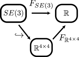
Figure 2: Commutative diagram highlighting how the natural embedding $\hookrightarrow:SE(3)\rightarrow\mathbb{R}^{4\times 4}$ can be used to restrict a general matrix function to $SE(3)$.

We briefly highlight how to represent scalar-valued functions $F_{SO(3)}:SO(3)\rightarrow\mathbb{R}$ and $F_{SE(3)}:SE(3)\rightarrow\mathbb{R}$. One approach is to define functions on manifolds by restricting a function defined on an embedding space $\mathbb{R}^{n\times n}$ Falorsi2020 . For Lie groups, it is immediately applicable whenever a matrix representation is available.

For example, on $SE(3)$ one restricts a function $F_{\mathbb{R}^{4\times 4}}:\mathbb{R}^{4\times 4}\rightarrow\mathbb{R}$ to arguments from $SE(3)\subset\mathbb{R}^{4\times 4}$, see Figure 2. The gradient of such functions are computed by an application of equation (3.4):

$$\text{d}_{H}F_{SE(3)}=\frac{\partial}{\partial q}F_{SE(3)}\big{(}H(I+\tilde{q})\big{)}_{q=0}\,.$$ (54)

The approach also holds for $SO(3)$, which can be embedded in $\mathbb{R}^{3\times 3}$, instead of $\mathbb{R}^{4\times 4}$.

5 Optimizing a rigid body control

The optimization procedure in Section 2 is applied to potential energy and damping injection based control of a fully actuated rigid body.

The core idea of potential energy shaping and damping injection is to combine advantages of energy-balancing passivity based control (EB-PBC) Ortega2000 and of control by interconnection Ortega2008 , which provide stability guarantees when interfacing with physical systems. Our article presents a class of controllers that generalizes the architecture presented by Rashad et al. Rashad2019 . We address common safety concerns about machine learning in control loops by optimizing a class of controllers that guarantees stability and a bounded energy by design.

5.1 Control of a rigid body

The trajectory of a rigid body in Euclidean 3-space is fully described by the curve $H^{0}_{b}:\mathbb{R}\rightarrow SE(3)$ that gives the relative position and orientation of a frame $\Psi_{b}$ attached to the rigid body with respect to an inertial frame $\Psi_{0}$ (see Remark 4.1). Following equation (39), the twist of the body with respect to $\Psi_{0}$, expressed in the body frame $\Psi_{b}$ is

$$T^{b,0}_{b}=\Lambda^{-1}(H^{b}_{0}\dot{H}^{0}_{b})\,.$$ (55)

Given the inertia tensor $\mathcal{I}\in\mathbb{R}^{6\times 6}$, $P^{b}=\mathcal{I}T^{b,0}_{b}\in\mathbb{R}^{6}$ represents the momentum in the body frame. The indices remain fixed in the subsequent treatment, and are suppressed to avoid cluttering (i.e., $H:=H^{0}_{b},\,T:=T^{b,0}_{b},\,P:=P^{b})$.

The dynamics of a rigid body follow from the Hamiltonian equations on matrix Lie groups ((100) and (101) in Appendix A.2) by setting $G=SE(3)$ and letting $\mathcal{H}(H,P)=\frac{1}{2}{P}^{\top}\mathcal{I}^{-1}P$. Including an external input wrench $W\in\mathbb{R}^{6}$, the dynamics read:

$$\dot{H} =H\Lambda(\mathcal{I}^{-1}P)\,,$$ (56)

$$\dot{P} =\text{ad}_{\mathcal{I}^{-1}P}^{\top}P+W\,.$$ (57)

In control by potential energy shaping and damping injection, this external wrench is constructed as a sum of a potential gradient term $W_{V}$ and a damping term $W_{D}$:

$$W=W_{V}+W_{D}\,.$$ (58)

In our approach the potential gradient term

$$W_{V}=-\text{d}_{H}V$$ (59)

is computed by an application of equation (54).

Nonlinear, configuration-dependent viscous damping takes the form

$$W_{D}=-B(H,P)P\,,$$ (60)

with $B(H,P)\mathcal{I}\in\mathbb{R}^{6\times 6}$ a symmetric and positive definite matrix.

Remark 5.1.

In this context, the control architecture of Rashad et al. Rashad2019 corresponds to the popular yet very particular choice of a constant $B(H,P)$ for the damping injection, while their potential $V(H)$ shows a quadratic dependence on translations and a nearly quadratic dependence on rotations. Their controller may be interpreted as a linear PD controller on $SE(3)$, where our work may be seen as a nonlinear PD controller on $SE(3)$.

5.2 Stability

We present here a general proof of stability for the class of controllers.

Theorem 5.1 (Stability).

Given the system (56), (57) together with the controller (58) given as

$$W(H,P)=-\text{d}_{H}V-B(H,P)P\,.$$ (61)

If $\forall H\in SE(3),P\in\mathbb{R}^{6}:B(H,P)\mathcal{I}>0$ and $V:SE(3)\rightarrow\mathbb{R}$ is lower-bounded, then $\lim_{t\rightarrow\infty}P(t)=0$ and any local minimum of $V$ is locally asymptotically stable.

Proof.

With $\text{E}_{\text{Pot}}=V(H)$ and $\text{E}_{\text{Kin}}=\frac{1}{2}{P}^{\top}\mathcal{I}^{-1}P$, take the system’s total energy $\text{E}=\text{E}_{\text{Pot}}+\text{E}_{\text{Kin}}$ as the Lyapunov function candidate. Then

$$\dot{\text{E}}_{\text{Pot}} =(\text{d}_{H}V)^{\top}T$$ (62)

$$\dot{\text{E}}_{\text{Kin}} =(\dot{P})^{\top}\mathcal{I}^{-1}P=(\dot{P})^{\top}T$$ (63)

$$=(\text{ad}^{\top}_{T}P-\text{d}_{H}V)^{\top}T-(P)^{\top}BT$$

$$=(-\text{d}_{H}V)^{\top}T-T^{\top}B\mathcal{I}T\,,$$

such that

$$\dot{\text{E}}=\dot{\text{E}}_{\text{Pot}}+\dot{\text{E}}_{\text{Kin}}=-T^{\top}B\mathcal{I}T\leq 0\,.$$ (64)

By LaSalle’s invariance principle, the system converges to the greatest invariant subset where $\dot{E}=0$. Since $B(H,P)>0$, the set with $\dot{E}=0$ is simply the set

$$S=\{(H,P)\,|\,P=0\}\,.$$ (65)

By inspection of the dynamics (57) the greatest invariant subset of $S$ is the set with $\text{d}_{H}V=0$, corresponding to the maxima and minima of $V$. Since $\dot{E}\leq 0$, the system cannot converge to maxima of $V$, leaving the minima of $V$ as limit sets and local minima of $V$ as asymptotically stable equilibria. ∎∎

5.3 Optimization by the adjoint method on SE(3)

In order to apply the adjoint method on Lie groups (Theorem 2.1), we re-define the dynamics (56) and (57) on the Lie group $G=SE(3)\times se^{*}(3)$. To this end, we choose to equip $G$ with the element-wise composition $(H_{1},P_{1})\circ(H_{2},P_{2})=(H_{1}H_{2},P_{1}+P_{2})$.

As a composition of matrix Lie groups $SE(3)$ and $(\mathbb{R}^{6},+)$, $G\subset GL(11,\mathbb{R})$ is defined as

$$G:=\{\begin{bmatrix}H&0&0\\ 0&I&P\\ 0&0&1\end{bmatrix}\,|\,H\in SE(3),P\in\mathbb{R}^{6}\}\,,$$ (66)

where matrix multiplication indeed corresponds to the element-wise composition in the abstract $G$. For details on the construction of $G$, the Lie algebra $\mathfrak{g}$, the choice of Lie algebra representation $\Lambda:\mathbb{R}^{12}\rightarrow\mathfrak{g}$, adjoint map and exponential map see Appendix B.5.2. The dynamics for $\Gamma(t)\in G$ read

$$\dot{\Gamma} =f_{\theta}(\Gamma)=\begin{bmatrix}\dot{H}(H,P)&0&0\\ 0&0&\dot{P}_{\theta}(H,P)\\ 0&0&0\end{bmatrix}\,,$$ (67)

where

$$\dot{H}(H,P) =H\Lambda(\mathcal{I}^{-1}P)\,,$$ (68)

$$\dot{P}_{\theta}(H,P) =\text{ad}_{\mathcal{I}^{-1}P}^{\top}P+W_{\theta}(H,P)\,.$$ (69)

Here, the control-wrench $W_{\theta}:SE(3)\times\mathbb{R}^{6}\rightarrow\mathbb{R}^{6}$ is parameterized by $\theta\in\mathbb{R}^{n_{\theta}}$.

Given a cost $C^{T}_{f_{\theta}}(\Gamma,\theta)$ of the type (10) and a distribution $\mathbb{P}$ of initial conditions $\Gamma_{0}$, define an optimization problem in the form of (11):

$$\min_{\theta}\,\mathbb{E}_{\Gamma_{0}\sim\mathbb{P}(\Gamma_{0})}[C(\Gamma_{0},\theta)]=\min_{\theta}J(\theta)\,.$$ (70)

As in Section 2.3, approximate $J(\theta)\approx\sum_{i=0}^{N}C^{T}_{f_{\theta}}(\Gamma_{i},\theta)$ and apply Theorem 2.1 to compute the parameter gradient of the $C^{T}_{f_{\theta}}(\Gamma_{i},\theta)$ by equation (15).

The dynamics of $\lambda_{\Gamma}$ follow from equation (17) as

$$\dot{\lambda}_{\Gamma}=-\text{d}_{\Gamma}\bigg{(}\lambda_{\Gamma}\big{(}\Lambda^{-1}(\tilde{f}_{\theta}(\Gamma)\big{)}+r(\Gamma,\theta)\bigg{)}+\text{ad}_{\tilde{f}_{\theta}}^{\top}\lambda_{\Gamma}\,,$$ (71)

$$\lambda_{\Gamma}(T)=\text{d}_{\Gamma}F\,,$$ (72)

where $\Lambda^{-1}(\tilde{f}_{\theta})$ is

$$\Lambda^{-1}(\tilde{f}_{\theta}) :=\Lambda^{-1}\big{(}\Gamma^{-1}f_{\theta}(\Gamma)\big{)}=\begin{pmatrix}\mathcal{I}^{-1}P\\ \dot{P}_{\theta}(H,P)\end{pmatrix}\,.$$ (73)

The gradient $\text{d}_{\Gamma}:C^{1}(G,\mathbb{R})\rightarrow\mathbb{R}^{12}$ is given by Equation (3.4). We split it into components $\text{d}_{H}:C^{1}(SE(3),\mathbb{R})\rightarrow\mathbb{R}^{6}$ and $\text{d}_{P}:C^{1}(\text{Vec}(6,\mathbb{R}),\mathbb{R})\rightarrow\mathbb{R}^{6}$ defined on the Lie groups $SE(3)$ and $(\mathbb{R}^{6},+)$, respectively.

Further, split $\lambda_{\Gamma}=(\lambda_{H},\lambda_{P})$ into components $\lambda_{H},\lambda_{P}\in\mathbb{R}^{6}$, and write out the control wrench $W_{\theta}(H,P)=-\text{d}_{H}V_{\theta}-B_{\theta}(H,P)P$. Then the equation for $\dot{\lambda}_{\Gamma}$ can be resolved to

$$\dot{\lambda} {}_{\Gamma}=$$ (74)

$$\begin{pmatrix}\text{d}_{H}\big{(}\lambda_{P}^{\top}(\text{d}_{H}V_{\theta}+B_{\theta}(H,P)P)-r(\Gamma,\theta)\big{)}-\text{ad}_{\mathcal{I}^{-1}P}^{\top}\lambda_{H}\\ \text{d}_{P}\big{(}\lambda_{P}^{\top}(B_{\theta}(H,P)P-\text{ad}_{\mathcal{I}^{-1}P}^{\top}P)-r(\Gamma,\theta)\big{)}-\mathcal{I}^{-1}\lambda_{H}\end{pmatrix}\,,$$

$$\Lambda {}_{H}(T)=\text{d}_{H}F\,,\;\Lambda_{P}(T)=\text{d}_{P}F\,.$$

Remark 5.2.

Note that the second derivative term $\text{d}_{H}\big{(}\lambda_{P}^{\top}(\text{d}_{H}V_{\theta})\big{)}$ in the dynamics (74) is well defined, since $\lambda_{P}^{\top}(\text{d}_{H}V_{\theta})\in C^{1}(SE(3),\mathbb{R})$.

Remark 5.3.

Rather than constructing the direct product group $SE(3)\times se^{*}(3)$, the semi-direct product group $SE(3)\ltimes se^{*}(3)$ could have been defined using the Coadjoint representation $Ad_{H}^{*}:se^{*}(3)\rightarrow se^{*}(3)$, leading to the group operation $(H_{1},P_{1})\bullet(H_{2},P_{2})=(H_{1}H_{2},P_{1}+Ad_{H_{1}}^{*}P_{2})$. Since an alternative choice of group action does not affect the optimum of the optimization, use of the semi-direct product group was not further investigated.

6 Simulations

We numerically solve the optimization problem (11) for the dynamics (67). We investigate various choices of final and running costs, distributions $\mathbb{P}$ and parameterizations of $V_{\theta}$, $B_{\theta}$.

6.1 Quadratic vs. general potential shaping

A controller with quadratic potential and linear damping injection (Section 6.1.2) is compared to a controller with NN-parameterized potential and damping injection (Section 6.1.3).

6.1.1 Choice of cost $C$ and distribution $\mathbb{P}$:

We determine a final cost $F$ and a running cost $r$ to stabilize a static target state with $H=H_{F},\,P=0$ over a horizon of $T=3$ seconds. The key properties of $F$ and $r$ are that both are differentiable and have their minimum in the target pose. Denote components of $H$ and $P$

$$H=\begin{bmatrix}R&p\\ 0&1\end{bmatrix}\,,\;P=\begin{pmatrix}P_{\omega}\\ P_{v}\end{pmatrix}\,,$$

where $R\in\mathbb{R}^{3\times 3}$, and $p,P_{\omega},P_{v}\in\mathbb{R}^{3}$. With weights $w_{1},\ldots,w_{9}\in\mathbb{R}_{+}$, we choose $F$ and $r$ as

$$F(\Gamma)= -w_{1}\text{Tr}(H_{F}^{-1}H)+w_{2}\|d\|_{2}^{2}$$ (75)

$$+w_{3}\|P_{\omega}\|^{2}+w_{4}\|P_{v}\|_{2}^{2}\,,$$

$$r(\Gamma)= -w_{5}\text{Tr}(H_{F}^{-1}H)+w_{6}\|d\|_{2}^{2}$$ (76)

$$+w_{7}\|P_{\omega}\|^{2}+w_{8}\|P_{v}\|_{2}^{2}+w_{9}\|W_{\theta}(H,P)\|^{2}\,.$$

Given scalars $\alpha,d,\theta_{p},d_{p}\in\mathbb{R}$ and vectors $\omega,v,\omega_{p},v_{p}\in\mathbb{R}^{3}$, and an average initial pose $H_{I}=H_{F}$, an initial condition $\Gamma_{0}$ is constructed as

$$\Gamma_{0}=\begin{pmatrix}H\\ P\end{pmatrix}$$ (77)

$$q=\begin{pmatrix}\alpha\omega/\|\omega\|_{2}\\ dv/\|v|_{2}\end{pmatrix}\,,$$ (78)

$$H=H_{I}\text{exp}(\tilde{q})\,,$$ (79)

$$P=\begin{pmatrix}\alpha_{p}\omega_{p}/\|\omega_{p}\|_{2}\\ d_{p}v_{p}/\|v_{p}|_{2}\end{pmatrix}\,.$$ (80)

The distribution $\mathbb{P}$ of $\Gamma_{0}$ is implemented by sampling

$$\alpha\sim\text{Uniform}[0,\pi]\,,\quad d\sim\text{Uniform}[0,1]\,,$$ (81)

$$\alpha_{p}\sim\text{Uniform}[0,0.03]\,,\quad d_{p}\sim\text{Uniform}[0,1]\,,$$ (82)

and sampling $\omega,v,\omega_{p},v_{p}\in\mathbb{R}^{3}$ from a normal distribution $\mathcal{N}(\mu,\sigma^{2})$ with standard deviation $\mu=(0,0,0)^{T}$ and variance $\sigma^{2}=I_{3\times 3}$.

6.1.2 Quadratic potential and linear damping injection:

The quadratic controller coincides with the controller presented by Rashad et al. Rashad2019 , in a setting of motion control. As such the quadratic potential $V_{Q,\theta}:SE(3)\rightarrow\mathbb{R}$ is given by

$$V_{Q,\theta}(\begin{bmatrix}R&p\\ 0&1\end{bmatrix})=\, \frac{1}{4}p^{\top}K_{\theta}p+\frac{1}{4}p^{\top}RK_{\theta}R^{\top}p$$ (83)

$$-\text{Tr}(G_{\theta}(R-I_{3}))\,,$$

and the constant damping injection is characterized by

$$B_{Q,\theta}(H,P)=B_{Q,\theta}\in\mathbb{R}^{6\times 6}\,.$$ (84)

Here the translational stiffness matrix $K_{\theta}\in\mathbb{R}^{3\times 3}$, the rotational co-stiffness matrix $G_{\theta}\in\mathbb{R}^{3\times 3}$ and the damping injection matrix $B_{Q,\theta}$ are chosen as

$$K_{\theta} =\begin{bmatrix}\exp(\theta_{1})&0&0\\ 0&\exp(\theta_{2})&0\\ 0&0&\exp(\theta_{3})\\ \end{bmatrix}$$ (85)

$$G_{\theta} =\begin{bmatrix}\exp(\theta_{4})&0&0\\ 0&\exp(\theta_{5})&0\\ 0&0&\exp(\theta_{6})\\ \end{bmatrix}$$ (86)

$$B_{Q,\theta} =\begin{bmatrix}\exp(\theta_{7})&0&0&0&0&0\\ 0&\exp(\theta_{8})&0&0&0&0\\ 0&0&\exp(\theta_{9})&0&0&0\\ 0&0&0&\exp(\theta_{10})&0&0\\ 0&0&0&0&\exp(\theta_{11})&0\\ 0&0&0&0&0&\exp(\theta_{12})\\ \end{bmatrix}$$ (87)

where the diagonal elements $\exp(\theta_{i})$ ensure that the matrices are positive definite. Note that the conditions of Theorem 5.1 are guaranteed: $V_{Q}$ is lower bounded, and for the diagonal, positive definite $B_{Q,\theta}$ also symmetry of $B_{Q,\theta}\mathcal{I}$ is guaranteed.

The control-law is then of the form

$$W_{Q,\theta}(H,P)=-\text{d}_{H}V_{Q,\theta}-B_{Q,\theta}P\,.$$ (88)

The parameters are optimized over $1200$ training epochs, using the ADAM optimizer with decay $\gamma=0.999$, a learning rate of $\eta=0.001$ for the initial $1000$ epochs and restarting training at a learning rate of $\eta=0.01$ for the final $200$ epochs. Additional parameters of the training are summarized in Appendix C.1, Table 1. The training progress is summarized in Figure 3, where Figure 3(a) shows a monotonous decrease of the cost function over the training epochs, while Figures 3(b) and 3(c) indicate a steady improvement of the final system states with respect to the target pose. The resulting controller’s performance is shown in Figure 4. Here Figures 4(a) and 4(b) show that the controlled rigid bodies approach the target configuration. Figure 4(c) shows that the controller uses the potential $V_{Q,\theta}$ to guide the rigid bodies towards the target pose, and that kinetic energy is quickly dissipated.

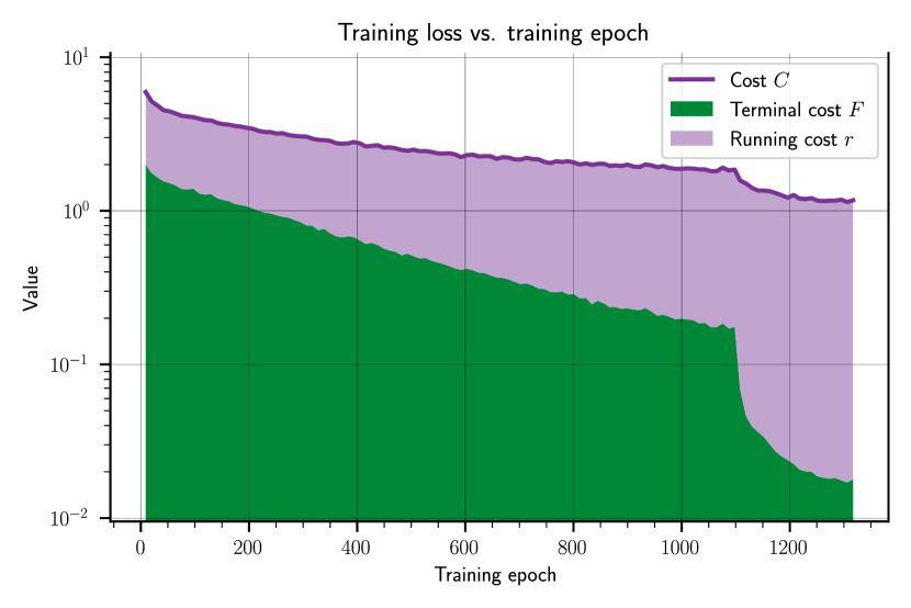
(a) Loss, terminal loss and integral loss.

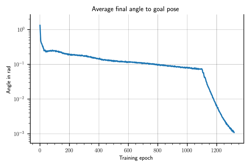
(b) Average final angle towards goal pose.

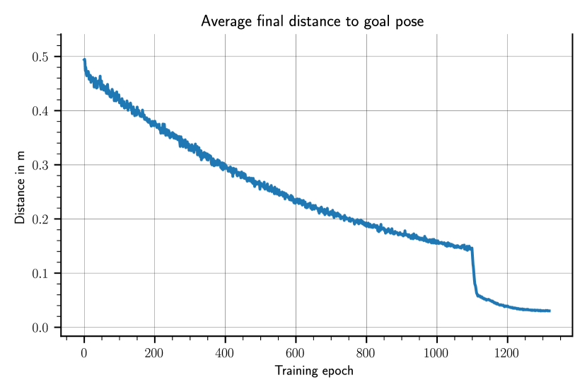
(c) Average final distance towards goal pose.

Figure 3: Visualization of the training progress of the quadratic controller characterized by $V_{Q,\theta}$ and $B_{Q,\theta}$. All figures show data averaged over 2048 sample trajectories at the given epoch, with initial conditions sampled from $\mathbb{P}(\Gamma_{0})$.

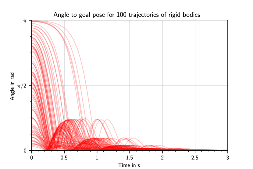
(a) Angle towards goal pose over 3 seconds.

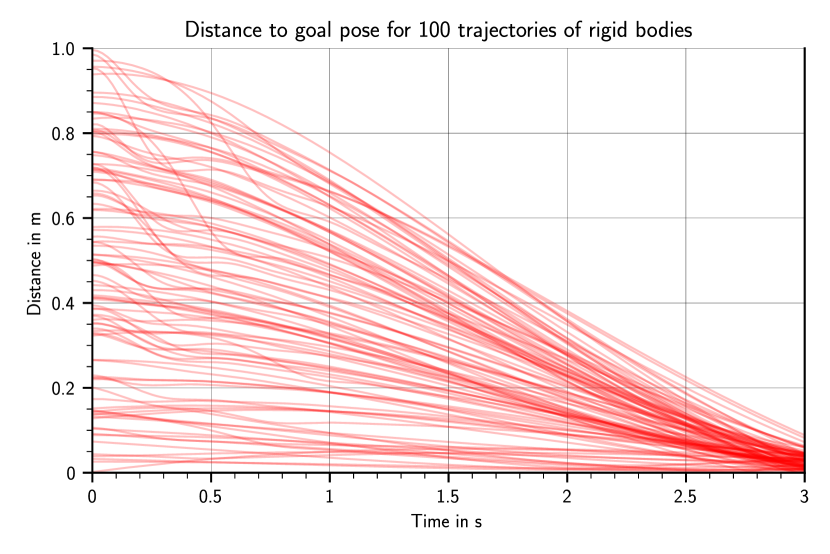
(b) Distance towards goal pose over 3 seconds.

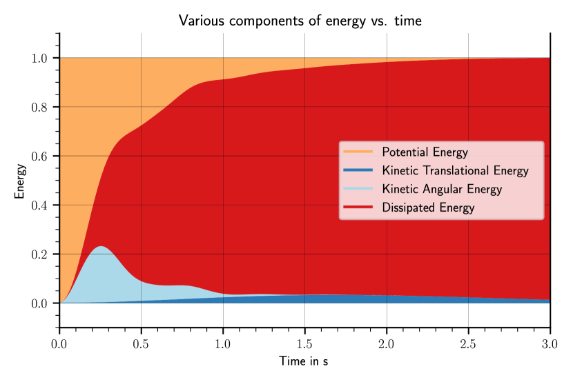
(c) Average proportions of system energy over 3 seconds.

Figure 4: Visualization of the performance of the quadratic controller characterized by $V_{Q,\theta}$ and $B_{Q,\theta}$, over 100 trajectories of rigid bodies with initial conditions sampled from $\mathbb{P}(\Gamma_{0})$.

6.1.3 Nonlinear potential and damping injection:

Here we showcase the optimization of a nonlinear potential $V_{N,\theta}:SE(3)\rightarrow\mathbb{R}$ and a nonlinear damping injections $B_{N,\theta}(H,P)\in\mathbb{R}^{6\times 6}$. Both functions are parameterized by neural nets with one hidden layer of 64 neurons, using softplus and tanh activation functions. $V_{N,\theta}$ has 12 inputs (the components of $R$ and $p$, this is a projection of $H$) and 1 output, while $B_{N,\theta}$ has 18 inputs (components of $R$, $p$ and $P$) and 6 outputs, which are then put through an element-wise exponential function and turned into a diagonal 6 by 6 matrix to guarantee positive-definiteness of $B_{N,\theta}(H,P)\mathcal{I}$.

The control law is of the form

$$W_{N,\theta}(H,P)=-\text{d}_{H}V_{N,\theta}-B_{N,\theta}(H,P)P\,.$$ (89)

The parameters are optimized over $1000$ training epochs, using the ADAM optimizer with decay $\gamma=0.999$, and a learning rate of $\eta=0.001$. Additional parameters of the training are summarized in Appendix C.1, Table 2.

The training progress is summarized in Figure 5. It can be seen that the final loss of the nonlinear controller in Figure 5(a) is equivalent to that of the quadratic controller Figure 3(a). In particular, the performance of a quadratic and a nonlinear controller for this scenario are close: the final angle and distance in Figures 5(b) and 5(c) are comparable to those of Figures 3(b) and 3(c), respectively. The resulting controller’s performance is shown in Figure 6. Here the qualitative behavior shown in Figures 6(a), 6(b) and 6(c) resembles that of the quadratic case in Figures 4(a), 4(b) and 4(c), respectively.

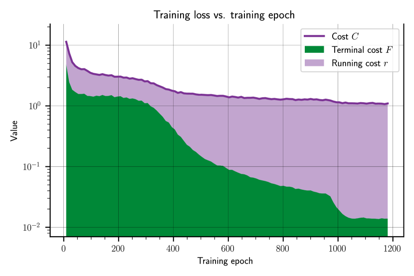
(a) Loss, terminal loss and integral loss.

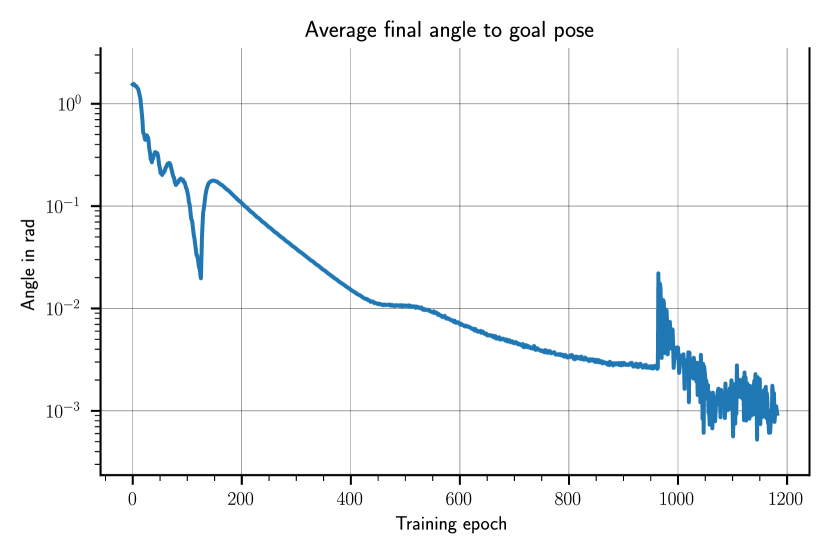
(b) Average final angle towards goal pose.

(c) Average final distance towards goal pose.

Figure 5: Visualization of the training progress of the nonlinear controller characterized by $V_{N,\theta}$ and $B_{N,\theta}$. All figures show data averaged over 2048 sample trajectories at the given epoch, with initial conditions sampled from $\mathbb{P}$.

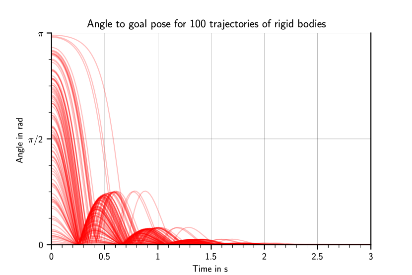
(a) Angle towards goal pose over 3 seconds.

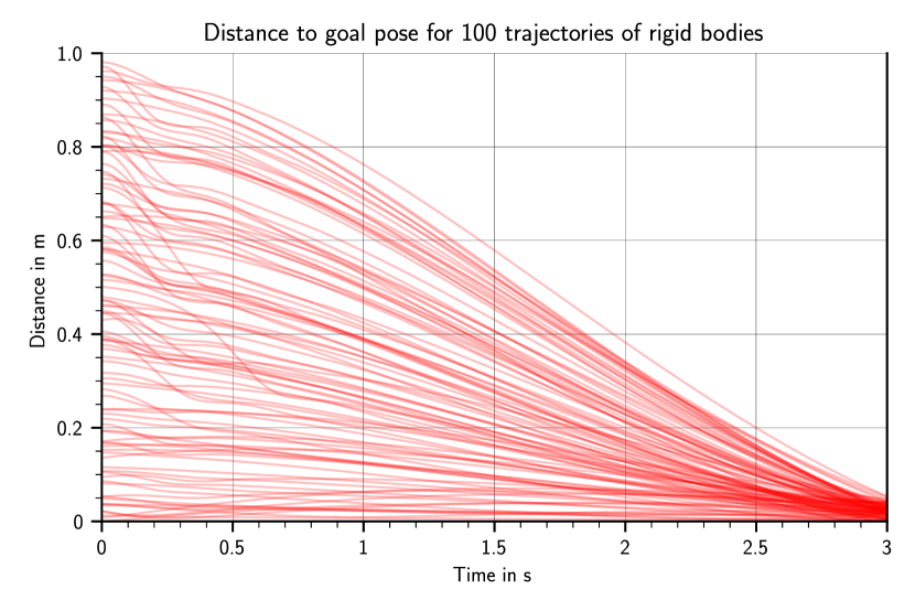
(b) Distance towards goal pose over 3 seconds.

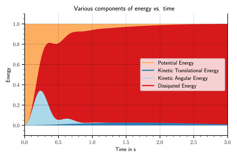
(c) Average proportions of system energy over 3 seconds.

Figure 6: Visualization of the performance of the nonlinear controller characterized by $V_{N,\theta}$ and $B_{N,\theta}$, over 100 trajectories of rigid bodies with initial conditions sampled from $\mathbb{P}(\Gamma_{0})$.

6.2 General potential shaping with gravity

We optimize an NN-parameterized potential and damping injection in a system with gravity in Section 6.2.2, and show the effect of an adapted target configuration in Section 6.2.3.

6.2.1 Adapted running cost $r$:

In the presence of a gravitational potential $V_{g}:SE(3)\rightarrow\mathbb{R}$ the momentum dynamics of a controlled rigid body (69) pick up an additional term $-\text{d}_{H}V_{g}$:

$$\dot{P}_{\theta}(H,P)=\text{ad}_{\mathcal{I}^{-1}P}^{\top}P+W_{\theta}(H,P)-\text{d}_{H}V_{g}\,.$$ (90)

The gravitational potential is unbounded: it can therefore not be globally compensated for by a bounded potential $V_{N,\theta}$. To circumvent this issue, we separately implement gravity compensation $W_{g}(H)=\text{d}_{H}V_{g}$ by choosing the total control wrench as

$$W_{\theta}(H,P)=W_{g}(H)+W_{N,\theta}(H,P)\,.$$ (91)

such that the momentum dynamics again read

$$\dot{P}_{\theta}(H,P)=\text{ad}_{\mathcal{I}^{-1}P}^{\top}P+W_{N,\theta}(H,P)\,.$$ (92)

To take gravity into account in the optimization, the only required adaptation is to use the adapted $W_{\theta}(H,P)$ in the running-cost (76).

Minimizing the term $\|W_{\theta}(H,P)\|$ indirectly minimizes the required gravity compensation by reducing the total wrench exerted on the plant. Indeed, when $\|W_{\theta}\|=0$ the dynamics are

$$\dot{P}_{\theta}(H,P)=\text{ad}_{\mathcal{I}^{-1}P}^{\top}P-\text{d}_{H}V_{g}\,.$$ (93)

Thus, for $\|W_{\theta}\|=0$ the learned control-action $W_{N,\theta}(H,P)$ cancels the gravity compensation, such that the external gravitational potential is utilized to exert a force on the rigid body.

6.2.2 Nonlinear potential and damping injection:

Here, we apply the ADAM optimizer with learning rate $\eta=0.001$ and decay $\gamma=0.999$ to optimize the nonlinear potential $V_{N,\theta}$ and damping $B_{N,\theta}$ for an adapted running cost. Additional parameters of the training are summarized in Appendix C.1, Table 3. The training progress is summarized in Figure 7, and the resulting controller’s performance is shown in Figure 8. Notably, the results do not differ strongly from Figures 5 and 4.

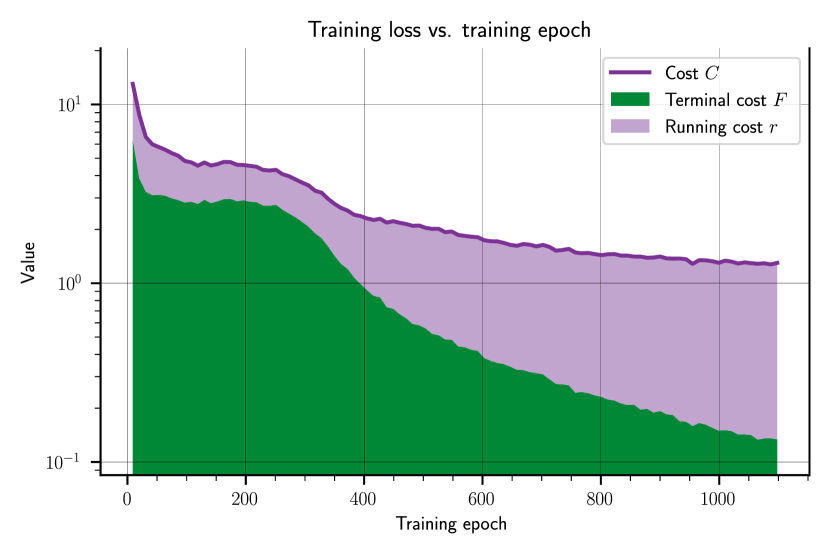
(a) Loss, terminal loss and integral loss.

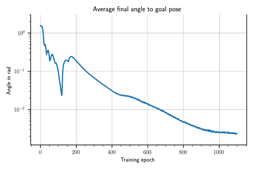
(b) Average final angle towards goal pose.

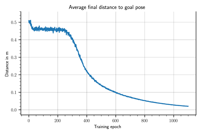
(c) Average final distance towards goal pose.

Figure 7: Visualization of the training progress of the nonlinear controller characterized by $V_{N,\theta}$ and $B_{N,\theta}$, in the presence of gravity. All figures show data averaged over 2048 sample trajectories at the given epoch, with initial conditions sampled from $\mathbb{P}(\Gamma_{0})$.

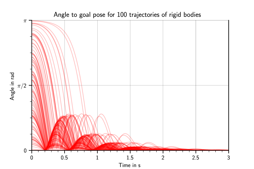
(a) Angle towards goal pose over 3 seconds.

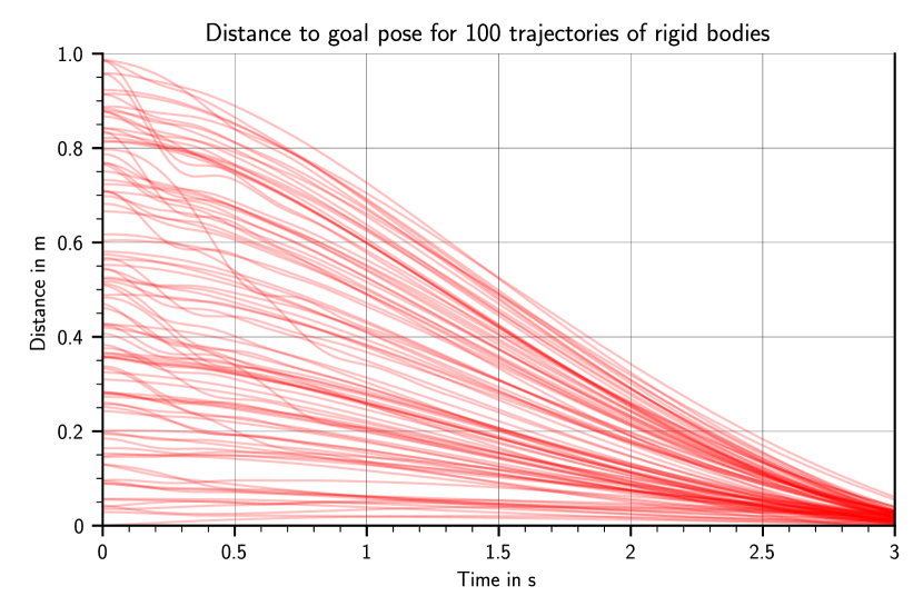
(b) Distance towards goal pose over 3 seconds.

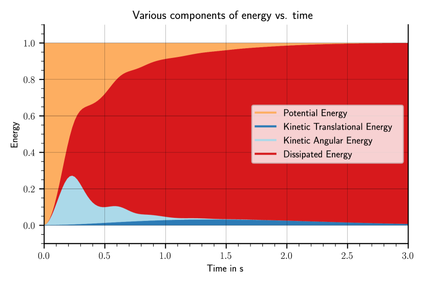
(c) Average proportions of system energy over 3 seconds.

Figure 8: Visualization of the performance of the nonlinear controller characterized by $V_{N,\theta}$ and $B_{N,\theta}$, in the presence of gravity. The results show 100 trajectories of rigid bodies with initial conditions sampled from $\mathbb{P}(\Gamma_{0})$.

6.2.3 Asymmetric initial distribution:

To better highlight the influence of the adapted running cost, and how the optimization in the presence of gravity differs from an optimization in the absence of gravity, an initial distribution asymmetric about the goal pose $H_{F}$ (77) is introduced by choosing

$$H_{F}=\begin{bmatrix}I&d_{F}\\ 0&1\end{bmatrix}$$

with $d_{F}=(0,0,-1)^{T}$.

The parameters of this training coincide with those of the symmetric scenario, and are likewise summarized in Appendix C.1, Table 3. The training progress is summarized in Figure 9, and the resulting controller’s performance is shown in Figure 10.

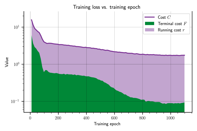
(a) Loss, terminal loss and integral loss.

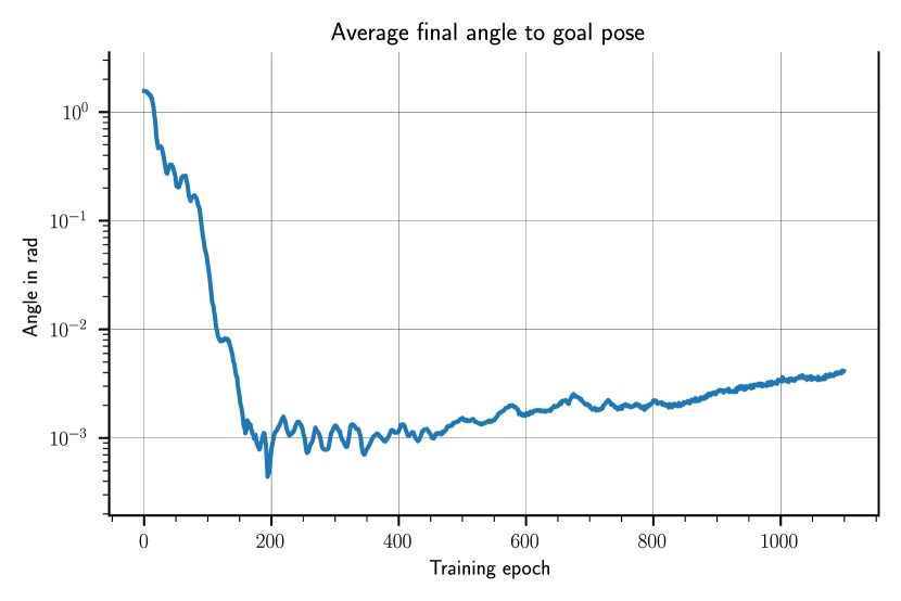
(b) Average final angle towards goal pose.

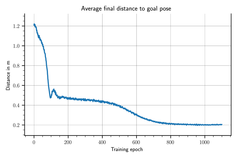
(c) Average final distance towards goal pose.

Figure 9: Visualization of the training progress of the nonlinear controller characterized by $V_{N,\theta}$ and $B_{N,\theta}$, in the presence of gravity and with an initial distribution whose mean is above the target position. All figures show data averaged over 2048 sample trajectories at the given epoch, with initial conditions sampled from $\mathbb{P}(\Gamma_{0})$.

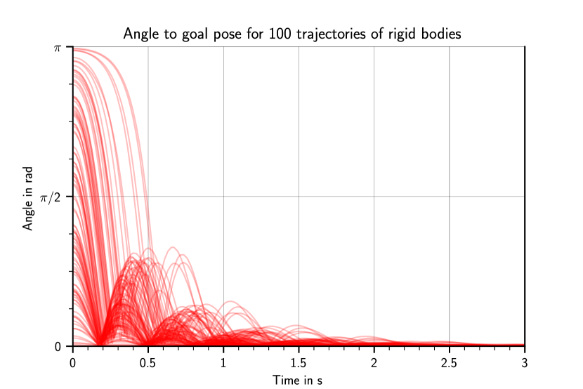
(a) Angle towards goal pose over 3 seconds.

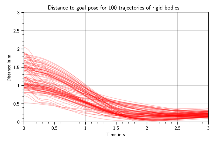
(b) Distance towards goal pose over 3 seconds.

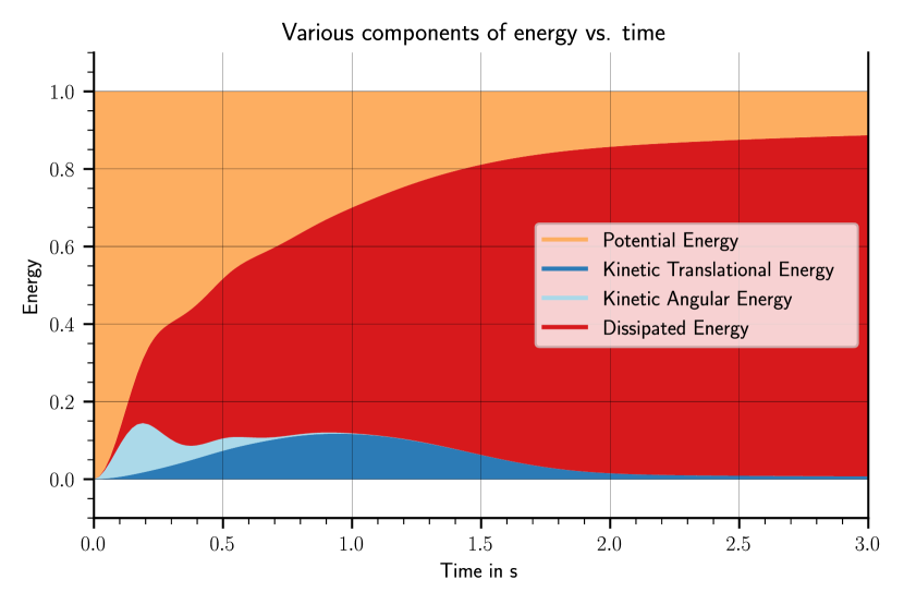
(c) Average proportions of system energy over 3 seconds.

Figure 10: Visualization of the performance of the nonlinear controller characterized by $V_{N,\theta}$ and $B_{N,\theta}$, in the presence of gravity and with an initial distribution whose mean is above the target position. The results show 100 trajectories of rigid bodies with initial conditions sampled from $\mathbb{P}(\Gamma_{0})$.

7 Discussion

7.1 Neural ODEs on Lie groups

The proposed formulation of neural ODEs on Lie groups immediately applies to arbitrary matrix Lie groups, where parameterized maps can be learned with a global validity. The optimization of Neural ODEs on Lie groups by the gradient descent via the generalized adjoint method is a scalable approach. The key aspects that contribute to this scalability are: First, the generalized adjoint method on Lie groups preserves the memory efficiency of the generalized adjoint method used for neural ODEs on $\mathbb{R}^{k}$. Second, the formulation of the adjoint dynamics at the algebra level achieves a dimensionality reduction with respect to extrinsic formulations Duong2021_nODE_SE3 Falorsi2020 . Finally, this formulation at the algebra level also alleviates the need for chart-switches of the adjoint state, and it allows for the use of the compact expression (3.4) of the gradient, bypassing the need for gradient computations in local charts.

The work can be generalized further: Theorem 2.1 assumes the cost to be of the form (10), while the derivation in Appendix A.4 in principle allows for a more general choice of cost that may be of interest in e.g. learning of periodic trajectories Wotte2023 . The accompanying code is currently written specifically for the Lie group $SE(3)\times\mathbb{R}^{6}$, and future work will produce code that is applicable to other matrix Lie groups as well.

7.2 Optimal Potential Shaping

The optimization of an NN-parameterized potential and damping injection was successful and confirms the scalability of the adjoint method on Lie groups. The optimization was also successful when including gravity in a nonlinear running cost. Stability was guaranteed by design, by implementing the requirements of Theorem 5.1 on the level of architecture and activation functions. As a further advantage the resulting controller is global on $SE(3)$, as opposed to only being applicable in a limited chart-region.

Regarding limitations of the approach, the numerical stability of the adjoint method on $SE(3)$ was observed to strongly depend on the smoothness of the running cost, which suggests added value in considering different Lie group integrators that accommodate this lack of smoothness. Lastly, while the structure of the presented controller is highly interpretable and the various components of the energy are readily visualized, the space of possible initial conditions and trajectories remains large, and the high dimensional state-space obscures low-level properties and a deep understanding of the eventual controller, beyond safety guarantees and numerical verification of stability.

Alternative choices for the final and running costs, as well as the weights in these costs are worth investigating. The design space of possible controllers is also large and other control architectures may be advantageous. In future work the controller will be applied to a real drone, and other cost functions and control structures will be investigated.

8 Conclusion

Lie groups are ubiquitous in engineering, and so are dynamic systems on Lie groups. We proposed a method for dynamics optimization that works on arbitrary, finite dimensional Lie groups and for a large class of cost functions. The resulting method is highly scalable, and more compact than alternative manifold formulations. The key steps in the formulation related to using canonical Lie group structure to create a compact gradient descent algorithm: we phrased the generalized adjoint method at the Lie algebra level, we utilize a compact expression for the gradient as an element of the dual to the Lie algebra, and we use a generic Lie group integrator for dynamics integration. The method was successfully applied to optimize a controller for a rigid body that is globally valid on the Lie group SE(3). A key aspect of choosing the class of controllers was stability by design, which guided the architecture of the neural nets that parameterize the potential energy shaping and damping injection controller.

The authors declare that they have no conflicts of interest.

This research was supported by the PortWings project funded by the European Research Council [Grant Agreement No. 787675].

Notes

1. 1 A more general definition of a matrix lie group $G$ allows for complex matrix Lie groups $G\subset GL(m,\mathbb{C})$ or quaternionic matrix Lie groups $G\subset GL(m,\mathbb{H})$. The results in our article immediately extend to such scenarios: a choice of basis for the Lie algebras $gl(m,\mathbb{C}),\,gl(m,\mathbb{H})$ leads to $\Lambda:\mathbb{R}^{n}\rightarrow\mathfrak{g}$ in Equation (3), such that relevant quantities like the adjoint map in (6), the adjoint state and its dynamics in Theorem 2.1 may again be expressed as real valued vectors and matrices.
2. 2 When directly working with matrix Lie groups (e.g, sola2021micro ) $\Lambda$ and $\Lambda^{-1}$ are often denoted as the so-called “hat” $\wedge:\mathbb{R}^{n}\rightarrow\mathbb{R}^{m\times m}$ and “vee” $\vee:\mathbb{R}^{m\times m}\rightarrow\mathbb{R}^{n}$ operators, respectively.
3. 3 The left-translation of a map $f:G\rightarrow\mathcal{M}$ is defined as $(L_{g}f):=f\circ L_{g^{-1}}$.
4. 4 Symmetry and positive definiteness of $B(H,P)$ are not well defined because it is a $(1,1)$ tensor: to be technically precise one must impose that the $(0,2)$ tensor $B(H,P)\mathcal{I}$ is symmetric and positive definite. This imposes that the rate of energy lost to damping $T^{\top}B\mathcal{I}T\geq 0$.

Appendix A The generalized adjoint method on Lie groups

In this Appendix the generalized adjoint method on matrix Lie groups (Theorem 2.1) is derived in four steps.

A.1 Notation

Given functions $\Phi_{1}\in C^{k}(\mathcal{M},\mathcal{N})$, $\Phi_{2}\in C^{k}(\mathcal{N},\mathcal{P})$, their composition is denoted $\Phi_{2}\circ\Phi_{1}\in C^{k}(\mathcal{M},\mathcal{P})$. $\Omega^{k}(\mathcal{M})$ denotes the set of $k$-forms over $\mathcal{M}$. The exterior derivative is denoted as $\text{d}:\Omega^{k}(\mathcal{M})\rightarrow\Omega^{k+1}(\mathcal{M})$, and the wedge product as $\wedge:\Omega^{q}(\mathcal{M})\times\Omega^{p}(\mathcal{M})\rightarrow\Omega^{q+p}(\mathcal{M})$. Given a product manifold $\mathcal{M}\times\mathcal{N}$, a function $V\in C^{1}(\mathcal{M}\times\mathcal{N},\mathbb{R})$, with $x\in\mathcal{M}$, $y\in\mathcal{N}$, denote by $\big{(}\text{d}_{x}V\big{)}(y)\in T^{*}_{x}\mathcal{M}$ the partial gradient at $x\in\mathcal{M}$. Given a vector field $f\in\Gamma(T\mathcal{M})$ and a $k$-form $\omega\in\Omega^{k}(\mathcal{M})$ denote by $\i_{f}:\Omega^{k}(\mathcal{M})\rightarrow\Omega^{k-1}(\mathcal{M})$ the insertion operator $\i_{f}(\omega):=\omega(f)$. Further denote by $\mathcal{L}_{f}:\Omega^{k}(\mathcal{M})\rightarrow\Omega^{k}(\mathcal{M})$ the Lie derivative with respect to $f$.

A.2 Hamiltonian systems on Lie groups

We briefly review Hamiltonian systems on manifolds, on Lie groups and on matrix Lie groups. For a detailed introduction to Hamiltonian systems see e.g., Abrahams and Ratiu FoundationsOfMechanics .

Define a symplectic manifold as $(\mathcal{M},\omega)$, with $\mathcal{M}$ a manifold and $\omega\in\Omega^{2}(\mathcal{M})$ the symplectic form. For Hamiltonian dynamics on manifolds, we are interested in the case where $\mathcal{M}=T^{*}\mathcal{Q}$ is the cotangent bundle of some manifold $\mathcal{Q}$. Specializing to Lie groups, we investigate the case where $\mathcal{Q}=G$ for some Lie group $G$.

Given coordinate maps $q^{i}:\mathcal{Q}\rightarrow\mathbb{R}$ on $\mathcal{Q}$ and induced coordinates $p_{i}$ in the basis $\text{d}q^{i}$ on $T_{q}^{*}\mathcal{Q}$, the symplectic form is canonically defined as $\omega=\text{d}\theta=\text{d}p_{i}\wedge\text{d}q^{i}$, with $\theta=p_{i}dq^{i}$ the coordinate independent tautological one-form. Then a Hamiltonian $H\in C^{1}(T^{*}\mathcal{Q},\mathbb{R})$ implicitly defines a unique vector field $X_{H}\in\Gamma(T^{*}\mathcal{Q})$ by demanding that

$$\text{d}H(Y)=\omega(X_{H},Y)$$ (94)

holds for any $Y\in\Gamma(T^{*}\mathcal{Q})$. In coordinates induced by $q^{i},p_{i}$, the corresponding vector field $X_{H}$ has the components

$$\dot{q}^{i} =\frac{\partial H}{\partial p_{i}}\,,$$ (95)

$$\dot{p}_{i} =-\frac{\partial H}{\partial q^{i}}\,.$$ (96)

On a Lie group $G$ a different formulation is possible: the group structure allows the identification $T^{*}G\equiv G\times\mathfrak{g}^{*}$, where $\mathfrak{g}^{*}=T^{*}_{e}G$ is the dual of the Lie algebra $\mathfrak{g}$. In the left identification, the left-translation map $L_{g}:G\rightarrow G$ associates any cotangent space $T^{*}_{g}G$ with $\mathfrak{g}^{*}$ by the pullback ${L_{g}}^{*}:T_{g}^{*}G\rightarrow\mathfrak{g}^{*}$. Using this identification, the Hamiltonian $\mathcal{H}:G\times\mathfrak{g}^{*}\rightarrow\mathbb{R}$ is defined in terms of $H:T^{*}G\rightarrow\mathfrak{g}$ as

$$\mathcal{H}(g,\bar{P})=H\big{(}g,(L_{g^{-1}}^{*}\bar{P})\big{)}\,.$$ (97)

Then the Hamiltonian vector-field as a section in $\Gamma(TG\times T\mathfrak{g}^{*})$ is:

$$\dot{g} ={L_{g}}_{*}(\text{d}_{\bar{P}}\mathcal{H})\,,$$ (98)

$$\dot{\bar{P}} =-\bar{\text{d}}_{g}\mathcal{H}+\text{ad}_{\text{d}_{\bar{P}}\mathcal{H}}^{*}\bar{P}\,,$$ (99)

where $\text{d}_{\bar{P}}\mathcal{H}\in T^{*}_{\bar{P}}\mathfrak{g}^{*}\cong\mathfrak{g}^{*}$, $\bar{\text{d}}_{g}\mathcal{H}\in\mathfrak{g}^{*}$ as in Equation (28), $\text{ad}^{*}:\mathfrak{g}\times\mathfrak{g}^{*}\rightarrow\mathfrak{g}^{*}$ is the dual of the adjoint map ad, defined by $(\text{ad}^{*}_{\tilde{A}}\bar{P})(\tilde{B})=\bar{P}(\text{ad}_{\tilde{A}}\tilde{B})$.

For a matrix Lie group the equations (98) and (99) read, in terms of component matrices:

$$\dot{g} =g\Lambda(\frac{\partial\mathcal{H}}{\partial P})\,,$$ (100)

$$\dot{P} =-\text{d}_{g}\mathcal{H}+\text{ad}_{\frac{\partial\mathcal{H}}{\partial P}}^{\top}P\,.$$ (101)

Here $P\in\mathbb{R}^{n}$ and $\frac{\partial}{\partial P}$ is the usual partial derivative, $\text{d}_{g}\mathcal{H}\in\mathbb{R}^{n}$ is interpreted as in (3.4) and $\Lambda:\mathbb{R}^{n}\rightarrow\mathfrak{g}$ as in (3).

A.3 The adjoint sensitivity

Given are a manifold $\mathcal{M}$, a Lipschitz vector field $f\in\Gamma(T\mathcal{M})$, the associated flow $\Psi_{f}^{t}:\mathcal{M}\rightarrow\mathcal{M}$ and a differentiable scalar-valued function $C:\mathcal{M}\rightarrow\mathbb{R}$. A solution $x(t)\in\mathcal{M}$ of the dynamics $f$ is given by

$$x(t):=\Psi_{f}^{t}(x_{0})\,,\;x_{0}\in\mathcal{M}\,.$$ (102)

We are interested in computing the gradient

$$\text{d}(C\circ\Psi_{f}^{T})(x_{0})=(\Psi_{f}^{T})^{*}\text{d}C\big{(}x(T)\big{)}\,,$$ (103)

whose expression is given by Theorem A.1 Falorsi2020 ; BulloLewis2005_Supplementary . To the best of the authors’ knowledge, the presented derivation is a contribution with respect to the existing literature and is an alternative to the one presented in BulloLewis2005_Supplementary .

Theorem A.1 (Adjoint sensitivity on manifolds).

The gradient of a function $C\circ\Psi_{f}^{T}$ is

$$\text{d}(C\circ\Psi_{f}^{T})=\lambda(0)\,,$$ (104)

where $\lambda(t)\in T^{*}_{x(t)}\mathcal{M}$ is the adjoint state. In a local chart $(U,X)$ of $\mathcal{M}$ with induced coordinates on $TU$ and $T^{*}U$, $x(t)$ and $\lambda(t)$ satisfy the dynamics

$$\dot{x}^{j} =f^{j}(x)\,,\;x(0)=x_{0}\,,$$ (105)

$$\dot{\lambda}_{i} =-\lambda_{j}\frac{\partial}{\partial x^{i}}f^{j}(x)\,,\;\lambda(T)=\text{d}C\big{(}x(T)\big{)}\,.$$ (106)

Proof.

Define the adjoint state $\lambda(t)\in T^{*}_{x(t)}\mathcal{M}$ as

$$\lambda(t) :=(\Psi_{f}^{T-t})^{*}\lambda_{T}\,,\;\lambda_{T}\in T_{x(T)}^{*}\mathcal{M}\,.$$ (107)

Let $\lambda_{T}=\text{d}C\big{(}x(T)\big{)}$, then Equation (104) is recovered:

$$\lambda(0)=(\Psi_{f}^{T})^{*}\lambda_{T}=(\Psi_{f}^{T})^{*}\text{d}C\big{(}x(T)\big{)}=(\text{d}C\circ\Psi^{T}_{f})(x_{0})\,,$$ (108)

where the final step uses Equation (103).

A derivation of the dynamics governing $\lambda(t)$ constitutes the remainder of this proof. To this end, note that the Lie derivative of $\lambda(t)$ is

$$\mathcal{L}_{f}\lambda(t) =\frac{d}{ds}\big{(}(\Phi^{s}_{f})^{*}\lambda(t+s)\big{)}_{s=0}$$ (109)

$$=\frac{d}{ds}\big{(}(\Phi^{s}_{f})^{*}(\Psi_{f}^{T-t-s})^{*}\lambda_{T}\big{)}_{s=0}$$

$$=\frac{d}{ds}\big{(}(\Psi_{f}^{T-t})^{*}\lambda_{T}\big{)}_{s=0}=0\,.$$

Instead of a curve $\lambda(t)$, consider a 1-form $\lambda\in\Omega^{1}(\mathcal{M})$ (denoted as $\lambda$ by an abuse of notation) that satisfies $\mathcal{L}_{f}\lambda=0$. This allows to apply Cartan’s formula, which we express in a local chart:

$$\mathcal{L}_{f}\lambda=\; \text{d}(\i_{f}\lambda)+\i_{f}\text{d}\lambda$$ (110)

$$= \frac{\partial}{\partial x^{i}}(\lambda_{j}f^{j})\text{d}x^{i}+(\frac{\partial}{\partial x^{k}}\lambda_{i})(\text{d}x^{k}\wedge\text{d}x^{i})(f^{j}\frac{\partial}{\partial x^{j}})$$

$$=\, \frac{\partial}{\partial x^{i}}(\lambda_{j}f^{j})\text{d}x^{i}+(\frac{\partial}{\partial x^{k}}\lambda_{i})f^{k}\text{d}x^{i}-(\frac{\partial}{\partial x^{k}}\lambda_{i})f^{i}\text{d}x^{k}$$

$$=\, \lambda_{j}\frac{\partial}{\partial x^{i}}f^{j}\text{d}x^{i}+(\frac{\partial}{\partial x^{k}}\lambda_{i})f^{k}\text{d}x^{i}=0\,.$$

In terms of components, one obtains the partial differential equation

$$\lambda_{j}\frac{\partial}{\partial x^{i}}f^{j}+f^{k}\frac{\partial}{\partial x^{k}}\lambda_{i}=0\,.$$ (111)

Impose that $\lambda(t)=\lambda\big{(}\Psi^{t}_{f}(x_{0})\big{)}$, then

$$\dot{\lambda}_{i}=f^{k}\frac{\partial}{\partial x^{k}}\lambda_{i}\,.$$ (112)

Combining Equations (111) and (112) leads to Equation (106):

$$\dot{\lambda}_{i}=-\lambda_{j}\frac{\partial}{\partial x^{i}}f^{j}\,.$$ (113)

∎∎

Theorem A.1 can be recast into a Hamiltonian form:

Lemma A.1 (Hamiltonian form of adjoint sensitivity).

Define the so-called control Hamiltonian

$$H_{c}:T^{*}\mathcal{M}\rightarrow\mathbb{R}\,;\;H_{c}(x,\lambda)=\lambda\big{(}f(x)\big{)}\,.$$ (114)

Then Hamilton’s equations (95) and (96) agree with the equations for the adjoint sensitivity (105) and (106), respectively:

$$\dot{x}^{j} =\frac{\partial H_{c}}{\partial\lambda_{j}}=f^{j}\,,$$ (115)

$$\dot{\lambda}_{i} =-\frac{\partial H_{c}}{\partial x^{i}}=-\lambda_{j}\frac{\partial}{\partial x^{i}}f^{j}\,.$$ (116)

Remark A.1.

The vector field $f^{\uparrow}\in\Gamma(TT^{*}\mathcal{M})$ defined by equations (115) and (116) is called the co-tangent lift of $f$.

A.4 Neural ODEs on Manifolds

We phrase the optimal control problem on a manifold $\mathcal{M}$. Let $\theta\in\mathcal{P}$ denote a parameter, and define the parameterized, dynamic system

$$f:\mathcal{P}\rightarrow\Gamma(T\mathcal{M})\,;\;f_{\theta}:=f(\theta)\in\Gamma(T\mathcal{M})\,.$$ (117)

For time-dependent dynamics, consider instead dynamics on the space-time manifold $\mathcal{M}\times\mathbb{R}$, with $f_{\theta}+\frac{\partial}{\partial t}\in\Gamma\big{(}T(\mathcal{M}\times\mathbb{R})\big{)}$. With the flow $\Psi_{f_{\theta}}^{t}:\mathcal{M}\rightarrow\mathcal{M}$, define the cost $C^{T}_{f}:\mathcal{M}\rightarrow\mathbb{R}$ as

$$C^{T}_{f_{\theta}}(x_{0},\theta)=F\big{(}\Psi^{T}_{f_{\theta}}(x_{0}),\theta\big{)}+\int_{0}^{T}r\big{(}\Psi^{s}_{f_{\theta}}(x_{0}),\theta,s\big{)}\text{d}s\,.$$ (118)

The parameter gradient $\text{d}_{\theta}C^{T}_{f_{\theta}}(x_{0},\theta)\in T^{*}_{\theta}\mathcal{P}$ is then computed by Theorem A.2:

Theorem A.2 (Generalized Adjoint Method on Manifolds).

Given the dynamics (117) and the cost (118), the parameter gradient $\text{d}_{\theta}C^{T}_{f_{\theta}}(x_{0},\theta)\in T^{*}_{\theta}\mathcal{P}$ is computed by

$$\text{d}_{\theta}C^{T}_{f_{\theta}}(x_{0},\theta)=\text{d}_{\theta}F+\int_{0}^{T}\text{d}_{\theta}\big{(}\lambda(f_{\theta})+r\big{)}\text{d}t\,.$$ (119)

where the state $x(t)\in\mathcal{M}$ and adjoint state $\lambda(t)\in T^{*}_{x(t)}\mathcal{M}$ satisfy

$$\dot{x}^{j} =f^{j}\,,\;x(0)=x_{0}\,,$$ (120)

$$\dot{\lambda}_{i} =-\lambda_{j}\frac{\partial}{\partial x^{i}}f^{j}-\frac{\partial r}{\partial x^{i}}\,,\;\lambda(T)=\text{d}C\big{(}x(T)\big{)}\,.$$ (121)

Proof.

Define the augmented state space as $\mathcal{M}^{\prime}=\mathcal{M}\times\mathcal{P}\times\mathbb{R}\times[0,T]$ with state $x^{\prime}:=(x,\theta,L,t)\in\mathcal{M}^{\prime}$. In addition, define the augmented dynamics $f_{\text{aug}}\in\Gamma(T\mathcal{M}^{\prime})$ as

$$f_{\text{aug}}(x^{\prime})=\begin{pmatrix}f_{\theta}(x,t)\\ 0\\ r(x,\theta,t)\\ 1\end{pmatrix}\,,\;x^{\prime}(0)=x^{\prime}_{0}:=\begin{pmatrix}x_{0}\\ \theta\\ 0\\ 0\end{pmatrix}\,.$$ (122)

Next, define the augmented cost $C_{\text{aug}}:\mathcal{M}^{\prime}\rightarrow\mathbb{R}$:

$$C_{\text{aug}}(x^{\prime})=F(x)+L\,.$$ (123)

Then Equation (118) can be rewritten as

$$C^{T}_{f_{\theta}}(x^{\prime}_{0})=(C_{\text{aug}}\circ\Psi_{f_{\text{aug}}}^{T})(x^{\prime}_{0})\,,$$ (124)

which is of the required form to apply Theorem A.1. By Theorem A.1, the gradient $\text{d}\big{(}C_{\text{aug}}\circ\Psi_{f_{\text{aug}}}^{T}\big{)}$ is given by

$$\text{d}(C_{\text{aug}}\circ\Psi_{f_{\text{aug}}}^{T})(x^{\prime}_{0})=\lambda(0)\,,$$ (125)

where $\lambda(t)$ satisfies

$$\dot{\lambda}_{i}=-\lambda_{j}\frac{\partial}{\partial x^{\prime}_{i}}f_{\text{aug}}^{j}\,.$$ (126)

Denote by $\text{d}_{y},\text{d}_{\theta},\text{d}_{L},\text{d}_{t}$ the components of the differential d with respect to the component-manifolds $\mathcal{M},\mathcal{P},\mathbb{R},[0,T]$ of $\mathcal{M}^{\prime}$, respectively, and similarly denote by $\lambda_{x},\lambda_{\theta},\lambda_{L},\lambda_{t}$ the components of $\lambda$. The parameter gradient $\text{d}_{\theta}C^{T}_{f_{\theta}}(x_{0},\theta)$ is then a component of the augmented cost gradient (125):

$$\text{d}_{\theta}C^{T}_{f_{\theta}}(x_{0},\theta)=\text{d}_{\theta}\big{(}C_{\text{aug}}\circ\Psi_{f_{\text{aug}}}^{T}\big{)}(x^{\prime}_{0})=\lambda_{\theta}(0)\,,$$ (127)

and the dynamics of the components of the adjoint state are

$$\dot{\lambda}_{x} =-\frac{\partial}{\partial x}\big{(}\lambda_{x}(f_{\theta})+\lambda_{L}(r)\big{)}\,,\;\lambda_{x}(T)=\text{d}_{x}C_{\text{aug}}=\text{d}_{x}F\,,$$ (128)

$$\dot{\lambda}_{\theta} =-\frac{\partial}{\partial\theta}\big{(}\lambda_{x}(f_{\theta})+\lambda_{L}(r)\big{)}\,,\;\lambda_{\theta}(T)=\text{d}_{\theta}C_{\text{aug}}=\text{d}_{\theta}F\,,$$ (129)

$$\dot{\lambda}_{L} =0\,,\;\lambda_{L}(T)=\text{d}_{L}C_{\text{aug}}=1\,,$$ (130)

$$\dot{\lambda}_{t} =-\frac{\partial}{\partial t}\big{(}\lambda_{x}(f_{\theta})+\lambda_{L}(r)\big{)}\,,\;\lambda_{t}(T)=\text{d}_{t}F=0\,.$$ (131)

Note that $\lambda_{L}=1$ is constant, such that equation (128) coincides with (121). Equation (119) is recovered by integrating (129) from $t=0$ to $t=T$ and combining this with equation (127). $\lambda_{t}$ does not appear in any of the other equations, such that Equation (131) may be ignored. ∎∎

Theorem A.2 also has a Hamiltonian form:

Lemma A.2 (Hamiltonian form of the generalized adjoint method).

Define the time-dependent control Hamiltonian $H_{c}:T^{*}\mathcal{M}\times\times\mathcal{P}\times\mathbb{R}\rightarrow\mathbb{R}$ as

$$H_{c}(x,\lambda,\theta,t)=\lambda\big{(}f_{\theta}(x,t)\big{)}+r(x,\theta,t)\,.$$ (132)

Then the integral equation (119) reads

$$\text{d}_{\theta}C^{T}_{f_{\theta}}(x,\theta)=\text{d}_{\theta}F+\int_{0}^{T}\text{d}_{\theta}H_{c}\text{d}t\,,$$ (133)

and Hamilton’s equations (95) and (96) agree with the equations for the adjoint sensitivity (120) and (121), respectively:

$$\dot{x}^{j} =\frac{\partial H_{c}}{\partial\lambda_{j}}=f^{j}\,,\;$$ (134)

$$\dot{\lambda}_{i} =-\frac{\partial H_{c}}{\partial x^{i}}=-\lambda_{j}\frac{\partial}{\partial x^{i}}f^{j}-\frac{\partial r}{\partial x^{i}}\,.$$ (135)

A.5 Neural ODEs on Lie groups

The generalized adjoint method on a Lie group $G$ is obtained from the generalized adjoint method on manifolds. In the setup, consider the Lie group $G$ as a manifold, and consider that a dynamic system (117) and a cost (118) are given.

Theorem A.3 (The generalized adjoint method on Lie groups).

Given a vector field $f_{\theta}\in\Gamma(TG)$ and a cost (118). Denote by $\tilde{f}_{\theta}(g,t):=(L_{g^{-1}})_{*}f_{\theta}(g,t)$ and define the control-Hamiltonian $\mathcal{H}_{c}:G\times\mathfrak{g}^{*}\times\mathcal{P}\times\mathbb{R}\rightarrow\mathbb{R}$ as

$$\mathcal{H}_{c}(g,\bar{\lambda}_{g},\theta,t)=\bar{\lambda}_{g}(\tilde{f}_{\theta}(g,t))+r(g,\theta,t)\,.$$ (136)

Then the parameter gradient $\text{d}_{\theta}C^{T}_{f_{\theta}}(g_{0},\theta)\in T^{*}_{\theta}\mathcal{P}$ is computed by

$$\text{d}_{\theta}C^{T}_{f_{\theta}}(g_{0},\theta)=\text{d}_{\theta}F+\int_{0}^{T}\text{d}_{\theta}\mathcal{H}_{c}\text{d}t\,,$$ (137)

where the state $g(t)\in G$ and adjoint state $\bar{\lambda}_{g}(t)\in\mathfrak{g}^{*}$ satisfy

$$\dot{g} =f_{\theta}\,,\;g(0)=g_{0}\,,$$ (138)

$$\dot{\bar{\lambda}}_{g} =-\bar{\text{d}}_{g}(\bar{\lambda}_{g}(\tilde{f}_{\theta})+r)+\text{ad}_{\tilde{f}_{\theta}}^{*}\bar{\lambda}_{g}\,,\;\bar{\lambda}_{g}(T)=\bar{\text{d}}_{g}F$$ (139)

Proof.

According to Equation (97) the Lie group control-Hamiltonian $\mathcal{H}_{c}:G\times\mathfrak{g}^{*}\times\mathcal{P}\times\mathbb{R}\rightarrow\mathbb{R}$ in (136) directly corresponds to a manifold control-Hamiltonian $H_{c}:T^{*}G\times\mathcal{P}\times\mathbb{R}\rightarrow\mathbb{R}$ by substituting $\bar{\lambda}_{g}(t)=L^{*}_{g}\lambda(t)$:

$$H_{c}(g,\lambda,\theta,t)=\mathcal{H}_{c}(g,L_{g}^{*}\lambda,\theta,t)=\lambda\big{(}f_{\theta}(g,t)\big{)}+r(g,\theta,t)\,.$$ (140)

By Lemma A.2, $H_{c}$ can be used to construct the adjoint sensitivity on $G$ as a manifold. By substitution of (140) into (133), equation (137) is recovered. Further, Hamilton’s equations (134),(135) are rewritten in their form on a Lie group by means of (98),(99):

$$\dot{g} ={L_{g}}_{*}(\frac{\partial\mathcal{H}_{c}}{\partial\bar{\lambda}_{g}})=f_{\theta}\,,$$ (141)

$$\dot{\bar{\lambda}}_{g} =-{L_{g}}^{*}(\frac{\partial\mathcal{H}_{c}}{\partial g})+\text{ad}_{\frac{\partial\mathcal{H}_{c}}{\partial\bar{\lambda}_{g}}}^{*}\bar{\lambda}_{g}$$ (142)

$$=-\bar{\text{d}}_{g}(\bar{\lambda}_{g}(\tilde{f}_{\theta})+r)+\text{ad}_{\tilde{f}_{\theta}}^{*}\bar{\lambda}_{g}\,,$$ (143)

This recovers equations (138) and (139). To find the final condition $\bar{\lambda}_{g}(T)$, again use that $\bar{\lambda}_{g}(t)=L^{*}_{g}\lambda(t)$:

$$\bar{\lambda}_{g}(T)=L^{*}_{g}\lambda(T)=L^{*}_{g}\text{d}F(g)=\bar{d}_{g}F$$ (144)

where the final step uses the definition of $\bar{d}_{g}$ in equation (28). ∎∎

In order to arrive at the Hamiltonian form on matrix Lie groups, one may rewrite Equations (134) and (135) in their Hamiltonian form on matrix Lie groups (100), (101).

Remark A.2.

While Theorem 2.1 covers the case for left-translated vector fields $\tilde{f}^{L}=(L_{g^{-1}})_{*}f$, where $\lambda$ is dual to the left-translation of $\dot{g}$, the case for right-translated vector fields $\tilde{f}^{R}=(R_{g^{-1}})_{*}f$ is nearly equivalent. Use of the right representation requires an adapted definition of the gradient operator (3.4) as

$$\text{d}_{g}^{R}V =\frac{\partial}{\partial q_{j}}V(\exp(\Lambda_{e}{q}_{j})g)_{|q_{j}=0}$$

$$=\frac{\partial}{\partial q_{j}}V((I+\Lambda{q}_{j})g)_{|q_{j}=0}\,.$$ (145)

and the $\text{ad}_{\tilde{f}}$ term in the co-state equation undergoes a sign-flip, leading to

$$\dot{\lambda}_{g}^{R}=\text{d}_{g}^{R}(\lambda_{g}^{R}(\tilde{f}_{\theta}^{R})+r)-\text{ad}_{\tilde{f}^{R}_{\theta}}^{*}\lambda_{g}^{R}\,.$$ (146)

Appendix B Theory

B.1 Chart invariance of derivative of exponential map

This appendix shows that (24) is invariant under the choice of chart $(U_{h},X_{h})$, given that the chart is chosen from an exponential atlas (21) - (23).

The derivative of the exponential map $g(t)=\exp\big{(}\Lambda\big{(}q(t)\big{)}\big{)}$ is rossmann2006lie

$$\dot{g}=\frac{\text{d}}{\text{d}t}\exp\big{(}\Lambda(q(t))\big{)}$$ (147)

This can be represented as $\tilde{A}=(g^{-1}\dot{g})\in\mathfrak{g}$ by

$$\tilde{A}=\bigg{(}\exp\big{(}\Lambda\big{(}q(t)\big{)}\big{)}^{-1}\frac{\text{d}}{\text{d}t}\exp\big{(}\Lambda(q(t))\big{)}\bigg{)}=\Lambda\big{(}K(q)\dot{q}\big{)}\,,$$ (148)

where $K(q)$ is as in equation (25).

In contrast, define $g(t)=X^{-1}_{h}\big{(}q_{h}(t)\big{)}=h\exp\big{(}\Lambda\big{(}q_{h}(t)\big{)}\big{)}$ in an exponential chart $(U_{h},X_{h})$. Then one finds

$$\dot{g}=\big{(}\frac{\text{d}}{\text{d}t}X^{-1}_{h}(q_{h})\big{)}=h\frac{\text{d}}{\text{d}t}\exp\big{(}\Lambda\big{(}q_{h}(t)\big{)}\big{)}\,.$$ (149)

Represent this as $\tilde{A}=\big{(}g^{-1}\dot{g}\big{)}$, and the expression is independent of $h$:

$$\tilde{A}=\bigg{(}\exp\big{(}\Lambda(q_{h})\big{)}^{-1}\frac{\text{d}}{\text{d}t}\exp\big{(}\Lambda(q_{h})\big{)}\dot{q}_{h}\bigg{)}=\Lambda\big{(}K(q_{h})\dot{q}_{h}\big{)}\,.$$ (150)

B.2 Algorithm for chart-transitions

We describe an algorithm for computing the integral curves $g:\mathbb{R}\rightarrow G$ of a vector field $f\in\Gamma(TG)$, by computations in local charts $(U_{i},X_{i})$ from a minimal atlas $\mathcal{A}^{G}_{\text{min}}$ of $G$.

In the algorithm, the trajectory $g(t)$ and the vector field $f$ are represented in terms of a chart-representative $q_{i}(t):=X_{i}\circ g(t)\in\mathbb{R}^{n}$ and $f_{i}:={X_{i}}_{*}f\in\Gamma(T\mathbb{R}^{n})$, respectively. Integration goes from $t=0$ to $t=T$. An integration step from $q_{i}(t)$ to $q_{i}(t+\Delta t)$ consists of computing the flow-map $\Psi^{\Delta t}_{f_{i}}:\mathbb{R}^{n}\rightarrow\mathbb{R}^{n}$, which corresponds to applying an (arbitrary) ODE-solver with initial condition $q_{i}(t)$.

Denote by functions $\sigma_{i}:G\rightarrow\mathbb{R}$ a partition of unity w.r.t. the chart regions $U_{i}$ of $\mathcal{A}^{G}_{\text{min}}$, i.e., the $\sigma_{i}$ satisfy

$$0\leq\sigma_{i}(g)\leq 1\,,$$ (151)

$$\sum_{i}\sigma_{i}(g)=1\,,$$ (152)

$$\sigma_{i}(g)\geq 0\Leftrightarrow g\in U_{i}\,.$$ (153)

To determine the index $i$ for a given integration step, we choose $i=\arg\max_{i}\sigma\big{(}g(t)\big{)}$. When $\sigma_{i}\big{(}g(t)\big{)}$ falls below a threshold-value $\sigma_{\text{min}}$ during integration, the chart is switched to the one with the largest $\sigma_{i}$. With $N$ the number of charts in $\mathcal{A}^{G}_{\text{min}}$, we choose $\sigma_{\text{min}}=1/(1+N)$.

The full trajectory is stored in an array $Q$ in terms of chart components $(q_{i},i)\in\mathbb{R}^{n+1}$.

The algorithm is summarized in Algorithm 1:

Algorithm 1 Chart-Switching on G

1:$i\leftarrow\arg\max_{i}\sigma_{i}(g_{0})$

2:$q_{i}\leftarrow X_{i}(g_{0})$

3:$Q\leftarrow(q_{i},i)$

4:$t\leftarrow 0$

5:while $t<T$ do

6:     $t\leftarrow t+\Delta t$

7:     $q_{i}\leftarrow\Psi^{\Delta t}_{f_{i}}(q_{i})$

8:     if $\sigma_{i}(X_{i}(q_{i}))<\sigma_{\text{min}}$ then

9:         $i_{+}\leftarrow\arg\max_{i}\sigma_{i}(X_{i}^{-1}(q_{i}))$

10:         $q_{i}\leftarrow X_{i_{+}}\circ X_{i}^{-1}(q_{i})$

11:         $i\leftarrow i_{+}$      

12:     $Q\leftarrow\text{concatenate}(Q,(q_{i},i))$

Remark B.1.

The choice of $\sigma_{\text{min}}$ requires an atlas with a locally finite number of charts. This is possible as long as $G$ is paracompact. Then we choose $\sigma_{\text{min}}=1/(1+N(g))$, where $N(g)=\sum_{k}(\sigma_{k}(X_{i}^{-1}(q_{i}))>0)$ is the number of non-zero $\sigma_{i}$ at $g$.

For $G=SE(3)$ and $\mathcal{A}^{SE(3)}_{\text{min}}$ chosen as in (50), a partition of unity is given by (163). For this choice of atlas and partition of unity the cut-off $\sigma_{\text{min}}=1/5$ is assigned.

B.3 Completeness of Minimal Atlas

This section shows that $\mathcal{A}^{SE(3)}_{\text{min}}$ and $\mathcal{A}^{SO(3)}_{\text{min}}$ are complete atlases. Recall that the charts of $\mathcal{A}^{SO(3)}_{\text{min}}$ are $(U_{i},X_{i})$ with $i=0,1,2,3$ and chart-regions $U_{i}$ defined by (47). We will show that $\bigcup_{i}U_{i}=SO(3)$.

To this end, we aim to find a partition of unity w.r.t. the chart regions of $\mathcal{A}^{SO(3)}_{\text{min}}$, i.e., partition functions $\sigma_{i}:SO(3)\rightarrow\mathbb{R}$ that satisfy (151), (152) and (153).

Given such $\sigma_{i}$, properties (152) and (153) directly imply that $\bigcup U_{i}=SO(3)$: for any $R\in SO(3)$ there must be an $i$ such that $\sigma_{i}(R)>0$, hence there be a $U_{i}$ such that $R\in U_{i}$. Thus $SO(3)\subseteq\bigcup_{i}U_{i}$, and the converse $\bigcup_{i}U_{i}\subseteq SO(3)$ holds trivially, such that $SO(3)=\bigcup_{i}U_{i}$.

Consider the following candidate partition of unity w.r.t. $U_{i}$:

$$\sigma_{i}(R)=\big{(}\text{Tr}(R_{i}^{\top}R)+1\big{)}/4\,.$$ (154)

The remainder of the proof consists of showing that (154) indeed constitute a partition of unity, i.e., that they satisfy (151), (152) and (153).

To this end, express $R$ in terms of coordinates $\omega_{i}\in\mathbb{R}^{3}$ in the chart $(U_{i},X_{i})$, i.e. with $\theta_{i}=\sqrt{\omega_{i}^{\top}\omega_{i}}$ and $\hat{\omega_{i}}=\frac{\omega_{i}}{\theta_{i}}$, as

$$R(\omega_{i}) =X_{i}^{-1}(\omega_{i})=R_{i}e^{\tilde{\omega}_{i}}$$ (155)

$$=I+\sin(\theta_{i})\tilde{\hat{\omega}}_{i}+\big{(}1-\cos(\theta_{i})\big{)}\tilde{\hat{\omega}}_{i}^{2}\,.$$

Combine (154) and (155) to find

$$\sigma_{i}\big{(}R(\omega_{i})\big{)}=\big{(}\text{Tr}(e^{\tilde{\omega}_{i}})+1\big{)}/4=1/2+1/2\cos(\theta_{i})\,.$$ (156)

Hence, all $\sigma_{i}$ are bounded by $0$ and $1$, fulfilling property (151). It is also clear that $\sigma_{i}(R)=0$ when $\theta_{i}=\pi$, which is the condition for $R\neq U_{i}$, such that all $\sigma_{i}$ fulfill property (153).

To show that condition (152) is fulfilled, express $R$ in the chart $(U_{0},X_{0})$, i.e.,

$$R(\omega_{0})=e^{\tilde{\omega}_{0}}\,,$$ (157)

and compute

$$\text{Tr}\big{(}R_{0}^{\top}R(\omega_{0})\big{)} =\text{Tr}(R)=1+2\cos(\theta_{0})\,,$$ (158)

$$\text{Tr}\big{(}R_{1}^{\top}R(\omega_{0})\big{)} =-1+2(1-\cos(\theta_{0}))\hat{\omega}_{0,1}^{2}\,,$$ (159)

$$\text{Tr}\big{(}R_{2}^{\top}R(\omega_{0})\big{)} =-1+2(1-\cos(\theta_{0}))\hat{\omega}_{0,2}^{2}\,,$$ (160)

$$\text{Tr}\big{(}R_{3}^{\top}R(\omega_{0})\big{)} =-1+2(1-\cos(\theta_{0}))\hat{\omega}_{0,3}^{2}\,.$$ (161)

Then

$$\sum_{i}\sigma_{i}\big{(}R(\omega_{0})\big{)} =\sum_{i}(\text{Tr}(R_{i}^{\top}R(\omega_{0})+1)/4=1\,,$$ (162)

which confirms that the $\sigma_{i}$ fulfill property (152). Hence, there is always a valid chart given by $\sigma_{i}(R)>0$ and $\mathcal{A}_{\min}$ is indeed a minimal Atlas.

The same argument applies to show the completeness of $\mathcal{A}^{SE(3)}_{\text{min}}$: indeed, the functions

$$\sigma_{i}(H)=\text{Tr}(H_{i}^{-1}H)/4\,,$$ (163)

constitute a partition of unity w.r.t. the chart regions $\mathcal{U}_{i}$ defined by (51).

B.4 Derivative of the exponential map on $SE(3)$

Denoting $q=(\omega,v)^{T}$ and $\|\omega_{i}\|_{2}=\theta$, the derivative $K(q)$ of the exponential map is found via the Caley-Hamilton theorem Visser2006 as

$$K(q)=\sum_{i=0}^{5}a_{i}(\theta)\text{ad}_{q}^{i}\,.$$ (164)

Let $\text{sinc}(\theta):=\sin(\theta)/\theta$, then the $a_{i}(\theta)$ are given by

$$a_{0} =1\,,$$

$$a_{1} =-\frac{1}{2}\,,$$

$$a_{2} =\frac{1}{4\theta^{2}}(8+2\cos(\theta)-10\,\text{sinc}(\theta))\,,$$

$$a_{3} =\frac{1}{4\theta^{3}}(-4\theta+\frac{12-12\cos(\theta)}{\theta}-2\sin(\theta))\,,$$

$$a_{4} =\frac{1}{4\theta^{4}}(4+2\cos(\theta)-6\,\text{sinc}(\theta))\,,$$

$$a_{5} =\frac{1}{4\theta^{5}}(-2\theta+\frac{8-8\cos(\theta)}{\theta}-2\sin(\theta))\,,$$

B.5 Construction of additional Lie groups

The Lie groups $(\mathbb{R}^{k},+)$ and $SE(3)\times\mathbb{R}^{6}$ are constructed as matrix Lie groups.

B.5.1 The Lie group $(\mathbb{R}^{k},+)$

The Lie group $(\mathbb{R}^{k},+)$ is defined as a matrix Lie group $\text{Vec}(k,\mathbb{R})\subset GL(k+1,\mathbb{R})$ by

$$\text{Vec}(k,\mathbb{R})=\{\begin{bmatrix}I&p\\ 0&1\end{bmatrix}\in\mathbb{R}^{(k+1)\times(k+1)}|\,p\in\mathbb{R}^{k}\}\,,$$ (165)

with Lie algebra $\text{vec}(k,\mathbb{R})\subset gl(k+1,\mathbb{R})$

$$\text{vec}(k,\mathbb{R})=\{\begin{bmatrix}0&v\\ 0&0\end{bmatrix}\in\mathbb{R}^{(k+1)\times(k+1)}|\,v\in\mathbb{R}^{k}\}\,.$$ (166)

Define

$$\Lambda:\mathbb{R}^{k}\rightarrow\text{vec}(k,\mathbb{R})\,;\;v\mapsto\begin{bmatrix}0&v\\ 0&0\end{bmatrix}\,,$$ (167)

then $\text{ad}_{v}\in\mathbb{R}^{k\times k}$ is the zero matrix. The exponential and logarithmic maps are

$$\exp(\Lambda(v))=e^{\Lambda(v)}=I+\Lambda(v)\,,$$ (168)

$$\log(\begin{bmatrix}I&v\\ 0&1\end{bmatrix})=v\,,$$ (169)

This logarithmic map has a global range, such that $\mathcal{A}=\{(\text{Vec}(k,\mathbb{R}),\log)\}$ is a minimal exponential atlas for $\text{Vec}(k,\mathbb{R})$. By definition (3.4) the gradient of $V:\text{Vec}(k,\mathbb{R})\rightarrow\mathbb{R}$ at $g=\begin{bmatrix}I&p\\ 0&1\end{bmatrix}$ reads

$$d_{g}V=\frac{\partial}{\partial p}V(\begin{bmatrix}I&p\\ 0&1\end{bmatrix})\,.$$ (170)

B.5.2 The Lie group $SE(3)\times\mathbb{R}^{6}$

We show a detailed construction of the Lie group $G=SE(3)\times se^{*}(3)$ as a matrix Lie group $G\subset GL(11,\mathbb{R})$.

In order to associate $se^{*}(3)$ with $Vec(6,\mathbb{R})$, note that $\Lambda^{*}:se^{*}(3)\rightarrow\mathbb{R}^{6}$ is a homomorphism from $(se^{*}(3),+)$ to $(\mathbb{R}^{6},+)$, i.e. $\Lambda(P_{1}+P_{2})=\Lambda(P_{1})+\Lambda(P_{2})$. By the construction of $Vec(n,\mathbb{R})$ from $(\mathbb{R}^{k},+)$ in Section B.5.1, we can define the homomorphism

$$\hookrightarrow:se^{*}(3)\rightarrow GL(7,\mathbb{R})\,;\;P\mapsto\begin{bmatrix}I&\Lambda(P)\\ 0&1\end{bmatrix}\,.$$ (171)

And one can compose $SE(3)\subset GL(4,\mathbb{R})$ and $Vec(6,\mathbb{R})\subset GL(7,\mathbb{R})$

$$G:=\{\begin{bmatrix}H&0&0\\ 0&I&P\\ 0&0&1\end{bmatrix}\,|\,H\in SE(3),P\in\mathbb{R}^{6}\}\,.$$ (172)

Its Lie algebra $\mathfrak{g}\subset gl(11,\mathbb{R})$ is

$$\mathfrak{g}=\{\begin{bmatrix}\tilde{T}&0&0\\ 0&0&P\\ 0&0&0\end{bmatrix}\,|\,\tilde{T}\in se(3),P\in\mathbb{R}^{6}\}\,.$$ (173)

For $A=\begin{pmatrix}T\\ P\end{pmatrix})\in\mathbb{R}^{12}$ choose $\Lambda:\mathbb{R}^{12}\rightarrow\mathfrak{g}$ as

$$\Lambda(\begin{pmatrix}T\\ P\end{pmatrix})=\begin{bmatrix}\Lambda(T)&0&0\\ 0&0&P\\ 0&0&0\end{bmatrix}\,,$$ (174)

and the adjoint map is

$$\text{ad}_{A}=\begin{bmatrix}\text{ad}_{T}&0\\ 0&0\end{bmatrix}\,.$$ (175)

The exponential map on $G$ is

$$\exp: \,\mathfrak{g}\rightarrow G\,;\;\begin{bmatrix}\tilde{T}&0&0\\ 0&0&P\\ 0&0&0\end{bmatrix}\mapsto\begin{bmatrix}e^{\tilde{T}}&0&0\\ 0&I&P\\ 0&0&1\end{bmatrix}\,.$$ (176)

Note that the exponential map is composed of the exponential maps on $SE(3)$ (42) and $Vec(6,\mathbb{R})$ (168),

$$\exp(\Lambda(A))=\begin{bmatrix}\exp(\Lambda(T))&0\\ 0&\exp(\Lambda(P))\end{bmatrix}\,.$$ (177)

Thus, the differential operator $\text{d}_{\Gamma}:C^{1}(G,\mathbb{R})\rightarrow\mathbb{R}$ can be split as

$$\text{d}_{\Gamma}V(\Gamma) =\frac{\partial}{\partial A}V(g\exp(\Lambda(A)))$$ (178)

$$=\begin{pmatrix}\frac{\partial}{\partial q}\\ \frac{\partial}{\partial p}\end{pmatrix}V(g\begin{bmatrix}\exp(\Lambda(T))&0\\ 0&\exp(\Lambda(P))\end{bmatrix})$$

$$=\begin{pmatrix}\text{d}_{H}\\ \text{d}_{P}\end{pmatrix}V(H,P)\,.$$ (179)

where we define $V(H,P):=V(\begin{bmatrix}H&0&0\\ 0&I&P\\ 0&0&1\end{bmatrix})$.

Appendix C Training

C.1 Hyperparameters of Training

Table 1, Table 2 and Table 3 summarize the hyper parameters used for the training in Section 6.1.2, Section 6.1.3 and Section 6.2, respectively.

Table 1: Hyperparameters corresponding to optimizing the quadratic controller in Section 6.1.2.

Variable	Value
$H_{F}$	$\begin{bmatrix}I&0\\ 0&1\end{bmatrix}$
$T$	3
$w_{1}$	4
$w_{2}$	20
$w_{3}$	5
$w_{4}$	1
$w_{5}$	1
$w_{6}$	1
$w_{7}$	1
$w_{8}$	1
$w_{9}$	1
Epochs	1200
$\eta$ over first 1000 epochs	$1e-3$
$\eta$ over final 200 epochs	$1e-2$
$\gamma$	0.999
Batch size	2048
ODE Solver	Dormand-Prince 5
rtol	$1e-5$
atol	$1e-4$
rtol_adjoint	$1e-5$
atol_adjoint	$1e-4$

Table 2: Hyperparameters corresponding to optimizing the nonlinear controller in Section 6.1.3.

Variable	Value
$H_{F}$	$\begin{bmatrix}I&0\\ 0&1\end{bmatrix}$
$T$	3
$w_{1}$	4
$w_{2}$	10
$w_{3}$	5
$w_{4}$	1
$w_{5}$	1
$w_{6}$	1
$w_{7}$	1
$w_{8}$	1
$w_{9}$	1
Epochs	1200
$\eta$ over first 1000 epochs	$1e-3$
$\eta$ over final 200 epochs	$1e-3$
$\gamma$	0.999
Batch size	2048
ODE Solver	Dormand-Prince 5
rtol	$1e-5$
atol	$1e-4$
rtol_adjoint	$1e-5$
atol_adjoint	$1e-4$

Table 3: Hyperparameters corresponding to optimizing a nonlinear controller including gravity in the cost, as in Section 6.2.

Variable	Value
$H_{F}$	$\begin{bmatrix}I&d_{F}\\ 0&1\end{bmatrix}$ with $d_{F}=(0,0,-1)^{T}$
$T$	3
$w_{1}$	4
$w_{2}$	4
$w_{3}$	5
$w_{4}$	$5e-4$
$w_{5}$	1
$w_{6}$	1
$w_{7}$	1
$w_{8}$	$1e-4$
$w_{9}$	1
Epochs	1000
$\eta$	$1e-3$
$\gamma$	0.999
Batch size	2048
ODE Solver	Dormand-Prince 5
rtol	$1e-5$
atol	$1e-4$
rtol_adjoint	$1e-5$
atol_adjoint	$1e-4$

References

- (1) Murray RM, Li Z and Sastry SS. A mathematical introduction to robotic manipulation. 1994. ISBN 9781351469791. 10.1201/9781315136370.
- (2) Schmid R. Infinite-dimensional lie groups and algebras in mathematical physics. Advances in Mathematical Physics 2010; 2010: 280362. 10.1155/2010/280362.
- (3) Brockett RW. Lie Algebras and Lie Groups in Control Theory. Geometric Methods in System Theory 1973; : 43–8210.1007/978-94-010-2675-8_2.
- (4) Jurdjevic V. Geometric Control Theory. Geometric Control Theory 1996; 10.1017/CBO9780511530036.
- (5) Marsden JE and Ratiu TS. Introduction to Mechanics and Symmetry, volume 17. Springer New York, 1999. ISBN 978-1-4419-3143-6. 10.1007/978-0-387-21792-5.
- (6) Bullo F and Murray RM. Proportional Derivative (PD) Control on the Euclidean Group. 1995.
- (7) Lee T, Leok M and McClamroch NH. Geometric tracking control of a quadrotor uav on se(3). In 49th IEEE Conference on Decision and Control (CDC). pp. 5420–5425. 10.1109/CDC.2010.5717652.
- (8) Goodarzi F, Lee D and Lee T. Geometric nonlinear pid control of a quadrotor uav on se(3). In 2013 European Control Conference (ECC). pp. 3845–3850. 10.23919/ECC.2013.6669644.
- (9) Rashad R, Califano F and Stramigioli S. Port-Hamiltonian Passivity-Based Control on SE(3) of a Fully Actuated UAV for Aerial Physical Interaction Near-Hovering. IEEE Robotics and Automation Letters 2019; 4(4): 4378–4385. 10.1109/LRA.2019.2932864.
- (10) Ayala V, Jouan P, Torreblanca ML et al. Time optimal control for linear systems on Lie groups. Systems & Control Letters 2021; 153: 104956. 10.1016/J.SYSCONLE.2021.104956.
- (11) Spindler K. Optimal control on lie groups with applications to attitude control. Mathematics of Control, Signals and Systems 1998; 11(3): 197–219. 10.1007/BF02741891.
- (12) Kobilarov MB and Marsden JE. Discrete geometric optimal control on lie groups. IEEE Transactions on Robotics 2011; 27(4): 641–655. 10.1109/TRO.2011.2139130.
- (13) Saccon A, Hauser J and Aguiar AP. Optimal control on lie groups: The projection operator approach. IEEE Transactions on Automatic Control 2013; 58(9): 2230–2245. 10.1109/TAC.2013.2258817.
- (14) Teng S, Clark W, Bloch A et al. Lie algebraic cost function design for control on lie groups. In 2022 IEEE 61st Conference on Decision and Control (CDC). pp. 1867–1874. 10.1109/CDC51059.2022.9993143.
- (15) Dev P, Jain S, Kumar Arora P et al. Machine learning and its impact on control systems: A review. Materials Today: Proceedings 2021; 47: 3744–3749. https://doi.org/10.1016/j.matpr.2021.02.281. 3rd International Conference on Computational and Experimental Methods in Mechanical Engineering.
- (16) Taylor AT, Berrueta TA and Murphey TD. Active learning in robotics: A review of control principles. Mechatronics 2021; 77(May): 102576. 10.1016/j.mechatronics.2021.102576. 2106.13697.
- (17) Ibarz J, Tan J, Finn C et al. How to train your robot with deep reinforcement learning: lessons we have learned. International Journal of Robotics Research 2021; 40(4-5): 698–721. 10.1177/0278364920987859. 2102.02915.
- (18) Soori M, Arezoo B and Dastres R. Artificial intelligence, machine learning and deep learning in advanced robotics, a review. Cognitive Robotics 2023; 3: 54–70. https://doi.org/10.1016/j.cogr.2023.04.001.
- (19) Kim D, Kim SH, Kim T et al. Review of machine learning methods in soft robotics. PLoS One 2021; 16(2): e0246102.
- (20) Paris R, Beneddine S and Dandois J. Robust flow control and optimal sensor placement using deep reinforcement learning. Journal of Fluid Mechanics 2021; 913: A25. 10.1017/jfm.2020.1170.
- (21) Hewing L, Wabersich KP, Menner M et al. Learning-Based Model Predictive Control: Toward Safe Learning in Control. Annual Review of Control, Robotics, and Autonomous Systems 2020; 3: 269–296. 10.1146/annurev-control-090419-075625.
- (22) Brunke L, Greeff M, Hall AW et al. Safe Learning in Robotics: From Learning-Based Control to Safe Reinforcement Learning. Annual Review of Control, Robotics, and Autonomous Systems 2022; 5: 411–444. 10.1146/annurev-control-042920-020211. 2108.06266.
- (23) Bronstein MM, Bruna J, Cohen T et al. Geometric Deep Learning. 2021. arXiv:2104.13478v1.
- (24) Fanzhang L, Li Z and Zhao Z. Lie group machine learning. De Gruyter, 2019. ISBN 9783110499506. 10.1515/9783110499506/EPUB.
- (25) Lu M and Li F. Survey on lie group machine learning. Big Data Mining and Analytics 2020; 3(4): 235–258. 10.26599/BDMA.2020.9020011.
- (26) Huang Z, Wan C, Probst T et al. Deep learning on lie groups for skeleton-based action recognition. In 2017 IEEE Conference on Computer Vision and Pattern Recognition (CVPR). Los Alamitos, CA, USA: IEEE Computer Society, pp. 1243–1252. 10.1109/CVPR.2017.137.
- (27) Chen HY, He YH, Lal S et al. Machine learning Lie structures & applications to physics. Physics Letters B 2021; 817: 136297. 10.1016/J.PHYSLETB.2021.136297. 2011.00871.
- (28) Forestano R, Matchev KT, Matcheva K et al. Deep Learning Symmetries and Their Lie Groups, Algebras, and Subalgebras from First Principles. Machine Learning: Science and Technology 2023; 10.1088/2632-2153/acd989.
- (29) Duong T and Atanasov N. Hamiltonian-based Neural ODE Networks on the SE(3) Manifold For Dynamics Learning and Control. 2106.12782v3.
- (30) Duong T and Atanasov N. Adaptive Control of SE(3) Hamiltonian Dynamics with Learned Disturbance Features. IEEE Control Systems Letters 2021; 6: 2773–2778. 10.1109/LCSYS.2022.3177156. 2109.09974.
- (31) Chen RTQ, Rubanova Y, Bettencourt J et al. Neural ordinary differential equations. CoRR 2018; abs/1806.07366. URL http://arxiv.org/abs/1806.07366. 1806.07366.
- (32) Massaroli S, Poli M, Califano F et al. Optimal energy shaping via neural approximators. SIAM Journal on Applied Dynamical Systems 2022; 21(3): 2126–2147. 10.1137/21M1414279. URL https://doi.org/10.1137/21M1414279. https://doi.org/10.1137/21M1414279.
- (33) Falorsi L and Forré P. Neural Ordinary Differential Equations on Manifolds, 2020. 2006.06663.
- (34) Lou A, Lim D, Katsman I et al. Neural Manifold Ordinary Differential Equations. Advances in Neural Information Processing Systems 2020; 2020-Decem. 2006.10254.
- (35) Massaroli S, Poli M, Park J et al. Dissecting neural ODEs. Advances in Neural Information Processing Systems 2020; 2020-Decem(NeurIPS). 2002.08071.
- (36) Isham CJ. Modern Differential Geometry for Physicists. 1999. ISBN ISBN: 981-02-3555-0. https://doi.org/10.1142/3867.
- (37) Hall BC. Lie Groups, Lie Algebras, and Representations: An Elementary Introduction. Graduate Texts in Mathematics (GTM, volume 222), Springer, 2015. ISBN ISBN 978-3319134666.
- (38) Solà J, Deray J and Atchuthan D. A micro lie theory for state estimation in robotics, 2021. 1812.01537.
- (39) Robbins H and Monro S. A Stochastic Approximation Method. The Annals of Mathematical Statistics 1951; 22(3): 400 – 407. 10.1214/aoms/1177729586.
- (40) Ruder S. An overview of gradient descent optimization algorithms, 2017. 1609.04747.
- (41) Xie Z, Sato I and Sugiyama M. A diffusion theory for deep learning dynamics: Stochastic gradient descent exponentially favors flat minima. 2002.03495.
- (42) Visser M, Stramigioli S and Heemskerk C. Cayley-Hamilton for roboticists. IEEE International Conference on Intelligent Robots and Systems 2006; 1: 4187–4192. 10.1109/IROS.2006.281911.
- (43) Oprea J. Applications of Lusternik-Schnirelmann Category and its Generalizations. https://doiorg/107546/jgsp-36-2014-59-97 2014; 36(none): 59–97. 10.7546/JGSP-36-2014-59-97.
- (44) Grafarend EW and Kühnel W. A minimal atlas for the rotation group SO(3). GEM - International Journal on Geomathematics 2011 2:1 2011; 2(1): 113–122. 10.1007/S13137-011-0018-X.
- (45) Rossmann W. Lie Groups: An Introduction Through Linear Groups. Oxford graduate texts in mathematics, Oxford University Press, 2006. ISBN 9780199202515.
- (46) Munthe-Kaas H. High order runge-kutta methods on manifolds. Applied Numerical Mathematics 1999; 29(1): 115–127. https://doi.org/10.1016/S0168-9274(98)00030-0. Proceedings of the NSF/CBMS Regional Conference on Numerical Analysis of Hamiltonian Differential Equations.
- (47) Iserles A, Munthe-Kaas HZ, Nørsett SP et al. Lie-group methods. Acta Numerica 2000; 9: 215–365. 10.1017/S0962492900002154.
- (48) Celledoni E, Marthinsen H and Owren B. An introduction to lie group integrators – basics, new developments and applications. Journal of Computational Physics 2014; 257: 1040–1061. 10.1016/j.jcp.2012.12.031.
- (49) Celledoni E and Owren B. Lie group methods for rigid body dynamics and time integration on manifolds. Computer Methods in Applied Mechanics and Engineering 2003; 192(3): 421–438. https://doi.org/10.1016/S0045-7825(02)00520-0.
- (50) Ortega R and Mareels I. Energy-balancing passivity-based control. Proceedings of the American Control Conference 2000; 2: 1265–1270. 10.1109/ACC.2000.876703.
- (51) Ortega R, van der Schaft A, Castaños F et al. Control by interconnection and standard passivity-based control of port-hamiltonian systems. IEEE Transactions on Automatic Control 2008; 53: 2527–2542. 10.1109/TAC.2008.2006930.
- (52) Wotte YP, Dummer S, Botteghi N et al. Discovering efficient periodic behaviors in mechanical systems via neural approximators. Optimal Control Applications and Methods 2023; 44(6): 3052–3079. https://doi.org/10.1002/oca.3025.
- (53) Abraham R and Marsden JE. Foundations of Mechanics, Second Edition. Addison-Wesley Publishing Company, Inc., 1987.
- (54) Bullo F and Lewis AD. Supplementary chapters for Geometric Control of Mechanical Systems FB/ADL:04, 2005.