Machine Learning Lie Structures & Applications to Physics

Abstract

Classical and exceptional Lie algebras and their representations are among the most important tools in the analysis of symmetry in physical systems. In this letter we show how the computation of tensor products and branching rules of irreducible representations are machine-learnable, and can achieve relative speed-ups of orders of magnitude in comparison to the non-ML algorithms.

I Introduction & Summary

Lie algebras are an integral part of modern mathematical physics. Their representation theory governs every field of physics from the fundamental structure of particles to the states of a quantum computer. Traditionally, an indispensable tool to the high energy physicist is the extensive tables of Slansky:1981yr . More contemporary usage, with the advent of computing power of the ordinary laptop, have relied on the likes of highly convenient software such as “LieART” Feger:2019tvk . Such computer algebra methods, especially in conjunction with the familiarity of the Wolfram programming language to the theoretical physicists, are clearly destined to play a helpful rôle.

In parallel, a recent programme of applying the techniques from machine-learning (ML) and data science to study various mathematical formulae and conjectures had been proposed He:2017aed ; He:2017set ; He:2018jtw . Indeed, while the initial studies were inspired by and brought to string theory in timely and independent works in He:2017aed ; He:2017set ; Krefl:2017yox ; Ruehle:2017mzq ; Carifio:2017bov , experimentation of whether standard techniques in neural regressors and classifiers could be carried over to study diverse problems have taken a life of its own. These have ranged from finding bundle cohomology on varieties Ruehle:2017mzq ; Brodie:2019dfx ; Larfors:2020ugo , to distinguishing elliptic fibrations He:2019vsj and invariants of Calabi-Yau threefolds Bull:2018uow , to machine-learning the Donaldson algorithm for numerical Calabi-Yau metrics Ashmore:2019wzb , to the algebraic structures of discrete groups and rings He:2019nzx , to the BSD conjecture & Langlands programme in number theory Alessandretti:2019jbs ; He:2020eva ; He:2020kzg , to quiver gauge theories and cluster algebras Bao:2020nbi , to patterns in particle masses Gal:2020dyc , to knot invariants knots , to statistical predictions and model-building in string theory Deen:2020dlf ; Halverson:2019tkf ; Halverson:2020opj , to classifying combinatorial properties of finite graphs He:2020fdg etc. Moreover, the very structures of quantum field theory and holography Akutagawa:2020yeo ; Koch:2019fxy ; Halverson:2020trp have also been proposed to be closely related to suitable neural networks.

In this letter, we continue this exciting programme and apply machine learning techniques to another indispensable concept for physicists, namely the ubiquitous continuous symmetries as encoded by Lie groups/algebras. Physicists have long used them to classify from the phases of matters to the spectrum of elementary particles. As listed earlier, machine learning techniques have provided us with a powerful new approach towards various classification problems of physical interests. Here we would like to ask whether the essential structures of Lie group can also be learned by machine. Specifically, by this we mean whether neural nework (NN) classifiers and regressors can, after having seen enough samples of typical calculations such as tensor decomposition or branching rules – both known to be heavily computationally expensive, as we will shortly see – predict the result more efficiently.

As a comparison, let us also mention a somewhat surprising result from He:2019nzx , where some fundamental structures of algebra, viz., certain properties of finite groups and finite rings, seem to be machine-learnable. Difficult problems in representation theory such as recognizing whether a finite group is simple or not by “looking” at the Cayley multiplication table, or whether random permutation matrices (Sudoku) possess group structure, etc., can be classified by a support vector machine very efficiently without recourse to the likes of Sylow theorems which are computationally expensive.

In this letter we are motivated by the question of whether and how much one can machine-learn the essential information about classical, and exceptional Lie algebras as tabulated in standard texts such as Slansky Slansky:1981yr . Specifically, we address the two fundamental problems in the representation theory of Lie algebras that is crucial to physics – the tensor product decomposition and the branching rules to a sub-algebra – and show that these salient structures are machine learnable.

In particular we show that a relatively simple forward-feeding neural network can predict to high accuracy and confidence, the number of irreducible representations (“irreps”) that appear in a tensor product decomposition, which we refer to as the length of the decomposition. Our findings for classical and exceptional algebras are summarized in Table 1 . We subsequently show that a neural network can also predict with high accuracy, the presence or absence of a given irreducible representation of a maximal sub-algebra within an irreducible representation of a parent algebra. The neural network is capable of predicting, for example, the presence of bi-fundamentals in $SU(3)\times SU(2)$ for a given representation of $SU(5)$ to an accuracy of 88% and a confidence of 0.735.

We remark that our classification problems were also addressed with various standard classifiers, such as Naive Bayes, nearest neighbours and support vector machines. We found that the NN with the architecture shown below in Fig. 2 significantly out-performed them. For example, using Logistic Regression for the analysis of Table 2 for the $A_{m}$ algebra yields a test accuracy of 0.823 and a confidence of 0.64. The results from support vector machines are similar. This is in line with previous observations where NNs with similar architures perform well for a variety of problems, such as the computation of topological invariants of manifolds He:2017aed ; Deen:2020dlf , and finite graph invariants He:2020fdg .

II Tensor Products and Branching Rules learnt by a Neural Network.

II.1 Tensor Products

II.1.1 Predicting the length of generic tensor decompositions

Let us begin with a simple ML experiment. One of the most important computations for Lie groups/algebras is the decomposition of the tensor product of two representations into a direct sum of irreducible representations for a given group $G$: $R_{1}\otimes R_{2}=\bigoplus\limits_{r\in\mbox{ irreps}}a_{r}R_{r}$, where $a_{r}\in\mathbb{Z}_{\geq 0}$ are the multiplicity factors. To be concrete, let us first consider $A_{m}=SU(m+1)$. Every irreducible representation (“irrep”) of $A_{m}$ is specified by a highest-weight vector $\vec{v}$, which is a rank $m$ vector of non-negative integer components. Throughout this letter, we will use

$$\vec{v}\equiv(v_{1},\dots,v_{r})$$ (II.1)

to denote the weight vector for a Lie algebra of rank $r$. When the context is clear, an integer with the vector over-script is understood to be a vector of the same integer entry, e.g., $\vec{4}=(4,4,\ldots,4)$.

As the entries of $\vec{v}$ increase in magnitude, the dimension of the corresponding irrep $R_{\vec{v}}$ can grow dramatically. For instance, for $A_{3}=SU(4)$, $\dim R_{\vec{v}=(a,b,c)}=\frac{1}{12}(a+1)(b+1)(c+1)(a+b+2)(b+c+2)(a+b+c+3)$. This makes the task of identifying the precise irreps contained in a tensor decomposition rather laborious.

We start with two weight-vectors $\vec{v}_{1},\vec{v}_{2}$. Their rank $m$ is chosen randomly from {1,2,…,8}. Then, we randomly generate a pair quinary vectors $\vec{v}_{1},\vec{v}_{2}$ of rank $m$, and compute their tensor decomposition into irreducible representations:

$$R_{\vec{v_{1}}}\otimes R_{\vec{v_{2}}}=\bigoplus\limits_{r\ \in\mbox{ irreps}}a_{r}R_{r}\ .$$ (II.2)

This computation, although algorithmic, is non-trivial. Even the relatively simple question of how many distinct irreps, along with their multiplicities, are there on the RHS or what we call the length of a given tensor decomposition, is not immediately obvious just by looking at the the vectors $\vec{v}_{1}$ and $\vec{v}_{2}$. For example,

$$R_{[0,1]}\otimes R_{[2,1]} ={\bf 8}\oplus{\bf 10}\oplus{\bf 27}\ ;$$

$$R_{[1,0,1]}\otimes R_{[0,2,0]} ={\bf\overline{45}}\oplus{\bf 20^{\prime}}\oplus{\bf 175}\oplus{\bf 45}\oplus{\bf 15}\ .$$ (II.3)

It is difficult to see a priori that one decomposition would be of length 3 while the other would be of length 5; and one needs to actually compute the respective tensor decomposition to know the answer. It took several hours using LieART to perform five thousands decompositions. To get an idea of their distributions, we show the histogram of the length: indeed there is a huge variation from 1 to over 350. A significant improvement in the running time (from hours to a few minutes) can be attained by capping off the maximum dimension of the irreps (say to 10,000). The distribution of the lengths of the decompositions vs frequency histogram, is depicted in figure 1.

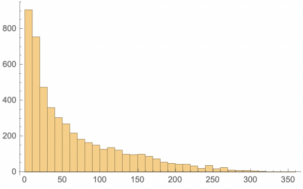
Figure 1: Distribution of the number of distinct irreps in the tensor decomposition of $R_{\vec{v}_{1}}\otimes R_{\vec{v}_{2}}$ for $A_{m}$ with randomized $1\leq m\leq 8$ and randomized ternary weight vectors $\vec{v}_{1,2}$. The horizontal axis denotes the length of $R_{\vec{v}_{1}}\otimes R_{\vec{v}_{2}}$ and the vertical axis denotes the corresponding frequency.

Let us next consider a simple binary classification problem using the data generated by LieART: can ML distinguish tensor decompositions of length $\geq 70$ and of length $<70$? The length $70$ is chosen since it splits the data rather evenly into around five thousands each. To uniformize the input vectors, for the rank $m<8$, we also pad both $\vec{v}_{1,2}$ to the right with $-1$ (a meaningless number in this context) and stack them on top of each other. Thus, our input is a $2\times 8$ matrix with integer entries for $1\leq m\leq 8$. This step is essential for using a single NN for learning data for Lie algebras of varying ranks (it is for $A_{m},1<m<8$ here). For the majority of our experiments, we use a feed-forward neural network classifier built in $\mathtt{Mathematica}$ with the architecture shown in Figure 2.

Figure 2: The neural network architecture. $S$ is the softmax activation and $D$ is a dropout layer with probability $0.2$. The hidden-layer neurons $(1,2)$ and $(4,5)$ are fully connected and sigmoid activated.

We also reproduced these results with a similar 2-layer architecture on $\mathtt{Keras}$ keras , with $\mathtt{selu}$ activated neurons to obtain similar accuracy and confidence. Finally, we need to ensure that the last softmax is rounded to 0 or 1 according to our binary categories.

The results of our training and learning for $A_{m}$ are depicted in figure 3. The data was partitioned into 64% training, 16% validation, and 20% test splits. The network was trained on the training and validation sets and the test set was used purely for evaluating the trained network. The plots show a steady lowering in both the error-rate and loss-function as we increase the number of rounds of training and validation. We achieved accuracy 0.969, confidence 0.930, 5% error rate, and 0.1 loss function within one minute by training for 100 epochs using learning rate $10^{-3}$, ADAM optimizer; which is excellent indeed. Throughout this letter, we will use “accuracy” to mean percentage agreement of predicted and actual values. In addition, in discrete classification problems it is also important to have a measure of “confidence” so that false positives/negatives can be noted. A widely used one is the so-called Matthews’ Phi-coefficient $\phi$ (essentially a signed square-root of the chi-squared of the contingency table) phi , which is $\lesssim 1$ for predictions with good confidence.

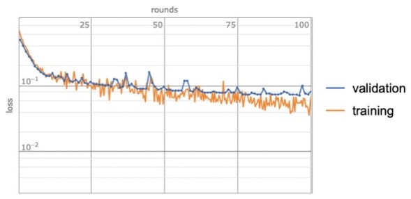
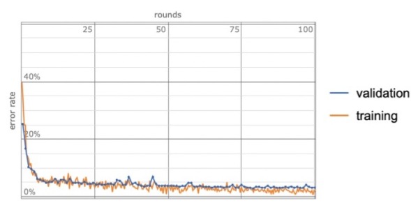
Figure 3: Loss-function (top), and error-rate (below) for training and validation for $A_{m}$ are plotted against number of epochs.

The above experiment was also carried out with other classical, as well as exceptional Lie algebras with comparable success. The results are given in table 1. We generated the same data size as in the $A_{m}$ case, i.e. 5000, and used the same cap on the maximum dimension of the irreps (10,000). In contrast, though the dimension cap for exceptional groups was set to 120,000, it yielded far fewer data points. The lengths we split the data-sets on were chosen to generate a balanced data-set in each case. The accuracy of ML prediction was above .95 for each of these cases.

Group	Data Size	Splitting Length	Accuracy	Confidence
$A_{m}$	5000	70	0.969	0.930
$B_{m}$	5000	40	0.959	0.878
$C_{m}$	5000	40	0.969	0.921
$D_{m}$	5000	35	0.965	0.908
$G_{2}$	1275	110	0.946	0.891
$E_{6}$	903	30	0.898	0.795

Table 1: The binary classification of product decomposition lengths. The splitting lengths yield a balanced dataset.

The relatively lower accuracy for $E_{6}$ is caused by the low number of points available at low dimensions due to its relatively high rank: 903 data points below dimension of 120,000. Raising the dimension cap would improve the machine-learning, bringing it up to par with others, however the corresponding data generation using LieART would take days.

We also note that partitioning the data-sets at the ‘midpoint’ to generate balanced data-sets as we have done above is by no means necessary. As an example, we explored this classification problem for the $A_{m}$ algebras but now organizing the data into partitions of varying lengths, viz. 20/80 through to 80/20. Here by a partition of length 20/80 we mean that a ‘cutoff’ decomposition length was chosen such that 20% of the decomposition lengths in the dataset are below this length, i.e. are denoted by the target variable $\mathrm{Y}=0$ and the remaining 80% are above, and hence denoted by $\mathrm{Y}=1$. In every case the Matthews’ Phi-coefficient remains close to 1. In particular, for the 20/80 and 80/20 partition it is 0.98.

We can take this experiment one step further and train the neural net on low dimensional tensor decomposition data, then test its performance on higher dimensional cases. If successful this would immensely reduce the computation time. For example, obtaining the length of decomposition for two $A_{6}$ weight vectors $\vec{v}_{1}=\vec{v}_{2}=(2,2,2,2,2,2)$ by brute force takes over 15 minutes on LieART while machine learning should estimate the length in a matter of seconds.

We retrained the NN in figure 2 on the same data for the classical and $G_{2}$ algebras generated by LieART for the previous experiment. However, the training set is now restricted to have both input weight vectors of dimension less than certain cut-off value, here taken to be 2,000. The trained neural network was subsequently evaluated on the test dataset consisting of input weight vectors of dimension ranging between 2,000 and 10,000. Our results are presented in Table 2 and Figure 4.

Group Train/Val Accuracy Test Accuracy Confidence $A_{m}$ 0.974/0.957 0.961 0.907 $B_{m}$ 0.972/0.963 0.957 0.845 $C_{m}$ 0.969/0.970 0.892 0.792 $D_{m}$ 0.971/0.940 0.956 0.817 $G_{2}$ 0.969/0.963 0.968 0.922 $E_{6}$ 0.963/0.947 0.875 0.751

Table 2: Training on low dimensional irreps, and testing on high dimensional ones.

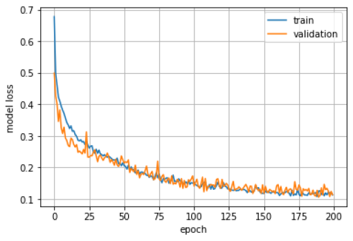
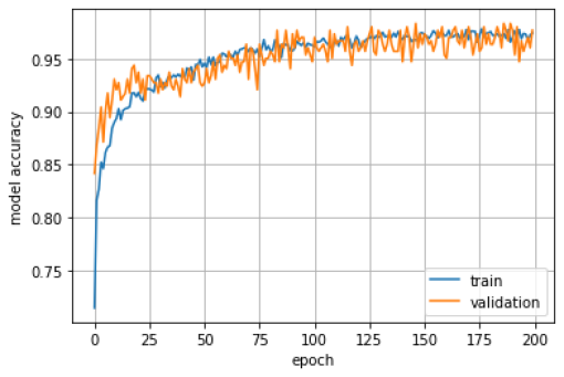
Figure 4: Loss-function (top), and model accuracy (below) for training on $A_{m}$ irreps, plotted against number of epochs.

II.1.2 Beyond Binary Classification

We now move beyond the simpler binary classification experiments done previously to a multi-class classification task, with the aim of predicting a range for the length of the product decomposition as opposed to the over/under estimates obtained above. For definiteness, let us take the $A_{m}$ data and classify it into five classes, depending on whether the length of the product decomposition lies in the ranges 0 to 10, 10 to 25, 25 to 55, 55 to 115 and greater than 115. Figure 5 shows a histogram with the class populations, and the training curves are displayed in Figure 6.

Figure 5: Class Populations of length bins for $A_{m}$ irreps.

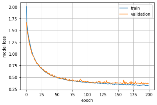
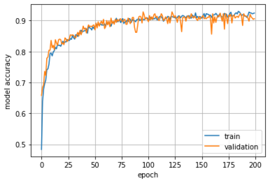
Figure 6: Training curves for the quinary classification problem for $A_{m}$, plotted against number of epochs.

The neural network reaches a $\phi$-coefficient of 0.917 on the test set, and the confusion matrix is given by

$$\begin{pmatrix}96&3&0&0&0\\ 1&92&3&0&0\\ 0&2&109&4&0\\ 0&0&7&86&7\\ 0&0&0&6&84\end{pmatrix}$$ (II.4)

II.2 Branching Rules

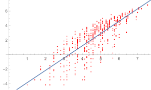
Figure 7: Plot and fit of log of the time in seconds of the branching of irreps of $SU(5)$ versus the length of the weight-vector.

The next task on which we train our neural network of Figure 2 is to learn about the branching rules for Lie algebras. Suppose we take a weight-vector of $SU(5)$, and restrict its entries from 0 to 4 (i.e., as quinary 4-vectors). Even though this may look rather harmless, the dimension of the corresponding irrep ranges from 1 for $\vec{0}$, to 9765625 for $\vec{4}$. When we decomposed these irreps of $SU(5)$ to those of its maximal sub-algebra $SU(3)\times SU(2)\times U(1)$, and found their explicit branching products, the time taken on LieART was easily seen to be exponential. In figure 7, we plot the log of the time taken in seconds, versus the length of the weight-vector. The best fit is the line $-5.54361+1.69186x$. By extrapolation, the single irrep of $SU(5)$ corresponding to weight vector $\overrightarrow{10}$ would take over 20 years just to compute its branching products into $SU(3)\times SU(2)\times U(1)$.

In the rest of this section, we shall show the efficacy of using ML to predict presence/absence of any given representation of the maximal sub-algebra in a given irrep of $SU(5)$ and $G_{2}$ algebras. For concreteness, we look for bi-fundamental representations of $SU(3)\times SU(2)$ (with arbitrary values of $U(1)$ charges) in any given $SU(5)$ irrep. In the $G_{2}$ case, we restrict ourselves to bi-fundamental representation of $SU(2)\times SU(2)$ maximal sub-algebra.

For the $SU(5)$ branching, we use first 800 irreps of smallest dimension as input vectors with binary output depending on presence/absence of a bi-fundamental rep of $SU(3)\times SU(2)$. The data was split into train/validation/test sets in the ratio 80/10/10. The neural network reached a test accuracy of 0.899 and a confidence of 0.813. The next best results were arrived at by a support vector classifier which reached an test accuracy of 0.838 and confidence of 0.677.

For the $G_{2}$ branching, we used 400 weight input vectors with dimensions below 4.7 million. Analogous to the $SU(5)$ case, the output was binary, depending on presence/absence of a bi-fundamental rep of $SU(2)\times SU(2)$. All classifiers, neural nets and otherwise, performed at the level of blind guessing in this case, which is possibly due to the relatively fewer input data as well as smaller number of features in the data.

III Outlook

Given the ubiquity of Lie algebras and groups in physics, let us end this letter with some comments about the vast possibilities in applications to physics of our results, exemplifying with two which immediately come to mind.

In scattering processes, given a pair of incoming particles transforming under the irreps of certain global symmetry group, the outgoing particles can be classified via their tensor decompositions. The tensor decomposition prediction and extrapolation results in section II.1 thus allow us to efficiently estimate the number of distinct outgoing particles. It would also be exciting to see if the NN upper bound estimate of the length of a given decomposition can help LieART package to work out its explicit terms within significantly shorter period.

Our choice of studying the branching of $SU(5)$ into its maximal subgroup $SU(3)\times SU(2)\times U(1)$ in section II.2 was phenomenologically motivated. This hopefully can lead to an useful algorithm for testing whether a field transforming under $SU(5)$ GUT gauge group can yield descendants transforming under standard model gauge groups upon spontaneous symmetry breaking. We hope this will be useful for particle physics model building purposes.