Efficient texture mapping via a non-iterative global texture alignment

Abstract

Texture reconstruction techniques generally suffer from the errors in keyframe poses. We present a non-iterative method for seamless texture reconstruction of a given 3D scene. Our method finds the best texture alignment in a single shot using a global optimisation framework. First, we automatically select the best keyframe to texture each face of the mesh. This leads to a decomposition of the mesh into small groups of connected faces associated to a same keyframe. We call such groups fragments. Then, we propose a geometry-aware matching technique between the 3D keypoints extracted around the fragment borders, where the matching zone is controlled by the margin size. These constraints lead to a least squares (LS) model for finding the optimal alignment. Finally, visual seams are further reduced by applying a fast colour correction. In contrast to pixel-wise methods, we find the optimal alignment by solving a sparse system of linear equations, which is very fast and non-iterative. Experimental results demonstrate low computational complexity and outperformance compared to other alignment methods.

Computing methodologiesComputer graphicsImage manipulationTexturing Computing methodologiesComputer graphicsShape modelingMesh models Computing methodologiesComputer graphicsGraphics systems and interfacesMixed / augmented reality

1 Introduction

Texture reconstruction is a fundamental problem of 3D computer vision with many applications in virtual and augmented reality [14] and interior design [17]. Thanks to commodity sensors and modern visual tracking systems, 3D geometry and texture can be easily reconstructed. However, with the presence of errors in camera poses and illumination changes, it may not result in a high quality reconstruction. In this work we focus on texture reconstruction problem as photometric information is visually more salient than geometry [8]. We assume that a 3D mesh is provided along with several keyframes and their associated camera poses.

Texture alignment can be seen as an image stitching problem in 3D between several keyframes, where moving any keyframe may impact several neighbours. Hence, an efficient method should find the optimal alignment by considering all keyframes at the same time. Such a method can be very slow and may trap in some local minimum. In this paper we find the global texture assignment using a non-iterative method, which exploits 3D feature matching. Our method has a very low computational complexity as it only requires solving a sparse system of linear equations. Figure 1 shows how visual seams, caused by errors in camera poses, are removed after applying the optimal alignment and colour correction.

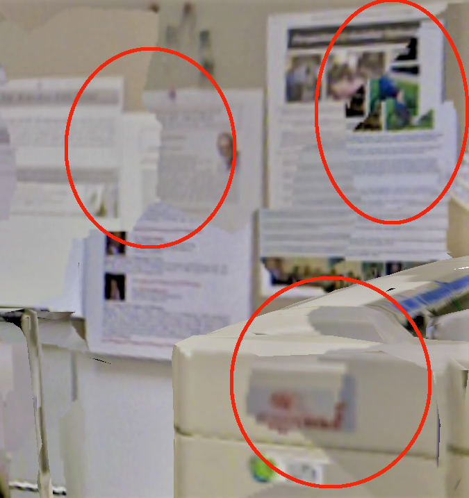
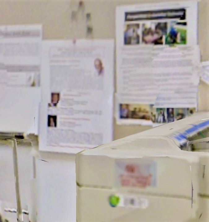
Figure 1: Texture reconstruction: $(left)$ direct mapping using closest keyframes; $(right)$ our result after alignment and colour correction.

2 State of the Art

Texture reconstruction is widely studied in both computer vision and graphics communities [6, 9]. Given a mesh and a camera trajectory, the first step consists of scoring the texture quality using the camera distance and angle [11]. Then, a greedy algorithm may be applied for texturing each region using the closest view. Markov Random Field (MRF), alternatively, proposes an optimal way that reduces seam effects in the texture map [8]. It decomposes the scene into small fragments, each textured by the best keyframe that is closer and more fronto-parallel (see Figure 2).

Illumination changes across the keyframes may lead to visual seams, which requires colour correction [16, 15]. In addition, there might be geometric misalignment between fragments due to the errors in camera pose estimation and geometry reconstruction [2]. The MRF formulation in [7] not only selects the best view per face, but also corrects the projection within $9$ possible translations. Optical flow between the overlapping images is used in [5] to warp input images and correct local misalignment.

Zhou et al. in [18] propose a method to jointly find the optimal camera poses and the best colour per vertex. It requires minimizing a non-linear least squares that converges slowly. Similarly, Fu et al. in  [6] present a two-step method for global and local texture alignment, where deformations per both fragment and vertex are permitted. Laplacian model is used in [12] to capture non-rigid deformations of keyframes and to obtain a better texture consistency along the fragment borders. However, both [12, 6] are iterative methods that get regularly stuck in local minimum. In the presence of large geometric errors, their correction methods fail to find the optimal alignment and generate some local texture distortions.

In a recent work, Lee et al. in [10] propose a real-time texture integration framework for on-line RGB-D scanning. In their fusion algorithm they update the texture map in every step of geometry fusion, which requires updating the camera motion field in a hierarchical manner. The photometric consistency of the texture and input images is evaluated in their texture-to-image registration step; therefore, the quality of texture reconstruction may degrade a lot in the presence of exposure changes and view-dependent appearance.

3 Proposed Texturing Pipeline

The input of the texture mapping consists of a 3D mesh with lists of vertices $\mathcal{V}$ and faces $\mathcal{F}$ in addition to several keyframes $\{I_{1},\dots,I_{N}\}$ and their poses. The proposed method, summarized in Algorithm 1, starts by extracting 3D feature points: for each keyframe we extract the 2D keypoints using SURF [4] and back-project them to 3D space using the virtual depth map obtained by rendering the mesh in the given keyframe pose.

1:  Input: 3D mesh, keyframes + poses, margin size.

2:  Step 0. 3D keypoint extraction:

3:  Extract and back-project keypoints for each keyframe.

4:  Step 1. View selection:

5:  Find the best keyframe per face.

6:  Step 2. Texture alignment:

7:  a. Construct the pose correction system:

8:  for every fragment border do

9:     i. Select visible keypoints within the margin.

10:     ii. Match the selected feature points.

11:     iii. Update the correction system for all matching pairs.

12:  end for

13:  b. Solve the system of equations to correct fragment poses.

14:  c. Build the texture atlas for the corrected poses & colours.

Algorithm 1 Texture reconstruction with alignment.

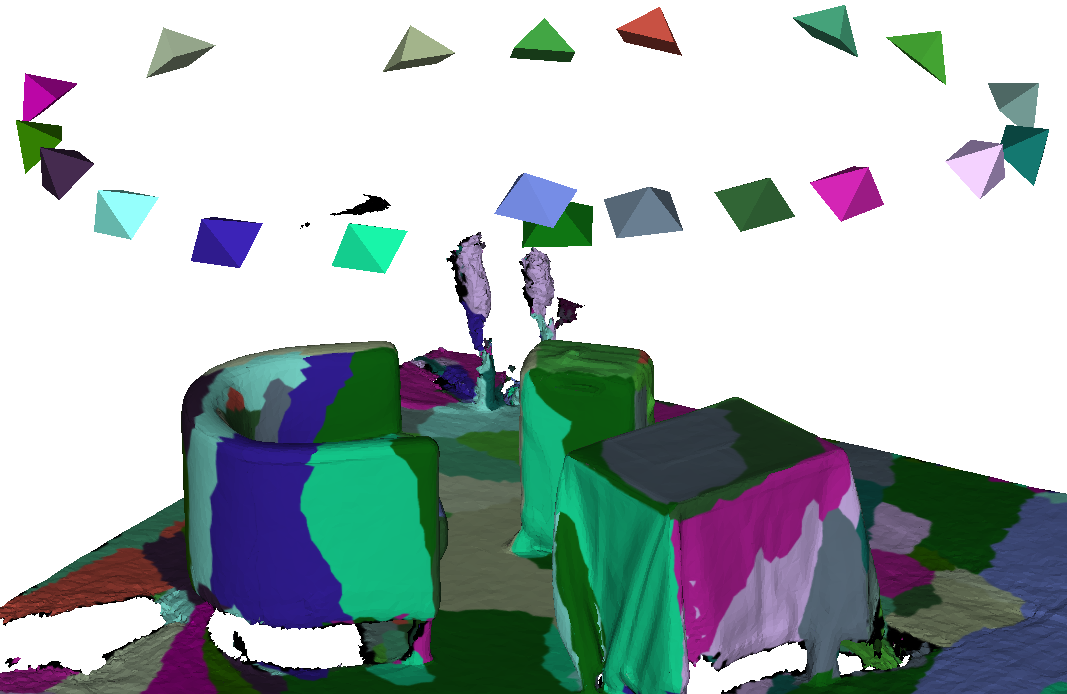
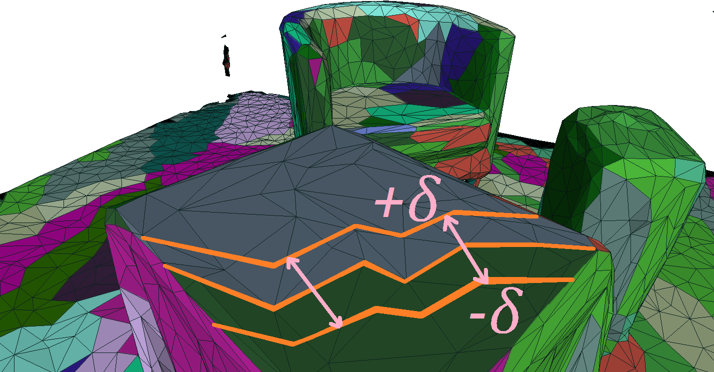
Figure 2: View selection: $(left)$ scene decomposed into fragments using automatic view selection; $(right)$ margin around a fragment border.

3.1 View Selection

In view selection, for each face, we aim at finding the keyframe that will provide the best texturing. Given the labeling $\mathbf{l}=\left(l_{f}\right)_{f\in\mathcal{F}}$ with $l_{f}\in\left[1,\dots,N\right]$, we consider the following objective function :

$$E\left(\mathbf{l}\right)=\sum_{f\in\mathcal{F}}{\psi_{f}\left(l_{f}\right)\ }+\lambda_{1}\sum_{\left(f,g\right)\in\mathcal{E}}{\varphi_{fg}\left(l_{f},l_{g}\right)},$$ (1)

where $\mathcal{E}$ is the set of neighbor faces and $\lambda_{1}$ is a positive parameter that weights the influence of the second term. The data term $\psi_{f}\left(l_{f}\right)$ measures the quality of the keyframe $I_{l_{f}}$ for texturing the face $f$ and the regularization term $\varphi_{fg}\left(l_{f},l_{g}\right)$ controls the texture smoothness between faces $f$ and $g$. In our implementation, we use the area of projection as the data term and the Potts model as the regularizer [15]. We minimize the global energy by applying graph cuts [3]. The resulting labeling decomposes the mesh into small fragments, a fragment being a set of connected faces with the same label.

3.2 Texture Alignment System

In this section we build an over-determined system of equations $\mathbf{A}_{pose}\boldsymbol{\Omega}=\mathbf{b}_{pose}$, where $\boldsymbol{\Omega}$ consists of all correction vectors $\boldsymbol{\omega}_{i}$ of each fragment $i$. Every correction vector $\boldsymbol{\omega}_{i}=[\alpha,\beta,\gamma,t_{x},t_{y},t_{z}]^{T}$ has $6$ parameters building a skew-symmetric matrix $\mathbf{T_{i}}$:

$$\mathbf{T}_{i}=\begin{pmatrix}1&-\gamma&\beta&t_{x}\\ \gamma&1&-\alpha&t_{y}\\ -\beta&\alpha&1&t_{z}\\ 0&0&0&1\end{pmatrix}.$$ (2)

For the sake of simplicity in the notations, let us note abusively $I_{i}$ the keyframe associated with fragment $i$. For every pair of neighboring fragments $i$ and $j$ we follow these steps to update the matrix $\mathbf{A}_{pose}$ and vector $\mathbf{b}_{pose}$:

i) Select relevant keypoints: First, we find all keypoints in $I_{i}$ and $I_{j}$ that fall inside a given margin around their common border (see Figure 2$(right)$). Moreover, we filter out those keypoints that are not visible in the other keyframe.

ii) Match selected keypoints: These two sets of keypoints are matched using FLANN [13]. 3D coordinates of keypoints are exploited as additional descriptors for discarding those far matches. Then, we obtain a set of pairs of 3D keypoints $\{(\mathbf{P}^{i}_{k},\mathbf{P}^{j}_{k})\}$ with weights $\{\mu_{k}\}$ that are higher close to the border (see Figure 3).

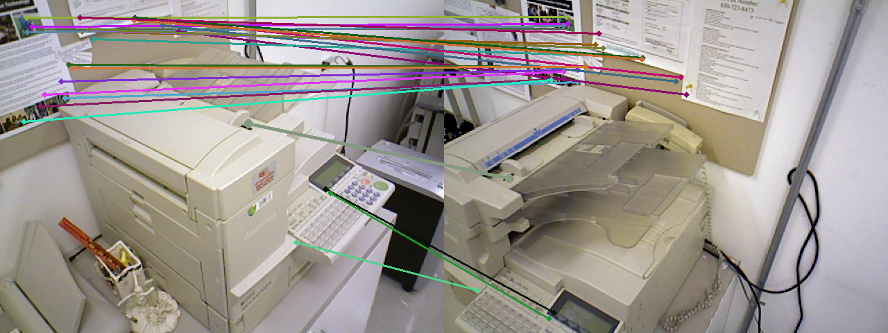
Figure 3: Geometry-aware matching around a fragment border.

iii) Update the pose correction system: These matching pairs must impact $\mathbf{T}_{i}$ and $\mathbf{T}_{j}$: the pose correction of the neighboring fragments. Ideally, $\mathbf{P}^{i}_{k}$ and $\mathbf{P}^{j}_{k}$ must get closer after applying these corrections:

$$\mathbf{P}^{i}_{k}+\mathbf{A}^{i}_{k}\boldsymbol{\omega}_{i}=\mathbf{P}^{j}_{k}+\mathbf{A}^{j}_{k}\boldsymbol{\omega}_{j},$$ (3)

where $\mathbf{A}^{i}_{k}$ is derived from $\mathbf{P}^{i}_{k}=(x_{k},y_{k},z_{k})$ as follows:

$$\mathbf{A}^{i}_{k}=\begin{pmatrix}0&z_{k}&-y_{k}&1&0&0\\ -z_{k}&0&x_{k}&0&1&0\\ y_{k}&-x_{k}&0&0&0&1\end{pmatrix}.$$ (4)

Then, every pair of matches adds $3$ constraints by copying $\mu_{k}\mathbf{A}^{i}_{k}$ and $-\mu_{k}\mathbf{A}^{j}_{k}$ to the associated columns of $\mathbf{A}_{pose}$ and by concatenating the vector $\mu_{k}(\mathbf{P}^{j}_{k}-\mathbf{P}^{i}_{k})$ to $\mathbf{b}_{pose}$.

Having considered all pairs of neighbouring fragments, the optimal alignment can be found by minimizing:

$$\varphi({\boldsymbol{\Omega}})=\|\mathbf{A}_{pose}\boldsymbol{\Omega}-\mathbf{b}_{pose}\|^{2}+\lambda_{2}\|\boldsymbol{\Omega}\|^{2},$$ (5)

where the regularization factor $\lambda_{2}$ controls the amount of correction. It leads to a sparse system of equations that can be quickly solved by QR factorization.

The optimal correction vector $\boldsymbol{\Omega}$ encodes the deformation matrices $\mathbf{T}_{i}$ for each fragment. Moreover, we apply colour correction [15] before copying the texture information from each keyframe to the final texture atlas (see Figure 5).

4 Experimental Results

The proposed method has been tested on several public data sets, where a raw mesh and multiple keyframes are provided. Figures 1, 4, 5 and the first two rows of Figure 6 illustrate the texturing results for Copyroom, Fountain and Lounge provided by [18]. In addition, we gathered our own data sets using a StructureIO mounted on an iPad Pro. The last four rows of Figure 6 are captured through our scanning platform.

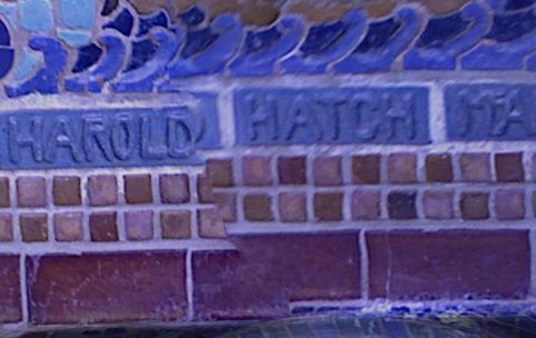
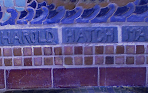
Figure 4: $(left)$ Iterative method, such as [12], may get trapped in a local minimum, $(right)$ while our method finds the global solution.

The amount of distortion in Figures 1 and 4 makes most pixel-wise or iterative methods, such as [6] and [12], get trapped in a local minimum. In contrast, our global optimization finds the optimal alignment over the whole set of texture fragments in a non-iterative way by solving a sparse system of linear equations.

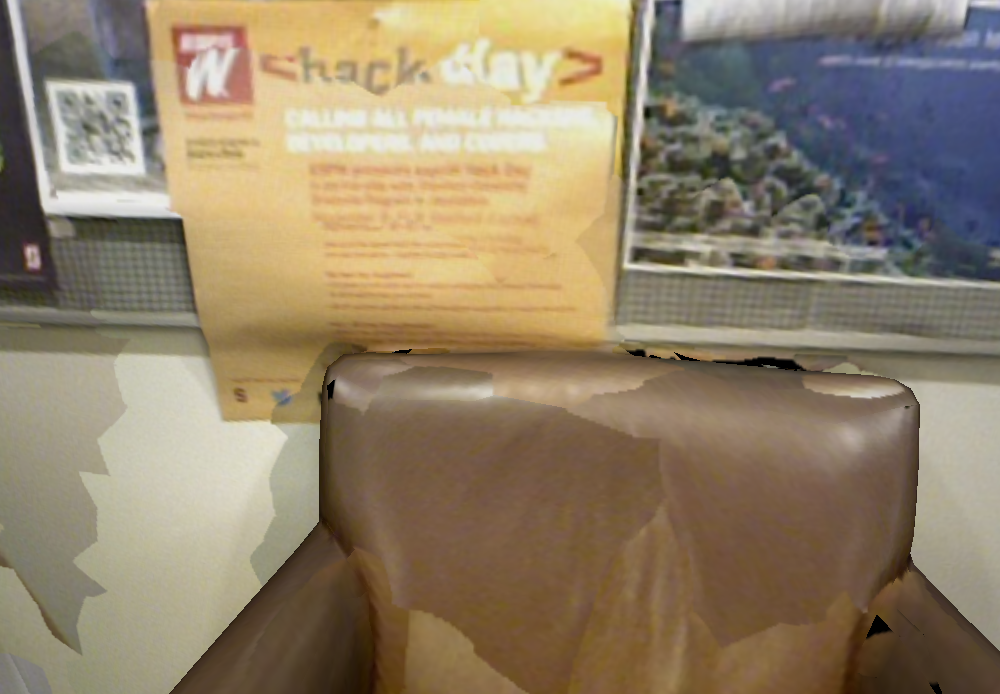
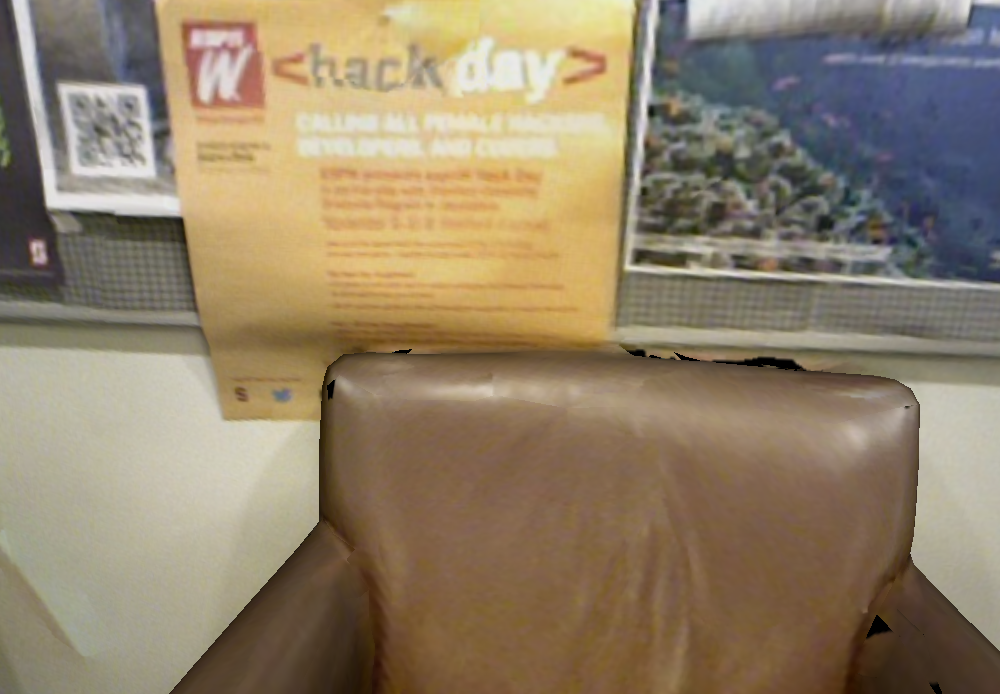
Figure 5: $(left)$ Input; $(right)$ colour correction and alignment applied.

Figure 6 presents comparisons of the method with several state of the art techniques. The results have been qualitatively compared with [1, 7, 16]. The far left column highlights the regions where misalignment and illumination changes happen. In most of cases our method provides the best quality reconstruction. Table 1 states the details about the scene geometry as well as the CPU timing for different steps. It includes the two main steps of our algorithm for view selection and texture alignment, where global optimization problems are solved by MRF and LS.

Please notice that if timing for our unoptimized step 0 may appear quite long, it is directly related to the chosen type of features to be extracted and could be accelerated preferring ORB to SURF for example. Since we use geometric clues, such as 3D positions of features, for matching the performance does not change by switching between descriptors. Note also that this pre-processing step is highly parallelizable and would deserve a GPU implementation. This implementation change is still an on-going work so that total timings should be very carefully compared.

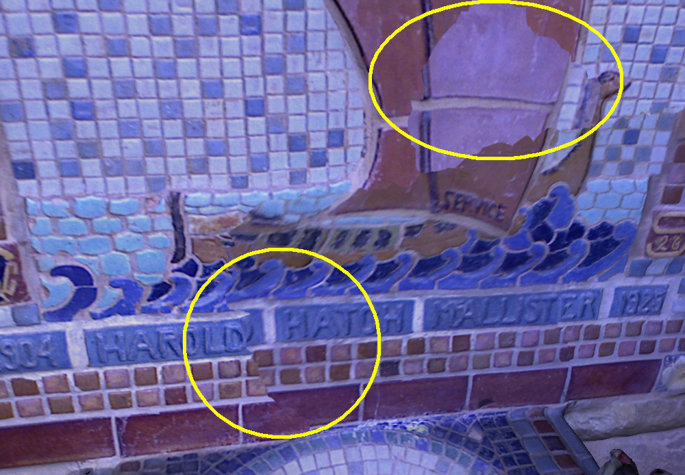
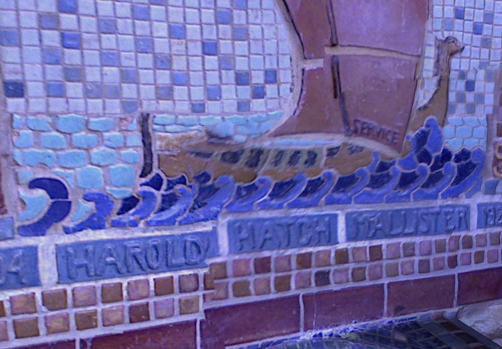
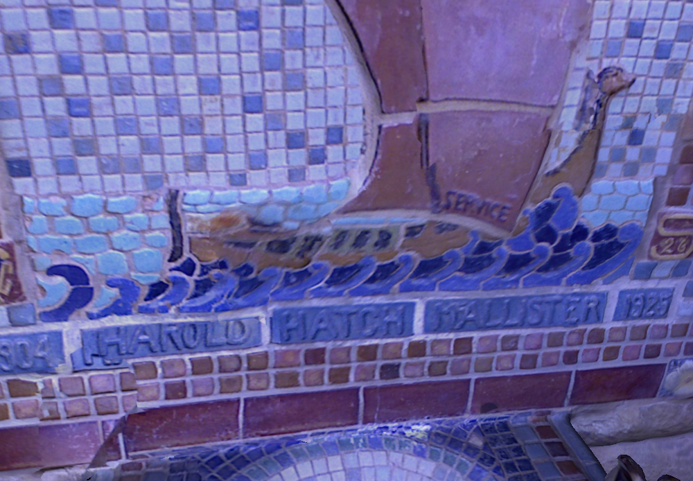
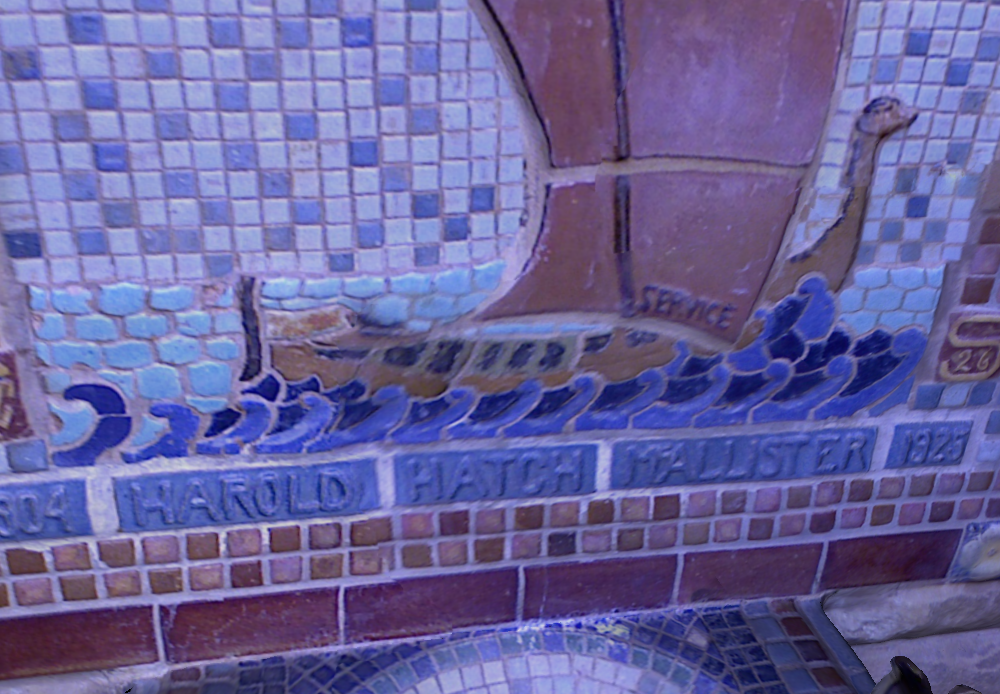
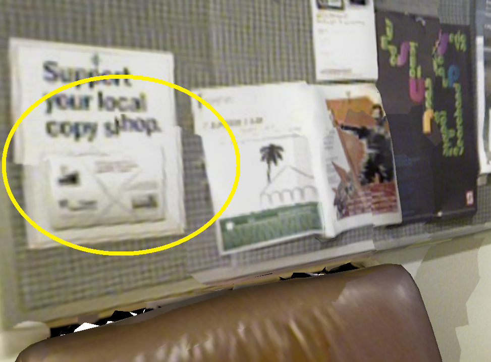
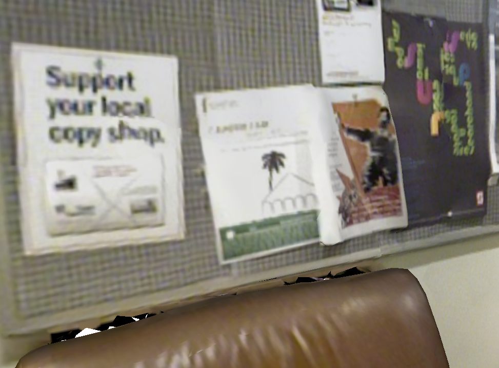
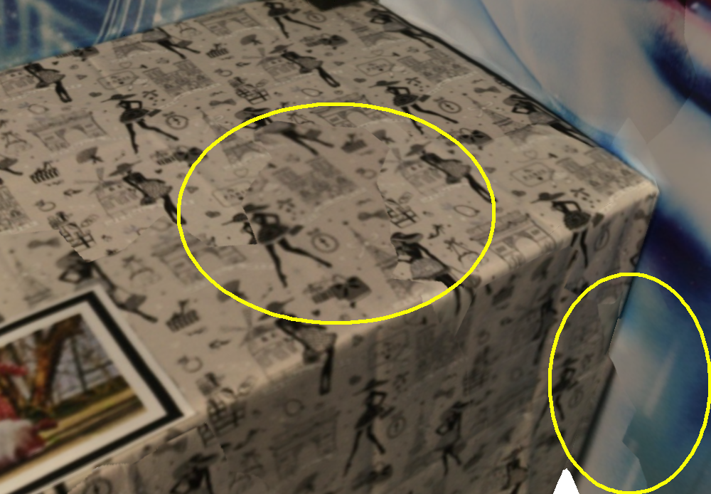
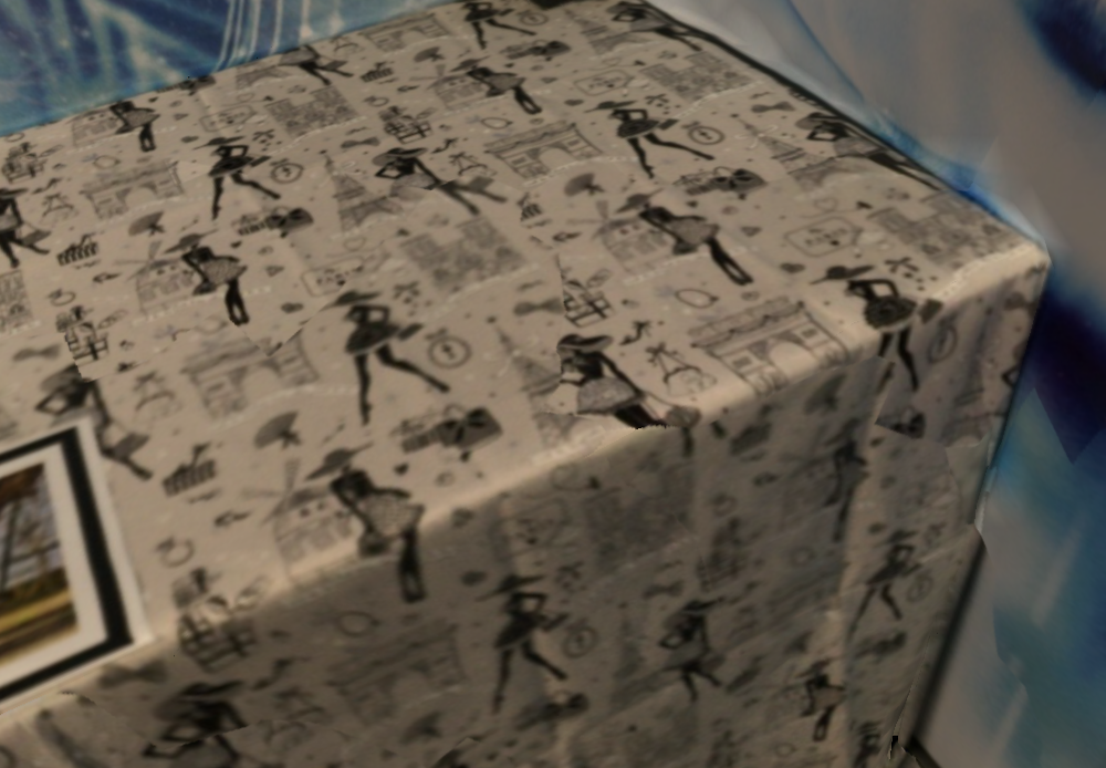
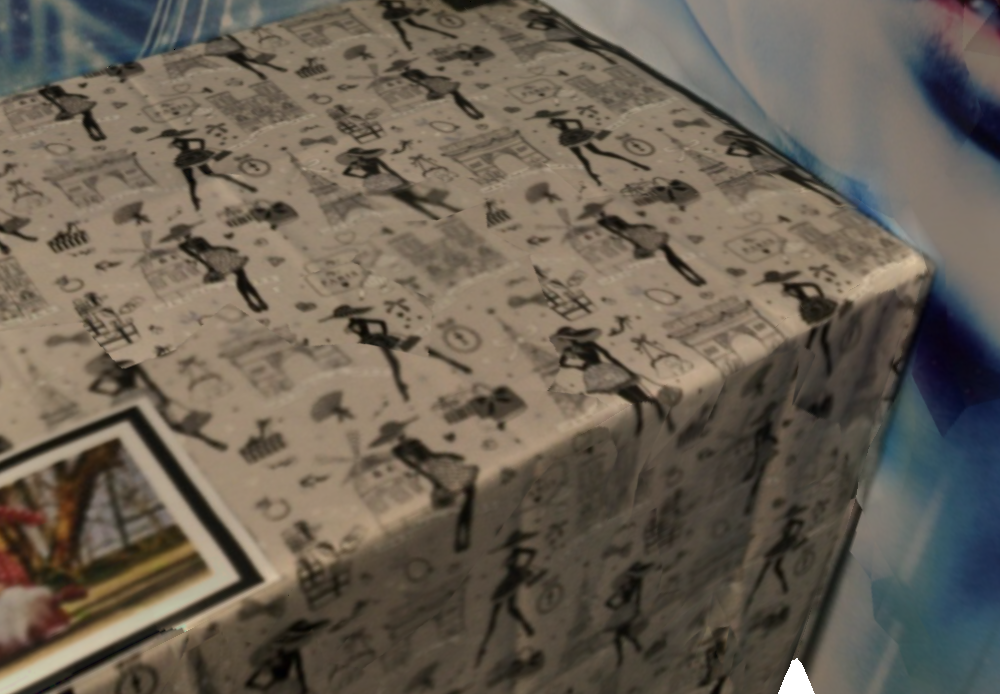
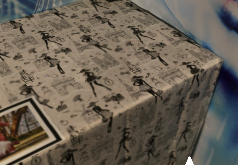
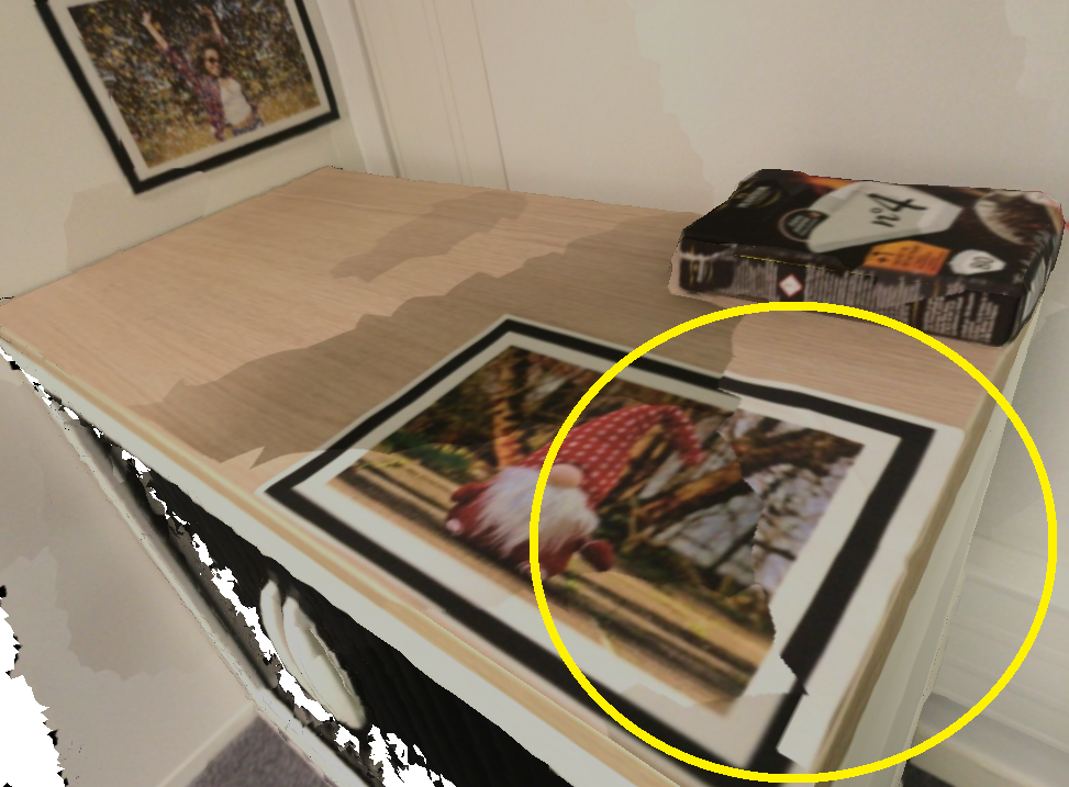
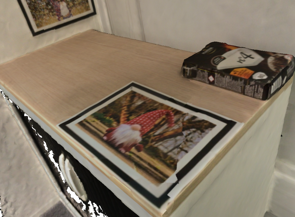
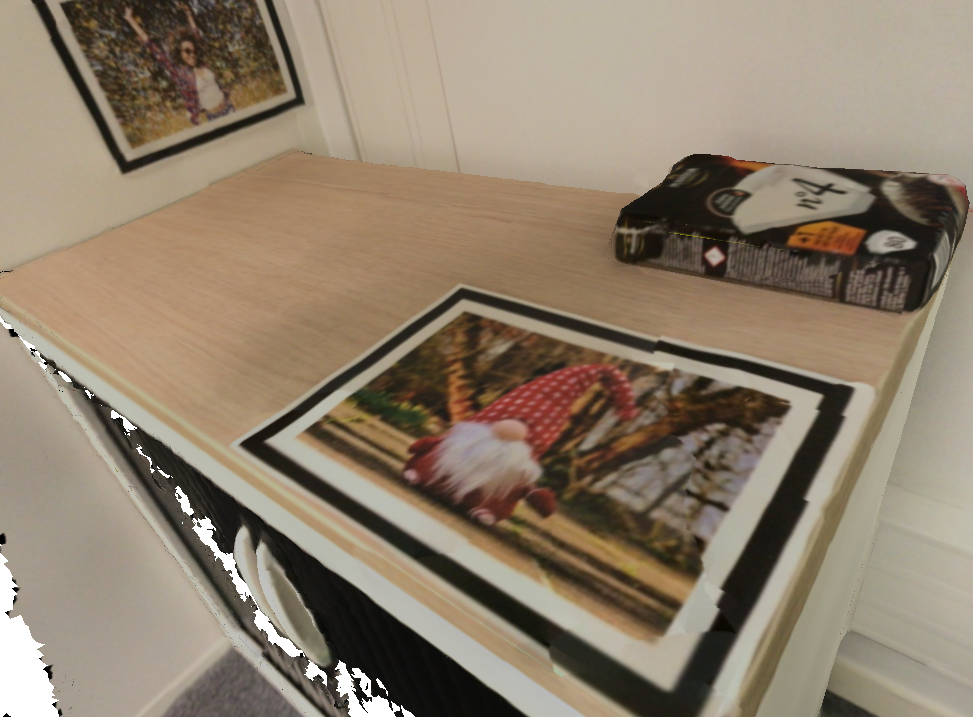
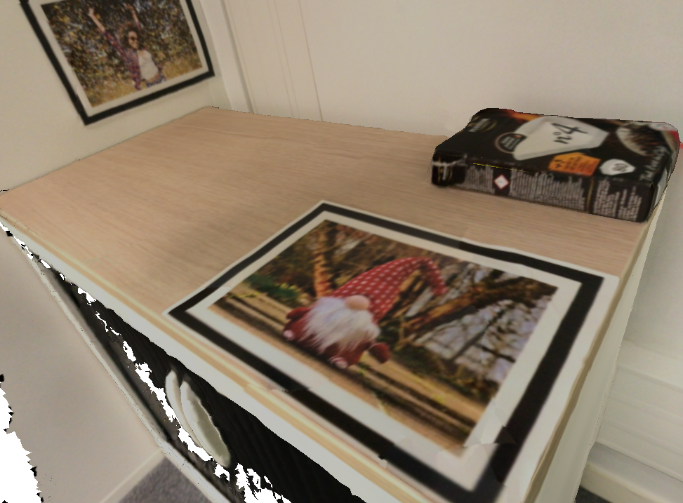
(a)	(b)	(c)	(d)

Figure 6: Comparisons: $(a)$ direct texture mapping before the colour correction [16]; $(b)$ method in [1] encouraging colour consistency; $(c)$ method in [7] applying pose correction per face; $(d)$ our results after pose and colour correction.

Fig.	$|\mathcal{F}|$	$N$	[1]	[7]	unoptim.	our	our
					step0		step2
6-$1$	117$k$	30	19.69	196.17	68.81	3.28	4.08
6-$2$	128$k$	55	17.11	206.09	14.74	10.06	0.81
6-$3$	20$k$	11	0.52	7.87	20.03	0.10	0.79
6-$4$	81$k$	13	3.72	41.55	11.72	0.89	0.53
6-$5$	105$k$	7	1.84	27.55	11.09	0.71	0.54
6-$6$	87$k$	11	2.23	23.8	10.57	0.77	0.39

Table 1: CPU timing (in seconds) for steps 0-2 of Algorithm 1, and for the methods presented in [1] and [7] as well. $|\mathcal{F}|$ and $N$ represent the number of faces and keyframes, respectively.

5 Conclusion

In this work a novel technique for global texture reconstruction has been presented. Our method is non-iterative and it exploits a geometry-aware feature matching between the keyframes. Moreover, it has a very low computational complexity as it requires solving a sparse system of equations. The margin size around the fragment borders defines how big the overlapping region can be. The qualitative results together with the low computational complexity, and the explicit hyper-parameters prove our method to be efficient and quite fast for texture reconstruction.

References

- [1] C. Allène, J.-P. Pons, and R. Keriven. Seamless image-based texture atlases using multi-band blending. In Int. Conf. on Pattern Recognition, pp. 1–4, 2008.
- [2] S. Bi, N. K. Kalantari, and R. Ramamoorthi. Patch-based optimization for image-based texture mapping. ACM Trans. on Graphics, 36(4), 2017.
- [3] Y. Boykov, O. Veksler, and R. Zabih. Fast approximate energy minimization via graph cuts. IEEE Transactions on pattern analysis and machine intelligence, 23(11):1222–1239, 2001.
- [4] M. Brown and D. G. Lowe. Automatic panoramic image stitching using invariant features. Int. Jour. Computer Vision, 74(1):59–73, 2007.
- [5] M. Dellepiane, R. Marroquim, M. Callieri, P. Cignoni, and R. Scopigno. Flow-based local optimization for image-to-geometry projection. IEEE Trans. Visualization Computer Graphics, 18(3):463–474, 2012.
- [6] Y. Fu, Q. Yan, L. Yang, J. Liao, and C. Xiao. Texture mapping for 3D reconstruction with RGB-D sensor. In Conf. Computer Vision Pattern Recognition, 2018.
- [7] R. Gal, Y. Wexler, E. Ofek, H. Hoppe, and D. Cohen-Or. Seamless montage for texturing models. In Computer Graphics Forum, pp. 479–486, 2010.
- [8] J. Huang, A. Dai, L. Guibas, and M. Nießner. 3DLite: towards commodity 3D scanning for content creation. ACM Trans. on Graphics, 2017.
- [9] J. Kim, H. Kim, J. Park, and S. Lee. Global texture mapping for dynamic objects. In Computer Graphics Forum, pp. 697–705, 2019.
- [10] J. H. Lee, H. Ha, Y. Dong, X. Tong, and M. H. Kim. Texturefusion: High-quality texture acquisition for real-time rgb-d scanning. In IEEE Conf. Computer Vision Pattern Recognition, pp. 1272–1280, 2020.
- [11] V. Lempitsky and D. Ivanov. Seamless mosaicing of image-based texture maps. In IEEE Conf. on Computer Vision and Pattern Recognition, pp. 1–6, 2007.
- [12] W. Li, G. Huajun, and Y. Ruigang. Fast texture mapping adjustment via local/global optimization. IEEE Trans. on Visualization and Computer Graphics, 2018.
- [13] M. Muja and D. G. Lowe. Fast approximate nearest neighbors with automatic algorithm configuration. In A. Ranchordas and H. Araújo, eds., VISAPP, pp. 331–340. INSTICC Press, 2009.
- [14] G. Queguiner, M. Fradet, and M. Rouhani. Towards mobile diminished reality. In IEEE Int. Symposium on Mixed and Augmented Reality, ISMAR 2018 Adjunct, Munich, Germany, pp. 226–231, 2018.
- [15] M. Rouhani, M. Fradet, and C. Baillard. A multi-resolution approach for color correction of textured meshes. In IEEE Conference on 3D Vision., pp. 71–78, 2018.
- [16] M. Waechter, N. Moehrle, and M. Goesele. Let there be color! large-scale texturing of 3D reconstructions. In European Conference on Computer Vision, pp. 836–850, 2014.
- [17] E. Zhang, M. F. Cohen, and B. Curless. Emptying, refurnishing, and relighting indoor spaces. ACM Trans. on Graphics, 35(6):174, 2016.
- [18] Q.-Y. Zhou and V. Koltun. Color map optimization for 3D reconstruction with consumer depth cameras. ACM Transactions on Graphics, 33(4):155, 2014.