Neural Ordinary Differential Equations on Manifolds

Abstract

Normalizing flows are a powerful technique for obtaining reparameterizable samples from complex multimodal distributions. Unfortunately current approaches fall short when the underlying space has a non trivial topology, and are only available for the most basic geometries. Recently normalizing flows in Euclidean space based on Neural ODEs show great promise, yet suffer the same limitations. Using ideas from differential geometry and geometric control theory, we describe how neural ODEs can be extended to smooth manifolds. We show how vector fields provide a general framework for parameterizing a flexible class of invertible mapping on these spaces and we illustrate how gradient based learning can be performed. As a result we define a general methodology for building normalizing flows on manifolds.

1 Introduction

Recently Chen et al. (2018) showed how to effectively integrate Ordinary Differential Equations (ODE) with Deep Learning frameworks. Ubiquitous in all fields of science, differential equations are the main modelling tools for physical processes. In deep learning their introduction was initially motivated from the observation that the popular residual network (ResNet) architecture can be interpreted as an Euler discretization step of a differential equation (Haber & Ruthotto, 2017). Instead of relying on discretized maps, Chen et al. (2018) proposed to directly model the continuous dynamics using vector fields in $\mathbb{R}^{n}$. A vector field, through its associated ODE, indicates for every point an infinitesimal displacement change, and therefore implicitly describes a map from the space to itself called a flow. While the flow can be practically computed using numerical ODE solvers, the key observation of Chen et al. (2018) is that we can threat the ODE solution as a black-box. This means that in the backward pass we do not have to differentiate through the operations performed by the numerical solver, instead Chen et al. (2018) propose to use the adjoint sensitivity method (Pontryagin et al., 1962). Closely related with the Pontryagin Maximum Principle, one of the most prominent results in control theory, the adjoint sensitivity method allows to compute vector-Jacobian product of the ODE solutions with respect of its inputs. This is done by simulating the dynamics given by the initial ODE backwards, augmenting it with a linear differential equation, which intuitively can be thought of as a continuous version of the usual chain rule.

Neural ODEs found one of their major applications in the context of normalizing flows (Grathwohl et al., 2019; Finlay et al., 2020). Normalizing flows are a general methodology for defining complex reparameterizable densities by applying a series of diffeomorphism to samples from a (simple) base distribution (Rezende & Mohamed, 2015). The resulting density at the transformed points can be computed using the change of variable formula. Flows defined by vector fields are particularly amenable for this task, as for every time interval the ode solution defines a diffeomorphism. In this case, the change change of density is given simply by integrating the divergence of the vector field along integral curves.

As many real word problems are naturally defined on spaces with a non-trivial topology, recently there has been a great interest in building probabilistic deep learning frameworks that can works on manifolds different from the Euclidean space (Davidson et al., 2018; Falorsi et al., 2018, 2019; Pérez Rey et al., 2019; Nagano et al., 2019). For this objective the possibility of defining complex reparameterizable densities on manifolds through normalizing flows is of central importance. However as of today there exist few alternatives, mostly limited to the most basic and simple topologies.

The main obstacle for defining normalizing flows on manifolds is that there is no general methodology for parameterizing maps $F:M\to N$ between two manifolds. Neural networks can only accomplish this for the the Euclidean space, $\mathbb{R}^{n}$. In this work we propose to use vector fields on a manifold $M$ as a flexible way to parameterize diffeomorphic maps from the manifold to itself. As a vector fields defines an infinitesimal displacement on the manifold for every point, they naturally give rise to diffeomorphisms without needing to impose further constraints. In addition, there exist decades old research on how to numerically integrate ODEs on manifolds.

We start in Section 2 by delineating how vector fields and ODEs on a manifold $M$ can be defined in the context of differential geometry. We then explain how vector fields naturally give rise, through their associated flow, to diffeomorphisms on $M$. In Section 3 we describe how the adjoint sensitivity method can be generalized to vector fields on manifolds in the context of geometric control theory (Agrachev & Sachkov, 2013). This highlights important connections with symplectic geometry and the Hamiltonian formalism. Similarly as in the adjoint method in the Euclidean space, to backpropagate through the flow defined by a vector field we have to solve an ODE in an augmented space. In this case the ODE is given by a vector field on the cotangent space $T^{*}M$, called cotangent lift, which is a lift of the original vector field on $M$. In Section 4 we demonstrate how flows defined by vector fields allow to define continuous normalizing flows on manifold. As a proof of concept we show how the defined framework can be used to model complex multimodal densities on the hypersphere in Appendix A and provide practical advice on how to parameterize vector fields on a manifold using neural networks in Appendix B.

2 Vector fields and flows on manifolds

Throughout the paper $M$ will be a $n$-dimensional smooth manifold. Vector fields are the mathematical object that allows us to generalize the concept of ODEs to manifolds. A smooth vector field $X$ is defined as a smooth section of the tangent bundle $X\in\Gamma^{\infty}\left(M,TM\right)$. A smooth time dependent vector field is a smooth function $X:\mathbb{R}\times M\to TM$ such that $\forall t\in\mathbb{R}$, $X_{t}:=X(t,\cdot)\in\Gamma^{\infty}\left(M,TM\right)$ is a smooth vector field.

Definition 1.

Let $X:\mathbb{R}\times M\to TM$ be a smooth time dependent vector field and $J\subseteq\mathbb{R}$ an interval. A curve $\gamma:J\to M$ is an integral curve of $X$ if:

$$\dot{\gamma}(t)=X(t,{\gamma(t)})\quad\forall t\in J$$ (1)

We call maximal integral curve an integral curve that cannot be extended to a larger interval $J$.

Writing Equation (1) in a local smooth chart we find that it is equivalent to (locally) solving a system of ODEs. We can then apply the existence and uniqueness theorem to show that every smooth vector field always admits integral curves:

Theorem 1 (Theorem 2.15 in (Agrachev et al., 2019)).

Let $X$ a smooth time dependent vector field, then for any point $(t_{0},p_{0})\in\mathbb{R}\times M$ there exist a unique maximal integral curve $\gamma:t_{0}\in J\to M$ with starting point $q_{0}$, and starting time $t_{0}$ denoted by $\gamma(t;t_{0},q_{0})$. We call $\gamma$ a solution of the Cauchy problem:

$$\left\{\begin{array}[]{l}\dot{q}(t)=X(q(t))\\ q(t_{0})=q_{0}\end{array}\right.$$ (4)

Moreover the map $(t_{0},q_{0})\to\gamma(t;t_{0},q_{0})$ is smooth on a neighborhood of $(t_{0},q_{0})$.

A time-dependent vector field is complete if for every $(t_{0},q_{0})\in\mathbb{R}\times M$, the maximal solution $\gamma(t;t_{0},q_{0})$ of the Cauchy problem is defined on all $\mathbb{R}$.

Through integral curves, vector fields on manifolds give us a flexible and convenient way of defining maps from $M$ to itself. Restricting to the time independent case, this means considering the family of maps $\phi_{X}^{t}:M\to M,\quad\phi_{X}^{t}(q)=\gamma(t;0,q)$ where $t\in\mathbb{R}$. In this case we say that the vector field generates a flow.

Definition 2.

A smooth flow is a smooth left $\mathbb{R}$-action on a manifold $M$; that is, a family of smooth diffeomorphisms $\phi^{t}:M\to M,\forall t\in\mathbb{R}$ satisfying the following properties for all $s,t\in\mathbb{R}$ and $q\in M$:

$$\phi^{0}=\text{Id},\quad\phi^{t}\circ\phi^{s}(q)=\phi^{t+s}\ \forall t,s\in\mathbb{R}$$ (5)

Every smooth flow $\phi$ uniquely generates a smooth complete vector field $X$ by $X_{q}=\frac{d}{dt}\bigr{|}_{t=0}\phi^{t}(q)\quad\forall q\in M$ Conversely every complete smooth vector field generates smooth flow $\{\phi_{X}^{t}\}_{t\in\mathbb{R}}$ through its integral curves. This result is known as the Fundamental Theorem of Flows.

For time dependent vector field we have to take into account the additional time dependence, we therefore have time dependent flows

Definition 3.

A time dependent smooth flow on a smooth manifold is a two parameter family of diffeomorphism $\{\phi^{t_{1},t_{0}}\}_{t_{0},t_{1}\in\mathbb{R}}$, $\phi^{t_{1},t_{0}}:M\to M,\forall t_{0},t_{1}\in\mathbb{R}$ that satisfy the following conditions:

$$\phi^{t,t}=Id,\quad\phi^{r,s}\circ\phi^{s,t}=\phi^{r,t}\quad\forall t,s,r\in\mathbb{R}$$ (6)

Similarly as the time independent case we have that a time dependent complete smooth vector field uniquely generates a time dependent smooth flows and vice versa.

Summing up we have seen how vector fields naturally allow us define maps on a generic smooth manifold $M$. We refer to (Lee, 2013) for proofs and additional results on vector fields and flows on manifolds.

3 Cotangent lift

Let $X\in\Gamma^{\infty}\left(M,TM\right)$ a complete smooth vector field and $\{\phi^{t}_{X}\}_{t\in\mathbb{R}}$ its generated flow. We are interested in differentiating through $\phi^{t}_{X}:M\to M$. In differential geometry this corresponds to computing the pullback map $(\phi^{t}_{X})^{*}:T^{*}M\to T^{*}M$, where $T^{*}M$ is the cotangent bundle of $M$. The key observations of the adjoint sensitivity method is that in $M=\mathbb{R}^{n}$ this quantity can be computed simulating the reverse dynamics of $X$, augmenting it with an additional linear ODE called the adjoint equation. We will show how to generalize this method for vector fields on an arbitrary smooth manifold $M$. Consider the family of maps:

$$\left(\phi^{t}_{-X}\right)^{*}:T^{*}M \to T^{*}M\qquad\forall t\in\mathbb{R},$$ (7)

$$p_{q} \mapsto\left(\left(\phi^{t}_{-X}\right)^{*}p\right)_{\phi^{t}_{X}\left(q\right)}$$ (8)

Using the properties of the pullback and the fact that $\{\phi_{-X}^{t}\}_{t\in\mathbb{R}}$ is a flow it is easy to show that the family $\{\left(\phi^{t}_{-X}\right)^{*}\}_{t\in\mathbb{R}}$ defines a flow on $T^{*}M$. Following Section 2 there exists a unique vector field $X^{T^{*}}\in\Gamma^{\infty}\left(T^{*}M,TT^{*}M\right)$ on the cotangent bundle that generates this flow, this vector field is called the cotangent lift of $X$ (Bullo & Lewis, 2004):

$$X^{T^{*}}_{p_{q}}=\frac{d}{dt}\biggr{|}_{t=0}\left(\left(\phi^{t}_{-X}\right)^{*}p\right)_{\phi^{t}_{X}\left(q\right)}\quad\forall p_{q}\in M$$ (9)

This means that given the cotangent vector $p_{q}\in T_{q}^{*}M$, to compute the pullback of $p_{q}$ by $\phi_{X}^{t}$ we can solve the Cauchy problem defined by $-X^{T^{*}}$ with starting point $p_{q}$. The cotangent lift has the following important properties:

Property 1.

$X^{T^{*}}$ is a Hamiltonian vector field with respect to the canonical symplectic structure of the cotangent bundle $T^{*}M$. The Hamiltonian that generates $X^{T^{*}}$ is $H_{X}(p_{q})=p_{q}\left(X_{q}\right)$. We therefore have:

$$X^{T^{*}}\lrcorner\,\omega=dH_{X},$$ (10)

where $\omega$ is the canonical symplectic form on $T^{*}M$

Property 2.

$X^{T^{*}}$ is a linear vector field on the fibers of $T^{*}M$. That is, given $p_{q},p^{\prime}_{q}\in T^{*}_{q}M$, and $a,b\in\mathbb{R}$ it holds that $X^{T^{*}}(a\!\cdot\!p_{q}+b\!\cdot\!p^{\prime}_{q})=a\!\cdot\!X^{T^{*}}(p_{q})+b\!\cdot\!X^{T^{*}}(p^{\prime}_{q})$.

This fundamentally descends because the pullback map is fiberwise linear.

Property 3.

$X^{T^{*}}$ is a lift of $X$. That is $d\pi_{M}(X^{T^{*}}_{p_{q}})=X_{q},\forall p_{q}\in T^{*}M$. Where $\pi_{M}:T^{*}M\to M$ is the projection of the cotangent bundle into its base space M.

3.1 Cotangent lift in local coordinates

Let’s compute a local expression for the cotangent lift $X^{T^{*}}$ on a local coordinate chart $(U;x_{i}),U\subseteq M$. In this chart the vector field will have expression $X|_{U}=\sum_{i=1}^{n}f_{i}\partial_{x_{i}}$ where $f_{i}\in C^{\infty}(U)$. Since $X^{T^{*}}$ is a vector field on $T^{*}M$ we can find its components with respect to the frame $\{\partial_{x_{i}},\partial_{\xi_{i}}\}_{i=1}^{n}$ adapted to cotangent coordinates $(T^{*}U;x_{i},\xi_{i})$ . Since the field is Hamiltonian, we can leverage the fact that an Hamiltonian vector fields $Y$ with Hamiltonian $H$ in local cotangent coordinates can be written using Hamilton equations:

$$Y\big{|}_{T^{*}U}=\sum_{i=1}\left(\dfrac{\partial H}{\partial\xi_{i}}\partial_{x_{i}}-\dfrac{\partial H}{\partial x_{i}}\partial_{\xi_{i}}\right)$$ (11)

In our specific case we have that the local expression for $H_{X}$ is:

$$H_{X}\big{|}_{T^{*}U}=\sum_{i=1}^{n}\xi_{i}dx_{i}\left(\sum_{j=1}^{n}f_{j}\partial_{x^{j}}\right)=\sum_{i=1}^{n}\xi_{i}f_{i}$$ (12)

Therefore:

$$X^{T^{*}}\big{|}_{T^{*}U}=\sum_{i=1}^{n}f_{i}\partial_{x_{i}}-\sum_{i=1}^{n}\left(\sum_{j=1}^{n}\dfrac{\partial f_{i}}{\partial x_{j}}\xi_{j}\right)\partial_{\xi_{i}}$$ (13)

Notice that as we expected from Property 2 and 3, cotangent lift (13) is linear on the components $\partial_{\xi_{i}}$ and coincides with $X$ if projected on the components $\partial_{x_{i}}$. Notice this expression is the same as the adjoint equation. Therefore for $M=\mathbb{R}^{n}$ the cotangent lift coincides with adjoint equation.

3.2 Cotangent lift on embedded submanifolds

Let $M$ be a properly embedded smooth submanifold of $\mathbb{R}^{m}$, and let $\iota:M\hookrightarrow\mathbb{R}^{m}$ denote the inclusion map. Consider a smooth vector field $X\in\Gamma^{\infty}\left(M,TM\right)$ and $\overline{X}\in\Gamma^{\infty}\left(\mathbb{R}^{n},T\mathbb{R}^{n}\right)$ a smooth tangent vector field that extends $X$. We first observe that since the $\overline{X}$ and $X$ are $\iota$-related their flows commute with the inclusion map (Proposition 9.6 (Lee, 2013)). We therefore have that the following diagram commutes:

(14)

Suppose we are interested in computing the differential of the function $f\circ\iota\circ\phi_{X}^{t}=f\circ\phi_{X}^{t}:M\to\mathbb{R}$ where $f:\mathbb{R}^{m}\to\mathbb{R}$. We can then both write:

$$d\left(f\circ\iota\circ\phi_{X}^{t}\right) =\left(\phi_{X}^{t}\right)^{*}\circ\iota^{*}\circ df=\phi_{-X^{T^{*}}}^{t}\circ\iota^{*}\circ df$$

$$=\iota^{*}\circ\left(\phi_{\overline{X}}^{t}\right)^{*}\circ df=\iota^{*}\circ\phi_{-\overline{X}^{T^{*}}}^{t}\circ df$$

This means that we can use the cotangent lift of $\overline{X}$ to compute the pullback of cotangent vectors by the flow of $X$.

4 Continuous normalizing flows on manifolds

Let $(M,g)$ a orientable Riemannian manifold and $\mu_{g}\in\Gamma^{\infty}\left(M,\Lambda^{n}T^{*}M\right)$ its Riemannian volume form(Lee (2013), Proposition 15.29). Additionally let $X$ a complete smooth time dependent vector fields on $M$ and $\{\phi^{t,s}_{X}\}_{t,s\in\mathbb{R}}$ its smooth time dependent flow. In Section 2 we saw that the maps $\phi^{t,s}_{X}:M\to M$ define a diffeomorphisms on $M$. We can then use the flow induced by $X$ to define continuous normalizing flows on $M$.

We represent our initial probability density using the volume form $\rho_{0}\mu_{g}\in\Gamma^{\infty}\left(M,\Lambda^{n}T^{*}M\right)$ Where $\rho_{0}\in C^{\infty}(M)$ is a smooth non-negative function on $M$ that integrates to one $\int\rho_{0}\mu_{g}=1$. To describe our reparameterized density we define $\rho_{t}\in C^{\infty}(M)$ as the smooth function such that:

$$\rho_{t}\mu_{g}=\left(\phi^{0,t}_{X}\right)^{*}\left(\rho_{0}\mu_{g}\right),$$ (15)

where $(\phi^{0,t}_{X})^{*}:\Gamma^{\infty}\left(M,\Lambda^{n}T^{*}M\right)\to\Gamma^{\infty}\left(M,\Lambda^{n}T^{*}M\right)$ is the pullback of volume forms induced by $\phi^{0,t}_{X}$(Lee (2013), Chapter 14). The evolution of $\rho_{t}$ over time is given by the continuity equation( Khalil et al. (2017), Section 4).

Theorem 2 (Continuity equation).

Let $M$, $\mu_{g}$, $X$, $\rho_{t}$ as defined above. Then the function $\rho\in C^{\infty}(M\times\mathbb{R}),\ \rho(\cdot,t):=\rho_{t}$ satisfies the following linear PDE:

$$X_{t}(\rho_{t})+\rho_{t}\textnormal{div}{\left(X_{t}\right)}=-\partial_{t}\rho$$ (16)

The divergence of a smooth vector field $Y\in\Gamma^{\infty}\left(M,TM\right)$ on a Riemannian manifold is the smooth function $\textnormal{div}{\left(Y\right)}\in C^{\infty}(M)$ such that

$$\textnormal{div}{\left(Y\right)}\mu_{g}=\mathcal{L}_{Y}\left(\mu_{g}\right)=d\left(Y\lrcorner\,\mu_{g}\right),$$ (17)

where $\mathcal{L}_{Y}(\mu_{g})$ is the Lie derivative of the the Riemannian volume form with respect to Y. We are interested in computing how the value of $\rho_{t}$ changes on the flow curves $t\mapsto\phi_{X}^{t,0}(q_{0}),q_{0}\in M$. Using the continuity equation and the chain rule we have:

$$\frac{d}{dt}\left[\rho_{t}\left(\phi_{X}^{t,0}\left(q_{0}\right)\right)\right]=\bigg{[}-\textnormal{div}{\left(X_{t}\right)}\rho_{t}\bigg{]}\left(\phi_{X}^{t,0}(q_{0})\right)\ \$$

If we fix a starting point $q_{0}\in M$ we obtain a linear ODE on $\mathbb{R}$. We can then solve for an initial value $\rho_{0}(q_{0})$ of the probability density:

$$\rho_{t}\!\left(\phi_{X}^{t,0}(q_{0})\right)=\exp\left(\!-\!\int_{0}^{t}\textnormal{div}{\left(X_{t}\right)}\!\left(\phi_{X}^{t,0}(q_{0})\right)dt\right)\!\cdot\!\rho_{0}(q_{0})$$

In many applications we are interested in the log probability density in which case the expression further simplifies to:

$$\log\rho_{t}\left(\phi_{X}^{t,0}(q_{0})\right)=\log\rho_{0}(q_{0})-\!\int_{0}^{t}\textnormal{div}{\left(X_{t}\right)}\!\left(\phi_{X}^{t,0}(q_{0})\right)dt$$

5 Related Work

As mentioned in the Introduction, the absence of a general procedure for parameterizing maps between manifolds has been the main obstacle in defining normalizing flows on manifolds. Gemici et al. (2016) try to sidestep this by first mapping points from the manifold $M$ to $\mathbb{R}^{n}$, applying a normalizing flow in this space and then mapping back to $M$. However when the manifold $M$ has a nontrivial topology there exist no continuous and continuously invertible mapping, i.e. a homeomorphism between $M$ to $\mathbb{R}^{n}$, such that this method is bound to introduce numerical instabilities in the computation and singularities in the density. Similarly Falorsi et al. (2019) create a flexible class of distributions on Lie groups by mapping a complex density from the Lie algebra to the group using the exponential map. While the exponential map is not discontinuous, for some particular groups the resulting density can still present singularities when the initial density in the Lie algebra is not properly constrained. Rezende et al. (2020) define normalizing flows for distributions on hyperspheres and Tori. This is done by first showing how to define diffeomorphisms from the circle to itself by imposing special constraints. The method is then generalized to products of circles, and extended to the hypersphere $S^{n}$, by mapping it to $S^{1}\times[-1,1]^{n}$ and imposing additional constraints to ensure that overall map is a well defined diffeomorphism. Bose et al. (2020) define normalizing flows on hyperbolic space by successfully taking in to account the different geometry, however the definition of a diffeomorphisms in hyperbolic space is made easier due to the fact that topologically the hyperbolic space is homeomorphic to the Euclidean one.

6 Conclusion and future work

Future research will experiment with the presented framework in a wider range of tasks and manifolds. In addition we will explore how to further improve the scalability of the defined techniques. Possible directions are Monte Carlo approximations of the divergence on manifolds, using numerical integrators adapted to the specific manifold structure and regularization methods based on optimal transport on manifolds (in the spirit of Finlay et al. (2020)).

Appendix A Proof of Concept Experiments

As a proof of concept, we show how the proposed Manifold Continuous Normalizing Flow (MCNF) is able to learn complex multi-modal densities on the hyper-sphere. As target densities we used the Mixture of von Mises-Fisher on $S^{2}$ and $S^{3}$ defined in Rezende et al. (2020). Each model was optimized using Adam (Kingma & Ba, 2015) for 10000 epochs, learning rate of $10^{-3}$ and batch size of 256. See Rezende et al. (2020) for a detailed description of the task and of the metrics used.

Results are reported in Table 1 while Figure 1 shows the leaned density on $S^{2}$. We observe that the proposed model is able to closely match the target densities, with a considerably lower KL divergence than the model by Rezende et al. (2020).

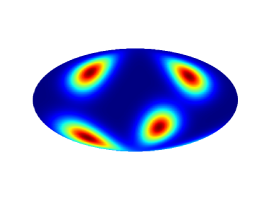
(a) Target

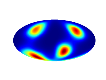
(b) Model

Figure 1: Learned density on $S^{2}$

Manifold	Model	KL[nats]	ESS[%]
$S^{2}$	MS($N_{T}=1$, $K_{m}=12$, $K_{s}=32$)	.05$\pm$.01	90
	MCNF($H=[10,10]$)	.008$\pm$.001	98.4$\pm$.2
$S^{3}$	MS($N_{T}=1$, $K_{m}=32$, $K_{s}=64$)	.14	84
	MCNF($H=[10,10]$)	.013$\pm$.001	97.5$\pm$.2

Table 1: Evaluation of Manifold Continuous Normalizing Flow on Manifold (MCNF) on density matching task. Performance is measured using KL divergence end Effective Sampling Size. $H$ indicates the hidden units in each hidden layer. Results are compared with recursive Möbius-spline flow (MS) (Rezende et al., 2020). $N_{T}$ is the number of stacked transformations for each flow; $K_{m}$ is the number of centres used in Mobius; $K_{s}$ is the number of segments in the spline flow. Error is computed over 3 replicas of each experiment

Appendix B Parameterizing vector fields on manifolds

Given a manifold $M$ we are left with the problem of parameterizing a large enough set of vector fields that allows to express a rich class of distributions on the manifold. When we try to parameterize a large set of function we look at neural networks as a natural solution, however they can only parameterize functions $\mathbb{R}^{n}\to\mathbb{R}^{m}$, and therefore there is no straightforward way to use them. Finding the best way of parameterizing vector fields on manifolds is an interesting problem with no unique solution, how to tackle it will largely depend on how the manifold is defined and what data structure is used to parameterize it in practice. Nevertheless all the objects and methods discussed in the rest of the paper are defined independently from the specific parameterization method chosen. Therefore, if in the future a better way of parameterizing vector fields will emerge, they will still be applicable.

Notwithstanding the above, in this section we will try to give some guidance on how to approach this problem. In the first part we will show how, using generators, it can be reduced to the much easier task of parameterizing functions on manifolds. We will then give some practical advice in the case where the manifold is described using an embedding in $\mathbb{R}^{m}$. Throughout this section, given a function $f:M\to\mathbb{R}^{m}$ we will indicate with $f_{i}:M\to\mathbb{R}$ its $i$-th component, such that $f=(f_{1},\cdots,f_{m})$.

B.1 Local frames and global constraints

We begin by analyzing how we parameterize vector fields in $\mathbb{R}^{n}$, to investigate to what extent we can generalize this procedure. In the euclidean space vector fields are simply functions $f:\mathbb{R}^{n}\to\mathbb{R}^{n}$. In a more geometrical language the function $f$ defines the vector field $X$ in the following way:

$$X=f_{1}\partial{x^{1}}+\cdots+f_{n}\partial{x^{n}}$$ (18)

The converse is also true: for every vector field $X$ there exist a unique continuous function $f:\mathbb{R}^{n}\to\mathbb{R}^{n}$ such that Equation (18) holds. On a generic $n$-dimensional smooth manifold this is only true locally. This means that there exists a open cover $\{U_{i}\}_{i\in\mathcal{I}}$ of $M$, called the trivialization cover, such that $TM$ restricted to each $U_{i}$ is isomorphic to the trivial bundle. This is equivalent to saying that for every set $U_{i}$ there exist $n$ smooth vector fields $E_{1}^{(i)},\cdots,E_{n}^{(i)}\in\Gamma^{\infty}\left(U_{i},TU_{i}\right))$ such that for every smooth vector field $X\in\Gamma^{\infty}\left(M,TM\right)$ there exists a unique smooth function $f:U_{i}\to\mathbb{R}^{n}$ such that:

$$X\bigr{|}_{U_{i}}=f_{1}E_{1}^{(i)}+\cdots+f_{n}E_{n}^{(i)}$$ (19)

We then can call $E_{1}^{(i)},\cdots,E_{n}^{(i)}$ a local frame. A local frame that is defined on an open domain $U=M$ (this means on the entire manifold) is called a global frame. On a manifold there exists plenty of local frames, in fact given a smooth local chart $(U,\{x^{i}\})$ the fields $\partial_{x^{1}},\cdots,\partial_{x_{n}}\in\Gamma^{\infty}\left(U,TU\right)$ form a local frame called coordinate frame. In the special case of $\mathbb{R}^{n}$ its coordinate frame is a global frame. Unfortunately in general not every manifold has a global frame, the simplest example is the sphere $S^{2}$. In the sphere case it is well known that there exists no vector field that is everywhere nonzero, this result goes by the hairy ball theorem. It is then clear that no pair of vector fields $E_{1},E_{2}\in\Gamma^{\infty}\left(M,TM\right)$ can form a global frame, in fact there will always be a point $q\in S^{2}$ such that:

$$\text{span}\left(\left(E_{1}\right)_{q},\left(E_{2}\right)_{q}\right)\leq 1<2=\text{dim}\left(T_{q}M\right)$$ (20)

The manifolds for which a global frame $E_{1},\cdots,E_{n}\in\Gamma^{\infty}\left(M,TM\right)$ exists are called parallelizable manifolds, for this class we can parameterize all smooth vector fields on $M$ in the same way as we did on $\mathbb{R}^{n}$. This means choosing a smooth function $f:M\to\mathbb{R}$ and defining a vector field $X$:

$$X=f_{1}E_{1}+\cdots+f_{n}E_{n}$$ (21)

A manifold is parallelizable iff its tangent bundle is isomorphic to the trivial bundle: $\mathbb{R}^{n}\times M\simeq TM$. A global frame gives an explicit isomorphism:

$$\mathbb{R}^{n}\times M \to TM$$

$$(z,q) \mapsto z_{1}\left(E_{1}\right)_{q}+\cdots+z_{n}\left(E_{n}\right)_{q}$$

An important and large class class of parallelizable manifolds is given by Lie Groups, which are smooth manifold which additionally posses a group structure compatible with the manifold structure. For background on Lie Groups we refer to (Lee, 2013)

B.2 Generators of vector fields

We have seen that for parallelizable manifolds, once we have defined a global frame, we have a bijective correspondence between functions $C^{\infty}(M,\mathbb{R}^{n})$ and smooth vector fields:

$$C^{\infty}(M,\mathbb{R}^{n}) \to\Gamma^{\infty}\left(M,TM\right)$$ (22)

$$f \mapsto f_{1}E_{1}+\cdots+f_{n}E_{n}$$ (23)

For non parallelizable manifolds, we fail to find a global frame because given any $n$ vector fields $\{E_{i}\}_{i=1}^{n}$ there always exist points $q$ where all $\{\left(E_{i}\right)_{q}\}_{i=1}^{n}$ fail to span all $T_{q}M$:

$$\text{span}\left(\{\left(E_{i}\right)_{q}\}_{i=1}^{n}\right)\subsetneq T_{q}M$$

The idea is then to add vector fields to the set $\{\left(E_{i}\right)_{q}\}_{i=1}^{n}$, giving up on the injectivity, until they ”generate” all $\Gamma^{\infty}\left(M,TM\right)$. To make this statement more precise we have to use the language of modules. In fact in general the space of smooth sections of a vector bundle $(E,\pi,M)$ forms a module over the ring $C^{\infty}(M)$ of the smooth functions on $M$.

Definition 4.

A finite set of vector fields $\{X_{i}\}_{i=1}^{m}\subset\Gamma^{\infty}\left(M,TM\right),m\in\mathbb{N}_{>0}$ is a generator of the $C^{\infty}(M)$-module of the smooth vector fields on $M$ if for every vector field $X\in\Gamma^{\infty}\left(M,TM\right)$ there exist $\{f_{i}\}_{i=1}^{m}\subset C^{\infty}(M)$ such that:

$$X=f_{1}X_{1}+\cdots+f_{m}X_{m}$$ (24)

If there exist a generator for for $\Gamma^{\infty}\left(M,TM\right)$ we then say that $\Gamma^{\infty}\left(M,TM\right)$ is finitely generated.

Theorem 3.

Let M be a (second countable) smooth manifold $M$. Then the module of smooth vector fields $\Gamma^{\infty}\left(M,TM\right)$ is finitely generated.

Proof.

Since $M$ is second countable we can apply Lemma 7.1 in (Walschap, 2004) and say that there exist an open trivialization cover $\{U_{i}\}_{i=0}^{n}$, where $n$ is the dimension of $M$. We denote with $E_{1}^{(i)},\cdots,E_{n}^{(i)}$ the local frame relative to the domain $U_{i}\subseteq M$. Now let $\{\psi_{i}\}_{i=0}^{n}$ be a smooth partition of unity subordinate to $\{U_{i}\}_{i=0}^{n}$. We define the global vector fields on $M$:

$$\grave{E}^{(i)}_{j}:=\begin{cases}\psi_{i}\cdot E^{(i)}_{j},&\mbox{on }U_{i}\\ 0&\mbox{on }M\setminus\mbox{supp}\psi_{i}\end{cases}\quad\forall i\in\{0,\cdots,n\}\ \forall j\in\{1,\cdots,n\}$$ (25)

We have that $\{\grave{E}^{(i)}_{j}\}_{\begin{subarray}{c}i=0..n\\ j=1..n\end{subarray}}$ is a generator of $\Gamma^{\infty}\left(M,TM\right)$. To prove this we first define $V_{i}\subseteq M$ as the open set where $\psi_{i}>0$. Since $\sum_{i=1}^{n}\psi_{i}=1$ then also $\{V_{i}\}_{i=0}^{n}$ is an open cover of $M$. Given a global global smooth vector field $X\in\Gamma^{\infty}\left(M,TM\right)$, for each $V_{i}$ there exist $f^{(i)}_{1},\cdots,f^{(i)}_{n}\in C^{\infty}(V_{i})$ such that:

$$X=_{V_{i}}\sum_{j=1}^{n}f^{(i)}_{j}\grave{E}^{(i)}_{j}\quad\forall i\in\{1,\cdots,n\}$$ (26)

Now let $\{h_{i}\}_{i=0}^{n}$ a smooth partition of unity subordinated to $\{V_{i}\}_{i=0}^{n}$. We use it to define the global smooth functions:

$$\grave{f}^{(i)}_{j}:=\begin{cases}h_{i}\cdot f^{(i)}_{j},&\mbox{on }V_{i}\\ 0&\mbox{on }M\setminus\mbox{supp}h_{i}\end{cases}\quad\forall i\in\{0,\cdots,n\}\ \forall j\in\{1,\cdots,n\}$$ (27)

Combining equation (26) and with the fact that $\sum_{i=1}^{n}h_{i}=1$ we have:

$$X=\sum_{i=0}^{n}\sum_{j=1}^{n}\grave{f}^{(i)}_{j}\grave{E}^{(i)}_{j}$$ (28)

∎

From this Theorem and the definition of generator we can extract a methodology to parameterize all vector fields on smooth manifolds:

1. choose a suitable set of generators $\{X_{i}\}_{i=1}^{m}$

2. find a way of parameterizing functions $f_{i}:M\to\mathbb{R}$

3. model a generic vector field $X$ as a linear combination:

   $$X=f_{1}X_{1}+\cdots+f_{m}X_{m}$$ (29)

The above proof also tells us that a simple and general recipe to obtain a generator is to take a collection of local frames and multiply them by a smooth partition of unity. The efficiency of this framework is given by the cardinality of the generator: lower cardinality requires parameterization of less functions. The proof gives us an initial upper bound on the lowest cardinality of the set of generators we can achieve for a generic manifold: $n^{2}+n$ where $n$ is the dimension of the manifold. We will see that for Riemannian manifolds, using the Whitney embedding theorem this number can be further reduced to $2n+1$.
However the cardinality of the generator is not the only factor to consider when choosing a good generating set. In fact combining equation (29) with the properties of Lie derivative we obtain:

$$\textnormal{div}{\left(X\right)}=\sum_{i=1}^{m}X_{i}(f_{i})+f_{i}\textnormal{div}{\left(X_{i}\right)}$$ (30)

If we can find a set of generators with known divergence, or for which we can (pre-)compute the divergence, this greatly simplifies the divergence computation.

B.2.1 Time dependent vector fields

When parameterizing time dependent vector fields vector fields we have to model a vector field $X_{t}$ for all $t\in\mathbb{R}$. Using generators we can easily accomplish this by parametrizing a function $f:\mathbb{R}\times M\to\mathbb{R}^{m}$ and defining

$$X_{t}:=f_{1}(t,\cdot)X_{1}+\cdots+f_{m}(t,\cdot)X_{m}$$ (31)

B.3 Embedded submanifolds of $\mathbb{R}^{m}$

Definition 5.

Let $N$, $M$ smooth manifolds and $F:M\to N$ a smooth function between them. Given $X\in\Gamma^{\infty}\left(M,TM\right)$ and $Y\in\Gamma^{\infty}\left(N,TN\right)$ smooth vector fields respectively on $M$ and $N$, we say that they are F-related if

$$dF_{p}\left(X_{p}\right)=Y_{F(p)}\quad\forall p\in M$$ (32)

A general way to work in practice with manifolds is using embedded submanifolds of $\mathbb{R}^{m}$. An embedding for a manifold $M$ is a continuous injective function $\iota:M\hookrightarrow\mathbb{R}^{m}$ such that $\iota:M\to\iota(M)$ is a homeomorphism. The embedding is smooth if $\iota$ is smooth and $M$ is diffeomorphic to its image. In this case $\iota(M)$ is a smooth submanifold of $\mathbb{R}^{m}$. For all practical purposes we can directly identify $M$ as a submanifold of $\mathbb{R}^{m}$, the function $\iota:M\hookrightarrow\mathbb{R}^{m}$ then simply denotes the inclusion. Through this identification we can then consider the tangent space $T_{q}M,\ q\in M$ as a vector subspace of $T_{q}\mathbb{R}^{m}$. An embedding is said proper if $\iota(M)$ is a closed set in $\mathbb{R}^{m}$.

Theorem 4 (Whitney Embedding Theorem, 6.15 in (Lee, 2013)).

Every smooth $n$-dimensional manifold admits a proper smooth embedding in $\mathbb{R}^{2n+1}$

The Whitney embedding theorem tells us that parameterizing manifolds as submanifolds of the Euclidean space gives us a general methodology to work with manifolds. Developing algorithms that assume that the manifold is given as an embedded submanifold of $\mathbb{R}^{m}$ is therefore of outstanding importance.

For embedded submanifolds parameterizing functions is extremely easy, and can be simply done via restriction: given a smooth function $f:\mathbb{R}^{m}\to\mathbb{R}$, $f\circ\iota$ then defines a smooth function from $M$ to $\mathbb{R}$.

Unfortunately for vector fields it is not as easy as for functions, in fact in general given a vector field $X\in C(\mathbb{R}^{m},T\mathbb{R}^{m})$ this does not restrict in general to a vector field on a submanifold $M\subseteq\mathbb{R}^{m}$, as in general given $q\in M$ we have $X_{q}\not\in T_{q}M\subseteq T\mathbb{R}_{q}^{m}$. In order for $X$ to restrict to a vector field on a submanifold $M$ we need for $X$ to be tangent to the submanifold :

$$X_{q}\in T_{q}M\subseteq T_{q}\mathbb{R}^{m}\quad\forall q\in M$$ (33)

A tangent vector field then defines a vector field on the submanifold:

Lemma 1.

Let $M$ be a smoothly embedded submanifold of $\mathbb{R}^{m}$, and let $\iota:M\hookrightarrow\mathbb{R}^{m}$ denote the inclusion map. If a smooth vector field $Y\in\Gamma^{\infty}\left(\mathbb{R}^{m},T\mathbb{R}^{m}\right)$ is tangent to $M$ there is a unique smooth vector field on $M$, denoted by $Y|_{M}$ , that is $\iota$-related to $Y$. Conversely a vector field $\overline{Y}\in\Gamma^{\infty}\left(\mathbb{R}^{m},T\mathbb{R}^{m}\right)$ that is $\iota$-related to $Y$ is tangent to $M$

Proof.

See proof of Proposition 8.23 in (Lee, 2013) ∎

More importantly we can parameterize all vector fields on an embedded submanifold using tangent vector fields:

Prop 1.

Let $M$ be a properly embedded submanifold of $\mathbb{R}^{m}$, and let $\iota:M\hookrightarrow\mathbb{R}^{m}$ denote the inclusion map. For any smooth vector field $X\in\Gamma^{\infty}\left(M,TM\right)$ there exist a smooth vector field $\overline{X}\in\Gamma^{\infty}\left(\mathbb{R}^{m},T\mathbb{R}^{m}\right)$ tangent to $M$ such that:

$$\overline{X}|_{M}=X$$ (34)

We call $\overline{X}$ an extension of $X$.

Proof.

Let $U\subseteq\mathbb{R}^{m}$ be a tubular neighborhood of $M$, then by Proposition 6.25 of (Lee, 2013) there exist a smooth map $r:U\to M$ that is both a retraction and a smooth submersion. Then since $r$ is a submersion there exist a vector field $\overline{X}\in\Gamma^{\infty}\left(U,TU\right)$ that is $r$-related to $X$ . This means $dr_{z}\overline{X}_{z}=X_{r(z)}\forall z\in\mathbb{R}^{m}$. Since $r$ is a retraction

$$d\iota_{q}\circ dr_{q}=Id_{T_{q}\mathbb{R}^{m}}\ \Rightarrow\ \left(d\iota_{q}\circ dr_{q}\right)\overline{X}_{q}=\overline{X}_{q}\Rightarrow\ d\iota_{q}X_{q}=\overline{X}_{q}\ \forall q\in M,$$ (35)

$\overline{X}$ is $\iota$-related to $X$ and therefore tangent to $M$ and such that $\overline{X}|_{M}=X$. Then $\overline{X}$ can be used to define a tangent vector field on all $\mathbb{R}^{m}$ using a smooth partition of unity subordinate to the open cover $\{\mathbb{R}^{m}\setminus M,U\}$. ∎

From the proof of the theorem it’s clear that the extension of $X$ is not unique. Our objective is then finding a way to parameterize all vector fields tangent to a submanifold. We first observe that given smooth vector fields $X,Y\in\Gamma^{\infty}\left(\mathbb{R}^{m},T\mathbb{R}^{m}\right)$ tangent to $M$ and smooth functions $f,g\in C^{\infty}(\mathbb{R}^{m})$ then $fX+gY$ is tangent to $M$. This means that the set of all smooth vector fields tangent to $M$ is a submodule of the module of smooth vector fields on $\mathbb{R}^{m}$. Following the framework outlined in Section B.1 we then need to find $l$ tangent vector fields $\overline{X}_{1},\cdots,\overline{X}_{l}$ such that $\overline{X}_{1}|_{M},\cdots,\overline{X}_{l}|_{M}$ generates all $\Gamma^{\infty}\left(M,TM\right)$.

B.3.1 Embedded Riemannian Submanifolds

If our embedded submanifold manifold is equipped with a Riemannian metric, the gradient of the embedding gives us a set of generators for the tangent bundle. We first prove the following lemma

Lemma 2.

Let $M$ be a embedded submanifold of $N$, and let $\iota:M\hookrightarrow N$ denote the inclusion map. Then

$$\iota^{*}:\iota^{*}T^{*}N \to T^{*}M$$ (36)

$$\beta_{\iota(q)} \mapsto\iota^{*}\beta_{\iota(q)}:\quad v\mapsto\beta_{\iota(q)}(dv_{q})\quad\forall q\in M,\ \forall\beta\in T^{*}_{\iota(q)}N,\ \forall v_{q}\in T_{q}M$$ (37)

is a surjective vector bundle homomorphism, where by $\iota^{*}T^{*}N$ we denote the pullback bundle $\iota^{*}T^{*}N=\{(q,\beta)\in M\times T^{*}N|\pi(\beta)=\iota(q)\}$

Proof.

Fix $q\in M$.Let $n$ be the dimensionality of $M$ and $m$ the dimensionality of $N$. We need to prove that $\iota^{*}:T^{*}_{\iota(q)}N\to T^{*}_{q}M$ is surjective. Let $e_{1},\cdots,e_{n}$ a basis for $T_{q}M$ and $\eta_{1},\cdots,\eta_{n}$ its dual basis. By the linearity of $\iota^{*}$ it’s then sufficient to prove that there exists $\beta_{1},\cdots,\beta_{n}\in T^{*}_{\iota(q)}N$ such that for all $i\in\{1,\cdots,n\}$:

$$\iota^{*}\beta_{i}=\eta_{i}$$ (38)

To see this, consider the set $\{d(\eta_{1})_{q},\cdots,d(\eta_{n})_{q}\}\subset T_{\iota(q)}N$. Since $\iota$ is an embedding, $d\iota$ is injective. Therefore the vectors are linearly independent. We can then complete them to a basis $v_{1}:=d(\eta_{1})_{q},\cdots,w_{n}:=d(\eta_{n})_{q},w_{n+1},\cdots w_{m}$ of $T_{\iota(q)}N$. Let $\beta_{1},\cdots,\beta_{m}\in T^{*}_{\iota(q)}N$ the dual basis. We then have:

$$\iota^{*}\beta_{i}(e_{j})=\beta_{i}\left(d\left(\eta_{j}\right)_{q}\right)=\beta_{i}\left(w_{j}\right)=\delta_{ij}=\eta_{i}\left(e_{j}\right)\quad\forall i,j\in\{1,\cdots,n\}$$ (39)

Thus $\beta_{i}$ satisfies Equation (38) $\forall i\in\{1,\cdots,n\}$ ∎

Theorem 5.

Let $(M,g)$ be a embedded submanifold of $\mathbb{R}^{m}$, and let $z:M\hookrightarrow\mathbb{R}^{m}$ denote the inclusion map. Then $\{\nabla z_{i}\}_{i=1}^{m}$ is a set of generators for smooth vector fields $\Gamma^{\infty}\left(M,TM\right)$. Where $\nabla$ denotes the Riemannian gradient with respect to the metric $g$.

Proof.

Consider the differential forms $\{dz_{i}\}_{i=1}^{m}\subset\Gamma^{\infty}\left(M,T^{*}M\right)$. Using Lemma 2 we have that $\text{span}\left(\{dz_{i}(q)\}_{i=1}^{m}\right)=T^{*}_{q}M$, which means that at every point they span the cotangent space at the point. Using the musical isomorphism, this implies that the riemannian gradients $\nabla z_{i}$ span the tangent space at every point: $\text{span}\left(\{\nabla z_{i}(q)\}_{i=1}^{m}\right)=T_{q}M$. From this we can conclude that $\{\nabla z_{i}\}$ is a generator for $\Gamma^{\infty}\left(M,TM\right)$. To see this consider the open sets $U_{I}:=\{q\in M|\{\nabla z_{i}(q)\}_{i\in I}\quad\text{are linearly independent}\}$ where $I\subset\{1,\cdots,m\}$ is any subset of indices of cardinality $n$. To see that these sets are open, observe that in a local coordinate chart $(U,(x_{i}))$ we can write $\nabla z_{i_{k}}|_{U}=\sum_{j=1}^{n}a^{I}_{i,j}\partial_{x_{j}}\forall i\in{1,\cdots,M}$. In local coordinates the linear independence of $\{\nabla z_{i}\}_{i\in I}$, is equivalent to $\text{det}(A(x))\neq 0$. Where if $I={i_{1},\cdots,i_{n}}$ $A(x)$ is defined as $A(x)_{jk}=a^{I}_{i_{k},j}$. From the definition of $U_{I}$ it descends that the family $\{(U_{I}|I\subset\{1,\cdots,m\},\ \#(I)=n,\ U_{I}\text{is not empty}\}$ forms a open trivialization. We can then conclude proceeding as in the proof of Theorem 3 ∎

In general, given a function $f\in C^{\infty}(M)$ on a Riemannian manifold, its Laplacian is defined as the divergence of its Riemannian gradient:

$$\Delta f:=\textnormal{div}{\left(\nabla f\right)}$$ (40)

Then the divergence of the fields defined in Theorem 3 is given by the Laplacian of the functions $z_{i}:M\to\mathbb{R}$.

B.3.2 Isometrically embedded Submanifolds

If the manifold $M$ is isometrically embedded in $\mathbb{R}^{n}$. Then $\nabla z_{i}$ is simply given by the orthogonal projection of the constant coordinate field $e_{i}=\partial_{x_{i}}$ from $T\mathbb{R}^{m}$ to $TM$. In this case the Laplacian of the functions $z_{i}:M\to\mathbb{R}$ is given by the mean curvature (Chen & Verstraelen (2013), Proposition 2.3):

$$\Delta z=nH=\text{tr}\ \mathrm{I}\!\mathrm{I},$$ (41)

where $H$ is the mean curvature and $\mathrm{I}\!\mathrm{I}$ is the second fundamental form.

For the hypersphere $S^{n}$, the projection expression is particularly simple. This gives us $n+1$ vector fields $\{\overline{\nabla z_{i}}\}_{i=1}^{n+1}\subset\Gamma^{\infty}\left(\mathbb{R}^{n+1},T\mathbb{R}^{n+1}\right)$ tangent to $S^{n}$ such that their restriction to $M$ forms a generator for $\Gamma^{\infty}\left(S^{n},TS^{n}\right)$.

$$\overline{\nabla z_{i}}=e_{i}-\langle z,e_{i}\rangle z\quad\forall i\in\{1,\cdots,n+1\}$$ (42)

$$\Delta z=-nz$$ (43)

References

- Agrachev et al. (2019) Agrachev, A., Barilari, D., and Boscain, U. A comprehensive introduction to sub-riemannian geometry, 2019.
- Agrachev & Sachkov (2013) Agrachev, A. A. and Sachkov, Y. Control theory from the geometric viewpoint, volume 87. Springer Science & Business Media, 2013.
- Bose et al. (2020) Bose, A. J., Smofsky, A., Liao, R., Panangaden, P., and Hamilton, W. L. Latent variable modelling with hyperbolic normalizing flows. arXiv preprint arXiv:2002.06336, 2020.
- Bullo & Lewis (2004) Bullo, F. and Lewis, A. Supplementary chapters for ”geometric control of mechanical systems”. 06 2004.
- Chen & Verstraelen (2013) Chen, B.-Y. and Verstraelen, L. Laplace transformations of submanifolds, 2013.
- Chen et al. (2018) Chen, R. T. Q., Rubanova, Y., Bettencourt, J., and Duvenaud, D. K. Neural ordinary differential equations. In Bengio, S., Wallach, H., Larochelle, H., Grauman, K., Cesa-Bianchi, N., and Garnett, R. (eds.), Advances in Neural Information Processing Systems 31, pp. 6571–6583. Curran Associates, Inc., 2018.
- Da Silva (2001) Da Silva, A. C. Lectures on symplectic geometry, volume 3575. Springer, 2001.
- Davidson et al. (2018) Davidson, T. R., Falorsi, L., De Cao, N., Kipf, T., and Tomczak, J. M. Hyperspherical variational auto-encoders. 34th Conference on Uncertainty in Artificial Intelligence (UAI-18), 2018.
- Falorsi et al. (2018) Falorsi, L., de Haan, P., Davidson, T. R., De Cao, N., Weiler, M., Forré, P., and Cohen, T. S. Explorations in homeomorphic variational auto-encoding. ICML workshop on Theoretical Foundations and Applications of Deep Generative Models, 2018.
- Falorsi et al. (2019) Falorsi, L., de Haan, P., Davidson, T. R., and Forré, P. Reparameterizing distributions on lie groups. AISTATS, 2019.
- Finlay et al. (2020) Finlay, C., Jacobsen, J.-H., Nurbekyan, L., and Oberman, A. M. How to train your neural ode: the world of jacobian and kinetic regularization, 2020.
- Gemici et al. (2016) Gemici, M. C., Rezende, D., and Mohamed, S. Normalizing flows on riemannian manifolds. arXiv preprint arXiv:1611.02304, 2016.
- Grathwohl et al. (2019) Grathwohl, W., Chen, R. T. Q., Bettencourt, J., and Duvenaud, D. Scalable reversible generative models with free-form continuous dynamics. In International Conference on Learning Representations, 2019.
- Haber & Ruthotto (2017) Haber, E. and Ruthotto, L. Stable architectures for deep neural networks. Inverse Problems, 34(1):014004, 2017.
- Hairer (2011) Hairer, E. Solving differential equations on manifolds. 2011.
- Khalil et al. (2017) Khalil, S. A., Basheer, M. A., and Abdelhaleem, T. A. Types of derivatives: Concepts and applications (ii). Journal of Mathematics Research, 9(1), 2017.
- Kingma & Ba (2015) Kingma, D. P. and Ba, J. Adam: A method for stochastic optimization. International Conference on Learning Representations, 2015.
- Lee (2013) Lee, J. M. Smooth manifolds. In Introduction to Smooth Manifolds. Springer, 2013.
- Nagano et al. (2019) Nagano, Y., Yamaguchi, S., Fujita, Y., and Koyama, M. A wrapped normal distribution on hyperbolic space for gradient-based learning. In International Conference on Machine Learning, pp. 4693–4702, 2019.
- Papamakarios et al. (2019) Papamakarios, G., Nalisnick, E., Rezende, D. J., Mohamed, S., and Lakshminarayanan, B. Normalizing flows for probabilistic modeling and inference. stat, 1050:5, 2019.
- Pontryagin et al. (1962) Pontryagin, L. S., Mishchenko, E., Boltyanskii, V., and Gamkrelidze, R. The mathematical theory of optimal processes. Wiley, 1962.
- Pérez Rey et al. (2019) Pérez Rey, L. A., Menkovski, V., and Portegies, J. W. Diffusion variational autoencoders. arXiv, 2019.
- Rezende & Mohamed (2015) Rezende, D. and Mohamed, S. Variational inference with normalizing flows. In International Conference on Machine Learning, pp. 1530–1538, 2015.
- Rezende et al. (2020) Rezende, D. J., Papamakarios, G., Racanière, S., Albergo, M. S., Kanwar, G., Shanahan, P. E., and Cranmer, K. Normalizing flows on tori and spheres. arXiv preprint arXiv:2002.02428, 2020.
- Walschap (2004) Walschap, G. Metric Structures in Differential Geometry. Graduate Texts in Mathematics. Springer, softcover reprint of hardcover 1st ed. 2004 edition, 2004. ISBN 1441919139,9781441919137.