Universal collective Larmor-Silin mode emerging in magnetized correlated Dirac fermions

Abstract

Employing large-scale quantum Monte Carlo simulations, we find in magnetized interacting Dirac fermion model, there emerges a new and universal collective Larmor-Silin spin wave mode in the transverse dynamical spin susceptibility. Such mode purely originates from the interaction among Dirac fermions and distinguishes itself from the usual particle-hole continuum with finite lifetime and clear dispersion, both at small and large momenta in a large portion of the Brillouin zone. Our unbiased numerical results offer the dynamic signature of this new collective excitations in interacting Dirac fermion systems, and provide experimental guidance for inelastic neutron scattering, electron spin resonance and other spectroscopic approaches in the investigation of such universal collective modes in quantum Moiré materials, topological insulators and quantum spin liquid materials under magnetic field, with quintessential interaction nature beyond the commonly assumed noninteracting Dirac fermion or spinon approximations.

Introduction.— Collective excitations offer the fingerprint of quantum many-body systems, given them the spin wave in the magnetically ordered systems [1, 2, 3, 4, 5], the roton mode in the superfulid [6, 7, 8, 9, 10, 11], excitons and magnetorotons in the quantum moiré materials, integer and fractional quantum (anomalous) Hall systems [12, 13, 14, 15, 16, 17, 18] and many others. And it is oftentimes the case that the identification of new collective excitations provide the decisive understanding of the physical nature of the corresponding quantum many-body ground states.

The situation becomes subtle in the highly entangled quantum matter, where the collective excitations are harder to identify in an unbiased manner. For example, in the study of quantum spin liquid (QSL) states, it is well known that the identification from specific experimental signature the unique aspect of a QSL state is difficult, as there usual exist multiple explanations for the same experimental data [19, 20, 21, 19]. One crucial property of QSL is the emergence of fractionalized excitations, such as spinons (carry a spin of 1/2 but charge-neutral), which are elementary quasiparticles carrying topological characteristics and interacting with an emergent gauge field [22, 23, 24, 25, 26, 27, 28, 29, 30]. In Dirac QSLs, spinons can exhibit a conical dispersion, resembling Dirac cones in the electronic band structures of graphene, topological insulators and many 2D materials [31, 32, 33, 34].

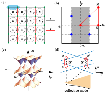
Figure 1: (a) Schematic plot of the Hamiltonian Eq. (1), the $\pi$-flux model on the square lattice. The black lines stand for hopping strength of fermion with $t_{ij}=+1$, while the red lines are $t_{ij}=-1$. Such arrangement ensures that the flux threaded each plaquette is $\pi$, giving Dirac cones at zero magnetic field. The blue ellipse enclosing two lattice sites is the unit cell. (b) BZ of the original square lattice (white) and the folded BZ (grey) with blue ellipse as unit cell. The path denoted by the red line connects high symmetry momenta $\Gamma(0,0)$, $X(\pi,0)$ and $M(\pi,\pi)$ in BZ for the original square lattice. (c) The splitted Fermi surface of $\pi$-flux model under external magnetic field in $z$ direction. (d) Schematic plot that depicts the origin of the collective mode. The coherent excitation of spin flip $S^{+}$ and $S^{-}$ in the model gives rise to the collective mode.

While detecting a single spinon excitation is challenging, their collective excitations – the two spinon excitations with a total spin quantum number $S$ = 1 can lead to a spin continuum spectrum that can be detected through inelastic neutron scattering techniques. Such characteristic collective conitnum spectra have been reported in materials such as the kagome lattice antiferromagnets ZnCu₃(OH)₆Cl₂ [35], Cu₃Zn(OH)₆FBr [36] and YCu₃(OH)₆Br₂[Br_1-x(OH)_x] [37, 38, 39, 40, 41].

However, in these studies of QSL, one often assumes the fractionalized spinons are nearly free particles and computed their collective modes (continuum spectrum) under such assumption, i.e., the convolution of two independent spectra of single spinon [42, 43, 44]. But in reality, it is obvious that the spinons experience strong interactions, mediated by the fluctuations of gauge fields [45, 46, 27, 28, 47, 48, 26], and such assumption is oversimplified and often leads to contradictions or controversies, when trying to interpret the experimental data and make predictions [49, 50].

Therefore, one needs to either solve the interacting problem completely, usually via unbiased numerical approches [26, 27, 28, 47, 29, 25, 30], or find new signatures which are robust beyond the nearly-free approximations, even with interaction effect included. But none of these two strategies are simple and the progresses are usually made in a case by case manner. Recently, an interesting proposal of the latter strategy coming to our attention. In the Refs. [51, 52, 53], the authors propose a new collective ”spinon spin wave” mode to emerge in the transverse dynamical spin susceptibility – different from the usual spin continuum spectra – in the 2D Dirac QSL subjected to an applied Zeeman field, and tested their proposal rigoroulsy in 1D Heisenberg chain via DMRG simulations and in 2D magnetized graphene in perturbative analysis.

In fact, the suggested collective modes date back to early investigations of the spin response of paramagnetic metals subjected to the external magnetic field, denoted as the transverse Larmor-Silin spin wave [54, 55], in the form of collective spin oscillations in itinerant interacting fermion systems [56, 57, 58, 59]. Phenomenologically, such Larmor-Silin spin wave is the transverse collective spin mode below the particle-hole continuum of, say, a single-band conductors with parabolic electron dispersion. This downward dispersing collective mode is the precession of the total magnetic moment originating from the Zeeman frequency at zero wave vector (as schematically shown in Fig. 1 (d)) and of purely interacting nature. The ”spinon spin wave” in Refs. [51, 52, 53], can therefore be viewed as the modern version of the Larmor-Silin spin wave, in the context of magnetized graphene and 2D Dirac QSL.

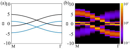
Figure 2: (a) Free fermion dispersion under magnetic field $B=3.4$. Because of polarization, the spin degeneracy is lifted and four bands are visible. (b) Single particle spectra $A(k,\omega)$ from QMC+SAC with parameter $U=2,B=3.4$ on a $16\times 16$ lattice. The gap at $(\frac{\pi}{2},\frac{\pi}{2})$ is around 2.34, corresponding to an effective magnetic field $B_{\text{eff}}=4.68$ in Eq. (2).

Until now, the unbiased 2D lattice model verification of the ”spinon spin wave”, i.e., to complete both strategies of unbiased numerical calculation of the purely interaction-generated collective mode, has not been carried out. This is due, of course, to both the lack of proper lattice model design and the numerical difficulties in solving the interacting model accurately. In this work, we finally achieve both goals successfully, by employing large-scale quantum Monte Carlo (QMC) simulations, substantiated with random phase approximation (RPA) analysis, to find in a concrete 2D magnetized interacting Dirac fermion lattice model, there emerges the universal collective Larmor-Silin spin wave mode in the transverse dynamical spin susceptibility. Beyond the perturbative proposals [52, 53], we find in the 2D lattice model, the Larmor-Silin spin wave not only splits off from the usual ”two-spinon continuum” at small momenta, but also universally appears inside and at the bottom of the continuum at large momenta, with richer renormalization effects and magnetic field dependence. Our unbiased numerical results offer the dynamic signature of this new collective mode in interacting Dirac fermion systems, and provide experimental guidance in its detection in quantum Moiré materials, topological insulator and Dirac spin liquid materials, under magnetic field.

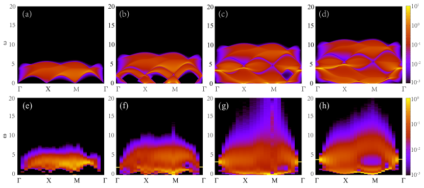
Figure 3: Transverse magnetic spectra $S_{\pm}(\mathbf{q},\omega)$ under $z$ direction magnetic field at $U=2$. Panels (a), (b), (c) and (d) are the spectra from RPA spin susceptibilities $\chi_{\pm}(\mathbf{q},\omega)$ with $B=0,2,3.4,4$. Panels (e), (f), (g) and (h) are the spectra from QMC+SAC results with $B=0,2,3.4,4$. As magnetic field $B$ increases, the universal collective transverse mode emerges, not only close to $\Gamma$ but also at higher momenta and inside the spin continuum. The RPA and QMC spin spectra are consistent with each other.

Model and Method.— Our model has the following Hamiltonian on a 2D square lattice,

$$H =H_{0}+H_{U}+H_{B},$$ (1)

$$H_{0} =-\sum_{\langle i,j\rangle,\sigma}(t_{ij}c^{\dagger}_{i,\sigma}c_{j,\sigma}+h.c.)$$

$$H_{U} =\frac{U}{2}\sum_{i}(n_{i\uparrow}+n_{i\downarrow}-1)^{2}$$

$$H_{B} =-B\sum_{i}\frac{1}{2}(c^{\dagger}_{i,\uparrow}c_{i,\uparrow}-c^{\dagger}_{i,\downarrow}c_{i,\downarrow})$$

as shown in Fig. 1 (a), the hopping strength $t_{ij}$ on black (red) bonds are $+1$ $(-1)$, ensuring the flux threaded each plaquette is equal to $\pi$. $\sigma=\uparrow,\downarrow$ denotes spin flavors. The blue ellipse denotes the unit cell, which contains two sites. The Brillouin zone (BZ), shown in Fig. 1(b), is folded with $k_{x}\in[-\pi/2,\pi/2)$ and $k_{y}\in[-\pi,\pi)$. The free dispersion has two independent Dirac points denoted by the blue solid points. Near the Dirac points, the dispersion has good linear form. The interaction in the model is the on-site Hubbard repulsion with strength $U$. The $S^{z}_{i}=\frac{1}{2}(c^{\dagger}_{i,\uparrow}c_{i,\uparrow}-c^{\dagger}_{i,\downarrow}c_{i,\downarrow})$ of fermion is coupled to an external magnetic field in $z$ direction with strength $B$. The effect of magnetic field $B$ can be interpreted as that the spin up and spin down fermion have chemical potential with opposite sign.

Without external magnetic field, the $\pi$-flux Hubbard model with spin $1/2$ fermion has a Dirac semi-metal to antiferromagnetic Néel state quantum phase transition at finite $U_{c}$, with the latter state spontaneously breaks $SU(2)$ spin rotational symmetry [60, 61, 62, 63, 64]. With plaquette interactions, extended beyond on-site, it is also found via large-scale QMC simulation that the model can host a $U(1)$ Dirac QSL phase, via nontrivial deconfined quantum critical point [65, 66, 67, 68]. It is fair to assert that the $\pi$-flux Dirac fermion model can be used to describe the spinon dispersion of a $U(1)$ Dirac QSL [69]. Therefore, the spin spectra of our model can help to understand that of $U(1)$ Dirac QSL under magnetic field. Admittedly, the present model does not have the dynamical $U(1)$ gauge field and we shall leave it for future work.

RPA Analysis.— Firstly we investigate the model Eq. (1) with random phase approximation (RPA) following the work [52]. The detailed calculation scheme is given in the Sec. I of Supplemental Material (SM) [70]. We define magnetization as $M=\frac{1}{2}(\frac{N_{\uparrow}-N_{\downarrow}}{N_{\uparrow}+N_{\downarrow}})$, where $N_{\uparrow}$ ($N_{\downarrow}$) is the particle number of up (down) fermion. The system is at half-filling, $N_{\text{tot}}=N_{\uparrow}+N_{\downarrow}=L^{2}/2$, where $L$ is the linear system size. The contribution to the Green’s function from Hubbard interaction $U$ is approximately treated as Hartree energy shift. The fermion dispersions are shifted by $-UM$ for up spin and $UM$ for down spin. In practice, we find it more appropriate to use renormalized interaction strength $U_{\text{eff}}$ in RPA calculation. As shown in Fig. 2, in QMC we can obtain the effective magnetic field $B_{\text{eff}}$ which is $2$ times the gap at Dirac point $(\pi/2,\pi/2)$ from single particle spectra $A(\mathbf{k},\omega)$ . $B_{\text{eff}}$ is then related to $U_{\text{eff}}$ by

$$B_{\text{eff}}=B+U_{\text{eff}}M.$$ (2)

The renormalized interaction strength $U_{\text{eff}}$ is then calculated as $U_{\text{eff}}=\frac{B_{\text{eff}}-B}{M}$. Consider the effective Hamiltonian, $\epsilon_{a,\sigma}(k)=(-1)^{a}\sqrt{\cos^{2}\mathbf{k}_{x}+\cos^{2}\mathbf{k}_{y}}-\alpha(\sigma)B_{\text{eff}}/2$, where $a\in[1,2]$ denotes the band index and $\alpha=+1(-1)$ for $\uparrow(\downarrow)$ spin . We then calculate the bare transverse spin susceptibility $\chi^{0}_{\pm}$ with standard fermion loop diagram. The RPA spin susceptibility $\chi_{\pm}$ is obtained by resummation of particle-hole ladder diagrams with $\chi^{0}_{\pm}$ as bare susceptibility [71]

$$\chi_{\pm}(\mathbf{q},i\omega_{n})=\frac{\chi^{0}_{\pm}(\mathbf{q},i\omega_{n})}{1+U_{\text{eff}}\chi^{0}_{\pm}(\mathbf{q},i\omega_{n})}.$$ (3)

After analytic continuation $i\omega_{n}\rightarrow\omega+i0^{+}$, the spin spectra $S_{\pm}(\mathbf{q},\omega)=-\text{Im}\chi_{\pm}(\mathbf{q},\omega)$, which will be directly compared with QMC results. The existence of the universal collective mode is already manifested at RPA spin susceptibility [71, 52] and the condition for its emergence is discussed in details in SM [70].

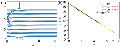
Figure 4: (a) Spectra $S_{\pm}(\mathbf{q},\omega)$ from QMC+SAC at $U=2,B=4$. The red lines highlight the high symmetry momentum points in BZ. (b) Logscale plot of imaginary-time spin correlation function $S_{\pm}(\mathbf{\Gamma},\tau)$ from QMC simulation with $B=4$ and varying $U$.

QMC Simulation and Results.— We further investigate the model with finite-temperature determinant quantum Monte Carlo (DQMC) simulations [72, 73]. The model in Eq. (1) is particle-hole symmetric and thus sign-problem free [74, 75]. We use the Hubbard-Stratonovich (HS) decomposition to decouple the interaction into density channel and perform the simulations on a $16\times 16$ square lattice (at the inverse temperature $\beta t=L$ and $t=1$ as the energy unit) at $U=2$ with varying external magnetic field $B$. The external magnetic field $B$ enters the DQMC as chemical potential term for canonical ensemble simulations, with opposite sign for opposite spin flavor, and still renders the simulation sign-problem free. At large $U$ and finite $B$, the system will break the $U(1)$ spin rotational symmetry and enter a AFXY insulator phase [60], but we purposely stay in the paramagnetic phase to investigate the transverse Larmor-Silin spin wave mode. The details of DQMC implementation is given in Sec. II of SM [70].

Firstly we calculate the imaginary time Green’s function $G_{\sigma}(\mathbf{k},\tau)$ and use the stochastic analytic continuation (SAC) [76, 77, 78, 1, 25, 26, 28, 48] to obtain the real frequency single particle spectral function $A(\mathbf{k},\omega)$. The result of $A(\mathbf{k},\omega)$ is shown in Fig. 2 (b) comparing with dispersion of free fermion under the same external magnetic field in Fig. 2 (a). As shown in the Figure, the degeneracy of energy bands is lifted by the external magnetic field $B$, giving rise to pocket like Fermi surface showed in Fig. 1(c). In our lattice simulation with $L=16,\beta=16,U=2,B=3.4$, the QMC single particle spectra shows that the magnetized system is still in metallic state, and the amount of energy shift is larger compared to the free system with $U=0,B=3.4$, which can be attributed to the renormalization effect of the Hubbard interaction. This further confirms the usage of effective Hubbard $U_{\text{eff}}$ as Hartree energy shift in RPA calculation.

Next we focus on the spin spectra of the magnetized Dirac fermions. We compute the dynamical transverse spin correlation function

$$S_{\pm}(\mathbf{q},\tau)=\frac{1}{L^{4}}\sum_{i,j}\left<S^{+}_{i}(\tau)S^{-}_{j}(0)\right>e^{-i(r_{i}-r_{j})\cdot\mathbf{q}}.$$ (4)

where $S^{+}_{i}=c^{\dagger}_{i,\uparrow}c_{i,\downarrow}$ and $S^{-}_{i}=c^{\dagger}_{i,\downarrow}c_{i,\uparrow}$. The same as $A(\mathbf{k},\omega)$, we can obtain the spin spectra $S_{\pm}(\mathbf{q},\omega)$ from $S_{\pm}(\mathbf{q},\tau)$ utilizing SAC, whose details are given in Sec. II of SM [70].

The results are depicted in Fig. 3. The upper panels are RPA spin spectra $S_{\pm}(\mathbf{q},\omega)$, while the lower panels are QMC results, with the parameters $U=2$, $L=\beta=16$. The RPA calculations are at zero temperature with $50\times 100$ momentum grid (considering the unit cell, the BZ is folded with $k_{x}\in[-\pi/2,\pi/2)$ and $k_{y}\in[-\pi,\pi)$). The effective $U_{\text{eff}}$ in the RPA panels are determined according to Eq. (2) with the help of single particle spectra $A(\mathbf{k},\omega)$. For $B=2,3.4,4$, effective $U_{\text{eff}}=2.86,1.69,1.67$ respectively. Without magnetic field at $U=2$, the manetization $\left<M\right>=0$ in QMC, thus use $U_{\text{eff}}=U=2$ in RPA.

In Fig. 3, we increase the magnetic field from left to right. At $B=0$, we have the well-known spin continuum spectra also with Dirac cones at momenta $\Gamma$, $X$ and $M$ [48]. Note that without magentic field, the RPA spin spectra has its weight redistributed compared with free spin spectra, due to the presence of interaction [48]. With increasing $B$, the lower part of the spectra is dragged out of void, making the emergence of Larmor-Silin spin wave collective mode possible. For both RPA and QMC resutls at $B=2,3.4,4$, we can observe the emergence of quasi-particle like excitation along side the continuum. Specifically in Fig. 4 (a), each momentum $\mathbf{q}$ of $S_{\pm}(\mathbf{q},\omega)$ at $U=2,B=4$ (corresponding to Fig. 3 (h)) is plotted such that we can clearly see the difference between continuum and collective mode excitations in QMC+SAC spectra. The larger the $B$, there are more momenta possessing universal collective mode, with sharp dispersion and finite life-time.

At small momenta $\mathbf{q}\sim\Gamma$, the collective mode appears at around $\omega\sim B$. And it can be shown that at exactly $\Gamma$ point, the RPA treatment with effective $U_{\text{eff}}$ is exact, meaning that the collective mode should be exactly at $\omega=B$ [52], independent of Hubbard interaction $U$. This is verified by QMC results in lower panels of Fig. 3 with different magnetic fields and fixed $U=2$. On the other hand, we also fix magnetic field strength and vary $U$ in QMC. The imaginary-time spin correlation functions at $\mathbf{q}=\Gamma$ for different $U$ with the same magnetic field $B=4$ are shown in Fig. 4(b). They all have the same slope in logscale plot, indicating identical spin excitation gap whose value equals to $B$. The mechnism behind it is the Larmor/Kohn theorem [79], i.e., when $SU(2)$ rotational symmetry of a spin system is only broken by external Zeeman magnetic field, at small momentum there are collective transverse spin excitations at $B$. This is the Larmor-Silin spin wave [54, 55] discussed in Refs. [51, 52, 53]. We note even though the position of the collective mode at $\Gamma$ point is independent of $U$, this property as well as the emergence of collective mode itself are purely interaction effect.

Moreover, we find that at large momentum $\mathbf{q}$, the collective mode resides at the lower boundary of the continuum, which is not discussed in Ref. [53]. Compared with the low-energy effective-theory calculation, our results of $\pi$-flux model are based on more realistic band structures, and our finding of low-energy collective modes at large momenta in the BZ suggests that experiments can look for signatures of such collective modes in a large portion of BZ in realistic materials such as magnetized graphene and Dirac spin liquid candidates. Furthermore, we notice that in RPA near $X(\pi,0)$, there is a second collective mode roughly around $B$, while in QMC, a broader peak resides. The difference may be due to higher order contributions from interaction term for larger momenta.

Conclusion.— We investigate the spin dynamics of magnetized correlated Dirac fermions realized in a $\pi$-flux Hubbard model under Zeeman field, with RPA analysis and unbiased DQMC calculations. We find that when the Dirac fermions are interacting, there emerges an universal collective transverse spin mode – the Larmor-Silin mode – apart from the usual particle-hole continuum spectra. In particular, such collective mode not only splits off from the ”two-spinon continuum” at small momenta as predicted in Refs. [51, 52, 53], but also appears inside and at the bottom of the continuum at large momenta, with richer renormalization effects and magnetic field dependence. Our unbiased results can be used to guide inelastic neutron scattering, ESR and other spectroscopic experiments of quantum Moiré materials, topological insulators and spin liquid materials, under magnetic field.

As pointed out in Ref. [53], when the interaction is extended, other collective modes (such as spin-current collective mode) would appear. It will be interesting to include the dynamical gauge field coupling with Dirac fermion [27] to find these collective modes of magnetized Dirac spin liquid. We leave it for future work.

Acknowledgement.– We thank Oleg Starykh for the discussion and constructive comments of our manuscript. C.C. and Y. Q. acknowledge the support from National Key R&D Program of China (Grant No.2022YFA1403400) and from NSFC (Grant No. 12374144). Y.D.L., C.K.Z., G.P.P. and Z.Y.M. acknowledge the support from the Research Grants Council (RGC) of Hong Kong Special Administrative Region of China (Project Nos. 17301721, AoE/P701/20, 17309822, C7037-22GF, 17302223), the ANR/RGC Joint Research Scheme sponsored by RGC of Hong Kong and French National Research Agency (Project No. A_HKU703/22). We thank the Beijng PARATERA Tech CO.,Ltd. (URL: https://cloud.paratera.com) for providing HPC resources that have contributed to the research results reported within this paper.

Supplemental Material for ”Universal collective Larmor-Silin mode emerging in magnetized correlated Dirac fermions”

In this Supplemental Material, we discuss the implementations of the RPA calculation of the $\pi$-flux lattice model, and the condition on which the collective mode appears in the transverse dynamical spin susceptibility, in Sec. I. Then, we discuss te details of the DQMC simulations, with the HS decomposition and the SAC from imaginary time dynamic correlation functions to real frequency spectral functions explained with the necessary references, in Sec. II.

I RPA calculation

The momentum space Hamiltonian of Eq. (1) without interaction has the following form

$$H_{\mathbf{k},\uparrow} =-\left(\begin{array}[]{cccc}\frac{B}{2}+2\cos\mathbf{k}_{y}&1+e^{-2i\mathbf{k}_{x}}&\\ 1+e^{2i\mathbf{k}_{x}}&\frac{B}{2}-\cos\mathbf{k}_{y}\end{array}\right),$$ (S1)

$$H_{\mathbf{k},\downarrow} =-\left(\begin{array}[]{cccc}-\frac{B}{2}+2\cos\mathbf{k}_{y}&1+e^{-2i\mathbf{k}_{x}}&\\ 1+e^{2i\mathbf{k}_{x}}&-\frac{B}{2}-\cos\mathbf{k}_{y}\end{array}\right).$$

The full Hamiltonian matrix $H_{\mathbf{k}}$ is the direct sum of spin up $H_{\mathbf{k},\uparrow}$ and spin down part $H_{\mathbf{k},\downarrow}$, we can further write Hamiltonian in the diagonal basis

$$H =\sum_{\mathbf{k},a,b,m,n}c^{\dagger}_{a,\mathbf{k},\sigma}(U_{\mathbf{k},\sigma})_{am}(D_{\mathbf{k},\sigma})_{mn}(U^{-1}_{\mathbf{k},\sigma})_{nb}c_{b,\mathbf{k},\sigma}$$ (S2)

$$\equiv\sum_{\mathbf{k},\sigma,a}\epsilon_{a,\mathbf{k},\sigma}f^{\dagger}_{a,\mathbf{k},\sigma}f_{a,\mathbf{k},\sigma}$$

Because we have two bands for each spin flavor, we use $a,b\in[1,2]$ to denote band index, and $U$ matrices are $2$ by $2$ such that $m,n\in[1,2]$. $(D_{\mathbf{k},\sigma})_{mn}=\delta_{mn}\epsilon_{m,\mathbf{k},\sigma}$ with the following dispersion after considering magnetic field and Hartree shift with effective $U_{\text{eff}}$

$$\epsilon_{a,\mathbf{k},\uparrow} =(-1)^{a}\sqrt{\cos^{2}\mathbf{k}_{x}+\cos^{2}\mathbf{k}_{y}}-\frac{B}{2}-U_{\text{eff}}M,$$ (S3)

$$\epsilon_{a,\mathbf{k},\downarrow} =(-1)^{a}\sqrt{\cos^{2}\mathbf{k}_{x}+\cos^{2}\mathbf{k}_{y}}+\frac{B}{2}+U_{\text{eff}}M.$$

We define $f_{a,\mathbf{k},\sigma}\equiv U^{-1}_{\mathbf{k}}c_{a,\mathbf{k},\sigma}$ with

$$U_{\mathbf{k},\sigma}=\left(\begin{array}[]{cccc}-\frac{-2\cos(\mathbf{k}_{y})-\sqrt{2}\sqrt{1+\cos^{2}(\mathbf{k}_{y})+\cos(2\mathbf{k}_{x})}}{1+\cos(2\mathbf{k}_{x})+i\sin(2\mathbf{k}_{x})}&-\frac{-2\cos(\mathbf{k}_{y})+\sqrt{2}\sqrt{1+\cos^{2}(\mathbf{k}_{y})+\cos(2\mathbf{k}_{x})}}{1+\cos(2\mathbf{k}_{x})+i\sin(2\mathbf{k}_{x})}&\\ 1&1\end{array}\right).$$ (S4)

Then the spin raising and lowering operator can be written as

$$S^{+}(\mathbf{q},a,\tau) =\sum_{\mathbf{k}}c^{\dagger}_{a,\mathbf{k},\uparrow}(\tau)c_{a,\mathbf{k}+\mathbf{q},\downarrow}(\tau)$$ (S5)

$$=\sum_{\mathbf{k}}\sum_{mn}(U^{-1}_{\mathbf{k}})_{ma}(U_{\mathbf{k}+\mathbf{q}})_{an}f^{\dagger}_{m,\mathbf{k},\uparrow}(\tau)f_{n,\mathbf{k}+\mathbf{q},\downarrow}(\tau).$$

and

$$S^{-}{\mathbf{q},a,\tau} =\sum_{\mathbf{k}}c^{\dagger}_{a,\mathbf{k},\downarrow}c_{a,\mathbf{k}+\mathbf{q},\uparrow}$$ (S6)

$$=\sum_{\mathbf{k}}\sum_{mn}(U^{-1}_{\mathbf{k}})_{ma}(U_{\mathbf{k}+\mathbf{q}})_{an}f^{\dagger}_{m,\mathbf{k},\downarrow}(\tau)f_{n,\mathbf{k}+\mathbf{q},\uparrow}(\tau).$$

Therefore the bare transverse dynamical spin susceptilibity is

$$\chi^{0}_{ab}(\mathbf{q},i\omega_{n}) =\frac{1}{\beta V}\int^{\beta}_{0}d\tau e^{i\omega_{n}\tau}\langle T_{\tau}S^{+}_{a,\mathbf{q}}(\tau)S^{-}_{b,-\mathbf{q}}(0)\rangle$$ (S7)

$$=\frac{1}{\beta V}\sum_{\mathbf{k}\mathbf{k}^{\prime}}\sum_{mnm^{\prime}n^{\prime}}\int^{\beta}_{0}(U^{-1}_{\mathbf{k}})_{ma}(U_{\mathbf{k}+\mathbf{q}})_{an}(U^{-1}_{\mathbf{k}^{\prime}})_{m^{\prime}b}(U_{\mathbf{k}^{\prime}-\mathbf{q}})_{bn^{\prime}}\langle T_{\tau}f^{\dagger}_{m,\mathbf{k},\uparrow}(\tau)f_{n,\mathbf{k}+\mathbf{q},\downarrow}(\tau)f^{\dagger}_{m^{\prime},\mathbf{k}^{\prime},\downarrow}(0)f_{n^{\prime},\mathbf{k}^{\prime}-\mathbf{q},\uparrow}(0)\rangle$$

$$=\frac{1}{\beta V}\sum_{\mathbf{k}}\sum_{mn}\int^{\beta}_{0}d\tau e^{i\omega_{n}\tau}(U^{-1}_{\mathbf{k}})_{ma}(U_{\mathbf{k}+\mathbf{q}})_{an}(U^{-1}_{\mathbf{k}})_{mb}(U_{\mathbf{k}+\mathbf{q}})_{bn}G^{f}_{m,\uparrow}(\mathbf{k},-\tau)G^{f}_{n,\downarrow}(\mathbf{k}+\mathbf{q},\tau)$$

$$=\frac{1}{V}\sum_{\mathbf{k}}\sum_{mn}\sum_{i\nu_{n}}(U^{-1}_{\mathbf{k}})_{ma}(U_{\mathbf{k}+\mathbf{q}})_{an}(U^{-1}_{\mathbf{k}})_{mb}(U_{\mathbf{k}+\mathbf{q}})_{bn}G^{f}_{m,\uparrow}(\mathbf{k},i\nu_{n})G^{f}_{n,\downarrow}(\mathbf{k}+\mathbf{q},i\nu_{n}+i\omega_{n})$$

$$=\frac{1}{V}\sum_{\mathbf{k}}\sum_{mn}(U^{-1}_{\mathbf{k}})_{ma}(U_{\mathbf{k}+\mathbf{q}})_{an}(U^{-1}_{\mathbf{k}})_{mb}(U_{\mathbf{k}+\mathbf{q}})_{bn}\frac{n_{F}(\epsilon_{m,\mathbf{k},\uparrow})-n_{F}(\epsilon_{n,\mathbf{k}+\mathbf{q},\downarrow})}{i\omega_{n}+\epsilon_{m,\mathbf{k},\uparrow}-\epsilon_{n,\mathbf{k}+\mathbf{q},\downarrow}}.$$

where we omit $\pm$ in subscript for simplicity and $G^{f}$ is the $f$-fermion Green’s function.

To get the full spin spectrum, we should keep in mind that the above derivation is in the folded BZ (the grey BZ in Fig. 1 (b) of the main text). Now we consider the spin correlation on a square lattice (on site per unit cell), and relate it to above formula,

$$\chi^{0}(\mathbf{r}_{i}-\mathbf{r}_{j},\tau)=\langle T_{\tau}S^{+}(\mathbf{r}_{i},\tau)S^{-}(\mathbf{r}_{j},0)\rangle.$$ (S8)

denote $\mathbf{r}_{i}=\mathbf{r}+\mathbf{v}_{a},\mathbf{r}_{j}=\mathbf{r}^{\prime}+\mathbf{v}_{b}$, we have

$$\chi^{0}(\mathbf{r}+\mathbf{v}_{a}-\mathbf{r}^{\prime}-\mathbf{v}_{b},\tau)=\langle T_{\tau}S^{+}(\mathbf{r},a,\tau)S^{-}(\mathbf{r}^{\prime},b,0)\rangle\equiv\chi^{0}_{ab}(\mathbf{r}-\mathbf{r}^{\prime},\tau).$$ (S9)

where $\mathbf{v}_{a}=(0,0),\mathbf{v}_{b}=(1,0)$ are relative position vectors of sublattice A,B within unit cell. Perform Fourier transformation, we get the following relation

$$\chi^{0}(\mathbf{q},i\omega_{n})=\sum_{ab}\chi^{0}_{ab}(\mathbf{q},i\omega_{n})e^{-i\mathbf{q}(\mathbf{v}_{a}-\mathbf{v}_{b})}.$$ (S10)

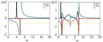
Figure S1: Real and imaginary part of bare susceptibility $\chi^{0}_{\pm}$ as well as the RPA spectra from Eq. (S11) at the momentum $\Gamma$ (a) and $(\pi,\pi/2)$ (b). The data corresponds to $U=2,B=4$ QMC parameter.

At last, we can put it into the RPA formula Eq. (3) in the main text, perform analytical continuation $i\omega_{n}\rightarrow\omega+i\eta^{+}$ and eventually obtain the RPA dynamical spin susceptibility $\chi_{\pm}(\mathbf{q},\omega)$. The spin spectra $S_{\pm}(\mathbf{q},\omega)$ that can be directly compared with QMC+SAC results is

$$S_{\pm}(\mathbf{q},\omega)=\frac{-\text{Im}\chi^{0}_{\pm}(\mathbf{q},\omega)}{[1+U_{\text{eff}}\text{Re}\chi^{0}_{\pm}(\mathbf{q},\omega)]^{2}+[U_{\text{eff}}\text{Im}\chi^{0}_{\pm}(\mathbf{q},\omega)]^{2}}.$$ (S11)

by expanding $\chi_{\pm}$ as a function of $\chi^{0}_{\pm}$.

The origin of the collective Larmor-Silin mode can be elucided from Eq. (S11). To have a pole in the denominator, it requires the bare susceptibility to satisfy $\text{Im}\chi^{0}_{\pm}(\mathbf{q},\omega)\rightarrow 0$ and $\text{Re}\chi^{0}_{\pm}(\mathbf{q},\omega)=\frac{-1}{U_{\text{eff}}}$ simultaneously. It is thus intuitive to find them near the boundary of spectra from bare susceptibility $\chi^{0}_{\pm}$. In Fig. S1, we make the plot of susceptibility at momentum $\Gamma$ and $(\pi,\pi/2)$ as an example. The blue line is the real part of $\chi^{0}_{\pm}$, while the red one is the imaginary part. The black line is the RPA spectra obtained from Eq. (S11). The thin yellow line marks the position of $-1/U_{\text{eff}}$ with $U_{\text{eff}}=1.67$. At the lower boundary of the bare spectra ($-\chi^{0}_{\pm}$), the $-1/U_{\text{eff}}$ thin line crosses the real part of bare susceptibility, giving RPA spectra (the black line) a sharp peak, this is the collective Larmor-Silin mode at this momentum.

Note that the real part of bare susceptibility is not divergent at the boundary of bare spectra, it is intuitive to infer that the condition $\text{Re}\chi^{0}_{\pm}(\mathbf{q},\omega)=\frac{-1}{U_{\text{eff}}}$ could not be satisfied for small enough interaction strength. Therefore, the collective mode might not emerge as soon as we turn on interaction in the model. One will clearly observe the collective mode when sufficient interaction and the polarization of the Dirac dispersions, as shown in the Fig. 3 of the main text. On the other hand, the interaction also shall not be too large, as in that case there would be an interaction driven quantum phase transition into long-ranged ordered state that spontaneously breaks spin $U(1)$ symmetry, and the transverse dynamic susceptibility will give rise to the gapless Goldstone mode at the ordered wave vector ($M(\pi,\pi)$ point in our case).

II Finite-temperature DQMC method and Simulation details

In this work, we use the finite-temperature determinant quantum Monte Carlo (DQMC) method equipped inverse temperature $\beta=L$ to investigate the ground state properties of a $\pi$-flux Hubbard model with on-site interaction and with external magnetic field. In DQMC, we could represent the Hamiltonian – Eq.(1) in main text – as $H=H_{T}+H_{U}$ with noninteracting part $H_{T}=H_{0}+H_{B}$ and interacting part $H_{U}$. The partition function is given as

$$Z=\operatorname{Tr}\left[e^{-\beta H}\right].$$ (S12)

Since $H$ consists of the non-interacting and interacting parts, $H_{T}$ and $H_{U}$, respectively, that are not commute, we should perform Trotter decomposition to discretize inverse temperature $\beta$ into $L_{\tau}$ imaginary time slices ($\beta=L_{\tau}\Delta\tau$), then we have

$$Z=\operatorname{Tr}\left[\left(e^{-\Delta_{\tau}H_{U}}e^{-\Delta_{\tau}H_{0}}\right)^{L_{\tau}}\right]+\mathcal{O}\left(\Delta_{\tau}^{2}\right),$$ (S13)

where the non-interacting and interacting parts of the Hamiltonian are separated. The Trotter decomposition will give rise to a small systematic error $\mathcal{O}(\Delta\tau^{2})$, we need to set $\Delta\tau$ as a small number to get accurate results.

$H_{U}$ contains the quartic fermionic operator that can not be measured directly in DQMC, to deal with that, one need to employ a SU(2) symmetric Hubbard-Stratonovich (HS) decomposition, and the auxiliary fields will couple to the charge density. In our pare, the HS decomposition is

$$e^{-\Delta\tau U(n_{i,\uparrow}+n_{i,\downarrow}-1)^{2}}=\frac{1}{4}\sum_{\{s\}}\gamma(s_{i})e^{\alpha\eta(s_{i})\left(n_{i,\uparrow}+n_{i,\downarrow}-1\right)}+\mathcal{O}\left(\Delta_{\tau}^{4}\right),$$ (S14)

with $\alpha=\sqrt{-\Delta\tau U}$, $\gamma(\pm 1)=1+\sqrt{6}/3$, $\gamma(\pm 2)=1-\sqrt{6}/3$, $\eta(\pm 1)=\pm\sqrt{2(3-\sqrt{6})}$, $\eta(\pm 2)=\pm\sqrt{2(3+\sqrt{6})}$.

Now, the interacting part is transformed into quadratic term but coupled with an auxiliary field. Following simulations are based on the single-particle basis $\bm{c}=\{c_{1},c_{2}\cdots c_{N}\}$, so we can use the matrix notation $K$ and $V$ to represent $H_{T}$ and $H_{U}$ operators. We define the imaginary time propagators

$$U_{s}\left(\tau_{2},\tau_{1}\right)=\prod_{m=m_{1}+1}^{m_{2}}e^{\bm{c}^{\dagger}V\left(s_{m\Delta\tau}\right)\bm{c}}e^{-\Delta_{\tau}\bm{c}^{\dagger}K\bm{c}},$$ (S15)

$$B_{s}\left(\tau_{2},\tau_{1}\right)=\prod_{m=m_{1}+1}^{m_{2}}e^{V\left(s_{m\Delta\tau}\right)}e^{-\Delta_{\tau}K},$$

where $m_{1}\Delta\tau=\tau_{1}$ and $m_{2}\Delta\tau=\tau_{2}$. Then partition function $Z$ can be rewritten as

$$Z=\sum_{\{s_{\tau}\}}\operatorname{Tr}\left[U_{s}(\beta,0)\right]\prod_{m=1}^{M}\gamma(s_{m\Delta\tau})e^{-2\alpha\eta(s_{m\Delta\tau})}=\sum_{\{s_{\tau}\}}\operatorname{det}\left[1+B_{s}(\beta,0)\right]\prod_{m=1}^{M}\gamma(s_{m\Delta\tau})e^{-2\alpha\eta(s_{m\Delta\tau})}.$$ (S16)

Physical observables are measured according to

$$\langle O\rangle=\frac{\operatorname{Tr}\left[\mathrm{e}^{-\beta H}O\right]}{\operatorname{Tr}\left[\mathrm{e}^{-\beta H}\right]}.$$ (S17)

The equal-time single-particle Green function $G_{i,j}(\tau,\tau)$ is given by

$$\left\langle c_{i,\tau}c_{j,\tau}^{\dagger}\right\rangle=\left(1+B_{s}(\tau,0)B_{s}(\beta,\tau)\right)_{i,j}^{-1}.$$ (S18)

and the dynamical single-particle Green function $G_{i,j}(\tau_{1},\tau_{2})$ is given by

$$\left\langle c_{i,\tau_{1}}c_{j,\tau_{2}}^{\dagger}\right\rangle=-\left[\left(\mathbf{1}-\mathbf{G}\left(\tau_{1},\tau_{1}\right)\right)B_{s}^{-1}\left(\tau_{2},\tau_{1}\right)\right]_{i,j}.\qquad\left(\tau_{1}<\tau_{2}\right)$$ (S19)

Other physical observables can be calculated from single-particle Green function through Wick’s theorem. More technical details of the finite-temperature QMC algorithms can be found in the Refs. [80, 73]. In practice, we set inverse temperature $\beta t=16$ for $L=16$ lattice and discrete time slice $\Delta\tau=0.1$.

In order to obtain the transverse spin spectra, we firstly measure dynamical transverse spin correlation function $S_{\pm}(\mathbf{q},\tau)$ Eq. (4) in the main text and then make use of SAC to get real frequency information $S_{\pm}(\mathbf{q},\omega)$. They are related by

$$S_{\pm}(\mathbf{q},\tau)=\int^{\infty}_{0}\mathrm{d}\omega\,K(\tau,\omega)S_{\pm}(\mathbf{q},\omega)$$ (S20)

where $K(\tau,\omega)$ is the kernel. For boson, the kernel $K(\tau,\omega)$ in Eq. (S20) is $\frac{\exp\left(-\tau\omega\right)+\exp\left[-\left(\beta-\tau\right)\omega\right]}{1+\exp\left(-\beta\omega\right)}$ [77]. To get $S_{\pm}(\mathbf{q},\omega)$ which is in the integrand, SAC technique will be applied.

Let’s delve into the intricacies of SAC [76, 78, 77, 81, 82, 83, 1] . The concept involves presenting a highly versatile variational ansatz for the spectrum $S_{\pm}(\mathbf{q},\omega)$ and deriving the associated Green’s function $S_{\pm}(\mathbf{q},\tau)$ in accordance with Eq. (S20). Subsequently, we assess the agreement between the derived Green’s function and the one obtained through QMC, quantified by the parameter $X^{2}(\mathbf{q})$. The definition of $X^{2}(\mathbf{q})$ is then elucidated.

$$X^{2}(\mathbf{q})=\sum_{ij}\left(\bar{S}_{\pm}(\mathbf{q},\tau_{i})-\int^{\infty}_{0}\mathrm{d}\omega\,K(\tau_{i},\omega)S_{\pm}(\mathbf{q},\omega)\right)\left(C^{-1}\right)_{ij}\left(\bar{S}_{\pm}(\mathbf{q},\tau_{j})-\int^{\infty}_{0}\mathrm{d}\omega\,K(\tau_{j},\omega)S_{\pm}(\mathbf{q},\omega)\right)$$ (S21)

where

$$C_{ij}=\frac{1}{N_{b}\left(N_{b}-1\right)}\sum_{b=1}^{N_{b}}\left(S^{b}_{\pm}(\mathbf{q},\tau_{i})-\bar{S}_{\pm}(\mathbf{q},\tau_{i})\right)\left(S^{b}_{\pm}(\mathbf{q},\tau_{j})-\bar{S}_{\pm}(\mathbf{q},\tau_{j})\right)$$ (S22)

and $\bar{S}_{\pm}(\mathbf{q},\tau_{j})$ is the Monte Calro average of Green’s functions of $N_{b}$ bins. $S^{b}_{\pm}(\mathbf{q},\tau_{i})$ is the Monte Carlo measurement of bin b.

Subsequently, we employ Monte Carlo sampling [77, 81] once again to refine the optimization of the spectral function. We assume a specific form for the spectral function: $S_{\pm}(\mathbf{q},\omega)=\sum_{i=1}^{N_{\omega}}A_{i}\delta\left(\omega-\omega_{i}\right)$ where the weight of the Monte Carlo configuration is given by $W\sim\exp\left(-\frac{X^{2}}{2\,\Theta_{T}}\right)$. Here, $\Theta_{T}$ serves as an analogue to temperature. Finally, we calculate the average $\langle X^{2}\rangle$ at different $\Theta_{T}$ through the annealing process. Upon its completion, we can select the converged $\Theta_{T}$ to fulfill the condition:

$$\langle X^{2}\rangle=X_{\min}^{2}+a\sqrt{X_{\min}^{2}}.$$ (S23)

Usually we set $a=2$, and the ensemble average of the spectra at such optimized $\Theta$ is the final one to present in the main text.

References

- Shao et al. [2017] H. Shao, Y. Q. Qin, S. Capponi, S. Chesi, Z. Y. Meng, and A. W. Sandvik, Phys. Rev. X 7, 041072 (2017).
- Rønnow et al. [2001] H. M. Rønnow, D. F. McMorrow, R. Coldea, A. Harrison, I. D. Youngson, T. G. Perring, G. Aeppli, O. Syljuåsen, K. Lefmann, and C. Rischel, Phys. Rev. Lett. 87, 037202 (2001).
- Plihal et al. [1999] M. Plihal, D. L. Mills, and J. Kirschner, Phys. Rev. Lett. 82, 2579 (1999).
- Vollmer et al. [2003] R. Vollmer, M. Etzkorn, P. S. A. Kumar, H. Ibach, and J. Kirschner, Phys. Rev. Lett. 91, 147201 (2003).
- Prabhakar and Stancil [2009] A. Prabhakar and D. D. Stancil, Spin waves: Theory and applications, Vol. 5 (Springer, 2009).
- Feynman [1957] R. P. Feynman, Rev. Mod. Phys. 29, 205 (1957).
- Li et al. [2020] H. Li, Y. D. Liao, B.-B. Chen, X.-T. Zeng, X.-L. Sheng, Y. Qi, Z. Y. Meng, and W. Li, Nature Communications 11, 1111 (2020).
- Landau [2018] L. Landau, in An Introduction to the Theory of Superfluidity (CRC Press, 2018) pp. 185–204.
- Bisset and Blakie [2013] R. N. Bisset and P. B. Blakie, Phys. Rev. Lett. 110, 265302 (2013).
- Blakie et al. [2012] P. B. Blakie, D. Baillie, and R. N. Bisset, Phys. Rev. A 86, 021604 (2012).
- Rybalko et al. [2010] A. Rybalko, S. Rubets, E. Rudavskii, V. Tikhiy, Y. Poluectov, R. Golovashchenko, V. Derkach, S. Tarapov, and O. Usatenko, Journal of Low Temperature Physics 158, 244 (2010).
- Girvin et al. [1986] S. M. Girvin, A. H. MacDonald, and P. M. Platzman, Phys. Rev. B 33, 2481 (1986).
- Lin et al. [2022] X. Lin, B.-B. Chen, W. Li, Z. Y. Meng, and T. Shi, Phys. Rev. Lett. 128, 157201 (2022).
- Pan et al. [2023] G. Pan, X. Zhang, H. Lu, H. Li, B.-B. Chen, K. Sun, and Z. Y. Meng, Phys. Rev. Lett. 130, 016401 (2023).
- Lu et al. [2023a] H. Lu, B.-B. Chen, H.-Q. Wu, K. Sun, and Z. Y. Meng, arXiv e-prints , arXiv:2311.15246 (2023a), arXiv:2311.15246 [cond-mat.str-el] .
- Lu et al. [2023b] H. Lu, H.-Q. Wu, B.-B. Chen, K. Sun, and Z. Y. Meng, arXiv e-prints , arXiv:2401.00363 (2023b), arXiv:2401.00363 [cond-mat.str-el] .
- Nguyen et al. [2022] D. X. Nguyen, F. D. M. Haldane, E. H. Rezayi, D. T. Son, and K. Yang, Phys. Rev. Lett. 128, 246402 (2022).
- Kumar and Haldane [2022] P. Kumar and F. D. M. Haldane, Phys. Rev. B 106, 075116 (2022).
- Balents [2010] L. Balents, Nature 464, 199 (2010).
- Savary and Balents [2017] L. Savary and L. Balents, Phys. Rev. Lett. 118, 087203 (2017).
- Zhou et al. [2017] Y. Zhou, K. Kanoda, and T.-K. Ng, Rev. Mod. Phys. 89, 025003 (2017).
- Kivelson et al. [1987] S. A. Kivelson, D. S. Rokhsar, and J. P. Sethna, Phys. Rev. B 35, 8865 (1987).
- Wen [1991] X. G. Wen, Phys. Rev. B 44, 2664 (1991).
- Wen [2017] X.-G. Wen, Rev. Mod. Phys. 89, 041004 (2017).
- Sun et al. [2018] G.-Y. Sun, Y.-C. Wang, C. Fang, Y. Qi, M. Cheng, and Z. Y. Meng, Phys. Rev. Lett. 121, 077201 (2018).
- Wang et al. [2021a] Y.-C. Wang, M. Cheng, W. Witczak-Krempa, and Z. Y. Meng, Nature Communications 12, 5347 (2021a).
- Xu et al. [2019a] X. Y. Xu, Y. Qi, L. Zhang, F. F. Assaad, C. Xu, and Z. Y. Meng, Phys. Rev. X 9, 021022 (2019a).
- Wang et al. [2019] W. Wang, D.-C. Lu, X. Y. Xu, Y.-Z. You, and Z. Y. Meng, Phys. Rev. B 100, 085123 (2019).
- Huang et al. [2018] C.-J. Huang, Y. Deng, Y. Wan, and Z. Y. Meng, Phys. Rev. Lett. 120, 167202 (2018).
- Wang et al. [2021b] Y.-C. Wang, Z. Yan, C. Wang, Y. Qi, and Z. Y. Meng, Phys. Rev. B 103, 014408 (2021b).
- Geim and Novoselov [2007] A. K. Geim and K. S. Novoselov, Nat. Mater. 6, 183 (2007).
- Hasan and Kane [2010] M. Z. Hasan and C. L. Kane, Rev. Mod. Phys. 82, 3045 (2010).
- Vafek and Vishwanath [2014] O. Vafek and A. Vishwanath, Annu. Rev. Condens. Matter Phys. 5, 83 (2014).
- Mak and Shan [2022] K. F. Mak and J. Shan, Nature Nanotechnology 17, 686 (2022).
- Han et al. [2012] T.-H. Han, J. S. Helton, S. Chu, D. G. Nocera, J. A. Rodriguez-Rivera, C. Broholm, and Y. S. Lee, Nature 492, 406 (2012).
- Wei et al. [2017] Y. Wei, Z. Feng, W. Lohstroh, D. H. Yu, D. Le, C. dela Cruz, W. Yi, Z. F. Ding, J. Zhang, C. Tan, L. Shu, Y.-C. Wang, H.-Q. Wu, J. Luo, J.-W. Mei, F. Yang, X.-L. Sheng, W. Li, Y. Qi, Z. Y. Meng, Y. Shi, and S. Li, arXiv e-prints , arXiv:1710.02991 (2017), arXiv:1710.02991 [cond-mat.str-el] .
- Zeng et al. [2022] Z. Zeng, X. Ma, S. Wu, H.-F. Li, Z. Tao, X. Lu, X.-h. Chen, J.-X. Mi, S.-J. Song, G.-H. Cao, G. Che, K. Li, G. Li, H. Luo, Z. Y. Meng, and S. Li, Phys. Rev. B 105, L121109 (2022).
- Zeng et al. [2023] Z. Zeng, C. Zhou, H. Zhou, L. Han, R. Chi, K. Li, M. Kofu, K. Nakajima, Y. Wei, W. Zhang, D. G. Mazzone, Z. Y. Meng, and S. Li, arXiv e-prints , arXiv:2310.11646 (2023), arXiv:2310.11646 [cond-mat.str-el] .
- Zheng et al. [2023] G. Zheng, Y. Zhu, K.-W. Chen, B. Kang, D. Zhang, K. Jenkins, A. Chan, Z. Zeng, A. Xu, O. A. Valenzuela, J. Blawat, J. Singleton, P. A. Lee, S. Li, and L. Li, arXiv e-prints , arXiv:2310.07989 (2023), arXiv:2310.07989 [cond-mat.str-el] .
- Georgopoulou et al. [2023] M. Georgopoulou, B. Fåk, D. Boldrin, J. R. Stewart, C. Ritter, E. Suard, J. Ollivier, and A. S. Wills, Phys. Rev. B 107, 024416 (2023).
- Liu et al. [2022] J. Liu, L. Yuan, X. Li, B. Li, K. Zhao, H. Liao, and Y. Li, Phys. Rev. B 105, 024418 (2022).
- Arikawa et al. [2006] M. Arikawa, M. Karbach, G. Müller, and K. Wiele, Journal of Physics A: Mathematical and General 39, 10623 (2006).
- Ran et al. [2009] Y. Ran, W.-H. Ko, P. A. Lee, and X.-G. Wen, Phys. Rev. Lett. 102, 047205 (2009).
- Shen et al. [2016] Y. Shen, Y.-D. Li, H. Wo, Y. Li, S. Shen, B. Pan, Q. Wang, H. C. Walker, P. Steffens, M. Boehm, Y. Hao, D. L. Quintero-Castro, L. W. Harriger, M. D. Frontzek, L. Hao, S. Meng, Q. Zhang, G. Chen, and J. Zhao, Nature 540, 559 (2016).
- Kim et al. [1997] D. H. Kim, P. A. Lee, and X.-G. Wen, Phys. Rev. Lett. 79, 2109 (1997).
- Ran et al. [2007] Y. Ran, M. Hermele, P. A. Lee, and X.-G. Wen, Phys. Rev. Lett. 98, 117205 (2007).
- Yan et al. [2021] Z. Yan, Y.-C. Wang, N. Ma, Y. Qi, and Z. Y. Meng, npj Quantum Materials 6, 39 (2021).
- Ma et al. [2018a] N. Ma, G.-Y. Sun, Y.-Z. You, C. Xu, A. Vishwanath, A. W. Sandvik, and Z. Y. Meng, Phys. Rev. B 98, 174421 (2018a).
- Ma et al. [2018b] Z. Ma, J. Wang, Z.-Y. Dong, J. Zhang, S. Li, S.-H. Zheng, Y. Yu, W. Wang, L. Che, K. Ran, S. Bao, Z. Cai, P. Čermák, A. Schneidewind, S. Yano, J. S. Gardner, X. Lu, S.-L. Yu, J.-M. Liu, S. Li, J.-X. Li, and J. Wen, Phys. Rev. Lett. 120, 087201 (2018b).
- Zhu et al. [2018] Z. Zhu, P. A. Maksimov, S. R. White, and A. L. Chernyshev, Phys. Rev. Lett. 120, 207203 (2018).
- Keselman et al. [2020] A. Keselman, L. Balents, and O. A. Starykh, Phys. Rev. Lett. 125, 187201 (2020).
- Balents and Starykh [2020] L. Balents and O. A. Starykh, Phys. Rev. B 101, 020401 (2020).
- Agarwal et al. [2023] M. Agarwal, O. A. Starykh, D. A. Pesin, and E. G. Mishchenko, arXiv e-prints , arXiv:2312.16782 (2023), arXiv:2312.16782 [cond-mat.mes-hall] .
- Silin [1958] V. P. Silin, JETP 6, 945 (1958).
- Silin [1959] V. P. Silin, JETP 8, 870 (1959).
- Platzman and Wolff [1967] P. M. Platzman and P. A. Wolff, Phys. Rev. Lett. 18, 280 (1967).
- Leggett [1970] A. J. Leggett, Journal of Physics C: Solid State Physics 3, 448 (1970).
- van Loon and Strand [2023] E. G. C. P. van Loon and H. U. R. Strand, Communications Physics 6, 289 (2023).
- Schultz and Dunifer [1967] S. Schultz and G. Dunifer, Phys. Rev. Lett. 18, 283 (1967).
- Bercx et al. [2009] M. Bercx, T. C. Lang, and F. F. Assaad, Phys. Rev. B 80, 045412 (2009).
- Otsuka and Hatsugai [2002] Y. Otsuka and Y. Hatsugai, Phys. Rev. B 65, 073101 (2002).
- Chang and Scalettar [2012] C.-C. Chang and R. T. Scalettar, Phys. Rev. Lett. 109, 026404 (2012).
- Parisen Toldin et al. [2015] F. Parisen Toldin, M. Hohenadler, F. F. Assaad, and I. F. Herbut, Phys. Rev. B 91, 165108 (2015).
- Otsuka et al. [2016] Y. Otsuka, S. Yunoki, and S. Sorella, Phys. Rev. X 6, 011029 (2016).
- Ouyang and Xu [2021] Y. Ouyang and X. Y. Xu, Phys. Rev. B 104, L241104 (2021).
- Da Liao et al. [2022a] Y. Da Liao, X. Y. Xu, Z. Y. Meng, and Y. Qi, Phys. Rev. B 106, 075111 (2022a).
- Da Liao et al. [2022b] Y. Da Liao, X. Y. Xu, Z. Y. Meng, and Y. Qi, Phys. Rev. B 106, 115149 (2022b).
- Da Liao et al. [2022c] Y. Da Liao, X. Y. Xu, Z. Y. Meng, and Y. Qi, Phys. Rev. B 106, 155159 (2022c).
- Wen [2007] X. G. Wen, Quantum Field Theory of Many-body Systems : From the Origin of Sound to an Origin of Light and Electrons (Oxford University Press, Oxford, 2007).
- [70] In Sec. I of Supplemental Material, we discuss the details of RPA calculation. Sec. II is devoted to details of DQMC algorithm and HS decomposition.
- Aronov [1977] A. Aronov, Zh. Eksp. Teor. Fiz 73, 577 (1977).
- Blankenbecler et al. [1981] R. Blankenbecler, D. J. Scalapino, and R. L. Sugar, Phys. Rev. D 24, 2278 (1981).
- Xu et al. [2019b] X. Y. Xu, Z. H. Liu, G. Pan, Y. Qi, K. Sun, and Z. Y. Meng, Journal of Physics: Condensed Matter 31, 463001 (2019b).
- Wu and Zhang [2005] C. Wu and S.-C. Zhang, Physical Review B 71, 155115 (2005).
- Pan and Meng [2024] G. Pan and Z. Y. Meng, in Encyclopedia of Condensed Matter Physics (Second Edition), edited by T. Chakraborty (Academic Press, Oxford, 2024) second edition ed., pp. 879–893.
- Sandvik [1998] A. W. Sandvik, Phys. Rev. B 57, 10287 (1998).
- Sandvik [2016] A. W. Sandvik, Phys. Rev. E 94, 063308 (2016).
- Beach [2004] K. Beach, arXiv preprint cond-mat/0403055 (2004).
- Oshikawa and Affleck [2002] M. Oshikawa and I. Affleck, Phys. Rev. B 65, 134410 (2002).
- Assaad and Evertz [2008] F. Assaad and H. Evertz, in Computational Many-Particle Physics, Vol. 739, edited by H. Fehske, R. Schneider, and A. Weiße (Springer Berlin Heidelberg, Berlin, Heidelberg, 2008) pp. 277–356.
- Syljuåsen [2008] O. F. Syljuåsen, Phys. Rev. B 78, 174429 (2008).
- Sandvik [2019] A. W. Sandvik, arXiv preprint arXiv:1909.10591 (2019).
- Shao and Sandvik [2023] H. Shao and A. W. Sandvik, Physics Reports 1003, 1 (2023).