Near-field radiative heat transfer between shifted graphene gratings

Abstract

We examine the near-field radiative heat transfer between finite-thickness planar fused silica slabs covered with graphene gratings, through the utilization of the exact Fourier modal method augmented with local basis functions (FMM-LBF), with focus on the lateral shift effect. To do so, we propose and validate a minor modification of the FMM-LBF theory to account for the lateral shift. This approach goes far beyond the effective medium approximation because this latter cannot account for the lateral shift. We show that the heat flux can exhibit significant oscillations with the lateral shift and, at short separation, it can experience up to a 60%-70% reduction compared to the aligned case. Such a lateral shift effect is found to be sensitive to the geometric factor $d/D$ (separation distance to grating period ratio). When $d/D>2$ (realized through large separation or small grating period), the two graphene gratings see each other as an effective whole rather than in detail, and thus the lateral shift effect on heat transfer becomes less important. Therefore, we can clearly distinguish two asymptotic regimes for radiative heat transfer: the LSE (Lateral Shift Effect) regime, where a significant lateral shift effect is observed, and the non-LSE regime, where this effect is negligible. Furthermore, regardless of the lateral shift, the radiative heat flux shows a non-monotonic dependence on the graphene chemical potential. That is, we can get an optimal radiative heat flux (peaking at about 0.3eV chemical potential) by in situ modulating the chemical potential. This work has the potential to unveil new avenues for harnessing the lateral shift effect on radiative heat transfer in graphene-based nanodevices.

I introduction

Recently, there has been a growing interest in near-field radiative heat transfer (NFRHT), motivated by both fundamental explorations and practical applications. When the separation distance is comparable to or smaller than the thermal wavelength $\lambda_{T}=\hbar c/k_{B}T$, the radiative heat flux can exceed the Planckian blackbody limit by several orders of magnitude [1, 2], due to the near-field effects (e.g., photon tunneling) [3, 4, 5, 6]. The NFRHT has been extensively investigated theoretically for many different geometric configurations [7, 8, 9, 10, 11, 12, 13, 14, 15, 16, 17, 18, 19], some of which have been confirmed by pioneering experimental works [20, 21, 22, 23, 24, 25, 26, 27, 28, 29]. Particularly, when grating structures are involved, they can lead to important enhancement of the NFRHT due to the excitation of high-order diffraction channels [30, 31, 32]. Besides, owing to graphene’s special optical properties, planar graphene-sheet involved structures exhibit many novel behaviors in the radiative heat transfer modulation [33, 34, 35, 36, 37, 38, 39, 40, 41, 42]. It is interesting to know whether the combined richness of the grating geometry and the special dielectric features of graphene could lead to some other novel behavior in NFRHT manipulation that cannot be achieved with conventional materials.

Radiative energy transfer between graphene gratings based structures [43, 44, 45] has recently been investigated, where patterning the graphene sheets has been found to open more energy transfer channels. All of these works consider two perfectly aligned and identically patterned graphene structures. The effect of twisted grating has also been investigated [46, 47, 48]. Still, the effect of a lateral shift between the two parallel gratings remains unexplored. Introducing a lateral shift will allow a modulation of the near-field radiative heat transfer keeping constant the separation distance. It is worth stressing that the effective medium theory (EMT), that is often used to study the NFRHT between substrate-supported graphene strips [49], treats the graphene grating as an effective whole and thus cannot account for the lateral shift effect. The study of a shifted configuration needs an exact numerical method to treat the electromagnetic wave scattering by the gratings.

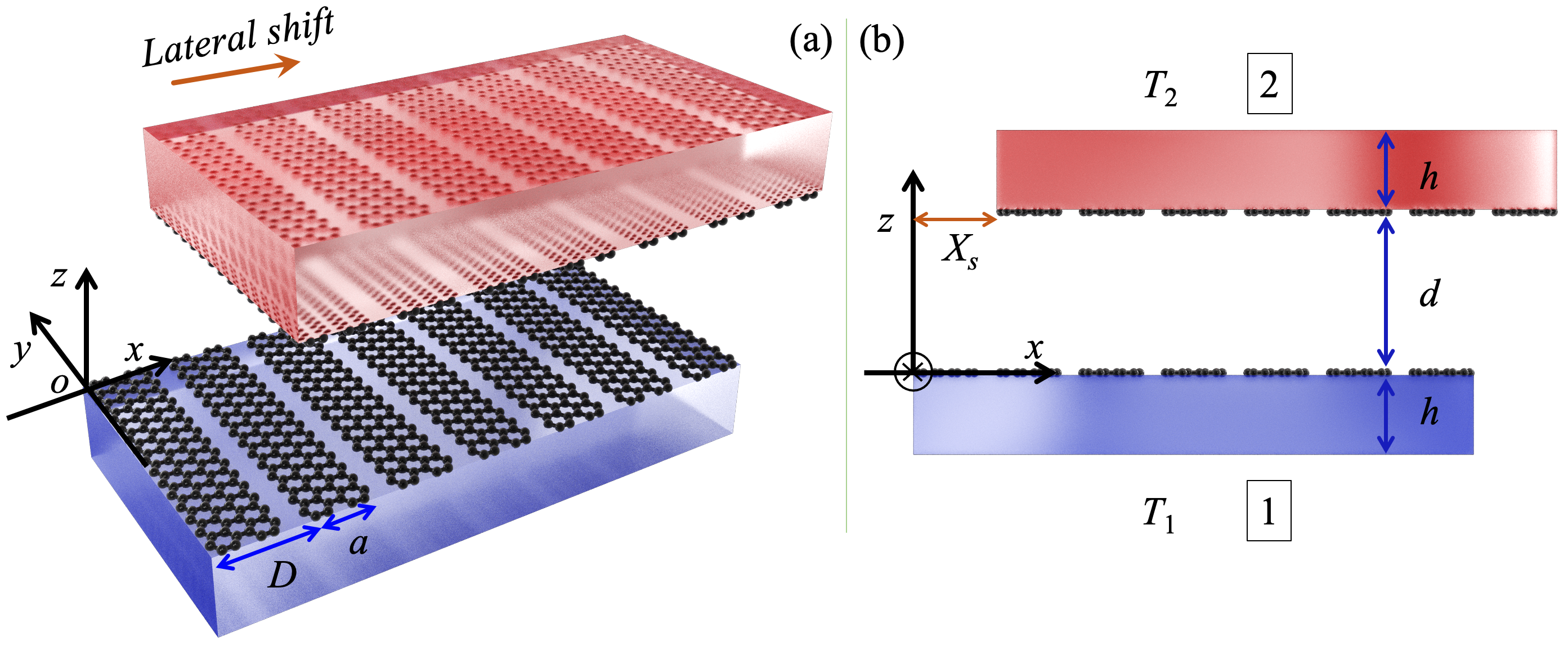
Figure 1: Structure diagram of the supported graphene gratings considering relative lateral shift $X_{s}$: (a) the main view and (b) the side view.

In this work we investigate the effect of a lateral shift on NFRHT. We will consider planar fused silica slabs coated with graphene gratings (see Fig. 1). Concerning the numerical investigations, we will use an exact method: the Fourier modal method equipped with local basis functions (FMM-LBF), which is particularly efficient for one-dimensional strip gratings [50, 51, 52, 53]. In order to take into account this lateral shift, besides the existing method of including the lateral shift by directly applying the reference translation to the scattering operators [54], and we check our results by using a second method to include the lateral shift effect in the scattering operators themselves.

This work is organized as follows: In Sec. II, the physical model of the planar fused silica slabs covered with graphene gratings with a relative lateral shift and the theoretical models of the scattering approach for radiative heat transfer are presented. In Sec. III, the effects of influencing factors (e.g., grating period, chemical potential and filling fraction) on the lateral shift mediated NFRHT are analyzed, and asymptotic regimes of the lateral shift effect are also proposed.

II Theoretical models

The physical system is shown in Fig. 1. We investigate the NFRHT between bodies 1 and 2. The relative lateral displacement between the two graphene strips along the $x$-axis is $X_{s}$. When $X_{s}=0$, the two graphene gratings are perfectly aligned and the near-field radiative heat transfer, in this case, has been recently investigated (please refer to our recent work for more details [45]).
In the following, we will denote by $D$ the graphene grating period, by $a$ the width of one single graphene strip, by $h$ the common thickness of the planar slabs and by $d$ the separation distance between the two gratings. Bodies 1 and 2 are considered at fixed temperatures $T_{1}$ and $T_{2}$, respectively, while the environment is at the same temperature as body 1. The electromagnetic properties of graphene are taken into account through its conductivity $\sigma_{g}$ which depends on the temperature $T$ and on the chemical potential $\mu$. It is the sum of an intraband and an interband contributions $\left(\sigma_{g}=\sigma_{\textnormal{intra}}+\sigma_{\textnormal{inter}}\right)$ given by [37, 55, 56, 57]:

$$\sigma_{\textnormal{intra}}=\frac{i}{\omega+i/\tau}\frac{2e^{2}k_{\rm B}T}{\pi\hbar^{2}}\ln\left[2\cosh\left(\dfrac{\mu}{2k_{\rm B}T}\right)\right],$$ (1)

and

$$\sigma_{\textnormal{inter}}=\frac{e^{2}}{4\hbar}\left[G\left(\frac{\hbar\omega}{2}\right)+i\dfrac{4\hbar\omega}{\pi}\int_{0}^{+\infty}\dfrac{G(\xi)-G\left(\hbar\omega/2\right)}{(\hbar\omega)^{2}-4\xi^{2}}{\rm d}\xi\right],$$ (2)

where $e$ is the electron charge, $\tau$ the relaxation time (we use $\tau=10^{-13}$s) and $G(\xi)=\sinh(\xi/k_{B}T)/[\cosh(\mu/k_{\rm B}T)+\cosh(\xi/k_{\rm B}T)]$.

The net power flux $\varphi$ received by body 1 (energy per unit surface and time) can be defined as [58, 54]

$$\varphi=\sum_{p}\int\frac{{\rm d}^{2}{\rm\textbf{k}}}{(2\pi)^{2}}\int_{0}^{+\infty}(\Theta(\omega,T_{2})-\Theta(\omega,T_{1}))\frac{{\rm d}\omega}{2\pi}<p,{\rm\textbf{k}}|\mathcal{O}|p,{\rm\textbf{k}}>,$$ (3)

where $p$ is the polarization index, $p=$ 1, 2 corresponding to TE (transverse electric) and TM (transverse magnetic) polarization modes respectively, $\Theta(\omega,T)=\hbar\omega/(e^{{\hbar\omega}/{k_{\rm B}T}}-1)$ is the mean energy of the Planck oscillator, $\hbar$ is the reduced Planck constant, $\omega$ is the angular frequency, $k_{\rm B}$ is the Boltzmann constant, ${\rm\textbf{k}}=(k_{x},k_{y})$, $k_{x}$ and $k_{y}$ being the wave vectors in the standard $(x,y,z)$ cartesian coordinates system. The transmission operator $\mathcal{O}$ in the (TE, TM) basis is given by [54]

$$\mathcal{O}=U^{(2,1)}\left[f_{-1}(\mathcal{R}^{(2)-})-\mathcal{T}^{(2)-}\mathcal{P}_{-1}^{({\rm pw})}\mathcal{T}^{(2)-\dagger}\right]U^{(2,1){\dagger}}\left[f_{1}(\mathcal{R}^{(1)+})-\mathcal{T}^{(1)-\dagger}\mathcal{P}_{1}^{({\rm pw})}\mathcal{T}^{(1)-}\right],$$ (4)

where $U^{(2,1)}=\left(1-\mathcal{R}^{(2)-}\mathcal{R}^{(1)+}\right)^{-1}$, $\mathcal{R}^{(1)+}$ and $\mathcal{R}^{(2)-}$ ($\mathcal{T}^{(1)-}$ and $\mathcal{T}^{(2)-}$ ) are the reflection operators (transmission operators) of grating 1 and grating 2 in the (TE, TM) basis, $\dagger$ stands for the conjugation operation and the $\pm$ superscripts in the reflection and transmission coefficients correspond to the propagation direction with respect to the $z$ axis. $\left\langle p,{\textbf{k}}|\mathcal{P}_{\zeta}^{\rm(pw/ew)}|p^{\prime},{\textbf{k}}^{\prime}\right\rangle=k_{z}^{\zeta}\left\langle p,{\textbf{k}}|\mathcal{\prod}^{\rm(pw/ew)}|p^{\prime},{\textbf{k}}^{\prime}\right\rangle$, $k_{z}=\sqrt{k_{0}^{2}-\textbf{k}^{2}}$, $k_{0}=\omega/c$, $\mathcal{\prod}^{\rm(pw)}$ ($\mathcal{\prod}^{\rm(ew)}$) is the projector on the propagative (evanescent) sector, and the auxiliary function $f_{\alpha}(\mathcal{R})$ is given by [58, 54]:

$$f_{\zeta}(\mathcal{R})=\left\{\begin{array}[]{rcl}\mathcal{P}_{-1}^{(\rm pw)}-\mathcal{R}\mathcal{P}_{-1}^{(\rm pw)}\mathcal{R}^{\dagger}+\mathcal{R}\mathcal{P}_{-1}^{(\rm ew)}-\mathcal{P}_{-1}^{(\rm ew)}\mathcal{R}^{\dagger}&&\zeta=-1,\\ \\ \mathcal{P}_{1}^{(\rm pw)}-\mathcal{R}^{\dagger}\mathcal{P}_{1}^{(\rm pw)}\mathcal{R}+\mathcal{R}^{\dagger}\mathcal{P}_{1}^{(\rm ew)}-\mathcal{P}_{1}^{(\rm ew)}\mathcal{R}&&\zeta=1.\end{array}\right.$$ (5)

According to Ref. [31], the periodicity along the $x$ axis makes it natural to replace the mode variable $k_{x}$ with $k_{xn}=k_{x}+n\frac{2\pi}{D}$, and $k_{z}$ becomes $k_{zn}=\sqrt{k_{0}^{2}-k_{xn}^{2}-k_{y}^{2}}$, where $n\in\mathbb{Z}$, $k_{x}$ is in the first Brillouin zone $(-\frac{\pi}{D},\frac{\pi}{D})$, and $k_{y}\in\mathbb{R}$.

The reflection and transmission operators $\mathcal{R}^{(1)+}$, $\mathcal{R}^{(2)-}$, $\mathcal{T}^{(1)-}$ and $\mathcal{T}^{(2)-}$, needed for our calculations, are obtained from the operators $\mathcal{R}$ and $\mathcal{T}$ corresponding to the reference structure shown in Fig. 2 and whose derivation is detailed in the appendix.

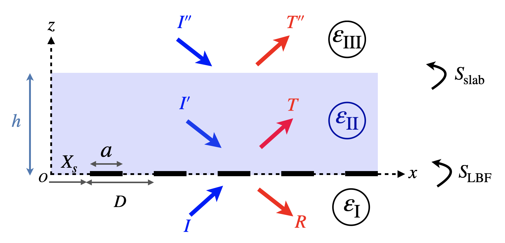
Figure 2: Reference structure used in the computation of the different reflection and transmission operators.

Body 1 has no lateral shift, $i.e.$, $X_{s}=0$. Then $\mathcal{R}^{(1)+}$ and $\mathcal{T}^{(1)-}$ at the interface $z=0$ and with no lateral shift $X_{s}=0$ (see Fig. 1) can be obtained directly from the known $\mathcal{R}^{-}$ and $\mathcal{T}^{+}$ by using the following relations [31, 45]:

$$\begin{split}&\left\langle p,{\textbf{k}},n|\mathcal{R}^{(1)+}(\omega)|p^{\prime},{\textbf{k}}^{\prime},n^{\prime}\right\rangle\\ &=\left\{\begin{array}[]{rcl}\begin{aligned} &\left\langle p,{\textbf{k}},n|\mathcal{R}^{-}(\omega)|p,{\textbf{k}}^{\prime},n^{\prime}\right\rangle&p=p^{\prime}\\ &-\left\langle p,{\textbf{k}},n|\mathcal{R}^{-}(\omega)|p^{\prime},{\textbf{k}}^{\prime},n^{\prime}\right\rangle&p\neq p^{\prime},\end{aligned}\end{array}\right.\end{split}$$ (6)

and

$$\begin{split}&\left\langle p,{\textbf{k}},n|\mathcal{T}^{(1)-}(\omega)|p^{\prime},{\textbf{k}}^{\prime},n^{\prime}\right\rangle\\ &=\left\{\begin{array}[]{rcl}\begin{aligned} &\left\langle p,{\textbf{k}},n|\mathcal{T}^{+}(\omega)|p,{\textbf{k}}^{\prime},n^{\prime}\right\rangle,p=p^{\prime}\\ &-\left\langle p,{\textbf{k}},n|\mathcal{T}^{+}(\omega)|p^{\prime},{\textbf{k}}^{\prime},n^{\prime}\right\rangle,p\neq p^{\prime}.\end{aligned}\end{array}\right.\end{split}$$ (7)

As for body 2, there is, not only, a lateral shift $X_{s}$ but an interface translation to $z=d$ (see Fig. 1). In order to take into account these two kinds of translation and obtain $\mathcal{R}^{(2)-}$ and $\mathcal{T}^{(2)-}$ one can consider two methods. The first one consists in directly applying appropriate translation operators to the scattering operators. This approach has been discussed, in detail, in a previous work [54] from which we take the results giving $\mathcal{R}^{(2)-}$ and $\mathcal{T}^{(2)-}$ in terms of $\mathcal{R}^{-}$ and $\mathcal{T}^{-}$:

$$\left\{\begin{array}[]{rcl}\begin{aligned} &\left\langle p,{\textbf{k}},n|\mathcal{R}^{(2)-}(\omega)|p^{\prime},{\textbf{k}}^{\prime},n^{\prime}\right\rangle\\ &=e^{i\left(k_{xn^{\prime}}^{\prime}-k_{xn}\right)X_{s}}e^{i\left(k_{zn}+k_{zn^{\prime}}^{\prime}\right)d}\left\langle p,{\textbf{k}},n|\mathcal{R}^{-}(\omega)|p^{\prime},{\textbf{k}}^{\prime},n^{\prime}\right\rangle,\\ &\left\langle p,{\textbf{k}},n|\mathcal{T}^{(2)-}(\omega)|p^{\prime},{\textbf{k}}^{\prime},n^{\prime}\right\rangle\\ &=e^{i\left(k_{xn^{\prime}}^{\prime}-k_{xn}\right)X_{s}}e^{i\left(k_{zn}-k_{zn^{\prime}}^{\prime}\right)d}\left\langle p,{\textbf{k}},n|\mathcal{T}^{-}(\omega)|p^{\prime},{\textbf{k}}^{\prime},n^{\prime}\right\rangle.\end{aligned}\end{array}\right.$$ (8)

The second one, consists in incorporating the effect of the lateral shift directly in the computation of the scattering operators $\mathcal{R}^{-}$ and $\mathcal{T}^{-}$ with the FMM-LBF (as given in the appendix), and then applying the translation operator (as previously) only in the $z$ direction.

It is important to stress that these two approaches are completely equivalent. A numerical verification of this is shown in Fig. 3 where we compute the radiative heat flux spectrum for the structure shown in Fig. 1, using the two methods (the different parameters are given in the caption). As can be seen from the figure, there is a very good agreement between the two approaches and a closer look at the data reveals that the results are identical to our working precision. Therefore, either of these methods can be used in the investigations to come.

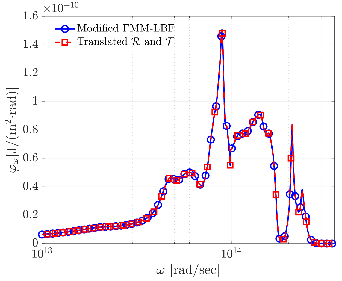
Figure 3: The radiative heat flux spectrum of the configuration shown in Fig. 1 using SiO₂ slabs (whose optical data are taken from Ref.[59]), $\mu=0.3$ eV, a lateral shift $X_{s}=0.5\mu$m and a grating period $D=2\mu$m at separation distance $d=100$ nm, with $T_{1}=290$K and $T_{2}=310$K, obtained by the two different approaches : (1) the modified FMM-LBF and (2) the translated scattering operators

III Results and discussion

In this section, we use the theoretical model outlined above to investigate the NFRHT between the slabs of Fig. 1. Parametric investigations of influencing factors on NFRHT will be performed and a particular interest will be given to the asymptotic regimes for the lateral shift effect. In the following, bodies 1 and 2 are maintained at $T_{1}=290$K and $T_{2}=310$K, respectively. The truncation order $N$, used in the FMM-LBF, is fixed at 30 to ensure convergent results. The substrate thickness $h$ is fixed at 20 nm.

III.1 Parametric investigation of influencing factors on lateral-shift-induced NFRHT: grating period, chemical potential and filling fraction

We consider three different influencing factors that may affect the effect of relative lateral shift between the two gratings on its heat transfer: the grating period $D$, the chemical potential $\mu$ of graphene and the filling fraction $f$. We start the parametric investigation with the grating period $D$. In Fig. 4 (a), we show the dependence of heat flux $\varphi$ on the relative lateral shift $X_{s}$. Three different periods are considered, $D=100$nm, 500nm and 1000nm, respectively. The other parameters are $f=0.5$, $d=100$nm, and $\mu=0.5$eV.

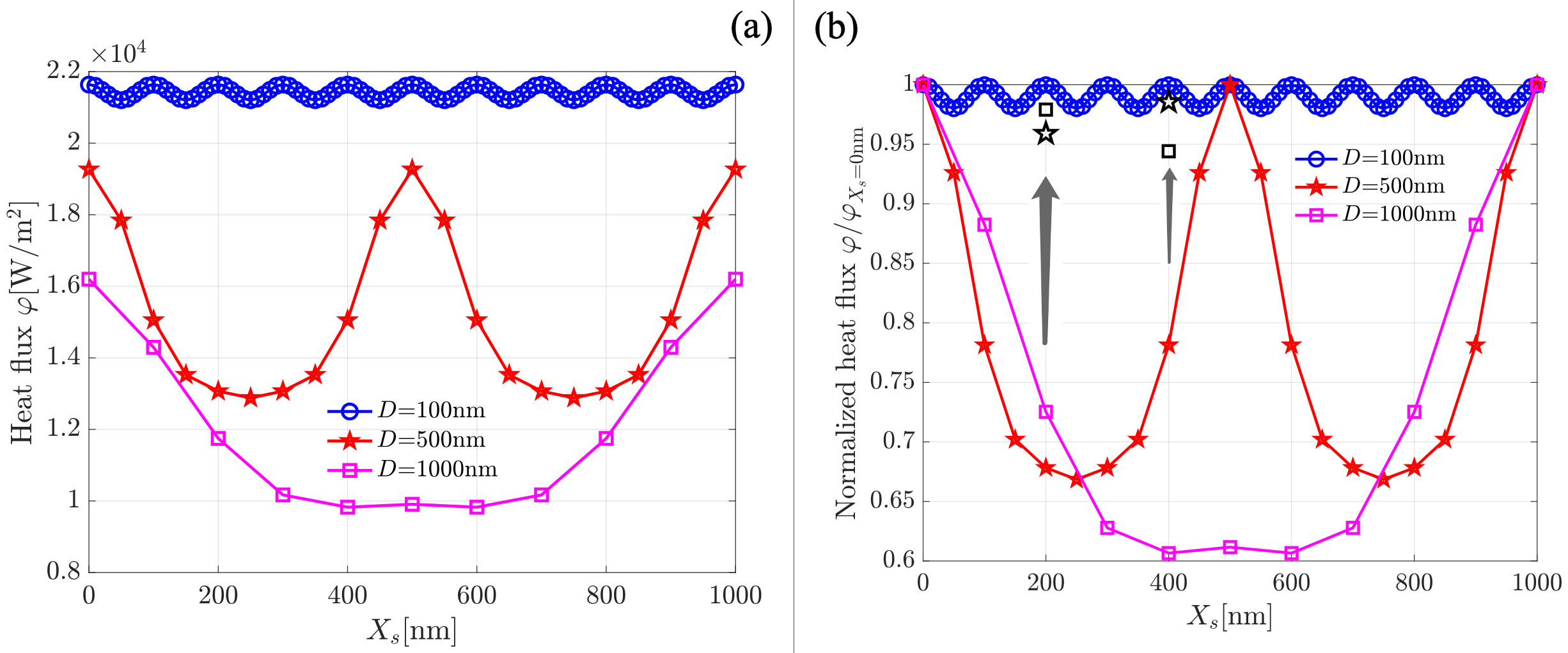
Figure 4: Dependence of heat flux $\varphi$ and normalized heat flux $\varphi/\varphi(X_{s}=0\text{nm})$ on the relative lateral shift $X_{s}$: (a) the absolute heat flux $\varphi$ and (b) ratio of the heat flux $\varphi$ to the heat flux at $X_{s}=0$nm. Three different periods are considered, $D=100$nm, 500nm and 1000nm.

When shifting one of the grating, we can observe a periodic oscillation of the radiative heat flux with the same spatial period as the grating itself. As shown in Fig. 4 (a), for a fixed lateral shift $X_{s}$, the radiative heat flux decreases by about 30% when the period $D$ increases from 100nm to 1000nm. Additionally, the oscillation amplitude of the radiative heat flux induced by the lateral shift increases significantly with increasing period $D$. To show the change of the oscillation amplitude corresponding to different grating periods, we normalize the radiative heat flux $\varphi(X_{s})$ by $\varphi(X_{s}=0\text{nm})$ (i.e. the one without a lateral shift). The result is shown in Fig. 4 (b). Lateral shift affects the heat transfer significantly. For the case where $D=1000$nm, the lateral shift can even result in 40% reduction of the heat flux. While for the case where $D=100$nm, the lateral shift can reduce it by only few percent, which is negligible compared to that for the case of a large spatial period ($D=1000$nm and 500nm). For a fixed separation distance $d$, the scattering details become more important when increasing the grating period $D$ (and thus the ratio $D/d$), causing the nanostructures ”see” each other in more detail. In such a situation, a full and exact theory is needed to account for the complexity of the nanostructures and be able to compare with experiments while the effective medium theory becomes completely invalid.

In our recent paper [53], when discussing the non-additivity of the Casimir force (a kind of geometric effect) between two aligned graphene grating coated finite-size fused silica slabs, (the same configuration as in this work but with no lateral shift), we introduced a dimensionless parameter $d/D$ and proved its relevance to such a kind of geometric effect. The effect of the relative lateral shift on the NFRHT is also geometry related, therefore, we want to know if the dimensionless parameter $d/D$ is still pertinent in this case. The three curves in Fig. 4 (b) correspond to a fixed separation distance $d=100$nm, where the $d/D=1$, 0.2 and 0.1 for the cases $D=100$nm, 500nm and 1000nm, respectively. To verify the relevance of $d/D$ to the lateral shift effect, we performed additional calculations using the couples ($d=500$nm, $D=500$nm) and ($d=1000$nm, $D=1000$nm) to in order to maintain $d/D=1$ as for the case ($d=100$nm, $D=100$nm) already shown. Two lateral shift distances $X_{s}=200$nm and 400nm are considered. The results are added in Fig. 4 (b) and shown as the star and square symbols in black for period $D=500$nm and 1000nm respectively. We see that they both move close to the $d=100$nm and $D=100$nm curve, confirming the relevance of the geometric factor $d/D$ and hence of the geometric nature of the effect.

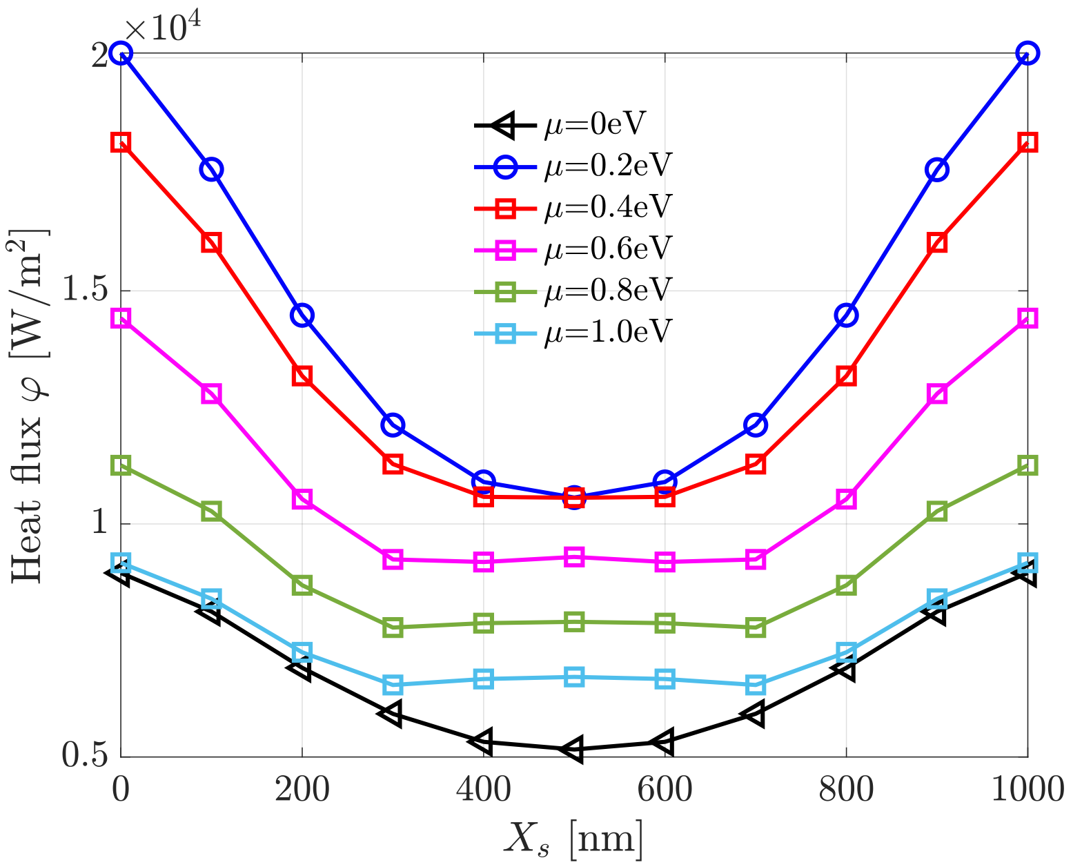
Figure 5: Dependence of radiative heat flux $\varphi$ on the lateral shift $X_{s}$. The chemical potential $\mu=0$eV, 0.2eV, 0.4eV, 0.6eV, 0.8eV and 1.0eV. The period $D=1000$nm, filling fraction $f=0.5$, separation distance $d=100$nm.

We then study the effect of the chemical potential $\mu$ of graphene on the NFRHT. We show the dependence of heat flux $\varphi$ on the relative lateral shift $X_{s}$ in Fig. 5, considering different chemical potential values $\mu=0$eV, 0.2eV, 0.4eV, 0.6eV, 0.8eV and 1.0eV with $D=1000$nm, $f=0.5$ and $d=100$nm. The upper body 2 is laterally shifted in the range of one full grating spatial period. At different Fermi levels, the lateral shift effect on the NFRHT changes slightly. When the chemical potential is not too small ($e.g.,\mu>0.2$eV), when laterally shifting body 2, the radiative heat flux decreases to reach a valley, then keeps constant for a range of lateral shifts (forming a plateau), and finally increases to the same value as that without lateral shift. While for the chemical potential $\mu=0$eV and 0.2eV, radiative heat flux will decrease to reach the valley and then increase directly and go back to that of no lateral shift. Fig. 5 also indirectly shows that the radiative heat flux is not monotonic with the chemical potential (this behavior will be studied in detail in Fig. 6). A natural question is whether we can obtain an optimal radiative heat flux by choosing an appropriate chemical potential $\mu$ for graphene gratings.

To answer the above question, we calculated the dependence of the radiative heat flux $\varphi$ on the chemical potential $\mu$ for different lateral shifts $X_{s}=0$nm, 100nm, 200nm, 300nm, 400nm and 500nm, for $D=1000$nm, $f=0.5$ and $d=100$nm. The results are reported in Fig. 6 where we see that when increasing the chemical potential, the radiative heat flux increases at first to its peak and then decreases gradually for all considered lateral shift $X_{s}$ curves. For the considered separation $d$ and grating period $D$, the radiative heat flux appears to be optimal for $\mu$ at around $0.25$eV.

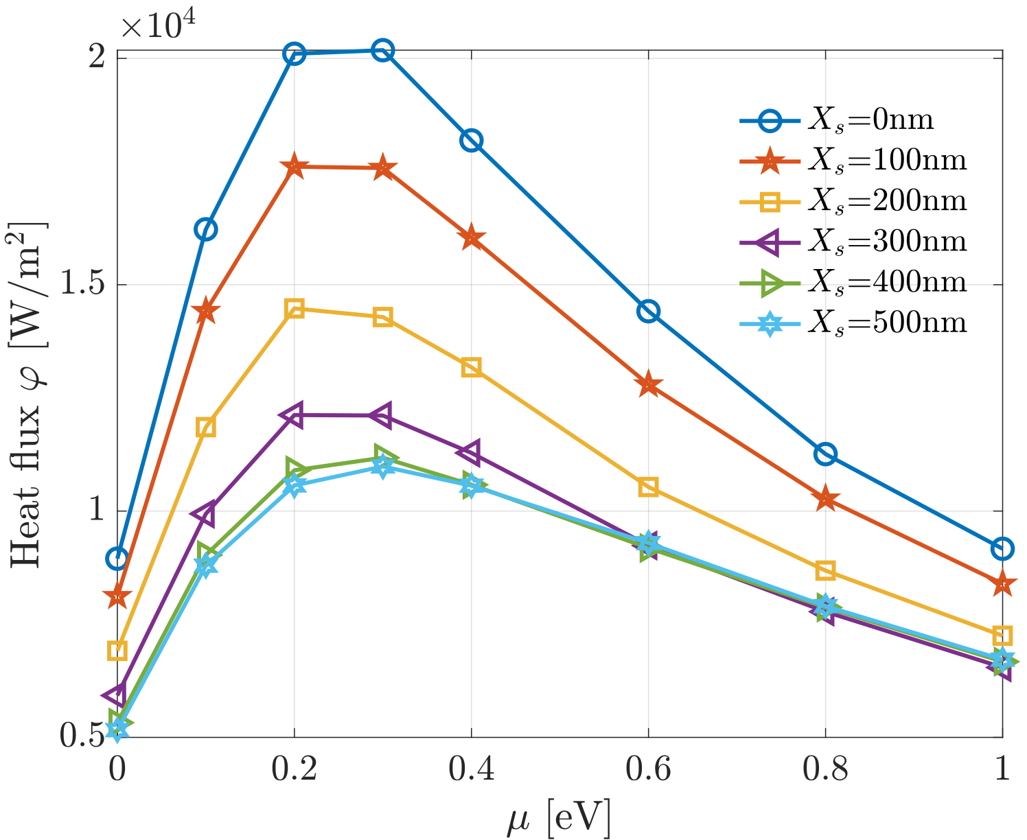
Figure 6: Dependence of radiative heat flux $\varphi$ on the chemical potential $\mu$ of graphene. The lateral shift $X_{s}=0$nm, 100nm, 200nm, 300nm, 400nm and 500nm, period $D=1000$nm, filling fraction $f=0.5$, separation distance $d=100$nm.

Additionally, we study the effect of the filling fraction $f$ on the NFRHT. We show the dependence of heat flux on the filling fraction in Fig. 7 (a) where five different filling fractions are considered, $f$ = 0, 0.2, 0.5, 0.8 and 1.0 with $d=1000$nm and $D=1000$nm. For $f$ = 0 and 1.0, the configurations reduce to the bare/coated slab cases. As expected, the heat flux for these two cases is independent on the lateral shift. At a large separations (e.g., $d=1000$nm), adding a graphene sheet coating on the fused silica substrate (right triangle green line) will significantly enhance the radiative heat flux as compared to the bare fused silica substrate (left triangle black line), which is consistent with the observations in references [45, 33]. At short separations and without considering any lateral shift, as reported in our recent work [45], patterning graphene from a sheet to a grating, can significantly enhance the heat flux. However, at large separations, the patterning method does not always work to enhance heat flux. As shown in Fig. 7 (a), by comparing the curves for $f=0.2$, 0.5 and 0.8 to the curve for $f=1.0$, we can clearly see that, apart from the enhancement seen for $f=0.8$, the patterning method fails to enhance the heat flux. Moreover, when laterally shifting the upper body 2 in the case $f=0.8$, the heat flux will become less than that of the graphene sheet coating case ($f=1.0$) (for $X_{s}\in[200,800]$nm).

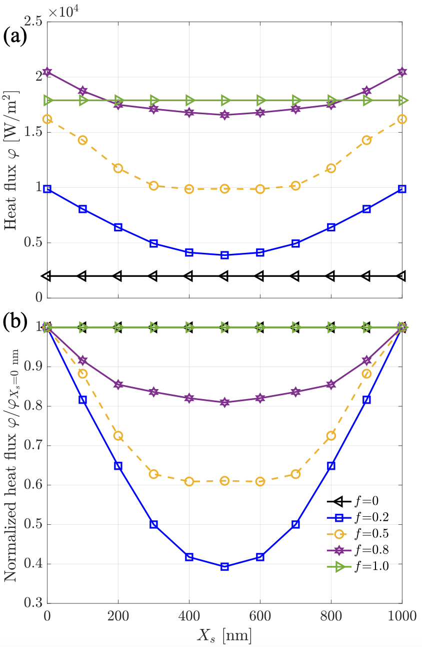
Figure 7: Dependence of heat flux $\varphi$ and normalized heat flux $\varphi/\varphi(X_{s}=0\text{nm})$ on the relative lateral shift $X_{s}$: (a)the absolute heat flux $\varphi$ and (b) ratio of the heat flux $\varphi$ to the heat flux at $X_{s}=0$nm. Five different filling fractions are considered, $f$ = 0, 0.2, 0.5, 0.8 and 1.0, respectively. The separation distance $d=100$nm, grating period $D=1000$nm, chemical potential $\mu=0.5$eV.

in Fig. 7 (b), we show the dependence of the ratio $\varphi(X_{s})/\varphi(X_{s}=0)$ on the filling fraction $f$. As expected, it is constant an equal to 1 for both $f=0$ and 1. For the other filling fractions, this ratio decreases from 1 to a valley value and then increases back to 1. For a lateral shift about 500nm, the heat flux can even experience up to 60% reduction when $f=0.2$. Considering that both the scale of the lateral shift and the geometry, considered here, are realistic and experimentally accessible, the lateral-displacement-sensitive radiative heat transfer might have potential for thermal logic gates applications.

III.2 Asymptotic regimes for the lateral shift effect on NFRHT

In this section, we try to find an asymptotic regime map for the lateral shift effect on NFRHT between substrate-supported graphene gratings to quickly tell the existence of the lateral shift effect or not. Considering that the relevance of the dimensionless geometric factor $d/D$ for the lateral shift effect has been confirmed in Section III.1, we may take advantage of it to propose the asymptotic regime map.

According to the above analysis, for a fixed separation $d$, the lateral shift of the upper body 2 by a half period will have the maximum reduction of heat flux. We also analyzed the effect of the chemical potential $\mu$ and the filling fraction $f$ on the lateral shift effect for the configurations of a fixed separation $d$ and graphene grating period $D$. As shown in Fig. 5, the lateral shift effect on the heat flux is significant no matter how large or small the chemical potential is. However, as shown in Fig. 7, the lateral shift effect on the heat flux is highly sensitive to the filling fraction. That is, as the filling fraction $f$ approaches 0 or 1, the lateral shift effect disappears. Hereinafter, we will use the ratio of heat flux with a half period shift $\varphi(X_{s}=0.5D)$ to that without a shift $\varphi(X_{s}=0)$ to evaluate the lateral shift effect on heat flux.

We will, first, check whether the filling fraction affects the asymptotic regime. The dependence of the ratio $\varphi(X_{s}=0.5D)/\varphi(X_{s}=0)$ on the separation distance $d$ is shown in Fig. 8 where five different filling fractions are considered : $f$ = 0.1, 0.3, 0.5, 0.7 and 0.9. The grating period is $D=100$nm and the chemical potential is $\mu=0.5$eV. We can see a clear dependance of the ratio $\varphi(X_{s}=0.5D)/\varphi(X_{s}=0)$ on $d$ with two distinct regime zones: (i) the first one for $d\leq 200$nm where the ratio varies quickly and (ii) the second one for $d\geq 200$nm where the ratio is almost constant. Moreover, we remark that even for small period configurations (i.e., 100nm), the lateral shift can still have a wide range modulation of the heat flux, with a maximum reduction of 30% (in the first zone).

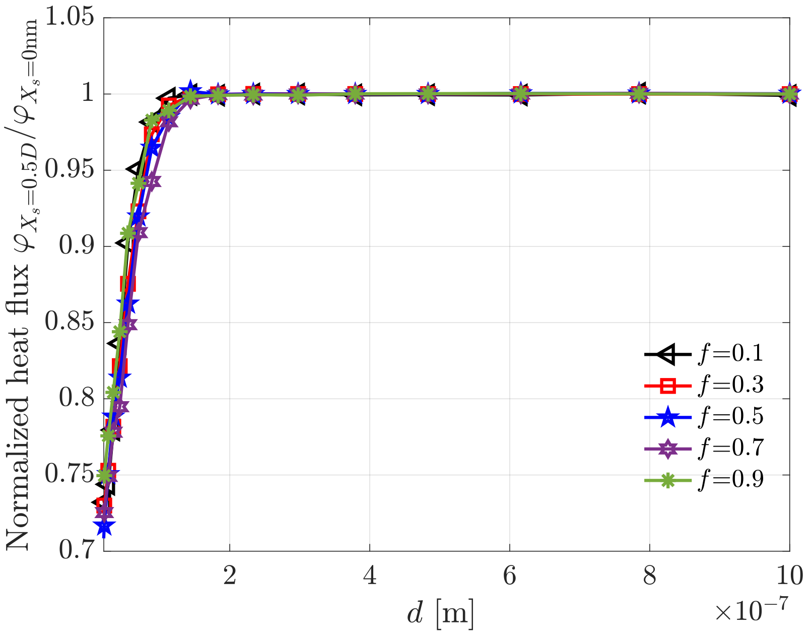
Figure 8: Dependence of normalized heat flux $\varphi_{X_{s}=0.5D}/\varphi_{X_{s}=0\text{nm}}$ on separation distance $d$. Five different filling fractions are considered, $f$ = 0.1, 0.3, 0.5, 0.7 and 0.9, respectively. The grating period $D=100$nm, chemical potential $\mu=0.5$eV.

Beyond the separation point $d=200$nm, the lateral shift effect becomes less important. In addition, such a critical separation point does not change with the filling fraction $f$. To understand why the lateral shift effect on heat transfer changes with the separation $d$, we show the energy transmission coefficient Tr($\mathcal{O}$) in the ($k_{x}/k_{0}$, $k_{y}/k_{0}$) plane at the angular frequency $\omega=5\times 10^{13}$rad/s (where the contribution of graphene to the NFRHT spectrum is important) for a slab coated with a graphene grating in Fig. 9. Tr($\mathcal{O}$) is the sum over the two polarizations of the photon tunneling probabilities, which is usually applied to analyze the mechanisms behind the NFRHT [60, 61, 45]. The transmission coefficient operator $\mathcal{O}$ is defined by Eq. (4). In Fig. 9, four configurations are considered: (a) $d=20$nm and $X_{s}=0$nm, (b) $d=20$nm and $X_{s}=50$nm, (c) $d=200$nm and t $X_{s}=0$nm, and (d) $d=200$nm and $X_{s}=50$nm, together with $D=100$nm, $\mu=0.5$eV and $f$=0.5. The dotted curves represent the dispersion relations obtained from the poles of the reflection coefficient [49, 62].

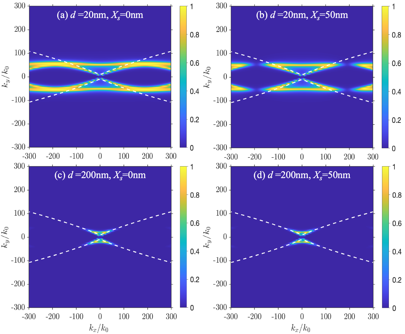
Figure 9: Energy transmission coefficient for a fused silica substrate coated with a graphene grating: (a) separation $d=20$nm and lateral shift $X_{s}=0$nm, (b) separation $d=20$nm and lateral shift $X_{s}=50$nm, (c) separation $d=200$nm and lateral shift $X_{s}=0$nm, and (d) separation $d=200$nm and lateral shift $X_{s}=50$nm. The grating period $D=100$nm, chemical potential $\mu=0.5$eV, filling fraction $f$=0.5.

For the configurations with $d=200$nm, the topology of the accessible modes does not change with the lateral shift, as shown in Fig. 9 (c) and (d). However, for $d=20$nm, the topology of the accessible modes changes slightly, as shown in Fig. 9 (a) and (b). There are more accessible high-$k$ modes for the case with no lateral shift than that for the case with a half-period lateral shift, which accounts for the fact that the radiative heat flux decreases significantly as the upper body 2 moves from the aligned situation to the misaligned one. Whether the lateral shift exists or not, the supported surface plasmon polariton is alway the hyperbolic one. Compared to the transition from circular one to the hyperbolic one by patterning the graphene sheet into a grating, the lateral shift will not induce a critical topology transition, but only slightly affect the accessible range of high-$k$ modes.

Now, we investigate and determine the asymptotic regime map for the lateral shift effect by using the geometric factor $d/D$. For that, we take the typical filling fraction $f=0.5$ and chemical potential $\mu=0.5$eV. In Fig. 10 we show the ratio $\varphi_{X_{s}=0.5D}/\varphi_{X_{s}=0\text{nm}}$ in the ($d,D$) plane where the black dotted lines corresponding to the lines representing the geometric factor $d/D=0.5$, 1.0 and 2.0 are added for reference.

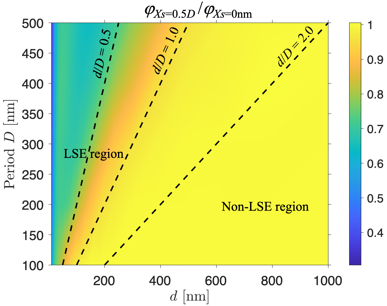
Figure 10: Dependence of the ratio $\varphi_{X_{s}=0.5D}/\varphi_{X_{s}=0\text{nm}}$ on separation distance $d$ and grating period $D$. The filling fraction $f$ = 0.5, chemical potential $\mu=0.5$eV. The dotted lines (geometric factor $d/D=0.5$, 1.0 and 2.0, respectively) are added for reference.

For a given grating period $D$, as the separation $d$ becomes large enough, the ratio $\varphi_{X_{s}=0.5D}/\varphi_{X_{s}=0\text{nm}}$ approaches 1 and the scattering details of the graphene grating do not change with the relative lateral shift $X_{s}$ anymore. That is, the two graphene gratings see each other as an effective whole rather than in detail, and thus the lateral shift effect on heat transfer becomes less important.

Additionally, for a fixed separation $d$, as the period $D$ decreases, the ratio $\varphi_{X_{s}=0.5D}/\varphi_{X_{s}=0\text{nm}}$ also approaches 1 gradually and the scattering details of the graphene grating do not change with the relative lateral shift $X_{s}$ anymore. When the grating period $D$ is relatively small compared to the separation $d$, the graphene grating behaves like an effective medium, and the relative lateral shift between the two gratings does not change the scattering details and thus does not affect the heat transfer. We can clearly see that the ratio $\varphi_{X_{s}=0.5D}/\varphi_{X_{s}=0\text{nm}}$ generally increases to 1 as the geometric factor $d/D$ increases. The lateral shift effect on heat transfer becomes less and less important as the $d/D$ increases. Two distinct regions can be distinguished, where we see a significant lateral shift effect (LSE) and a negligible lateral shift effect on heat transfer, respectively (namely, the LSE region and the non-LSE region). In the LSE region, the lateral shift can even result in over 50% reduction of the heat flux. For clarity, we take several lines ($D=100$nm, 200nm, 300nm, 400nm and 500nm) from Fig. 10 and show them in Fig. 11 to follow the details of the the dependence of the ratio $\varphi_{X_{s}=0.5D}/\varphi_{X_{s}=0\text{nm}}$ on the separation $d$. The inset in Fig. 11 is for the dependence of the absolute heat flux on the separation $d$.

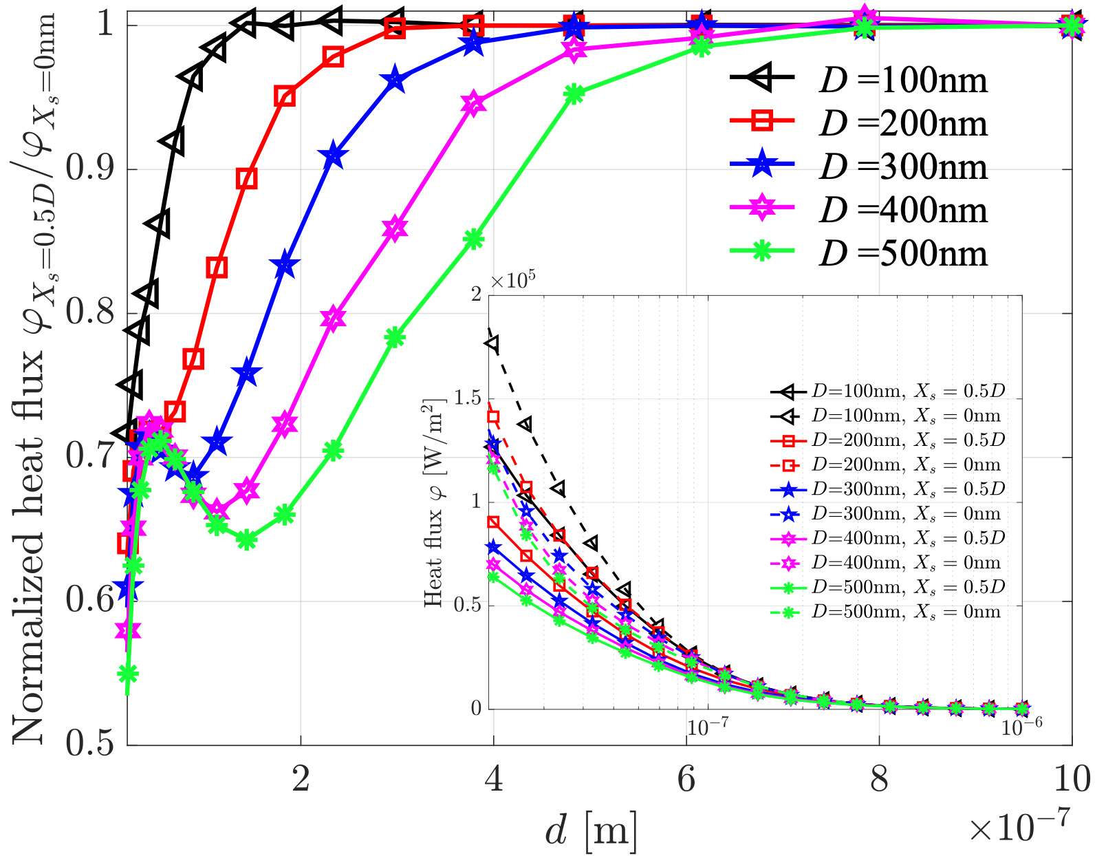
Figure 11: Dependence of the ratio $\varphi_{X_{s}=0.5D}/\varphi_{X_{s}=0\text{nm}}$ (main figure) and the heat flux $\varphi$ (inset) on separation distance $d$ for five different grating periods, $D=100$nm, 200nm, 300nm, 400nm and 500nm. The filling fraction $f$ = 0.5, chemical potential $\mu=0.5$eV.

Although the heat flux $\varphi$ decreases monotonically with the separation $d$ for both $X_{s}=0$nm and $X_{s}=0.5D$, the ratio $\varphi_{X_{s}=0.5D}/\varphi_{X_{s}=0\text{nm}}$ is usually not monotonic with this separation $d$. The dependence of heat flux $\varphi$ on $d$ is not synchronized for the two configurations with lateral shift $X_{s}=0$nm and 0.5$D$. For the gratings with the same filling fraction $f$, as the separation $d$ increases to 200 nm or more, they always have the same heat flux, even though they have different periods $D$. That is, for two gratings with a large enough separation, it is the filling fraction that plays the determining role for the heat transfer, rather than the grating period.

To understand the separation-dependent shift effect on the heat flux, we show its spectrum for two separations ($d=20$nm and 50nm) in Fig. 12. Two relative shifts are considered, $X_{s}=0$nm and $0.5D$ with $D=500$nm, $f$ = 0.5 and $\mu=0.5$eV. The spectra for the configurations of bare slabs and slabs coated with graphene sheets are also added for reference. The graphene coating (including the graphene grating and the graphene sheet) increases the whole heat flux spectrum apart from the peaks. As compared to the graphene grating coating, the graphene sheet coating can induce a reduction of the low-frequency (at around $9\times 10^{13}$rad/s) peak and a redshift of the high-frequency (at around $2\times 10^{14}$rad/s) peak. The lateral shift between the two objects reduces the whole spectrum of heat flux from the dashed blue line to the red solid line (as shown in Fig. 12). The difference between the red line and blue line spectra is more pronounced for small $d$.

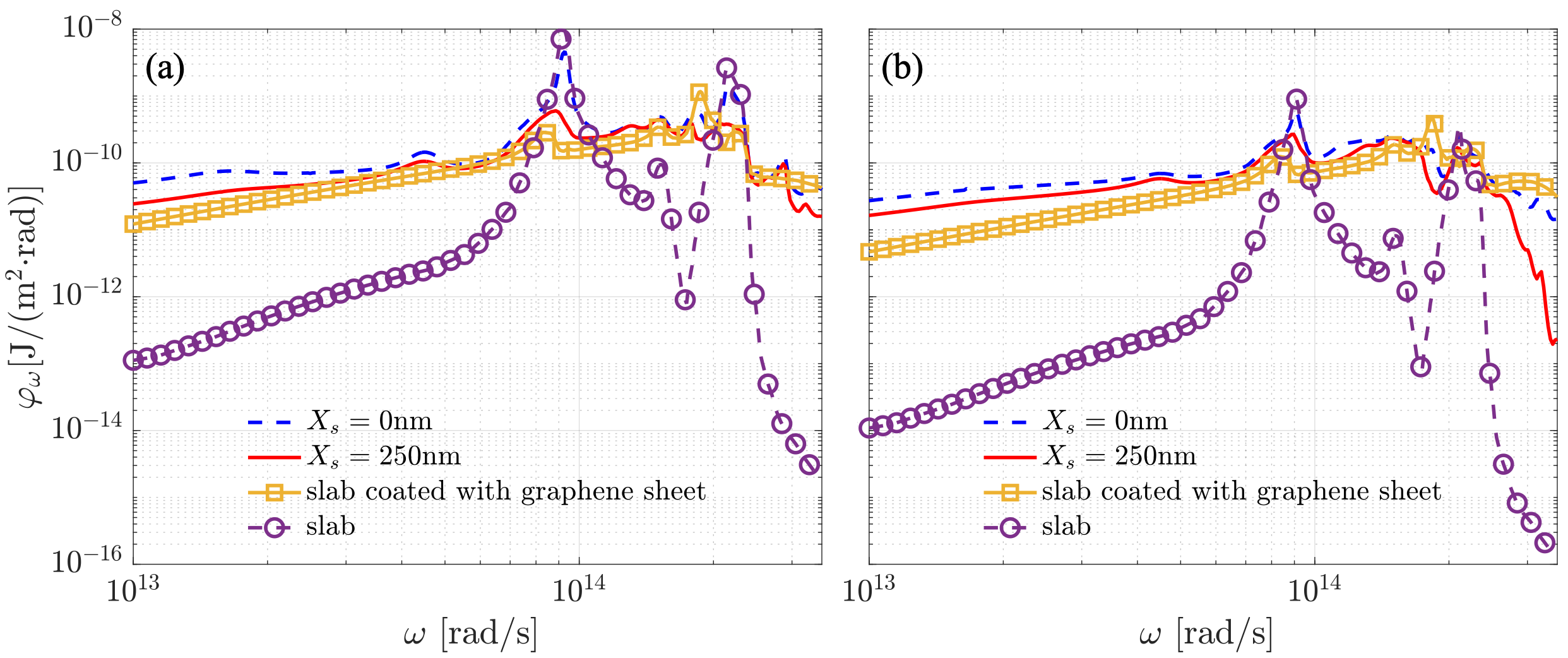
Figure 12: Spectrums of heat flux between two objects with two relative shifts ($X_{s}=0$nm and $0.5D$) and two different separations: (a) separation $d=20$nm, (b) separation $d=50$nm. The grating period $D=500$nm, filling fraction $f$ = 0.5, chemical potential $\mu=0.5$eV. The heat flux spectrums for the configurations of bare slabs and slabs coated with graphene sheets are also added for reference.

To further understand the observations concerning the separation-dependent lateral shift effect on the radiative heat transfer in Figs. 10 and  11, we show the energy transmission coefficient Tr($\mathcal{O}$) (see Eq. (4) for the definition) in the ($k_{x}/k_{0}$, $k_{y}/k_{0}$) plane at the angular frequency $\omega=5\times 10^{13}$rad/s for a slab coated with a graphene grating in Fig. 13. Eight configurations are considered where the upper panels (a-b-c-d) are for the configurations without a lateral shift (i.e., $X_{s}=0$nm), and the lower panels (e-f-g-h) are for configurations with a fixed half-period lateral shift (i.e., $X_{s}=0.5D=250$nm). The separations $d=20$nm, 200nm, 400nm and 600nm are considered while $D=500$nm, $\mu=0.5$eV, and $f$=0.5. The dotted curves represent the dispersion relations obtained from the poles of the reflection coefficient [49, 62].

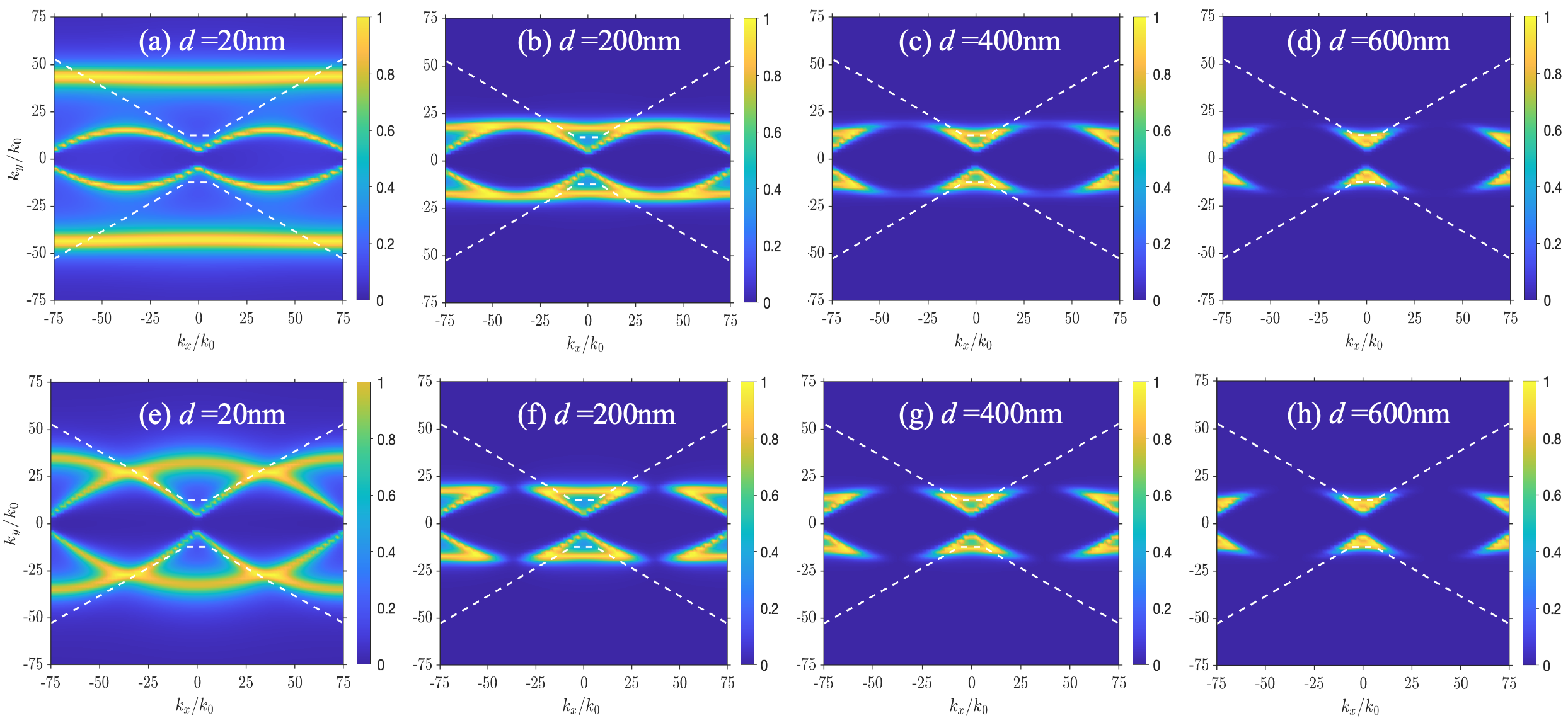
Figure 13: Energy transmission coefficient for a fused silica substrate coated with a graphene grating: (a) separation $d=20$nm and lateral shift $X_{s}=0$nm, (b) separation $d=200$nm and lateral shift $X_{s}=0$nm, (c) separation $d=400$nm and lateral shift $X_{s}=0$nm, (d) separation $d=600$nm and lateral shift $X_{s}=0$nm, (e) separation $d=20$nm and lateral shift $X_{s}=250$nm, (f) separation $d=200$nm and lateral shift $X_{s}=250$nm, (g) separation $d=400$nm and lateral shift $X_{s}=250$nm, (h) separation $d=600$nm and lateral shift $X_{s}=250$nm. The grating period $D=500$nm, chemical potential $\mu=0.5$eV, filling fraction $f$=0.5.

When increasing the separation $d$, by comparing the panels (a-b-c-d) to panels (e-f-g-h) correspondingly in Fig. 13, we show that the difference between the topologies of the allowed modes caused by the relative lateral shift becomes less and less important. In addition, we can see in Fig. 13 a shrinking region for the allowed modes as the separation $d$ increases, regardless of whether there is a lateral shift or not, which results in a decreasing heat flux. Particularly, at separation $d=20$nm, the high-$k$ branch allowed modes blends and hybridizes significantly with the relative low-$k$ branch due to the difference in the near-field caused by the lateral shift. The near-field effect weakens with the mismatch between the two objects. Hence, less energy can be exchanged between the two objects due to the lateral shift at short separation. A general conclusion is that the lateral shift works against the radiative heat transfer for short separations but becomes less important for large separations.

IV conclusion

We analyzed theoretically the effect of a lateral shift on near-field radiative heat transfer between finite-thickness planar fused silica slabs coated with graphene gratings, through an exact Fourier modal method augmented with local basis functions (FMM-LBF). Compared to the effective medium approximation, which treats the grating as an effective whole rather than in detail, this exact approach goes far beyond, especially because the former cannot account for the lateral shift. In order to take into account the lateral shift in the FMM-LBF and besides the existing method of including the lateral shift by directly applying the reference translation to the scattering operators [54], we developed another method to include the lateral shift effect in the scattering operators themselves.

We show that, due to the lateral shift, the heat flux can exhibit significant oscillations and even a 60%-70% reduction compared to the aligned case. Such a lateral shift effect is found to be sensitive to the geometric factor $d/D$. If $d/D<0.5$ (see the Fig. 10 for the regime map of the lateral shift effect), the ratio of the heat flux with a half period shift to that without shift ($\varphi_{X_{s}=0.5D}/\varphi_{X_{s}=0\text{nm}}$) is far from unity. That is, the lateral shift reduces significantly the heat flux. However, we can generally say that when $d/D>2$ the ratio $\varphi_{X_{s}=0.5D}/\varphi_{X_{s}=0\text{nm}}$ approaches unity, where the lateral shift effect on heat transfer becomes less important. We can clearly distinguish two asymptotic regimes for the radiative heat transfer, i.e., the LSE regime and the non-LSE regime, where we see a significant lateral shift effect and a negligible lateral shift effect on heat transfer, respectively.

Regardless of the lateral shift, the radiative heat flux shows a non-monotonic dependence on the graphene chemical potential, with the heat flux reaching its maximum value at $\mu\approx$0.25eV. Considering that all the length scales (e.g., the lateral shift and the period) are realistic and experimentally accessible, the lateral shift sensitive and chemical potential dependent radiative heat transfer might have potential for the thermal logic gate. It would also be interesting to study the effect of the grating’s lateral shift on Casimir interactions [63, 64].

*

Appendix A Modified FMM-LBF with a lateral shift

The main text outlined two distinct approaches to compute the scattering matrix of our structure. In the first approach, the lateral shift is directly incorporated into the scattering matrix elements (as presented in Eq. (8)). In contrast, the second approach requires a modification of the FMM-LBF method itself. This appendix is dedicated to a detailed derivation of the latter approach.

In our recent work [53], we provided comprehensive details of the FMM-LBF with no lateral shift ($X_{s}=0$). In this context, we initially computed the interface scattering matrix $S_{\rm LBF}$ between the input medium I and medium II (as shown in Fig. 2). Then, we determined the slab scattering matrix, denoted $S_{\text{slab}}$, between medium II and medium III. By performing the star product ($\star$) operation [53], between $S_{\rm LBF}$ and $S_{\text{slab}}$, we obtained the overall scattering matrix, denoted $S$ and given by:

$$S=S_{\rm LBF}\star S_{\rm slab}=\begin{pmatrix}\mathcal{R}_{xyz}^{-}&\mathcal{T}_{xyz}^{-}\\ \mathcal{T}_{xyz}^{+}&\mathcal{R}_{xyz}^{+}\end{pmatrix},$$ (9)

where $\mathcal{R}_{xyz}^{+}$ and $\mathcal{R}_{xyz}^{-}$ ($\mathcal{T}_{xyz}^{+}$ and $\mathcal{T}_{xyz}^{-}$) are the reflection operators (transmission operators) in the $(x,y,z)$ Cartesian basis.

In the presence of a lateral shift $X_{s}$, as illustrated in Fig. 2, the definition of the matrix $S_{\rm LBF}$ is modified, while the rest of the calculation process remains the same. Let us proceed to compute this new matrix.

Due to periodicity along the $x$ direction, new diffraction channels open up, characterized by the wave vector component in that direction. The $z$-component of the $n^{\rm th}$ diffraction order wave vector depends on the medium. $k_{zn}^{\rm I}$ and $k_{zn}^{\rm II}$ represent the $z$ wave vector of the $n^{\rm th}$ diffraction order for medium I (with $\varepsilon_{\rm I}$ on the incidence side) and medium II (with $\varepsilon_{\rm II}$ on the output side), respectively, and are given by:

$$\left\{\begin{aligned} k_{zn}^{\rm I}=\sqrt{k_{0}^{2}\varepsilon_{\rm I}-k_{xn}^{2}-k_{y}^{2}},\\ k_{zn}^{\rm II}=\sqrt{k_{0}^{2}\varepsilon_{\rm II}-k_{xn}^{2}-k_{y}^{2}},\end{aligned}\right.$$ (10)

with $k_{0}=\omega/c$, $k_{xn}=k_{x}+n\frac{2\pi}{D}$, $k_{x}$ is in the first Brillouin zone $(-\frac{\pi}{D},\frac{\pi}{D})$, and $k_{y}$ is in $\mathbb{R}$.

The electric field and the magnetic field in medium I can be expressed as

$$\left\{\begin{aligned} \textbf{E}_{\rm I}&=\sum_{n}\left(\textbf{I}_{n}e^{i{\textbf{k}}_{{\rm i}n}\cdot\textbf{r}}+\textbf{R}_{n}e^{i{\textbf{k}}_{{\rm r}n}\cdot\textbf{r}}\right),\\ \textbf{H}_{\rm I}&=\frac{1}{k_{0}Z_{0}}\sum_{n}\left({\textbf{k}}_{{\rm i}n}\times\textbf{I}_{n}e^{i{\textbf{k}}_{{\rm i}n}\cdot\textbf{r}}+{\textbf{k}}_{{\rm r}n}\times\textbf{R}_{n}e^{i{\textbf{k}}_{{\rm r}n}\cdot\textbf{r}}\right),\end{aligned}\right.$$ (11)

Here, $\textbf{I}_{n}=(I_{xn},I_{yn},I_{zn})$, $\textbf{R}_{n}=(R_{xn},R_{yn},R_{zn})$, ${\textbf{k}}_{{\rm i}n}=(k_{xn},k_{y},k_{zn}^{\rm I})$, ${\textbf{k}}_{{\rm r}n}=(k_{xn},k_{y},-k_{zn}^{\rm I})$ and $Z_{0}=\sqrt{\dfrac{\mu_{0}}{\varepsilon_{0}}}$, with $n\in\mathbb{Z}$. Typically, in the numerical implementation, we retain only $2N+1$ Fourier coefficients i.e. $n\in[-N,N]$; where $N$ is called the truncation order.

In medium II, the electric field and the magnetic field are:

$$\left\{\begin{aligned} \textbf{E}_{\rm II}&=\sum_{n}\left(\textbf{T}_{n}e^{i{\textbf{k}}_{{\rm t}n}\cdot\textbf{r}}+\textbf{I}_{n}^{\prime}e^{i{\textbf{k}}_{{\rm i^{\prime}}n}\cdot\textbf{r}}\right),\\ \textbf{H}_{\rm II}&=\frac{1}{k_{0}Z_{0}}\sum_{n}\left({\textbf{k}}_{{\rm t}n}\times\textbf{T}_{n}e^{i{\textbf{k}}_{{\rm t}n}\cdot\textbf{r}}+{\textbf{k}}_{{\rm i^{\prime}}n}\times\textbf{I}_{n}^{\prime}e^{i{\textbf{k}}_{{\rm i^{\prime}}n}\cdot\textbf{r}}\right),\end{aligned}\right.$$ (12)

where $\textbf{T}_{n}=(T_{xn},T_{yn},T_{zn})$, $\textbf{I}_{n}^{\prime}=(I_{xn}^{\prime},I_{yn}^{\prime},I_{zn}^{\prime})$, ${\textbf{k}}_{{\rm t}n}=(k_{xn},k_{y},k_{zn}^{\rm II})$ and ${\textbf{k}}_{{\rm i^{\prime}}n}=(k_{xn},k_{y},-k_{zn}^{\rm II})$.

Furthermore, using ${\rm div}\textbf{E}=\textbf{k}\cdot\textbf{E}=0$, we have the following relations

$$I_{zn}=-\frac{1}{k_{zn}^{\rm I}}(k_{xn}I_{xn}+k_{y}I_{yn}),$$ (13)

$$R_{zn}=\frac{1}{k_{zn}^{\rm I}}(k_{xn}R_{xn}+k_{y}R_{yn}),$$

$$T_{zn}=-\frac{1}{k_{zn}^{\rm II}}(k_{xn}T_{xn}+k_{y}T_{yn}),$$

$$I_{zn}^{\prime}=\frac{1}{k_{zn}^{\rm II}}(k_{xn}I_{xn}^{\prime}+k_{y}I_{yn}^{\prime}).$$

The boundary conditions for the electric field at $z=0$ are

$$\left\{\begin{aligned} E_{{\rm I}x}(x,y,0)=E_{{\rm II}x}(x,y,0),\\ E_{{\rm I}y}(x,y,0)=E_{{\rm II}y}(x,y,0).\end{aligned}\right.$$ (14)

By inserting Eqs. (11) and (12) into Eq. (14), for arbitrary $n$, we have

$$\left\{\begin{aligned} I_{xn}+R_{xn}=I_{xn}^{\prime}+T_{xn},\\ I_{yn}+R_{yn}=I_{yn}^{\prime}+T_{yn},\end{aligned}\right.$$ (15)

which can be expressed in compact form

$$I+R=I^{\prime}+T,$$ (16)

where

$$I=\begin{pmatrix}I_{x}\\ I_{y}\end{pmatrix},R=\begin{pmatrix}R_{x}\\ R_{y}\end{pmatrix},I^{\prime}=\begin{pmatrix}I_{x}^{\prime}\\ I_{y}^{\prime}\end{pmatrix},T=\begin{pmatrix}T_{x}\\ T_{y}\end{pmatrix}.$$ (17)

Due to the zero thickness approximation of the graphene grating, the boundary condition for the magnetic fields at the interface between media I and II are

$$H_{{\rm II}x}(x,y,0)-H_{{\rm I}x}(x,y,0)=\sigma(x)E_{{\rm II}y}(x,y,0),$$ (18)

where the function $\sigma(x)$ is periodic and can be expanded into Fourier series as follows

$$\sigma(x)=\begin{cases}\sigma_{g}&\text{ if }\;\;X_{s}<x<X_{s}+a~{}\textrm{(graphene)}\\ 0&\text{ if }\;\;X_{s}+a<x<X_{s}+D~{}\textrm{(slit)}\end{cases}=\sum_{n}\sigma_{n}e^{i\frac{2\pi}{D}nx}.$$ (19)

By inserting Eqs. (11)and (12) into Eq. (18), and using the Laurent factorization rule, the following relation is obtained

$$\left\{(k_{y}T_{zn}-k_{zn}^{\rm II}T_{yn})+(k_{y}I_{zn}^{\prime}+k_{zn}^{\rm II}I_{yn}^{\prime})\right.$$ (20)

$$\left.-(k_{y}I_{zn}-k_{zn}^{\rm I}I_{yn})-(k_{y}R_{zn}+k_{zn}^{\rm I}R_{yn})\right\}$$

$$=k_{0}Z_{0}\sum_{n^{\prime}}\left\{\sigma_{n^{\prime}-n}(T_{yn^{\prime}}+I_{yn^{\prime}}^{\prime})\right\}.$$

That can be expressed in a compact matrix form as

$$(k_{y}T_{z}-\gamma_{\rm II}T_{y})+(k_{y}I_{z}^{\prime}+\gamma_{\rm II}I_{y}^{\prime})-(k_{y}I_{z}-\gamma_{\rm I}I_{y})$$ (21)

$$-(k_{y}R_{z}+\gamma_{\rm I}R_{y})=k_{0}Z_{0}[[\sigma]](T_{y}+I_{y}^{\prime}),$$

where $\gamma_{\rm II}=$diag($k_{zn}^{\rm II}$), $\gamma_{\rm I}=$diag($k_{zn}^{\rm I}$) and $[[\sigma]]$ is the Toeplitz matrix whose ($n$’, $n$) element is $\sigma_{n^{\prime}-n}$, more precisely:

$$]=\begin{pmatrix}\sigma_{0}&\sigma_{-1}&&&\sigma_{-2N}\\ \sigma_{1}&\sigma_{0}&\sigma_{-1}&&&\\ &\ddots&\ddots&\ddots&\\ &&\ddots&\ddots&\sigma_{-1}&\\ \sigma_{2N}&&&\sigma_{1}&\sigma_{0}&\end{pmatrix},$$ (22)

where $\sigma_{p}$=$\frac{i\sigma_{g}}{2\pi p}e^{-\frac{i2\pi pX_{s}}{D}}\left(e^{-\frac{i2\pi pa}{D}}-1\right)=e^{-\frac{i2\pi pX_{s}}{D}}\overline{\sigma}_{p}$ when $p$ is a non-zero integer, $\sigma_{0}=\sigma_{g}a/D=\overline{\sigma}_{0}$, $\overline{\sigma}_{p}$ and $\overline{\sigma}_{0}$ correspond to the case $X_{s}=0$ [53, 65].

In addition, when considering a lateral translation $X_{s}$, the electric field $E_{x}$ on the graphene grating surface ($z=0$) can be expressed in terms of local basis functions [$g^{\prime}_{m}(x)$ and $s^{\prime}_{m}(x)$] as follows

$$E_{x}(x,y)=e^{ik_{y}y}\left\{\begin{aligned} &\sum_{m=1}^{N_{g}}p_{m}g^{\prime}_{m}(x)\;\;\;\text{if}\;\;X_{s}<x<X_{s}+a\\ &\sum_{m=0}^{N_{s}-1}q_{m}s^{\prime}_{m}(x)\;\;\;\text{if}\;\;X_{s}+a<x<X_{s}+D\\ \end{aligned}\right.,$$ (23)

where

$$\;\;\;\;\;\;\;\;\;\;\;\;\;\;\;\;\;\;\;\;\;\;\;\left\{\begin{aligned} &g_{m}(x)=\sin(m\pi x/a)\\ \\ &s_{m}(x)=\dfrac{\cos(m\pi(x-a)/c^{\prime})}{\sqrt{(c^{\prime}/2)^{2}-(x-x_{c})^{2}}}\end{aligned}\right.,$$ (24)

with $c^{\prime}=D-a$, $x_{c}=(a+D)/2$, $N_{g}={\rm round}\left[\dfrac{N\times a}{D}\right]$, $N_{s}=N-N_{g}$, and round$(x)$ gives the nearest integer number, then

$$\left\{\begin{aligned} &g^{\prime}_{m}(x)=g_{m}(x-X_{s})\;\;{\rm if}~{}~{}X_{s}<x<X_{s}+a\\ \\ &s^{\prime}_{m}(x)=s_{m}(x-X_{s})\;\;{\rm if}~{}~{}X_{s}+a<x<X_{s}+D\end{aligned}\right..$$ (25)

Projecting the boundary condition for the $y$-component of the magnetic field on the $(e^{-ik_{xn}x})$ basis we obtain:

$$(k_{zn}^{\rm II}T_{xn}-k_{xn}T_{zn}-k_{zn}^{\rm II}I_{xn}^{\prime}-k_{xn}I_{zn}^{\prime})$$ (26)

$$-(k_{zn}^{\rm I}I_{xn}-k_{xn}I_{zn}-k_{zn}^{\rm I}R_{xn}-k_{xn}R_{zn})$$

$$=-\sigma_{g}k_{0}Z_{0}\sum_{m=1}^{N_{g}}<e^{-ik_{xn}x},p_{m}g^{\prime}_{m}(x)>,$$

where the scalar product is given by $<f,g>=\frac{1}{D}\int_{X_{s}}^{X_{s}+D}f(x)g(x){\rm d}x$. Then Eq. (26) yields :

$$(k_{zn}^{\rm II}T_{xn}-k_{xn}T_{zn}-k_{zn}^{\rm II}I_{xn}^{\prime}-k_{xn}I_{zn}^{\prime})$$ (27)

$$-(k_{zn}^{\rm I}I_{xn}-k_{xn}I_{zn}-k_{zn}^{\rm I}R_{xn}-k_{xn}R_{zn})$$

$$=-\frac{1}{D}\int_{X_{s}}^{X_{s}+a}\sigma_{g}k_{0}Z_{0}\sum_{m=1}^{N_{g}}p_{m}g_{m}(x-X_{s})e^{-ik_{xn}x}{\rm d}x.$$

Using the change of variable $x^{\prime}=x-X_{s}$, Eq. (27) becomes

$$(k_{zn}^{\rm II}T_{xn}-k_{xn}T_{zn}-k_{zn}^{\rm II}I_{xn}^{\prime}-k_{xn}I_{zn}^{\prime})$$ (28)

$$-(k_{zn}^{\rm I}I_{xn}-k_{xn}I_{zn}-k_{zn}^{\rm I}R_{xn}-k_{xn}R_{zn})$$

$$=-\frac{1}{D}\int_{0}^{a}\sigma_{g}k_{0}Z_{0}\sum_{m=1}^{N_{g}}p_{m}g_{m}(x^{\prime})e^{-ik_{xn}x^{\prime}-ik_{xn}X_{s}}{\rm d}x^{\prime}.$$

By taking out the term $e^{-ik_{xn}X_{s}}$ in the integral and exchanging the order of summation and integration, the RHS of Eq. (28) becomes

$$-\frac{1}{D}\int_{0}^{a}\sigma_{g}k_{0}Z_{0}\sum_{m=1}^{N_{g}}p_{m}g_{m}(x^{\prime})e^{-ik_{xn}x^{\prime}-ik_{xn}X_{s}}{\rm d}x^{\prime}$$ (29)

$$=-\sigma_{g}k_{0}Z_{0}e^{-ik_{xn}X_{s}}\sum_{m=1}^{N_{g}}p_{m}G_{nm},$$

where $G_{nm}=\frac{-ia}{2D}e^{-ik_{xn}a/2}\left[\right.e^{im\pi/2}sinc(\alpha_{nm}^{-}a/2)-$ $e^{-im\pi/2}$ $sinc(\alpha_{nm}^{+}a/2)\left.\right]$, $\alpha_{nm}^{\pm}=m\pi/a\pm k_{xn}$.

Eq. (27) can now be recast in a more compact form :

$$\gamma_{\rm II}T_{x}-\alpha T_{z}-\gamma_{\rm II}I_{x}^{\prime}-\alpha I_{z}^{\prime}-\gamma_{\rm I}I_{x}+\alpha I_{z}$$ (30)

$$+\gamma_{\rm I}R_{x}+\alpha R_{z}=-\sigma_{g}k_{0}Z_{0}\Delta\mathbb{G}p,$$

where $\Delta=\text{diag}(e^{-ik_{xn}X_{s}})$, $\mathbb{G}=\{G_{nm}\}$ is a matrix with size [$(2N+1)\times N_{g}$] and $p$ is the column vector formed by the $N_{g}$ coefficients $p_{m}$ with $p=(p_{1},p_{2},p_{3}\cdots p_{N_{g}})^{\rm T}$. We can write the above equation as follows:

$$\gamma_{\rm II}T_{x}-\alpha T_{z}-\gamma_{\rm II}I_{x}^{\prime}-\alpha I_{z}^{\prime}-\gamma_{1}I_{x}+\alpha I_{z}+\gamma_{1}R_{x}+\alpha R_{z}$$ (31)

$$=-\sigma_{g}k_{0}Z_{0}\left[\Delta\mathbb{G}\;\textbf{0}\right]\begin{pmatrix}p\\ q\end{pmatrix},$$

where $\left[\Delta\mathbb{G}\;\textbf{0}\right]$ is the horizontale concatenation of matrices $\Delta\mathbb{G}$ and the matrix 0 denoting the zero matrix of size [$(2N+1)\times N_{s}$], $q$ is the column vector formed by the $N_{s}$ coefficients $q_{m}$ with $q=(q_{0},q_{1},q_{2}\cdots q_{N_{s}-1})^{\rm T}$.

To obtain $(p,q)^{\rm T}$, we use the boundary condition on the $x$-component of the electric field; and following the same procedure, as that for the $y$-component of the magnetic field, we obtain

$$\begin{pmatrix}p\\ q\end{pmatrix}=\left[\Delta\mathbb{G}\;\Delta\mathbb{S}\right]^{-1}(T_{x}+I_{x}^{\prime}),$$ (32)

where $\left[\Delta\mathbb{G}\;\Delta\mathbb{S}\right]$ is the horizontale concatenation of matrices $\Delta\mathbb{G}$ and $\Delta\mathbb{S}$, $S_{nm}=\frac{\pi}{2D}e^{-ik_{xn}x_{c}}\left[\right.e^{im\pi/2}J_{0}(\beta_{nm}^{-}c^{\prime}/2)+e^{-im\pi/2}J_{0}(\beta_{nm}^{+}c^{\prime}/2)\left.\right]$, $\beta_{nm}^{\pm}=m\pi/c^{\prime}\pm k_{xn}$, $J_{0}(x)$ is the zero-order Bessel function of the first kind.

Finally the modified interface scattering matrix $S_{\rm LBF}$ is given by

$$\begin{pmatrix}R\\ T\end{pmatrix}=S_{\rm LBF}\begin{pmatrix}I\\ I^{\prime}\end{pmatrix},$$ (33)

where

$$S_{\rm LBF}=\begin{pmatrix}\mathbbm{1}&-\mathbbm{1}\\ B&A+\Lambda^{\prime}\end{pmatrix}^{-1}\begin{pmatrix}-\mathbbm{1}&\mathbbm{1}\\ B&A-\Lambda^{\prime}\end{pmatrix},$$ (34)

$\mathbbm{1}$ being the identity matrix of size $[2(2N+1)\times 2(2N+1)]$, $\Lambda^{\prime}={\text{diag}(\sigma k_{0}Z_{0}\left[\mathbb{G}^{\prime}\;0\right]\left[\mathbb{G}^{\prime}\;\mathbb{S}^{\prime}\right]^{-1},[[\sigma]]k_{0}Z_{0})}$, $A$ and $B$ are defined as:

$$A=\begin{pmatrix}\gamma_{\rm II}+\alpha^{2}{\gamma_{\rm II}^{-1}}&{\alpha k_{y}}{\gamma_{\rm II}^{-1}}\\ \\ {\alpha k_{y}}{\gamma_{\rm II}^{-1}}&\gamma_{\rm II}+{k_{y}^{2}}{\gamma_{\rm II}^{-1}}\end{pmatrix},$$ (35)

$$B=\begin{pmatrix}\gamma_{\rm I}+{\alpha^{2}}{\gamma_{\rm I}^{-1}}&{\alpha k_{y}}{\gamma_{\rm I}^{-1}}\\ \\ {\alpha k_{y}}{\gamma_{\rm I}^{-1}}&\gamma_{\rm I}+{k_{y}^{2}}{\gamma_{\rm I}^{-1}}\end{pmatrix}.$$

As mentioned in the beginning of this appendix, the remaining calculations necessary to obtain the scattering matrix of the global structure [i.e. the slab scattering matrix $S_{\rm slab}$ and the transformation matrices from the $(x,y,z)$ Cartesian basis to the (TE, TM) basis] proceed exactly as published in our previous work [53].

References

- Rytov et al. [1989] S. M. Rytov, Y. A. Kravtsov, and V. I. Tatarskii, Priniciples of statistical radiophysics, Vol. 3 (Springer-Verlag, 1989).
- Polder and Van Hove [1971] D. Polder and M. Van Hove, Theory of radiative heat transfer between closely spaced bodies, Phys. Rev. B 4, 3303 (1971).
- Chapuis et al. [2008a] P. O. Chapuis, M. Laroche, S. Volz, and J.-J. Greffet, Near-field induction heating of metallic nanoparticles due to infrared magnetic dipole contribution, Phys. Rev. B 77, 125402 (2008a).
- Narayanaswamy and Chen [2008] A. Narayanaswamy and G. Chen, Thermal near-field radiative transfer between two spheres, Phys. Rev. B 77, 075125 (2008).
- Carminati and Greffet [1999] R. Carminati and J.-J. Greffet, Near-field effects in spatial coherence of thermal sources, Phys. Rev. Lett. 82, 1660 (1999).
- Loomis and Maris [1994] J. J. Loomis and H. J. Maris, Theory of heat transfer by evanescent electromagnetic waves, Phys. Rev. B 50, 18517 (1994).
- Shchegrov et al. [2000] A. V. Shchegrov, K. Joulain, R. Carminati, and J.-J. Greffet, Near-field spectral effects due to electromagnetic surface excitations, Phys. Rev. Lett. 85, 1548 (2000).
- Volokitin and Persson [2001] A. I. Volokitin and B. N. J. Persson, Radiative heat transfer between nanostructures, Phys. Rev. B 63, 205404 (2001).
- Chapuis et al. [2008b] P. O. Chapuis, M. Laroche, S. Volz, and J.-J. Greffet, Radiative heat transfer between metallic nanoparticles, Appl. Phys. Lett. 92, 3303 (2008b).
- Manjavacas and García de Abajo [2012] A. Manjavacas and F. J. García de Abajo, Radiative heat transfer between neighboring particles, Phys. Rev. B 86, 075466 (2012).
- Nikbakht [2018] M. Nikbakht, Radiative heat transfer between core-shell nanoparticles, J. Quant. Spectrosc. Radiat. Transf. 221, 164 (2018).
- Messina et al. [2018] R. Messina, S.-A. Biehs, and P. Ben-Abdallah, Surface-mode-assisted amplification of radiative heat transfer between nanoparticles, Phys. Rev. B 97, 165437 (2018).
- Dong et al. [2018] J. Dong, J. M. Zhao, and L. H. Liu, Long-distance near-field energy transport via propagating surface waves, Phys. Rev. B 97, 075422 (2018).
- Zhang et al. [2019] Y. Zhang, H. L. Yi, H. P. Tan, and M. Antezza, Giant resonant radiative heat transfer between nanoparticles, Phys. Rev. B 100, 134305 (2019).
- Luo et al. [2020a] M. G. Luo, J. M. Zhao, L. H. Liu, and M. Antezza, Radiative heat transfer and radiative thermal energy for two-dimensional nanoparticle ensembles, Phys. Rev. B 102, 024203 (2020a).
- Luo et al. [2023a] M. G. Luo, J. M. Zhao, and L. H. Liu, Heat diffusion in nanoparticle systems via near-field thermal photons, Int. J. Heat Mass Transf. 200, 123544 (2023a).
- Biehs et al. [2011] S.-A. Biehs, F. S. S. Rosa, and P. Ben-Abdallah, Modulation of near-field heat transfer between two gratings, Appl. Phys. Lett. 98, 243102 (2011).
- Kan et al. [2019] Y. H. Kan, C. Y. Zhao, and Z. M. Zhang, Near-field radiative heat transfer in three-body systems with periodic structures, Phys. Rev. B 99, 035433 (2019).
- Liu et al. [2022a] Y. Liu, F. Q. Chen, A. Caratenuto, Y. P. Tian, X. J. Liu, Y. T. Zhao, and Y. Zheng, Effective approximation method for nanogratings-induced near-field radiative heat transfer, Materials 15, 998 (2022a).
- Shen et al. [2009] S. Shen, A. Narayanaswamy, and G. Chen, Surface phonon polaritons mediated energy transfer between nanoscale gaps, Nano Lett. 9, 2909 (2009).
- Rousseau et al. [2009] E. Rousseau, A. Siria, G. Jourdan, S. Volz, F. Comin, J. Chevrier, and J.-J. Greffet, Radiative heat transfer at the nanoscale, Nat. Photonics 3, 514 (2009).
- Ottens et al. [2011] R. S. Ottens, V. Quetschke, S. Wise, A. A. Alemi, R. Lundock, G. Mueller, D. H. Reitze, D. B. Tanner, and B. F. Whiting, Near-field radiative heat transfer between macroscopic planar surfaces, Phys. Rev. Lett. 107, 014301 (2011).
- Song et al. [2015] B. Song, Y. Ganjeh, S. Sadat, D. Thompson, A. Fiorino, V. Fernández-Hurtado, J. Feist, F. J. Garcia-Vidal, J. C. Cuevas, P. Reddy, and E. Meyhofer, Enhancement of near-field radiative heat transfer using polar dielectric thin films, Nat. Nanotechnol. 10, 253 (2015).
- Lim et al. [2015] M. Lim, S. S. Lee, and B. J. Lee, Near-field thermal radiation between doped silicon plates at nanoscale gaps, Phys. Rev. B 91, 195136 (2015).
- Watjen et al. [2016] J. I. Watjen, B. Zhao, and Z. M. Zhang, Near-field radiative heat transfer between doped-si parallel plates separated by a spacing down to 200 nm, Appl. Phys. Lett. 109 (2016).
- Ghashami et al. [2018] M. Ghashami, H. Geng, T. Kim, N. Iacopino, S. K. Cho, and K. Park, Precision measurement of phonon-polaritonic near-field energy transfer between macroscale planar structures under large thermal gradients, Phys. Rev. Lett. 120, 175901 (2018).
- Yang et al. [2018] J. Yang, W. Du, Y. S. Su, et al., Observing of the super-planckian near-field thermal radiation between graphene sheets, Nat. Commun. 9, 4033 (2018).
- DeSutter et al. [2019] J. DeSutter, L. Tang, and M. Francoeur, A near-field radiative heat transfer device, Nat. Nanotechnol. 14, 751 (2019).
- Iqbal et al. [2023] N. Iqbal, S. Zhang, S. Wang, et al., Measuring near-field radiative heat transfer in a graphene- heterostructure, Phys. Rev. Appl. 19, 024019 (2023).
- Yang and Wang [2016] Y. Yang and L. Wang, Spectrally enhancing near-field radiative transfer between metallic gratings by exciting magnetic polaritons in nanometric vacuum gaps, Phys. Rev. Lett. 117, 044301 (2016).
- Messina et al. [2017] R. Messina, A. Noto, B. Guizal, and M. Antezza, Radiative heat transfer between metallic gratings using fourier modal method with adaptive spatial resolution, Phys. Rev. B 95, 125404 (2017).
- Cui et al. [2023] G.-C. Cui, C.-L. Zhou, Y. Zhang, and H.-L. Yi, Significant Enhancement of Near-Field Radiative Heat Transfer by Misaligned Bilayer Heterostructure of Graphene-Covered Gratings, ASME J. Heat Mass Transfer 146, 022801 (2023).
- Svetovoy et al. [2012] V. B. Svetovoy, P. J. van Zwol, and J. Chevrier, Plasmon enhanced near-field radiative heat transfer for graphene covered dielectrics, Phys. Rev. B 85, 155418 (2012).
- Ilic et al. [2012] O. Ilic, M. Jablan, J. D. Joannopoulos, I. Celanovic, H. Buljan, and M. Soljačić, Near-field thermal radiation transfer controlled by plasmons in graphene, Phys. Rev. B 85, 155422 (2012).
- Zheng et al. [2017] Z. H. Zheng, X. L. Liu, A. Wang, and Y. M. Xuan, Graphene-assisted near-field radiative thermal rectifier based on phase transition of vanadium dioxide (VO2), Int. J. Heat Mass Transf. 109, 63 (2017).
- Volokitin [2017] A. Volokitin, Casimir friction and near-field radiative heat transfer in graphene structures, Z. Naturforsch. A 72, 171 (2017).
- Zhao et al. [2017] B. Zhao, B. Guizal, Z. M. Zhang, S. Fan, and M. Antezza, Near-field heat transfer between graphene/hBN multilayers, Phys. Rev. B 95, 245437 (2017).
- Shi et al. [2021] K. Z. Shi, Z. Y. Chen, X. Xu, J. Evans, and S. L. He, Optimized colossal near-field thermal radiation enabled by manipulating coupled plasmon polariton geometry, Advanced Materials 33, 2106097 (2021).
- Liu et al. [2022b] R. Y. Liu, L. X. Ge, H. Y. Yu, Z. Cui, and X. H. Wu, Near-field radiative heat transfer via coupling graphene plasmons with different phonon polaritons in the reststrahlen bands, Eng. Sci. 18, 224 (2022b).
- Lu et al. [2022] L. Lu, B. Zhang, H. Ou, B. W. Li, K. Zhou, J. L. Song, Z. X. Luo, and Q. Cheng, Enhanced near-field radiative heat transfer between graphene/hBN systems, Small 18, 2108032 (2022).
- Wang and Antezza [2023] J.-S. Wang and M. Antezza, Photon mediated energy, linear and angular momentum transport in fullerene and graphene systems beyond local equilibrium (2023), arXiv:2307.11361 .
- Zhang et al. [2022] Y.-M. Zhang, M. Antezza, and J.-S. Wang, Controllable thermal radiation from twisted bilayer graphene, Int. J Heat Mass Transf. 194, 123076 (2022).
- Liu and Zhang [2015] X. L. Liu and Z. M. Zhang, Giant enhancement of nanoscale thermal radiation based on hyperbolic graphene plasmons, Appl. Phys. Lett. 107, 143114 (2015).
- Hu et al. [2020] Y. Z. Hu, H. Li, Y. G. Zhu, and Y. Yang, Enhanced near-field radiative heat transport between graphene metasurfaces with symmetric nanopatterns, Phys. Rev. Appl. 14, 044054 (2020).
- Luo et al. [2023b] M. G. Luo, Y. Jeyar, B. Guizal, J. M. Zhao, and M. Antezza, Effect of graphene grating coating on near-field radiative heat transfer, Appl. Phys. Lett. 123, 253902 (2023b).
- He et al. [2020a] M. J. He, H. Qi, Y. T. Ren, Y. Zhao, and M. Antezza, Active control of near-field radiative heat transfer by a graphene-gratings coating-twisting method, Opt. Lett. 45, 2914 (2020a).
- He et al. [2020b] M. J. He, H. Qi, Y.-T. Ren, Y.-J. Zhao, and M. Antezza, Magnetoplasmonic manipulation of nanoscale thermal radiation using twisted graphene gratings, Int. J. Heat Mass Transf. 150, 119305 (2020b).
- Luo et al. [2020b] M. G. Luo, J. M. Zhao, and M. Antezza, Near-field radiative heat transfer between twisted nanoparticle gratings, Appl. Phys. Lett. 117, 053901 (2020b).
- Zhou et al. [2022a] C.-L. Zhou, Y. Zhang, and H.-L. Yi, Enhancement and manipulation of near-field thermal radiation using hybrid hyperbolic polaritons, Langmuir 38, 7689 (2022a).
- Guizal and Felbacq [1999] B. Guizal and D. Felbacq, Electromagnetic beam diffraction by a finite strip grating, Optics Communications 165, 1 (1999).
- Hwang [2020a] R.-B. Hwang, Highly improved convergence approach incorporating edge conditions for scattering analysis of graphene gratings, Scientific Reports 10, 12855 (2020a).
- Jeyar et al. [2023a] Y. Jeyar, M. Antezza, and B. Guizal, Electromagnetic scattering by a partially graphene-coated dielectric cylinder: Efficient computation and multiple plasmonic resonances, Phys. Rev. E 107, 025306 (2023a).
- Jeyar et al. [2023b] Y. Jeyar, M. G. Luo, K. Austry, B. Guizal, Y. Zheng, H. B. Chan, and M. Antezza, Tunable nonadditivity in the casimir-lifshitz force between graphene gratings, Phys. Rev. A 108, 062811 (2023b).
- Messina and Antezza [2011] R. Messina and M. Antezza, Scattering-matrix approach to casimir-lifshitz force and heat transfer out of thermal equilibrium between arbitrary bodies, Phys. Rev. A 84, 042102 (2011).
- Falkovsky and Varlamov [2007] L. A. Falkovsky and A. A. Varlamov, Space-time dispersion of graphene conductivity, Eur. Phys. J. B 56, 281 (2007).
- Falkovsky [2008] L. A. Falkovsky, Optical properties of graphene, J. Phys. Conf. Ser. 129, 012004 (2008).
- Awan et al. [2016] S. A. Awan, A. Lombardo, A. Colli, G. Privitera, T. S. Kulmala, J. M. Kivioja, M. Koshino, and A. C. Ferrari, Transport conductivity of graphene at RF and microwave frequencies, 2D Mater. 3, 015010 (2016).
- Messina and Antezza [2014] R. Messina and M. Antezza, Three-body radiative heat transfer and casimir-lifshitz force out of thermal equilibrium for arbitrary bodies, Phys. Rev. A 89, 052104 (2014).
- Palik [1998] E. Palik, Handbook of Optical Constants of Solids (Academic, New York, 1998).
- Guérout et al. [2012] R. Guérout, J. Lussange, F. S. S. Rosa, J.-P. Hugonin, D. A. R. Dalvit, J.-J. Greffet, A. Lambrecht, and S. Reynaud, Enhanced radiative heat transfer between nanostructured gold plates, Phys. Rev. B 85, 180301(R) (2012).
- Liu and Zhang [2014] X. L. Liu and Z. M. Zhang, Graphene-assisted near-field radiative heat transfer between corrugated polar materials, Appl. Phys. Lett. 104, 251911 (2014).
- Zhou et al. [2022b] C.-L. Zhou, Y. Zhang, Z. Torbatian, D. Novko, M. Antezza, and H.-L. Yi, Photon tunneling reconstitution in black phosphorus/ heterostructure, Phys. Rev. Mater. 6, 075201 (2022b).
- Noto et al. [2014] A. Noto, R. Messina, B. Guizal, and M. Antezza, Casimir-lifshitz force out of thermal equilibrium between dielectric gratings, Phys. Rev. A 90, 022120 (2014).
- Wang et al. [2021] M. Wang, L. Tang, C. Y. Ng, R. Messina, B. Guizal, J. A. Crosse, M. Antezza, C. T. Chan, and H. B. Chan, Strong geometry dependence of the casimir force between interpenetrated rectangular gratings, Nat. Commun. 12, 600 (2021).
- Hwang [2020b] R.-B. Hwang, Highly improved convergence approach incorporating edge conditions for scattering analysis of graphene gratings, Sci. Rep. 10, 12855 (2020b).