Minimum Covariance Determinant:
Spectral Embedding and Subset Size Determination

Abstract

This paper introduces several ideas to the minimum covariance determinant problem for outlier detection and robust estimation of means and covariances. We leverage the principal component transform to achieve dimension reduction, paving the way for improved analyses. Our best subset selection algorithm strategically combines statistical depth and concentration steps. To ascertain the appropriate subset size and number of principal components, we introduce a novel bootstrap procedure that estimates the instability of the best subset algorithm. The parameter combination exhibiting minimal instability proves ideal for the purposes of outlier detection and robust estimation. Rigorous benchmarking against prominent MCD variants showcases our approach’s superior capability in outlier detection and computational speed in high dimensions. Application to a fruit spectra data set and a cancer genomics data set illustrates our claims.

Keywords: Robustness, Outliers, Principal component analysis, Statistical depth, Bootstrap, Algorithm instability, High-dimensional data

1 Introduction

The minimum covariance determinant (MCD) estimator (Rousseeuw, 1985) and its subsequent extensions have been widely adopted for robust estimation of multivariate location and scatter. This estimator identifies a subset of a predetermined size from multivariate data, aiming for the smallest possible determinant of the sample covariance matrix. MCD rose in popularity after the introduction of a computationally efficient algorithm called fast minimum covariance determinant (FastMCD) (Rousseeuw and Driessen, 1999). FastMCD has found broad applications in finance, econometrics, engineering, the physical sciences, and biomedical research (Hubert et al., 2008, 2018). The minimum covariance determinant estimator is statistically consistent and asymptotically normal (Butler et al., 1993; Cator and Lopuhaä, 2012). It is also an important building block in a variety of robust statistical modelling tasks, including but not limited to principal component analysis (Croux and Haesbroeck, 2000; Hubert et al., 2005), factor analysis (Pison et al., 2003), clustering (Hardin and Rocke, 2004), classification (Hubert and Van Driessen, 2004), and multivariate regression (Rousseeuw et al., 2004). Recent extensions to the minimum covariance determinant paradigm include a kernelized version (Schreurs et al., 2021) for nonelliptical data and a cell-wise version (Raymaekers and Rousseeuw, 2023) for robustness against cell-wise outliers.

The MCD problem can be exactly solved in $O(n\log n)$ arithmetic operations in the univariate case (Rousseeuw and Leroy, 2005). However, computation becomes much more challenging in the multivariate setting. It can be shown that FastMCD is essentially a greedy block minimization algorithm, providing a locally optimal solution for the nonconvex, combinatorial optimization problem of minimizing the sample covariance determinant. Given its greedy nature, the block-descent algorithm can be trapped by local minima. Therefore, proper initialization is crucial, particularly as the proportion of outliers or the dimensionality of the data grows. Naive random initialization falters in these circumstances. Hubert et al. (2012) propose a deterministic initialization strategy called deterministic minimum covariance determinant (DetMCD) that relies on six different initializations for $\mu$ and $\Sigma$. This ensemble strategy can greatly outperform random initialization in robustness and speed when the proportion of outliers is high. However, recent work by Zhang et al. (2023) demonstrates that using the trimmed subset induced by the notion of statistical depth (Zuo and Serfling, 2000) is conceptually simpler, computationally faster, and even more robust.

To its detriment, MCD relies on the computation of Mahalanobis distances, which requires the invertibility of $\hat{\Sigma}$. To tackle the high-dimensional scenario where $p>n$, Boudt et al. (2020) add Tikhonov regularization to the covariance matrix to ensure its positive definiteness. However, their minimum regularized covariance determinant (MRCD) estimator is computationally expensive due to its need to invert large matrices at each iteration. Another direction to achieve high-dimensional outlier detection is to consider alternative definitions of the Mahalanobis distance and study its null asymptotic distribution under suitable model assumptions (Ro et al., 2015; Li and Jin, 2022; Chikun Li and Wu, 2024). This line of work formulates the problem of outlier detection within the framework of hypothesis testing .

This paper explores several new ideas for enhancing and expanding algorithms for the MCD problem. We first propose a best subset selection algorithm based on spectral embedding and statistical depth. The idea of using principle component analysis for dimension reduction in the context of outlier detection has been explored by Hubert et al. (2005), Filzmoser et al. (2008), and Zahariah and Midi (2023). Compared with these approaches, our algorithm is both conceptually and practically simpler. Our second key contribution is the construction of a novel bootstrap procedure for estimating the number of inliers $h$. In the current literature, a principled way to select $h$ is largely absent. Often $h$ is chosen conservatively to ensure the exclusion of every conceivable outlier from the selected subset. Popular choices include $h=\lfloor 0.5n\rfloor$ and $h=\lfloor 0.75n\rfloor$. This practise potentially compromises statistical efficiency. Although various reweighting procedures (Rousseeuw and Driessen, 1999; Hardin and Rocke, 2005; Cerioli, 2010; Ro et al., 2015; Chikun Li and Wu, 2024) may be applied to rescue additional observations as inliers (Rousseeuw and Driessen, 1999), such reweighting prcedures requires the specification of a significance level $\alpha$ that trades off type-I error and power. Moreover, when the model assumptions are not satisfied, the performance of these reweighting procedures may severely deteriorate due to their parametric nature. In a manner akin to clustering instability (Wang, 2010; Fang and Wang, 2012), our bootstrap procedure estimates the instability of our $h$-subset selection algorithm. We find that the subset size exhibiting minimal instability almost always matches the true number of inliers. Thus the estimated $h$ enables us to incorporate as many observations as possible in estimating mean and covariance. Additionally, the selected $h$-subset enables us to discern outliers from inliers in a data-driven, nonparametric manner that is robust to distributional assumptions and eliminates the need for a pre-defined significance level.

2 Background

2.1 Minimum Covariance Determinant

Given a multivariate data matrix $X\in\mathbb{R}^{n\times p}$, assume that most of the observations are sampled from a unimodal distribution with mean $\mu\in\mathbb{R}^{p}$ and covariance $\Sigma\in\mathbb{R}^{p\times p}$. Simultaneously suppose that there exists a subset of outliers markedly diverging from the primary mode. For the purpose of outlier detection and robust estimation, we are interested in finding a subset $H\subset\{1,2,\dots,n\}$ of size $h$ that is outlier-free. The mean and covariance estimated from the subset are given by

$$\begin{split}\hat{\mu}&=\frac{1}{h}\sum_{i\in H}x_{i}\quad\text{and}\quad\hat{\Sigma}=\frac{1}{h}\sum_{i\in H}(x_{i}-\hat{\mu})(x_{i}-\hat{\mu})^{\top},\end{split}$$ (1)

where $x_{i}\in\mathbb{R}^{p}$ is the $i$-th observation in the subset $H$.

Definition 2.1.

The minimum covariance determinant problem seeks the $h$ observations from $x_{1},x_{2},\dots,x_{n}$ minimizing the determinant of $\hat{\Sigma}$ defined in equation (1).

Rousseeuw and Driessen (1999) proposed the first computationally efficient algorithm to tackle the MCD problem named FastMCD. Starting from a random initial subset $H$, FastMCD first obtains an initial estimate of $\mu$ and $\Sigma$ via equation (1). Then, based on the Mahalanobis distances

$$d_{i}=\sqrt{(x_{i}-\hat{\mu})^{\top}\hat{\Sigma}^{-1}(x_{i}-\hat{\mu})},$$ (2)

the observations $x_{i},i=1,2,\dots,n$ are ranked from closest to furthest. Given the rank permutation $\pi$ satisfying $d_{\pi(1)}\leq d_{\pi(2)}\leq\dots\leq d_{\pi(n)}$, $H$ is updated as

$$H=\{\pi(1),\pi(2),\dots,\pi(h)\}.$$ (3)

Rousseeuw and Driessen (1999) call the combination of procedures (1), (2), and (3) a concentration step (C-step). They show that each concentration step monotonically decreases $\det(\hat{\Sigma})$. In the FastMCD algorithm, the concentration step is applied iteratively until the sequence of $\det\hat{\Sigma}$ converges.

2.2 Statistical Depth

Statistical depth is a nonparametric notion commonly used to rank multivariate data from a center outward (Zuo and Serfling, 2000; Zhang et al., 2023). A statistical depth function increases with the centrality of the observation, with values ranging between 0 and 1. After computing the statistical depth of all observations within a data set, it is natural in estimating means and covariances to retain the $h$ observations with the greatest depths. Zhang et al. (2023) investigated the application of two representative depth notions, projection depth and $L_{2}$ depth (Zuo and Serfling, 2000). Their experiments demonstrate that projection depth is more robust across different simulation settings. Projection depth has the added benefit of being affine invariant (Zuo and Serfling, 2000; Zuo, 2006). Therefore, in this work we focus on projection depth as our primary depth notion.

Definition 2.2.

The projection depth of a vector $x\in\mathbb{R}^{p}$ with respect to a distribution $F$ is defined as

$$D(x;F)=\left\{1+\underset{\lVert u\rVert=1}{\sup}\frac{|u^{\top}x-{\rm med}(u^{\top}y)|}{{\rm MAD}(u^{\top}y)}\right\}^{-1},$$ (4)

where $y$ is a multivariate random variable that follows distribution $F$, ${\rm med}(V)$ is the median of a univariate random variable $V$, and ${\rm MAD}(V)={\rm med}(|V-{\rm med}(V)|)$ denotes the median absolute deviation from the median.

Since there exists no closed-form expression for the quantity (4), in practise projection depth is approximated by generating $k$ random directions $u$. For the purpose of ranking the observations from a center outward, one can compute $D(x_{i};\hat{F}_{n})$ for $i$ between $1$ and $n$, where $\hat{F}_{n}$ is the empirical distribution of $X\in\mathbb{R}^{n\times p}$. In this case projection depth is also referred to as sample projection depth. We may write $D(x_{i};\hat{F}_{n})$ as $D(x_{i};X)$ to highlight the dependence on the observed data matrix $X$. Sample projection depths are generally efficient to compute with a time complexity of $O(nkp)$. In the R computing environment, sample projection depths can be computed efficiently via the package ddalpha (Lange et al., 2014; Pokotylo et al., 2016).

2.3 Reweighted Estimators

The fast depth-based (FDB) algorithm of Zhang et al. (2023) consists of three steps: (a) compute statistical depths and define the initial $h$-subset to be the $h$ observations with the largest depths (b) compute $\hat{\mu}$ and $\hat{\Sigma}$ by equation (1), and (c) re-estimate $\hat{\mu}$ and $\hat{\Sigma}$ via the reweighting scheme (5) of Rousseeuw and Driessen (1999).

$$\begin{split}c&=\underset{i}{\text{med}}\quad\frac{\mathcal{D}^{2}(x_{i};\hat{\mu},\hat{\Sigma})}{\chi^{2}_{p,0.5}},\quad w_{i}=\begin{cases}1&\mathcal{D}^{2}(x_{i};\hat{\mu},c\hat{\Sigma})\leq\chi^{2}_{p,0.975}\\ 0&\mathcal{D}^{2}(x_{i};\hat{\mu},c\hat{\Sigma})>\chi^{2}_{p,0.975},\end{cases}\\ \hat{\mu}_{\text{re}}&=\frac{\sum_{i=1}^{n}w_{i}x_{i}}{\sum_{i=1}^{n}w_{i}},\quad\hat{\Sigma}_{\text{re}}=\frac{\sum_{i=1}^{n}w_{i}(x_{i}-\hat{\mu}_{\text{re}})(x_{i}-\hat{\mu}_{\text{re}})^{\top}}{\sum_{i=1}^{n}w_{i}-1}.\end{split}$$ (5)

Here $\mathcal{D}(x_{i};\hat{\mu},\hat{\Sigma})$ is the Mahalanobis distance of $x_{i}$ from the center $\hat{\mu}$. FDB amends the depth-induced $h$-subset to define the optimal subset and skips concentration steps altogether. As we demonstrate in Section 3.3 and Section 5.1, a reweighting procedure like (5) can severely underestimate or overestimate the number of outliers.

3 Methods

3.1 Spectral Embedding

A key ingredient of our methodology is to transform the data to its principal components before best subset selection. The first step in our pipeline is to center the data matrix $X\in\mathbb{R}^{n\times p}$. We then compute the singular value decomposition $\tilde{X}=USV^{T}$ of the centered data $\tilde{X}$, where $V\in\mathbb{R}^{p\times\min\{n,p\}}$. Finally we select the first $q$ principle components $Z=\tilde{X}V[:,1:q]$. The matrix $Z$ is the substrate from which we will identify the best $h$-subset.

Definition 3.1.

Suppose that the first $q$ principle components of $X\in\mathbb{R}^{n\times p}$ is $Z\in\mathbb{R}^{n\times q}$. The spectral minimum covariance determinant problem with parameter $q$ and $h$ is the minimum covariance determinant problem with subset size $h$ defined on $Z$.

As noted in Section 2.2, the time complexity for computing sample projection depths for a data set of size $n\times p$ is $O(nkp)$. Spectral embedding automatically alleviates the computational burden in estimating projection depth by reducing the number of columns from $p$ to $q$, the number of principal components. Spectral embedding may also reduce the required number of random directions $k$. The artificial “point” outlier data of (Hubert et al., 2012; Zhang et al., 2023) illustrates the virtues of operating on principal components. Section 4.1 outlines the data generation protocol for these data. The data matrix $X$ is $400\times 40$, with 25% of the observations replaced by outliers. Figure 1 depicts the decline in the outlier count in the $h=300$ retained observations as a function of $k$ and $q$. As expected, with rising $k$, the $h$-subset includes fewer outliers. Employing only 2 or 10 principal components results in a notably faster decline in the average number of outliers compared to employing all 40 principal components. The left panel of Figure 1 suggests that the first two principal components already capture the inlier/outlier structure. The remaining components carry redundant information, obscuring projection depth approximation. Because projection depth is affine invariant, using all 40 principal components for computing projection depths is equivalent to using the original data matrix $X$.

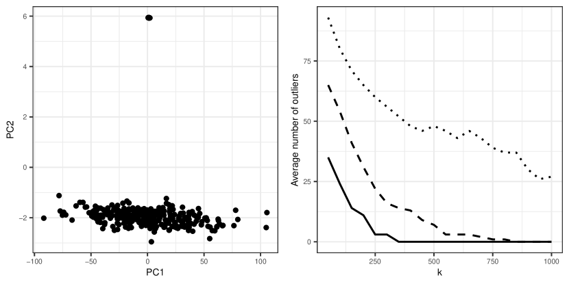
Figure 1: The left panel shows the distribution of the first and second principle components. The right panel shows the average number of outliers included in the $h$-subset induced by projection depths over 100 random replicates. Solid line shows counts for $q=2$, dashed line shows counts for $q=10$, dotted line shows counts for $q=40$.

3.2 Concentration Steps

When the specified subset size $h$ is close to the true number of inliers and projection depth is difficult to approximate, Figure 1 shows that depth-induced $h$-subsets may still contain several outliers. The FDB algorithm of Zhang et al. (2023), which skips concentration steps, is able to work well despite possible outliers in the $h$-subset because the reweighting step (5) adds an additional layer of projection. Unfortunately, we demonstrate in Section 3.3 and Section 5.1 that the reweighting step (5) itself may be detrimental to outlier detection. Moreover, when $p>n$, the reweighting step is stymied by the singularity of the matrix $\hat{\Sigma}$. To ensure that the identified $h$-subset contains as few outliers as possible, we may employ concentration steps as described in Section 2.1 to further refine the $h$-subset. Algorithm 1 summarizes our best $h$-subset selection algorithm.

Algorithm 1 Spectral Minimum Covariance Determinant (SpectralMCD)

0:  Data matrix $X\in\mathbb{R}^{n\times p}$, subset size $h<n$, number of principle components $q\leq\min\{n,p\}$, number of random directions $k$.

1:  Center $X$ to obtain $\tilde{X}$ and compute the singular value decomposition $\tilde{X}=USV^{T}$.

2:  Compute the principle components matrix $Z=\tilde{X}V[:,1:q]$ and the projection depths $d_{i}=D(z_{i};Z),i=1,2,\dots,n$, using $k$ random directions.

3:  Sort $d_{i}$ in decreasing order, yielding permutation $\pi$ with $d_{\pi(1)}\geq d_{\pi(2)}\geq\dots\geq d_{\pi(n)}$. Set $H=\{\pi(1),\pi(2),\dots,\pi(h)\}$.

4:  Update $H$ using regular concentration steps (1), (2), (3) on the principle component matrix $Z$ until $H$ stabilizes.

4:  The best $h$-subset $H$.

3.3 Estimating the Number of Outliers

In the MCD literature, choosing the right subset size $h$ has remained a persistent challenge. In our methodology, while spectral embedding brings numerous advantages, determining the optimal number of principal components introduces another hurdle. Drawing inspiration from the notion of clustering instability (Wang, 2010; Fang and Wang, 2012), in this section describe a bootstrap procedure for estimating the number of inliers $h$ (or the number of outliers $n-h$), as well as the appropriate number of principle components $q$. The task of robust location/scatter estimation may be considered as a special case of clustering with two clusters, where one cluster consists of inliers, and the other cluster consists of outliers. Contrary to traditional clustering, the outlier cluster does not necessarily exhibit spatial structure. This causes classic strategies in clustering such as the gap statistic (Tibshirani et al., 2001) to fail. We propose to use projection depth to distinguish outliers from inliers, given an identified $h$-subset. If $h$ is suitably chosen, then different bootstrapped samples should yield similar conclusions about which observations are outliers in the original data matrix. To this end, we first define a distance between two binary mappings (0 represents inlier, 1 represents outlier).

Definition 3.2.

The clustering distance between the binary mappings $\psi_{1}$ and $\psi_{2}$ with respect to distribution $F$ is defined as

$$d_{F}(\psi_{1},\psi_{2})=E_{x\sim F,y\sim F}\{|I_{\psi_{1}(x)=\psi_{1}(y)}-I_{\psi_{2}(x)=\psi_{2}(y)}|\}.$$

Through applying the outlier detection algorithm to a pair of independent bootstrap samples $\dot{X}$ and $\ddot{X}$, we can construct two binary mappings $\psi(\dot{X},h,q)$ and $\psi(\ddot{X},h,q)$.

Definition 3.3.

The instability of the outlier detection algorithm $\psi$ (with parameter $h$ and $q$) is defined as

$$s(\psi,h,q)=E_{\dot{X},\ddot{X}}[d_{\hat{F}_{n}}\{\psi(\dot{X},h,q),\psi(\ddot{X},h,q)\}],$$

where each row of $\dot{X}$ and $\ddot{X}$ are independently sampled from $\hat{F}_{n}$.

In practise, for a bootstrap pair $\dot{X}_{b}$ and $\ddot{X}_{b}$, $d_{\hat{F}_{n}}\{\psi(\dot{X}_{b},h,q),\psi(\ddot{X}_{b},h,q)\}$ is estimated as

$$\hat{d}_{\hat{F}_{n}}\{\psi(\dot{X}_{b},h,q),\psi(\ddot{X}_{b},h,q)\}=\frac{1}{n^{2}}\sum_{i=1}^{n}\sum_{j=1}^{n}|I_{\psi_{1}(x_{i})=\psi_{1}(x_{j})}-I_{\psi_{2}(x_{i})=\psi_{2}(x_{j})}|,$$ (6)

where $\psi_{1}(x)=\{\psi(\dot{X}_{b},h,q)\}(x)$, $\psi_{2}(x)=\{\psi(\ddot{X}_{b},h,q)\}(x)$. Equation (6) is the standard definition of clustering distance. However, it has been demonstrated that this definition of clustering dissimilarity heavily depends on the cluster sizes (Haslbeck and Wulff, 2020). In our context, it becomes problematic when $h$ approaches $n$, in which case there is very little room for two binary mappings to disagree. For example, in the extreme scenario of $h=n$, all observations will always be mapped to 0 and (6) will always be 0. To adjust for the effect of cluster sizes, Haslbeck and Wulff (2020) give a corrected definition of clustering distance, namely

$$\hat{d}^{c}_{\hat{F}_{n}}\{\psi(\dot{X}_{b},h,q),\psi(\ddot{X}_{b},h,q)\}=\frac{\hat{d}_{\hat{F}_{n}}\{\psi(\dot{X}_{b},h,q),\psi(\ddot{X}_{b},h,q)\}}{2c(1-c)}-1,$$ (7)

where $c=\{{h\choose 2}+{n-h\choose 2}\}/{n\choose 2}$ is the expectation of $I_{\psi_{1}(x)=\psi_{1}(y)}$. The statistic (7) estimates $\text{corr}(I_{\psi_{1}(x)=\psi_{1}(y)},1-I_{\psi_{2}(x)=\psi_{2}(y)})$ as opposed to Definition 3.2. Due to the limitation of space, we direct readers to Haslbeck and Wulff (2020) for the detailed derivation of (7).

Using the corrected version of clustering distance, the (corrected) instability of our outlier detection algorithm is estimated as

$$\hat{s}^{c}(\psi,h,q)=\frac{1}{B}\sum_{b=1}^{B}\hat{d}^{c}_{\hat{F}_{n}}\{\psi(\dot{X}_{b},h,q),\psi(\ddot{X}_{b},h,q)\},$$ (8)

where we average over $B$ independent bootstrap pairs.

Algorithm 2 provides the details of our instability estimation algorithm. In practise, we search over a pre-set collection of pairs $(h,q)$ to identify a parameter combination with minimal instability. Although Algorithm 2 appears computationally intensive at first glance, many computational results can be recycled during a grid search. Specifically, we only need to compute the singular value decomposition and principle component projection once for each bootstrap sample. For $q$ fixed, the computed projection depths can be used for all values of $h$. We can also skip the concentration steps in Algorithm 1 since a few outliers in the identified $h$-subset do not tangibly affect the binary mappings derived from projection depths. These practical considerations make the algorithm much more efficient.

Algorithm 2 Instability Estimation

0:  Data matrix $X\in\mathbb{R}^{n\times p}$, subset size $h<n$, number of principle components $q\leq\min\{n,p\}$, number of random directions $k$, number of bootstrap pairs $B$.

1:  for $b=1:B$ do

2:     Construct a pair of bootstrapped samples $\dot{X}_{b}$ and $\ddot{X}_{b}$.

3:     Apply Algorithm 1 to $\dot{X}_{b}$ and $\ddot{X}_{b}$ to obtain best $h$-subsets $\dot{H}_{b}$ and $\ddot{H}_{b}$. As by products, store the column means $\dot{\mu}_{b}$ and $\ddot{\mu}_{b}$ of $\dot{X}_{b}$ and $\ddot{X}_{b}$, the right singular matrices $\dot{V}_{b}$ and $\ddot{V}_{b}$, and the principle components $\dot{Z}_{b}$ and $\ddot{Z}_{b}$.

4:     Center and right multiply $X$ with $(\dot{\mu}_{b},\dot{V}_{b}[:,1:q])$ and $(\ddot{\mu}_{b},\ddot{V}_{b}[:,1:q])$ respectively to obtain $\dot{Z}$ and $\ddot{Z}$.

5:     Compute projection depths $\dot{d}_{i}=D(\dot{z}_{i};\dot{Z}_{b}[\dot{H}_{b},]),\ddot{d}_{i}=D(\ddot{z}_{i};\ddot{Z}_{b}[\ddot{H}_{b},]),i=1,2,\dots,n$ with $k$ random directions.

6:     Set $\psi_{1}(x_{i})=0$ if $\dot{d}_{i}$ is within the $h$-largest and $\psi_{1}(x_{i})=1$ otherwise. $\psi_{2}(x_{i})$ is defined similarly.

7:     Compute $\hat{d}^{c}_{\hat{F}_{n}}\{\psi(\dot{X}_{b},h,q),\psi(\ddot{X}_{b},h,q)\}$ by equation (7).

8:  end for

8:  $\hat{s}^{c}(\psi,h,q)$ defined in (8).

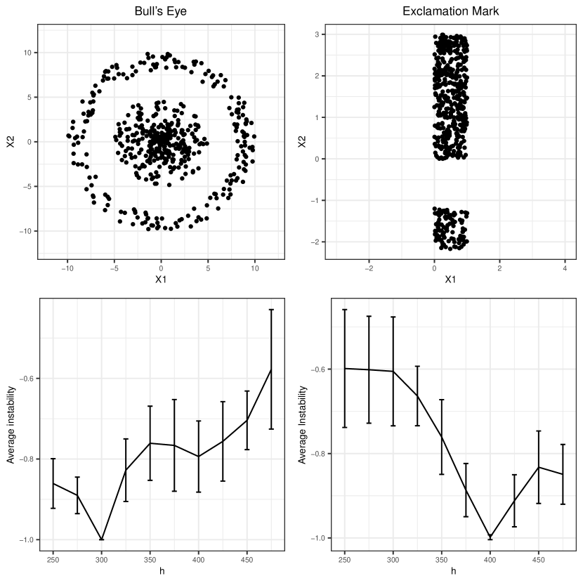
Figure 2: Top left panel is the generated example bull’s eye. Bottom left panel is its instability path averaged over 50 bootstrap pairs, error bar denotes $\pm 1$ standard deviation. Top right panel is the generated example exclamation mark. Bottom right panel is its instability path.

Figure 2 demonstrates the power of Algorithm 2 in two examples, “Bull’s Eye” and “Exclamation Mark”, with 500 observations and 2 features each. “Bull’s Eye” has 200 points in the outer rim, while “Exclamation Mark” has 100 points in the bottom rectangle. We set $q=2$ and apply Algorithm 2 over the grid $h=250,275,\dots,475$. As Figure 2 shows, Algorithm 2 is able to correctly identify the number of observations in the dominant mode in both cases. We also examined how many observations the FDB algorithm (Zhang et al., 2023) designates as outliers. Here a point is categorized as an outlier if $w_{i}=0$ in the reweighting step (5). Despite having a perfectly specified $h$, FDB estimates 62 outliers in the bull’s eye example and 64 outliers in the exclamation mark example, both of which are underestimations. This failure is likely due to the arbitrary cut-off value 0.975 in the reweighting step (5), which may not be universally suitable.

4 Simulation Studies

4.1 The Overdetermined Case $n>p$

In this section, we evaluate our methods under the simulation protocol employed by both DetMCD (Hubert et al., 2012) and FDB (Zhang et al., 2023). The common simulation protocol first generates inliers as $x_{i}=Gy_{i}$, where $y_{i}$ is Gaussian $\mathcal{N}(0,I_{p})$. The $p\times p$ matrix $G$ has diagonal elements equal to 1 and off-diagonal elements equal to 0.75. The protocol then generates potential outliers at contamination levels of 10%, 25%, and 40%. The outliers are categorized into four types: (a) Point outliers $y_{i}\sim\mathcal{N}(ra\sqrt{p},0.01^{2}I_{p})$, where $a$ is a unit vector orthogonal to $1=(1,1,\dots,1)^{\top}$, (b) Cluster outliers $y_{i}\sim\mathcal{N}(rp^{-1/4}1,I_{p})$, (c) Random outliers $y_{i}\sim\mathcal{N}(rp^{1/4}\nu_{i}/\lVert\nu_{i}\rVert,I_{p})$, where $\nu_{i}\sim\mathcal{N}(0,I_{p})$, and (d) Radial outliers $y_{i}\sim\mathcal{N}(0,5I_{p})$. The scalar $r$ determines the separation of the inlier and outlier clusters. We use $r=5$ throughout this section. Point, Cluster, and Radial outliers were introduced by Hubert et al. (2012) and Random outliers by Zhang et al. (2023).

We omit comparison with DetMCD since in Zhang et al. (2023), their experiments demonstrate that FDB performs almost uniformly better than DetMCD. For FDB, we assume no prior knowledge of the number of outliers and conservatively equate $h$ to $\lfloor 0.5n\rfloor$, the breakdown point for MCD estimators. For spectral MCD, we employ the following pipeline: (a) apply Algorithm 2 to search over the grid $h=\lfloor 0.5n\rfloor,\lfloor 0.55n\rfloor,\dots,\lfloor 0.95n\rfloor$ and $q=2,p$ to pinpoint the parameter combination $(\hat{h},\hat{q})$ with the least average instability, (b) identify the optimal $h$-subset via Algorithm 1 based on $(h,q)=(\hat{h},\hat{q})$, and (c) estimate $\mu_{X}$ and $\Sigma_{X}$ by the formulas (1). Unless stated to the contrary, we set the number of random directions $k=\max\{1000,10q\}$. The outlier types Random and Radial seem to need a larger number of random directions for Algorithm 2 to work properly. Therefore, in these two scenarios we set $k=\max\{1000,30q\}$ to approximate projection depths accurately. The estimators for the data set $Y$ are then obtained as $\hat{\mu}_{Y}=G^{-1}\hat{\mu}_{X}$ and $\hat{\Sigma}_{Y}=G^{-1}\hat{\Sigma}_{X}G^{-1}$.

Our evaluation of the quality of these estimators relies on the following measures:

• $e_{\mu}=\lVert\hat{\mu}_{Y}-\mu_{Y}\rVert_{2}$, where $\mu_{Y}$ is the true mean vector of $Y$ (in this case $\mu_{Y}=0$).

• $e_{\Sigma}=\log_{10}\{\text{cond}(\hat{\Sigma}_{Y}\Sigma_{Y}^{-1})\}$, where $\Sigma_{Y}$ is the true covariance matrix of $Y$ (in this case $\Sigma_{Y}=I_{p}$) and the operator cond finds the condition number of a matrix.

• The Kullback–Leibler divergence

  $$\text{KL}(\hat{\Sigma}_{Y},\Sigma_{Y})=\text{tr}(\hat{\Sigma}_{Y}\Sigma_{Y}^{-1})-\log\{\det(\hat{\Sigma}_{Y}\Sigma_{Y}^{-1})\}-p,$$ (9)

  where the trace operator tr equals the sum of the diagonal entries of a matrix.

We consider three combinations of $n$ and $p$: $(n,p)=(400,40)$, $(n,p)=(400,80)$, and $(n,p)=(2000,200)$. Table 1 and Table 2 list results for the combination $(n,p)=(400,40)$ and $(n,p)=(400,80)$; the results for $(n,p)=(2000,200)$ and statistics on computation time appear in Appendix A.

Table 1: Simulation results when $(n,p)=(400,40)$. All measures are averaged over 50 random replicates. The numbers in parentheses are standard errors. Abbreviations are KL: Kullback–Leibler divergence, FDB: fast depth-based method algorithm, and Spec: spectral minimum covariance determinant.

Outlier	Metric	10%		25%		40%
		FDB	Spec	FDB	Spec	FDB	Spec
Point	$e_{\mu}$	0.346 (0.035)	0.320 (0.030)	0.379 (0.044)	0.366 (0.045)	25.30 (0.100)	1.358 (3.881)
	$e_{\Sigma}$	0.629 (0.031)	0.567 (0.023)	0.659 (0.032)	0.623 (0.027)	6.113 (0.244)	0.903 (0.693)
	KL	2.870 (0.163)	2.375 (0.096)	3.148 (0.191)	2.826 (0.153)	231.1 (2.744)	18.54 (58.79)
Cluster	$e_{\mu}$	0.351 (0.037)	0.328 (0.034)	0.369 (0.035)	0.355 (0.037)	0.405 (0.040)	0.400 (0.038)
	$e_{\Sigma}$	0.624 (0.032)	0.566 (0.026)	0.658 (0.036)	0.619 (0.025)	0.722 (0.029)	0.712 (0.027)
	KL	2.843 (0.177)	2.383 (0.107)	3.180 (0.187)	2.864 (0.137)	3.753 (0.189)	3.631 (0.193)
Random	$e_{\mu}$	0.358 (0.039)	0.336 (0.035)	0.380 (0.043)	0.366 (0.043)	0.407 (0.050)	0.400 (0.051)
	$e_{\Sigma}$	0.624 (0.027)	0.558 (0.024)	0.658 (0.026)	0.621 (0.024)	0.711 (0.028)	0.698 (0.025)
	KL	2.853 (0.169)	2.358 (0.108)	3.177 (0.155)	2.878 (0.134)	3.732 (0.175)	3.597 (0.155)
Radial	$e_{\mu}$	0.354 (0.039)	0.328 (0.034)	0.369 (0.039)	0.355 (0.037)	0.407 (0.040)	0.401 (0.038)
	$e_{\Sigma}$	0.624 (0.032)	0.566 (0.026)	0.656 (0.030)	0.619 (0.025)	0.723 (0.026)	0.711 (0.027)
	KL	2.837 (0.174)	2.383 (0.107)	3.184 (0.187)	2.864 (0.137)	3.748 (0.189)	3.632 (0.193)

Table 2: Simulation results for $(n,p)=(400,80)$. All measures are averaged over 50 random replicates. KL, Kullback–Leibler divergence. Abbreviations are KL: Kullback–Leibler divergence, FDB: fast depth-based algorithm, and Spec: spectral minimum covariance determinant.

Outlier	Metric	10%		25%		40%
		FDB	Spec	FDB	Spec	FDB	Spec
Point	$e_{\mu}$	0.575 (0.049)	0.469 (0.037)	0.605 (0.048)	0.522 (0.045)	35.52 (1.320)	3.057 (7.715)
	$e_{\Sigma}$	1.125 (0.039)	0.855 (0.027)	1.161 (0.038)	0.956 (0.028)	7.122 (0.334)	1.555 (1.424)
	KL	15.98 (0.784)	9.771 (0.262)	16.79 (0.727)	11.91 (0.254)	679.9 (23.96)	68.03 (158.7)
Cluster	$e_{\mu}$	0.579 (0.053)	0.465 (0.039)	0.610 (0.052)	0.518 (0.043)	0.621 (0.053)	0.585 (0.045)
	$e_{\Sigma}$	1.138 (0.043)	0.856 (0.022)	1.165 (0.039)	0.958 (0.025)	1.201 (0.038)	1.100 (0.034)
	KL	16.22 (0.760)	9.776 (0.248)	16.75 (0.716)	11.97 (0.304)	17.70 (0.574)	15.39 (0.389)
Random	$e_{\mu}$	0.582 (0.053)	0.467 (0.037)	0.601 (0.051)	0.519 (0.036)	0.607 (0.052)	0.572 (0.052)
	$e_{\Sigma}$	1.143 (0.037)	0.862 (0.022)	1.173 (0.044)	0.952 (0.028)	1.215 (0.038)	1.109 (0.038)
	KL	16.11 (0.619)	9.770 (0.213)	16.92 (0.658)	11.94 (0.302)	18.02 (0.593)	15.58 (0.680)
Radial	$e_{\mu}$	0.586 (0.054)	0.465 (0.039)	0.594 (0.054)	0.518 (0.043)	0.627 (0.050)	0.585 (0.045)
	$e_{\Sigma}$	1.143 (0.043)	0.856 (0.022)	1.167 (0.05)	0.958 (0.025)	1.215 (0.043)	1.110 (0.034)
	KL	16.42 (0.852)	9.776 (0.248)	16.82 (0.852)	11.97 (0.304)	18.07 (0.579)	15.39 (0.389)

Table 1 and Table 2 shows that our pipeline consistently offers more precise estimates than FDB, particularly in estimating $\Sigma$. The advantage of spectral MCD becomes more pronounced as the proportion of outliers decreases, since it tries to incorporate as many observations as possible. As $p$ goes from 40 to 80, we see that the performance of FDB deteriorates, and the comparative advantage of spectral MCD becomes more evident. This might be due to the fact that the reweighting step (5) becomes less reliable as $p$ grows. Additionally, it is evident that Algorithm 2 effectively selected the appropriate $h$ across nearly all scenarios, except for the Point outliers scenario at a 40% outlier level. In this particular setting, both methods struggle to identify numerous outliers, and estimations is fraught with significant errors. We speculate that this specific setting is statistically impossible for MCD estimators. The Random scenario with outlier proportion 40% is the only other scenario where Algorithm 2 does not perfectly select the true number of inliers. In this case Algorithm 2 selects $h=\lfloor 0.55n\rfloor$ half of the time. Finally, it is worth noting that while our pipeline yields more accurate estimates, it does so at the expense of a computationally intensive bootstrap procedure and takes considerably longer to run than the two baseline methods. Consult Table 4 in Appendix A for specific timing comparisons.

4.2 The Underdetermined Case $p>n$

In this section, we compare our method to minimum regularized covariance determinant (MRCD) (Boudt et al., 2020) and FDB (Zhang et al., 2023) in the high-dimensional case where $p$ is possibly greater than $n$. In this setting the sample covariance matrix is singular, and FDB’s reweighting step must be skipped. We adopt the simulation protocol of Boudt et al. (2020), but extend $p$ beyond the range previously considered. Without loss of generality, we set the mean vector $\mu\in\mathbb{R}^{p}$ to $0$. The covariance matrix $\Sigma$ is constructed iteratively to ensure that its condition number (CN) closely approximates $50$. Section 4 of (Agostinelli et al., 2015) explains in detail this covariance matrix generation protocol. Our simulated outliers are generated from the distribution $\mathcal{N}(50a,\Sigma)$, where $a$ is the unit eigenvector corresponding to the smallest eigenvalue of $\Sigma$. This specific setup is intentionally crafted so that the direction defined by $a$ poses the greatest difficulty in outlier detection.

As in Section 4.1, we put $h=\lfloor 0.5n\rfloor$ for the two baseline methods. We first apply Algorithm 2 to search over the grid $h=\lfloor 0.5n\rfloor$, $\lfloor 0.55n\rfloor$,$\dots$,$\lfloor 0.95n\rfloor$ and $q=2,10,100$. To its credit, Algorithm 2 consistently selects the correct $h$ and $q=2$ for each replicate across all values of $p$. Subsequently, we apply Algorithm 1 to identify the outliers at the optimal parameter combination. For all three methods, once the $h$-subset is obtained, we follow Boudt et al. (2020) in computing the final estimate

$$\hat{\Sigma}{\rho}=\rho I+(1-\rho)\hat{\Sigma}_{H},$$ (10)

where $\hat{\Sigma}_{H}$ represents the usually singular sample covariance matrix based on the subset $H$. The parameter $\rho$ is determined so that $\hat{\Sigma}_{\rho}$ has the desired condition number $CN$. Forcing the generated positive definite covariance matrices to have a common condition number places the three algorithms on an equal footing for comparison.

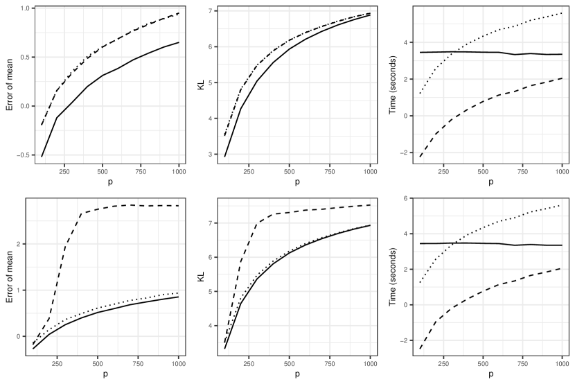
Figure 3: Experimental results for high-dimensional data. First and second row corresponds to outlier level 10% and 40%, respectively. Data points are averaged over 20 replicates. The y-axis for all panels are transformed to log scale for better visualization. Solid line is for spectral MCD, dashed line is for FDB, dotted line is for MRCD.

We evaluate the statistical precision of the three methods using the metrics $e_{\mu}$ and Kullback–Leibler divergence defined in Section 4.1. Additionally, we measure total elapsed time to assess computational efficiency. For our method, the total elapsed time includes the time required for the grid search to identify the optimal parameter combination. Fixing $n$ at 300, we vary $p$ over the range $100,200,\dots,1000$.

Figure 3 depicts the experimental results. Our pipeline consistently offers better statistical precision than the two baseline methods by incorporating more observations. The computation time of MRCD appears to scale cubically with $p$, while the computation time of our workflow (including grid search) remains almost constant. As a result, when $p$ grows sufficiently large, our workflow becomes more efficient than minimum regularized covariance determinant, even though we invoke a costly bootstrap procedure to search for the best parameter combination. In general, FDB is lightning quick compared to the other two methods. However, when the outlier proportion reaches $40\%$, it unfortunately breaks down and yields large estimation errors. Although our workflow is also based on projection depth, it remains robust in this setting. This again highlights the virtue of using the principle component transform to reveal the hidden low-dimensional structure of the data.

5 Real Data Examples

5.1 Fruit Data

Our first real data example, referred to as the fruit data, comprises spectra from three distinct cantaloupe cultivars, labeled D, M, and HA with corresponding sample sizes of 490, 106, and 500. Originally introduced by Hubert and Van Driessen (2004) and later examined by Hubert et al. (2012), this data set encompasses $1096$ total observations recorded across 256 wavelengths. Hubert and Van Driessen (2004) note that the cultivar HA encompasses three distinct groups derived from various illumination systems. However, we have no knowledge of the assignment of individual observations to specific subgroups and the potential impact of the subgroups on spectra.

Our purpose is to estimate the number of outliers and decide which observations qualify as outliers. FDB with $h=\lfloor 0.5n\rfloor$ is our the baseline method. As in Section 3.3, an observation $x_{i}$ is flagged by FDB as an outlier when $w_{i}$ in the reweighting step (5) equals 0. For our method, we initially conduct a grid search using 50 bootstrap pairs and Algorithm 2 over the grid $h=\lfloor 0.5n\rfloor,\lfloor 0.55n\rfloor,\dots,\lfloor 0.95n\rfloor$ at $q=2$. The grid search took 276 seconds to complete. We the use Algorithm 1 to identify the inliers and outliers using the optimal parameter combination. The choice of $q=2$ is motivated by a scree plot analysis where nearly all variance can be explained using just two principal components (Hubert et al., 2012).

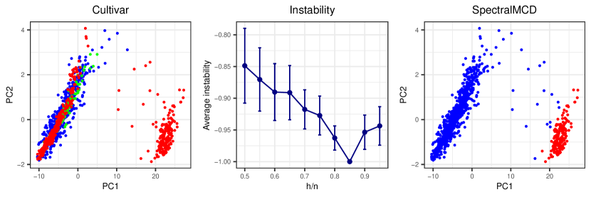
Figure 4: Experimental results for the fruit data set. In the left panel, blue points are of cultivar D, green points are of cultivar M, red points are of cultivar HA. In the right panel, blue points are inliers while red points are outliers.

Figure 4 depicts the experimental outcomes. The left panel of Figure 4 shows the first two principal components of the data set, with each point colored by the corresponding cultivar. Evidently, observations significantly diverging from the primary mode almost exclusively belong to the HA cultivar. The middle panel displays the instability path computed by Algorithm 2, which is minimized at $h=\lfloor 0.85n\rfloor$. The right panels illustrate the assignment of inliers and outliers identified by SpectralMCD using the parameter combination $(h=\lfloor 0.85n\rfloor,q=2)$. SpectralMCD appears quite effective in segregating the two modes, although there are a few points far away from the primary mode that are not assigned as outliers. This might be due to the fact that our search grid is not fine grained enough. FDB in this example categorizes 497 points as outliers using a cut-off of 0.975, which is hard to interpret given the principle component visualization. We suspect that the reweighting procedure (5) might have failed due to the ill conditioning of the estimated covariance matrix. Algorithm 2 estimates approximately $1096*0.15\approx 164$ outliers, roughly a third of the 500 observations. We conjecture that the outliers in the HA cultivar correspond to a subgroup with a distinctive illumination pattern.

5.2 Breast Cancer Data

Our second real data example comes from the The Cancer Genome Atlas (TCGA) project (Network, 2012). The breast cancer project (TCGA-BRCA) contains data on approximately 1100 patients with invasive carcinoma of the breast. Our data is sourced from cBioPortal (Cerami et al., 2012). We focus on the mRNA expression profiles of the patients. These profiles represent expression levels for 20531 genes on the 1100 samples. After performing a $\log_{2}(x+1)$ transform on the expression levels, we retained the top 2000 most variable genes. Apart from expression profiles, the data also record the estrogen receptor (ER) status of each sample. Women with estrogen receptor negative status (ER-) are typically diagnosed at a younger age and have a higher mortality rate (Bauer et al., 2007). Out of 1100 samples, 812 are estrogen receptor positive, 238 are negative, 48 are indeterminate, and 2 are missing. We retain the 1050 samples for which the estrogen receptor status is either positive or negative. Thus, our preprocessed data matrix has dimension $1050\times 2000$.

As in Section 5.1, we first applied Algorithm 2 to estimate the proportion of outliers in the data set. Unlike the fruit data set, a scree plot for these data reveals a wider spread of the variance across many principle components. Therefore, we searched via Algorithm 2 over a two-dimensional parameter grid $q=2,10,100$ and $h=\lfloor 0.5n\rfloor,\lfloor 0.55n\rfloor,\dots,\lfloor 0.95n\rfloor$. The grid search takes 1182 seconds to complete. We then applied Algorithm 1 to identify the outliers under this optimal parameter combination.

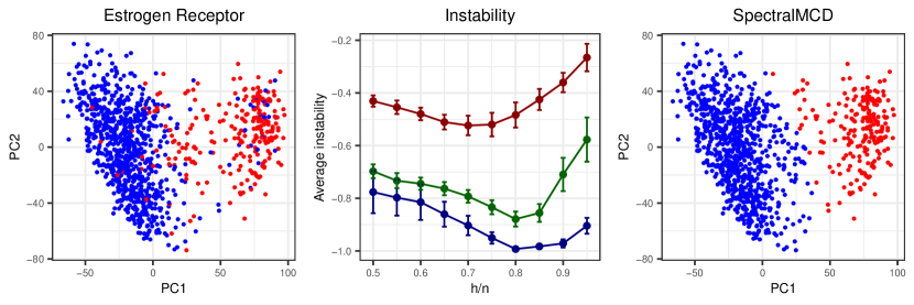
Figure 5: Experimental results for the breast cancer data set. In the left panel, blue points are estrogen receptor positive, red points are negative. In the middle panel, blue, green, red lines are instability paths at $q=2$, $q=10$, $q=100$. In the right panel, blue points are inliers while red points are outliers.

Figure 5 depicts the experimental results. At $q=2$ and $10$, the instability is minimized at $h=\lfloor 0.8n\rfloor$. However, at $q=100$, the instability is minimized at $h=\lfloor 0.7n\rfloor$. Possibly the redundant principle components obscure the inlier/outlier structure. To minimize algorithmic instability, we select the optimal parameter combination $(h,q)=(\lfloor 0.8n\rfloor,2)$. In the general population, about 79-84% of breast cancer cases will be estrogen receptor positive (Allison et al., 2020). Our algorithms are able to infer this medical fact purely from the gene expression profile without reference to recorded estrogen receptor status. Moreover, if we consider this problem as a binary classification problem, Algorithm 1 achieves an unsupervised classification accuracy of 92.4%.

Acknowledgement

We thank Seyoon Ko and Do Hyun Kim for useful suggestions.

Appendix A Additional Simulation Results

Table 3: Simulation results for $(n,p)=(2000,200)$. All measures are averaged over 50 random replicates. Abbreviations are KL: Kullback–Leibler divergence, FDB: fast depth-based method, and Spec: spectral minimum covariance determinant.

Outlier	Metric	10%		25%		40%
		FDB	Spec	FDB	Spec	FDB	Spec
Point	$e_{\mu}$	0.369 (0.015)	0.338 (0.009)	0.389 (0.014)	0.365 (0.016)	56.30 (1.944)	9.748 (19.71)
	$e_{\Sigma}$	0.663 (0.008)	0.589 (0.006)	0.706 (0.010)	0.650 (0.010)	6.932 (0.375)	1.613 (1.836)
	KL	14.57 (0.258)	11.65 (0.156)	16.20 (0.225)	14.03 (0.132)	1157 (21.15)	265.2 (522.0)
Cluster	$e_{\mu}$	0.372 (0.017)	0.337 (0.014)	0.388 (0.019)	0.360 (0.018)	0.414 (0.017)	0.406 (0.016)
	$e_{\Sigma}$	0.665 (0.011)	0.589 (0.008)	0.703 (0.011)	0.649 (0.011)	0.756 (0.007)	0.734 (0.007)
	KL	14.57 (0.191)	11.61 (0.100)	16.14 (0.203)	14.02 (0.152)	18.69 (0.180)	17.80 (0.141)
Random	$e_{\mu}$	0.364 (0.019)	0.326 (0.014)	0.386 (0.014)	0.360 (0.013)	0.411 (0.030)	0.401 (0.031)
	$e_{\Sigma}$	0.661 (0.011)	0.583 (0.008)	0.700 (0.009)	0.647 (0.009)	0.761 (0.010)	0.738 (0.009)
	KL	14.54 (0.247)	11.61 (0.054)	17.79 (0.527)	16.12 (0.217)	18.67 (0.277)	17.73 (0.329)
Radial	$e_{\mu}$	0.371 (0.022)	0.337 (0.014)	0.387 (0.018)	0.360 (0.018)	0.414 (0.018)	0.406 (0.016)
	$e_{\Sigma}$	0.665 (0.011)	0.587 (0.008)	0.704 (0.011)	0.649 (0.011)	0.756 (0.009)	0.735 (0.007)
	KL	14.58 (0.247)	11.61 (0.010)	16.22 (0.199)	11.97 (0.304)	18.83 (0.185)	17.80 (0.141)

Table 4: Computation time averaged over 50 random replicates. Abbreviations are FDB: fast depth-based method, and Spec: spectral minimum covariance determinant.

Outlier	Combination	10%		25%		40%
		FDB	Spec	FDB	Spec	FDB	Spec
Point	(400,40)	0.021	24.19	0.025	23.63	0.022	24.39
	(400,80)	0.092	31.40	0.062	27.79	0.074	31.70
	(2000,200)	2.382	574.1	2.478	607.3	2.391	605.7
Cluster	(400,40)	0.019	23.80	0.019	21.80	0.020	21.95
	(400,80)	0.066	32.60	0.064	29.47	0.073	31.35
	(2000,200)	2.029	521.7	2.128	559.6	1.981	513.6
Random	(400,40)	0.020	26.19	0.021	26.14	0.018	24.28
	(400,80)	0.086	72.74	0.081	59.13	0.069	56.38
	(2000,200)	2.301	1769	2.267	1680	1.929	1474
Radial	(400,40)	0.020	26.42	0.019	24.01	0.022	31.31
	(400,80)	0.068	55.57	0.083	58.18	0.070	57.00
	(2000,200)	2.194	1588	2.400	1751	2.059	1620

Appendix B Miscellaneous

B.1 Exact Solution for Univariate Minimum Covariance Determinant

It is discussed in Hubert and Debruyne (2010) that the univariate minimum covariance determinant problem can be solved in $O(n\log n)$ operations by considering contiguous windows of $h$-subsets. However, somewhat surprisingly, we could not find a detailed exposition of the specific procedure in the literature. In this section we provide a detailed description of the univariate algorithm and prove that it indeed finds the optimal solution. In the univariate case, minimum covariance determinant recduces to finding $h<n$ observations among $x_{1},x_{2},\dots,x_{n}$ with minimal sample variance. One first sorts $x_{1},x_{2},\dots,x_{n}$ and then slides a window of length $h$ along the the sorted array. At each position of the window, the sample mean and sample variance are updated and the sample variance is recorded. A best subset minimizes the $n-h$ recorded sample variances. More specifically, suppose that the order statistics are denoted as $y_{1}\leq y_{2}\leq\dots\leq y_{n}$. The first window consists of observations $y_{1},y_{2},\dots,y_{h}$, with sample mean and variance

$$\mu_{h}=\frac{1}{h}\sum_{i=1}^{h}y_{i}\quad\text{and}\quad\sigma^{2}_{h}=\frac{1}{h}\sum_{i=1}^{h}(y_{i}-\mu_{h})^{2}.$$

As we move the window to the right one position, we may employ Welford’s formula (Welford, 1962) to update these two statistics via

$$\mu_{h+1} =\frac{1}{h+1}(h\mu_{h}+y_{h+1}),$$

$$\sigma^{2}_{h+1} =\frac{h}{h+1}\sigma^{2}_{h}+\frac{1}{h}(y_{h+1}-\mu_{h+1})^{2},$$

$$\mu_{h} =\frac{1}{h}\left[(h+1)\mu_{h+1}-y_{1}\right],$$

$$\sigma^{2}_{h} =\frac{h+1}{h}\sigma^{2}_{h+1}-\frac{h+1}{h^{2}}(y_{1}-\mu_{h+1})^{2}$$

at a cost of $O(1)$. The updated sample variance is added to our list. We repeat this process until the reaching the last window with right endpoint $y_{n}$. Tracking the minimal $\sigma^{2}_{h}$ encountered as well as its corresponding starting and ending positions solves the problem at a cost of $O(n\log n)$, which is dominated by sorting.

To convince readers that this algorithm finds the optimal $h$-subset, we argue by contradiction. Consider a subset $S$ that possesses the lowest subset variance. Within $S$, let $l$ and $u$ represent the smallest and largest numbers, respectively. Now suppose we select any number $x$ from the entire sample such that $l<x<u$, but $x$ is not included in the subset $S$. Let us substitute $x$ for $l$ if $x\leq\bar{x}_{S}$ and for $u$ if $x>\bar{x}_{S}$. This results in a new subset, which we denote as $T$. We clearly have

$$\sum_{i\in T}(x_{i}-\bar{x}_{T})^{2}\leq\sum_{i\in T}(x_{i}-\bar{x}_{S})^{2}<\sum_{i\in S}(x_{i}-\bar{x}_{S})^{2},$$

which contradicts the assumption that $S$ is the subset with the lowest variance. Thus, any observation that falls between $(l,u)$ must also fall in the subset. In other words, the optimal subset must occupy a contiguous window among the order statistics.

B.2 Efficient Computation for FastMCD

The main computational bottleneck for the classic fast minimum covariance determinant algorithm, or simply concentration steps, is the evaluating the matrix inversion $\Sigma^{-1}$ and the determinant $\det\Sigma$. In this section we describe a computational technique that enables us to only perform the matrix inversion and determinant evaluation at the first iteration. In the following iterations, $\Sigma^{-1}$ and $\det\Sigma$ can be updated using the Sherman-Morrison formula and matrix discriminant lemma.

Notice that in the multivariate setting, the Welford updates and downdates of the sample mean $\mu$ and the sample covariance matrix $\Sigma$ become

$$\mu_{h+1} = \frac{1}{h+1}(h\mu_{h}+y_{h+1})$$

$$\mu_{h} = \frac{1}{h}\Big{[}(h+1)\mu_{h+1}-y_{h+1}\Big{]}$$

$$\Sigma_{h+1} = \frac{h}{h+1}\Sigma_{h}+\frac{1}{h}(y_{h+1}-\mu_{h+1})(y_{h+1}-\mu_{h+1})^{\top}$$

$$\Sigma_{h} = \frac{h+1}{h}\Sigma_{h+1}-\frac{h+1}{h^{2}}(y_{h+1}-\mu_{h+1})(y_{h+1}-\mu_{h+1})^{\top}.$$

Given that the update and downdate of $\Sigma$ are rank-1 perturbations of $\Sigma$, we can invoke the Sherman-Morrison formula

$$(A+uv^{\top})^{-1}=A^{-1}-\frac{A^{-1}uv^{\top}A^{-1}}{1+v^{\top}A^{-1}u},$$

to update and downdate $\Sigma^{-1}$. We may also invoke the the matrix determinant lemma

$$\det(A+uv^{\top})=\det A(1+v^{\top}A^{-1}u)$$

to update and downdate $\det\Sigma$.

More specifically, we can update $\Sigma_{h+1}^{-1}$ and $\det\Sigma_{h+1}^{-1}$ as

$$\Sigma_{h+1}^{-1} = (\frac{h+1}{h}\Sigma^{-1}_{h})-\frac{(\frac{h+1}{h}\Sigma^{-1}_{h})(y_{h+1}-\mu_{h+1})(y_{h+1}-\mu_{h+1})^{\top}(\frac{h+1}{h}\Sigma^{-1}_{h})}{h+(y_{h+1}-\mu_{h+1})^{\top}(\frac{h+1}{h}\Sigma^{-1}_{h})(y_{h+1}-\mu_{h+1})}$$

$$\det\Sigma_{h+1} = \frac{h}{h+1}\det\Sigma_{h}(1+\frac{1}{h}(y_{h+1}-\mu_{h+1})^{\top}(\frac{h+1}{h}\Sigma^{-1}_{h})(y_{h+1}-\mu_{h+1})).$$

The downdate to $\Sigma_{h}^{-1}$ and $\det\Sigma_{h}^{-1}$ can be performed similarly, but we omit it here for brevity. At each concentration step, some new observations are included into the $h$-subset, while a same number of old observations are removed from the $h$-subset. We will need to perform an update for each new observation in the $h$-subset and a downdate for each removed observation.

References

- Agostinelli et al. (2015) Agostinelli, C., Leung, A., Yohai, V. J., and Zamar, R. H. (2015), “Robust estimation of multivariate location and scatter in the presence of cellwise and casewise contamination,” Test, 24, 441–461.
- Allison et al. (2020) Allison, K. H., Hammond, M. E. H., Dowsett, M., McKernin, S. E., Carey, L. A., Fitzgibbons, P. L., Hayes, D. F., Lakhani, S. R., Chavez-MacGregor, M., Perlmutter, J., Perou, C. M., Regan, M. M., Rimm, D. L., Symmans, W. F., Torlakovic, E. E., Varella, L., Viale, G., Weisberg, T. F., McShane, L. M., and Wolff, A. C. (2020), “Estrogen and Progesterone Receptor Testing in Breast Cancer: ASCO/CAP Guideline Update,” Journal of Clinical Oncology, 38, 1346–1366, pMID: 31928404.
- Bauer et al. (2007) Bauer, K. R., Brown, M., Cress, R. D., Parise, C. A., and Caggiano, V. (2007), “Descriptive analysis of estrogen receptor (ER)-negative, progesterone receptor (PR)-negative, and HER2-negative invasive breast cancer, the so-called triple-negative phenotype,” Cancer, 109, 1721–1728.
- Boudt et al. (2020) Boudt, K., Rousseeuw, P. J., Vanduffel, S., and Verdonck, T. (2020), “The minimum regularized covariance determinant estimator,” Statistics and Computing, 30, 113–128.
- Butler et al. (1993) Butler, R., Davies, P., and Jhun, M. (1993), “Asymptotics for the minimum covariance determinant estimator,” The Annals of Statistics, 1385–1400.
- Cator and Lopuhaä (2012) Cator, E. A. and Lopuhaä, H. P. (2012), “Central limit theorem and influence function for the MCD estimators at general multivariate distributions,” Bernoulli, 18, 520 – 551.
- Cerami et al. (2012) Cerami, E., Gao, J., Dogrusoz, U., Gross, B. E., Sumer, S. O., Aksoy, B. A., Jacobsen, A., Byrne, C. J., Heuer, M. L., Larsson, E., Antipin, Y., Reva, B., Goldberg, A. P., Sander, C., and Schultz, N. (2012), “The cBio Cancer Genomics Portal: An Open Platform for Exploring Multidimensional Cancer Genomics Data,” Cancer Discovery, 2, 401–404.
- Cerioli (2010) Cerioli, A. (2010), “Multivariate outlier detection with high-breakdown estimators,” Journal of the American Statistical Association, 105, 147–156.
- Chikun Li and Wu (2024) Chikun Li, B. J. and Wu, Y. (2024), “Outlier detection via a minimum ridge covariance determinant estimator,” .
- Croux and Haesbroeck (2000) Croux, C. and Haesbroeck, G. (2000), “Principal component analysis based on robust estimators of the covariance or correlation matrix: influence functions and efficiencies,” Biometrika, 87, 603–618.
- Fang and Wang (2012) Fang, Y. and Wang, J. (2012), “Selection of the number of clusters via the bootstrap method,” Computational Statistics & Data Analysis, 56, 468–477.
- Filzmoser et al. (2008) Filzmoser, P., Maronna, R., and Werner, M. (2008), “Outlier identification in high dimensions,” Computational statistics & data analysis, 52, 1694–1711.
- Hardin and Rocke (2004) Hardin, J. and Rocke, D. M. (2004), “Outlier detection in the multiple cluster setting using the minimum covariance determinant estimator,” Computational Statistics & Data Analysis, 44, 625–638.
- Hardin and Rocke (2005) — (2005), “The distribution of robust distances,” Journal of Computational and Graphical Statistics, 14, 928–946.
- Haslbeck and Wulff (2020) Haslbeck, J. M. and Wulff, D. U. (2020), “Estimating the number of clusters via a corrected clustering instability,” Computational Statistics, 35, 1879–1894.
- Hubert and Debruyne (2010) Hubert, M. and Debruyne, M. (2010), “Minimum covariance determinant,” Wiley interdisciplinary reviews: Computational statistics, 2, 36–43.
- Hubert et al. (2018) Hubert, M., Debruyne, M., and Rousseeuw, P. J. (2018), “Minimum covariance determinant and extensions,” Wiley Interdisciplinary Reviews: Computational Statistics, 10, e1421.
- Hubert et al. (2008) Hubert, M., Rousseeuw, P. J., and Aelst, S. V. (2008), “High-Breakdown Robust Multivariate Methods,” Statistical Science, 23, 92 – 119.
- Hubert et al. (2005) Hubert, M., Rousseeuw, P. J., and Vanden Branden, K. (2005), “ROBPCA: a new approach to robust principal component analysis,” Technometrics, 47, 64–79.
- Hubert et al. (2012) Hubert, M., Rousseeuw, P. J., and Verdonck, T. (2012), “A deterministic algorithm for robust location and scatter,” Journal of Computational and Graphical Statistics, 21, 618–637.
- Hubert and Van Driessen (2004) Hubert, M. and Van Driessen, K. (2004), “Fast and robust discriminant analysis,” Computational Statistics & Data Analysis, 45, 301–320.
- Lange et al. (2014) Lange, T., Mosler, K., and Mozharovskyi, P. (2014), “Fast nonparametric classification based on data depth,” Statistical Papers, 55, 49–69.
- Li and Jin (2022) Li, C. and Jin, B. (2022), “Outlier Detection via a Block Diagonal Product Estimator,” Journal of Systems Science and Complexity, 35, 1929–1943.
- Network (2012) Network, T. C. G. A. (2012), “Comprehensive molecular portraits of human breast tumours,” Nature, 490, 61–70.
- Pison et al. (2003) Pison, G., Rousseeuw, P. J., Filzmoser, P., and Croux, C. (2003), “Robust factor analysis,” Journal of Multivariate Analysis, 84, 145–172.
- Pokotylo et al. (2016) Pokotylo, O., Mozharovskyi, P., and Dyckerhoff, R. (2016), “Depth and depth-based classification with R-package ddalpha,” arXiv preprint arXiv:1608.04109.
- Raymaekers and Rousseeuw (2023) Raymaekers, J. and Rousseeuw, P. J. (2023), “The cellwise minimum covariance determinant estimator,” Journal of the American Statistical Association, just–accepted.
- Ro et al. (2015) Ro, K., Zou, C., Wang, Z., and Yin, G. (2015), “Outlier detection for high-dimensional data,” Biometrika, 102, 589–599.
- Rousseeuw (1985) Rousseeuw, P. J. (1985), “Multivariate estimation with high breakdown point,” Mathematical statistics and applications, 8, 37.