Chern numbers in two-dimensional systems with spiral boundary conditions

Abstract

We discuss methods for calculating Chern numbers of two-dimensional lattice systems using spiral boundary conditions, which sweep all lattice sites in one-dimensional order. Specifically, we establish the one-dimensional representation of Fukui-Hatsugai-Suzuki’s method, based on lattice gauge theory, and the Coh-Vanderbilt’s method, which relates to electronic polarization. The essential point of this discussion is that the insertion of flux into the extended one-dimensional chain generates an effective current in the perpendicular direction. These methods are valuable not only for a unified understanding of topological physics in different dimensions but also for numerical calculations, including the density matrix renormalization group.

I Introduction

For over a decade, there has been extensive research on topological phases and transitions in the context of topological insulators [1, 2, 3, 4, 5, 6, 7]. Topological insulators exhibit energy gaps in the bulk and gapless edge (surface) states in two (three) dimensions. The concept of topology has been further extended to include topological superconductors, Kitaev systems, non-Hermitian skin effects, and other related phenomena [8, 9, 10].

On the other hand, the study of topological phases and transitions in one-dimensional (1D) quantum spin systems has been ongoing since the 1970s. For instance, the dimer-Néel transition in a spin-$1/2$ frustrated anisotropic Heisenberg chain and the successive dimerization observed in Haldane gap systems are interpreted as transitions between different gapped phases that possess distinct topological properties [11, 12, 13, 14].

In this paper, we present a unified study of topological phases and transitions in various systems and dimensions using the concept of electronic polarization and related concepts [15, 16, 17, 18]. In 1D lattice electron systems, we introduce polarization operator (or twist operator) $U$ defined as the exponential of the position operator, and consider its expectation value in the ground state $\ket{\Psi_{0}}$:

$$z=\braket{\Psi_{0}}{U}{\Psi_{0}},\quad U=\exp\biggl{(}{\rm i}\frac{2\pi}{L}\sum_{j=1}^{L}jn_{j}\biggr{)}.$$ (1)

Here, $L$ represents the number of sites, $n_{j}$ is the electron number operator at the $j$-th site. Resta established a relationship between $z$ and electronic polarization, given by $\lim_{L\to\infty}(e/2\pi){\rm Im}\;\!\ln z$ [16]. The signs of $z$ provide information about the system’s topology, such as the presence of charge or spin density waves and edge states [19, 20]. Furthermore, the condition $z=0$ can be utilized to detect phase transition points.

The same quantity as in Eq. (1) was also introduced in the Lieb-Schultz-Mattis (LSM) theorem for 1D quantum systems [21, 22, 23, 24, 25]. In the LSM theorem, Eq. (1) appears as an overlap between the ground state and a variational excited state. According to the theorem, an energy gap above non-degenerate ground state is possible for $z\neq 0$ with $L\to\infty$.

Thus the property of $z$ has been well studied for 1D systems. However, its application to higher-dimensional systems is not fully discussed. In our preceeding work [26], we have extended the twist operator in Eq. (1) to two-dimensional (2D) systems using spiral boundary conditions (SBCs) that encompass all lattice sites in one-dimensional order as illustrated in Fig. 1. These boundary conditions have been utilized to extend the LSM theorem to higher dimensions [27, 28, 29], eliminating unphysical limitations on the system size [30]. By calculating $z$ with SBCs, we have examined the 2D Wilson-Dirac model [31, 32] and identified topological transition points as $z=0$.

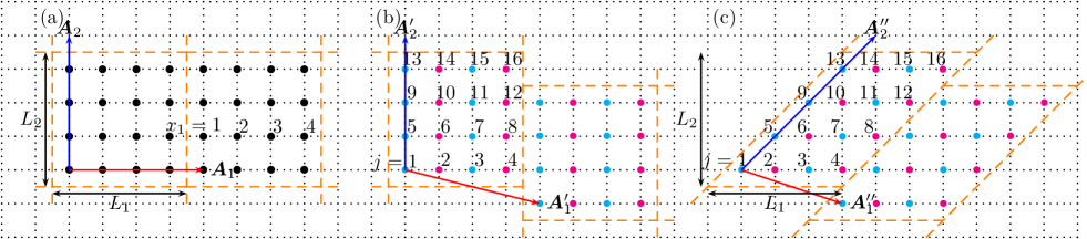
Figure 1: Several boundary conditions for 2D square lattices with $L_{1}\times L_{2}$ sites: (a) Conventional periodic boundary conditions (PBCs), (b) Spiral boundary conditions (SBCs) for $(\pi,0)$ charge order, and (c) SBCs for $(\pi,\pi)$ order. For the systems with SBCs, the lattices are labeled as extended 1D chains.

However, the aforementioned extension does not account for transverse response, so that it does not include the information of the Chern number. Therefore, $z$ needs to be modified to incorporate the flux effect, which is perpendicular to the twist direction. For conventional periodic boundary conditions (PBCs), this extension was carried out by Coh and Vanderbilt for the Haldane model [33]. On the other hand, Fukui, Hatsugai, and Suzuki proposed a method to calculate the Chern number based on the lattice gauge theory [34]. Therefore, we aim to elucidate the relationship between the Coh-Vanderbilt’s method and the Fukui-Hatsugai-Suzuki’s method. Subsequently, we derive the formalism of electronic polarization with SBCs to identify the system’s topology by Chern numbers.

This paper is organized as follows. In Sec. II, we provide a review of the two methods for calculating Chern numbers in lattice systems. Next, in Sec. III, we discuss the justification of twist operators with SBCs and establish the correspondence between wave numbers in conventional PBCs and those in the SBCs. In Sec. IV, we employ the two methods with SBCs to calculate Chern numbers in several models. Finally, we present a summary and discussion in Sec. V. In Appendix A, we examine the Chern numbers obtained by the two methods in the continuum limits. Throughout this paper, we set the lattice constant $a$ and the reduced Planck constant $\hbar$ to unity.

II Chern number

In this section, we will review two methods for calculating the Chern number in 2D lattice systems: the Fukui-Hatsugai-Suzuki(FHS)’s method and the Coh-Vanderbilt(CV)’s method. The CV’s method is specifically related to the electronic polarization.

II.1 Fukui-Hatsugai-Suzuki’s method

A method for calculating the Chern number in lattice systems has been proposed by Fukui, Hatsugai, and Suzuki [34]. In this method, we define the following function as an overlap between neighboring two wave vectors:

$$V_{\bm{k},\bm{k}+\hat{\bm{k}}_{\mu}}=\braket{u(\bm{k})}{u(\bm{k}+\hat{\bm{k}}_{\mu})},$$ (2)

where $\hat{\bm{k}}_{\mu}=\hat{x}_{\mu}2\pi/L_{\mu}$ with $\hat{x}_{\mu}$ being a unit vector along $\mu$-direction. We further define the following product on a plaquette as shown in Fig. 2,

$$Z(\bm{k})=V_{\bm{k},\bm{k}+\hat{\bm{k}}_{1}}V_{\bm{k}+\hat{\bm{k}}_{1},\bm{k}+\hat{\bm{k}}_{1}+\hat{\bm{k}}_{2}}V_{\bm{k}+\hat{\bm{k}}_{1}+\hat{\bm{k}}_{2},\bm{k}+\hat{\bm{k}}_{2}}V_{\bm{k}+\hat{\bm{k}}_{2},\bm{k}},$$ (3a)

$$F_{12}(\bm{k})=\ln\,Z(\bm{k}),$$ (3b)

where we determine the principal branch by restricting the region of $F_{12}(\bm{k})$ as

$$-\pi<-{\rm i}\,F_{12}(\bm{k})\leq\pi.$$ (4)

Note that (2) and (3b) are related to the link variable and the Wilson loop, respectively in the lattice gauge theory. Then the Chern number is give as

$$\nu=-\frac{1}{2\pi{\rm i}}\sum_{\bm{k}}F_{12}(\bm{k}).$$ (5)

The continuum representation is given in Appendix A.

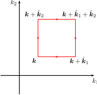
Figure 2: Path along a plaquette for the Fukui-Hatsugai-Suzuki’s method.

II.2 Coh-Vanderbilt’s method

On the other hand, Coh and Vanderbilt related the Chern number and the electronic polarization by flux insertion [33]. Later, this method has been discussed in details by Kang, Lee, and Cho [35]. In this method, the Chern number is given by the following relations,

$$z(\phi) =\braket{\Psi_{0}(0,\phi)}{U_{1}}{\Psi_{0}(0,\phi)}$$ (6a)

$$=-\prod_{\bm{k}}V_{\bm{k}+\frac{\phi}{2\pi}\hat{\bm{k}}_{2},\bm{k}+\frac{\phi}{2\pi}\hat{\bm{k}}_{2}-\hat{\bm{k}}_{1}},$$ (6b)

$$\nu =-\frac{\partial}{\partial\phi}\mathrm{Im\,ln\,}z(\phi)$$ (6c)

where the polarization operator along $\mu$ direction is

$$U_{\mu}=\exp\left(\,{\rm i}\frac{2\pi}{L_{\mu}}\sum_{\bm{r}}x_{\mu}\,n_{\bm{r}}\right).$$ (7)

This is the twist operator introduced in the LSM theorem for $d\geq 2$ [27, 28]. $\ket{\Psi_{0}(\phi_{1},\phi_{2})}$ is the many-body ground state as a function of the flux $\phi_{\mu}$. The Chern number $\nu$ is quantized in the thermodynamic limit.

As discussed in Appendix A, the Chern number in the continuum limit is given by different gauges as that of FHS’s method. Wheres the gauge of FHS’s method is like the symmetric gauge, that of CV’s method corresponds to the Landau gauge. However, we can modify the CV’s method so that the Chern number is given by symmetric gauge. For example, we define the polarization as follows,

$$z(\phi) =\braket{\Psi_{0}(\phi,\phi)}{U_{1}^{\mathstrut}U_{2}^{-1}}{\Psi_{0}(\phi,\phi)}$$ (8)

$$=-\prod_{\bm{k}}V_{\bm{k}+\frac{\phi}{2\pi}(\hat{\bm{k}}_{1}+\hat{\bm{k}}_{2}),\bm{k}+\frac{\phi}{2\pi}(\hat{\bm{k}}_{1}+\hat{\bm{k}}_{2})-\hat{\bm{k}}_{1}+\hat{\bm{k}}_{2}}.$$ (9)

This gives the same representation for $L_{1}=L_{2}$ as that of FHS’s method in the continuum limit.

III Spiral Boundary Conditions

For 2D systems, the exponential position operator with SBCs is given by

$$U_{\rm SBC}=\exp\left({\rm i}\sum_{j=1}^{L}\frac{2\pi jn_{j}}{L}\right),\qquad L=L_{1}L_{2},$$ (10)

where $j$ is the site number of the extended 1D chain which sweeps all lattice sites in 1D order as shown in Fig.1(b). On the other hand, for conventional PBCs as in Fig.1(a), there are two operators as Eq. (7). In this section, we discuss the relationship between $U_{\rm SBC}$ and $U_{\mu}$ for 2D, and how the wave number $\bm{k}$ appearing in Sec. II should be replaced for SBCs.

III.1 Definition of spiral boundary conditions

In order to consider the flux insertion to the system with SBCs, we reinterpret the twist operators in the Oshikawa’s argument (7). First, we consider the unit vectors in the real space and the inverse lattice space of 2D systems as

$$\bm{A}_{1} =(L_{1},0), \qquad\bm{B}_{1} =2\pi(\tfrac{1}{L_{1}},0),$$ (11a)

$$\bm{A}_{2} =(0,L_{2}), \bm{B}_{2} =2\pi(0,\tfrac{1}{L_{2}}).$$ (11b)

Then these vectors satisfy the following relation,

$$\bm{A}_{\mu}\cdot\bm{B}_{\nu}=2\pi\delta_{\mu,\nu}.$$ (12)

The twist operator (7) is written using the above unit vectors in the inverse lattice space as

$$U_{\mu}=\exp\left({\rm i}\sum_{\bm{r}}\bm{B}_{\mu}\cdot\bm{r}n_{\bm{r}}\right).$$ (13)

Next, we choose the unit vectors for SBCs as shown in Fig. 1(b) so that they satisfy the relation (12). Then we have

$$\bm{A}^{\prime}_{1} =(L_{1},-1), \qquad\bm{B}^{\prime}_{1} =2\pi(\tfrac{1}{L_{1}},0),$$ (14a)

$$\bm{A}^{\prime}_{2} =(0,L_{2}), \bm{B}^{\prime}_{2} =2\pi(\tfrac{1}{L_{1}L_{2}},\tfrac{1}{L_{2}}).$$ (14b)

The twist operators in 2D systems with SBCs are introduced as

$$U^{\prime}_{\mu}=\exp\left({\rm i}\sum_{\bm{r}}\bm{B}^{\prime}_{\mu}\cdot\bm{r}n_{\bm{r}}\right).$$ (15)

For $\mu=1$, due to the relation $\bm{B}_{1}^{\prime}=\bm{B}_{1}$, $U_{1}^{\prime}$ is the same operator as $U_{1}$ with SBCs. In order to represent $U_{1}$ in SBCs, we use the following relation

$$\frac{2\pi jn_{j}}{L_{1}}=\frac{2\pi x_{1}n_{\bm{r}}}{L_{1}}\quad(\mathrm{mod}\,2\pi).$$ (16)

For $\mu=2$, the exponent part of the twist operator is confirmed as that of SBCs as

$$\sum_{\bm{r}}\bm{B}^{\prime}_{2}\cdot\bm{r}n_{\bm{r}} =\sum_{i_{1}=1}^{L_{1}}\sum_{i_{2}=0}^{L_{2}-1}2\pi\frac{i_{1}+i_{2}L_{1}}{L_{1}L_{2}}n_{(i_{1},i_{2})}$$ (17)

$$=\sum_{j=1}^{L}\frac{2\pi}{L}jn_{j},$$ (18)

where $L=L_{1}L_{2}$ and $j=i_{1}+i_{2}L_{1}$. Thus the twist operators for SBCs are identified as

$$U_{1}^{\prime} =\exp\left({\rm i}\sum_{j=1}^{L}\frac{2\pi jn_{j}}{L_{1}}\right)=(U_{\rm SBC})^{L_{2}},$$ (19a)

$$U_{2}^{\prime} =U_{\rm SBC}.$$ (19b)

These correspondences mean that the flux insertion for the extended 1D chain of SBCs gives rise an effective current along $y$-direction, while $U_{1}^{\prime}$ causes a current only to $x$-direction due to the relation (16).

In the same way, the unit vectors of the system with SBCs for $(\pi,\pi)$ order illustrated in Fig. 1(c), are identified as

$$\bm{A}^{\prime\prime}_{1} =(L_{1}-1,-1), \bm{B}^{\prime\prime}_{1} =\tfrac{2\pi}{L_{1}L_{2}+L_{1}-L_{2}}(L_{2},-L_{1}),$$ (20a)

$$\bm{A}^{\prime\prime}_{2} =(L_{1},L_{2}), \bm{B}^{\prime\prime}_{2} =\tfrac{2\pi}{L_{1}L_{2}+L_{1}-L_{2}}(1,L_{1}-1).$$ (20b)

Then, the exponential position operators in these SBCs $U_{j}^{\prime\prime}$ for the isotropic case $L_{1}=L_{2}$ are related as

$$U_{1}^{\prime\prime}=U_{1}^{\mathstrut}U_{2}^{-1},\qquad U_{2}^{\prime\prime}=U_{\rm SBC}.$$ (21)

Since we are not interested in charge orders in this paper, we will not use these boundary conditions.

III.2 Redefinition of Coh-Vanderbilt’s method

In the Coh-Vanderbilt method, we need to apply flux to the system to generate a current in the vertical direction of the twist operator for calculating the Chern number. However, since the flux is continuum number, we can not distinguish whether the direction of the flux is along $\bm{B}_{1}^{\prime}$ or $\bm{B}_{2}^{\prime}$. On the other hand, roles of twist operators for each directions are apparently distinguished as in Eq. (19). Therefore, we apply the flux to $\bm{B}_{2}^{\prime}$ direction which is along the extended 1D chain, and turn our attention to the response to $\bm{B}_{1}^{\prime}$ direction.

It follows from Eq. (19) that the expectation value of the twist operator with flux (6a) for the system with SBCs is redefined as

$$z^{\prime}(\phi)=\braket{\Psi_{0}^{\prime}(\phi)}{U_{1}^{\prime}}{\Psi_{0}^{\prime}(\phi)},$$ (22)

where $\ket{\Psi_{0}^{\prime}(\phi)}$ is the many-body wave function of the ground state with flux $\phi$. The flux $\phi$ is imposed to the extended 1D chain with $L=L_{1}L_{2}$ sites. From Eq. (6), the following relation is satisfied,

$$z^{\prime}(\phi)={\rm e}^{-{\rm i}\nu\phi}z^{\prime}(0).$$ (23)

If we consider the expectation value of $U_{2}^{\prime}$ as

$$z_{2}^{\prime}(\phi)=\braket{\Psi_{0}^{\prime}(\phi)}{U_{2}^{\prime}}{\Psi_{0}^{\prime}(\phi)},$$ (24)

we can not detect the Chern number, because the applied current by the flux and its response are in the parallel directions and there is no perpendicular component in the response.

III.3 Correspondence of wave numbers

Now we discuss the correspondence of the wave numbers defined in 2D PBCs with those of SBCs. Let us consider a tight-biding model defined on a 2D square lattice. When we apply SBCs to this system, the hopping term is written as

$$\mathcal{H}= -t\sum_{i=1}^{L}\left[(c_{i}^{{\dagger}}c_{i+1}^{\mathstrut}+\mbox{H.c.})+(c_{i}^{{\dagger}}c_{i+\Lambda}^{\mathstrut}+\mbox{H.c.})\right]$$

$$= -2t\sum_{k}\left[\cos k+\cos\Lambda k\right]c_{k}^{{\dagger}}c_{k}^{\mathstrut},$$ (25)

where $i$ is the number of the lattice sites of the extended 1D chain with $L\equiv L_{1}L_{2}$ sites, and $\Lambda$ is a parameter depending on the number of lattice sites in $x$-direction. As shown in Fig. 1, this parameter is related to ways to label the sites of extended 1D chain and $\Lambda\in\mathbb{Z}$. For SBCs for $(\pi,0)$ order $\Lambda=L_{1}$ while those for $(\pi,\pi)$ order, $\Lambda=L_{1}-1$ . In the present case, we are not interested in charge orders, so that we choose SBCs for $(\pi,0)$ order for simplicity. The Fourier transformation of the extended 1D chain is given by

$$c_{k,\alpha}=\frac{1}{\sqrt{L}}\sum_{j=1}^{L}{\rm e}^{-{\rm i}kx_{j}}c_{j,\alpha}.$$ (26)

Then the 2D wave vectors are replaced as the 1D wave number by

$$\bm{k}=(k_{x},k_{y})\to(k,L_{1}k),$$ (27a)

$$k=\frac{2\pi}{L}n,\qquad n=0,1,2,\cdots,L,$$ (27b)

Next we consider the unit wave numbers $\hat{\bm{k}}_{\mu}$ ($\mu=1,2$) appearing in Sec. II. According to the results of $\bm{B}_{\mu}^{\prime}$ given in Eq. (14), there are following relations,

$$\hat{\bm{k}}_{1} =(\hat{k}_{1},0)\to(L_{2}\hat{k},0),$$ (28a)

$$\hat{\bm{k}}_{2} =(0,\hat{k}_{2})\to(\hat{k},L_{1}\hat{k}),$$ (28b)

where

$$\hat{k}_{\mu}=\frac{2\pi}{L_{\mu}},\qquad\hat{k}=\frac{2\pi}{L}.$$ (29)

Then $Z(\bm{k})$ defined by Eq. (3a) and $z$ by Eq. (6b) are replaced as

$$Z(\bm{k})\to V_{(k,L_{1}k),(k+L_{2}\hat{k},L_{1}k)}V_{(k+L_{2}\hat{k},L_{1}k),(k+L_{2}\hat{k}+\hat{k},L_{1}k+L_{1}\hat{k})}$$

$$\times V_{(k+L_{2}\hat{k}+\hat{k},L_{1}k+L_{1}\hat{k}),(k+\hat{k},L_{1}k+L_{1}\hat{k})}V_{(k+\hat{k},L_{1}k+L_{1}\hat{k}),(k,L_{1}k)},$$ (30)

$$z^{\prime}(\phi)\to-\prod_{k}V_{(k+\tfrac{\phi}{L},L_{1}k+\tfrac{\phi}{L_{2}}),(k+\tfrac{\phi}{L}-L_{2}\hat{k},L_{1}k+\tfrac{\phi}{L_{2}})}.$$ (31)

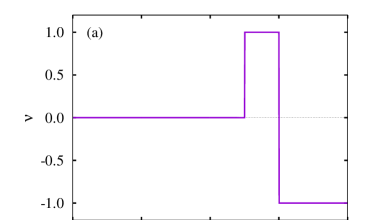
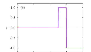
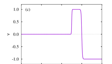
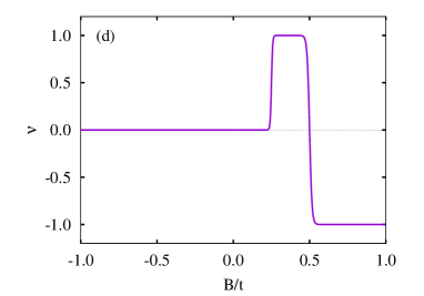
Figure 3: Chern numbers of the 2D WD model with $M/t=1$ and $L=64\times 64$ sites calculated by Fukui-Hatsugai-Suzuki’s method for (a) conventional PBCs and (b) SBCs, and those calculated by Coh-Vanderbilt’s method for (c) conventional PBCs and (d) SBCs. Topological regions are $1/4\leq B/t\leq 1/2$ with $\nu=1$ and $1/2\leq B/t$ with $\nu=-1$.

IV Results

We demonstrate the above discussions in representative models for Chern insulators: the Wilson-Dirac model and the Haldane model.

IV.1 Wilson-Dirac model

As a fundamental model to describe 2D Chern insulators, we consider the Wilson-Dirac model [31, 32],

$$\mathcal{H}= \frac{-{\rm i}t}{2}\sum_{j,\mu=x,y}(c_{j}^{{\dagger}}\tau_{\mu}c_{j+\hat{\mu}}^{\mathstrut}-\mathrm{H.c.})+(M-B)\sum_{j}c_{j}^{{\dagger}}\tau_{3}c_{j}^{\mathstrut}$$

$$+\frac{B}{2}\sum_{j,\mu=x,y}(c_{j}^{{\dagger}}\tau_{3}c_{j+\hat{\mu}}^{\mathstrut}+\mathrm{H.c.}).$$ (32)

The Fourier representation of this model becomes

$$\mathcal{H}= \sum_{\bm{k},\alpha,\beta}c^{\dagger}_{\bm{k},\alpha}\,H_{\alpha\beta}(\bm{k})\,c^{\mathstrut}_{\bm{k},\beta},$$ (33a)

$$H(\bm{k})= t\sum_{\mu=x,y}\sin k_{\mu}\,\tau_{\mu}+\left[M-B\sum_{\mu=x,y}\bigl{(}1-\cos k_{\mu}\bigr{)}\right]\tau_{z},$$ (33b)

where $t$ is the hopping amplitude, $M$ is the mass, $B$ is the coefficient of the Wilson term, $c_{\bm{k},\alpha}$ is the annihilation operator of a fermion with a 2D wave number, $\alpha,\beta$ are orbital indices, and $\tau_{\mu}$ are the Pauli matrices. The energy eigenvalue is given by

$$\varepsilon_{\bm{k}}^{2}=t^{2}(\sin^{2}k_{x}+\sin^{2}k_{y})+\bigl{\{}M-B(2-\cos k_{x}-\cos k_{y})\bigr{\}}^{2}.$$ (34)

This system is a trivial insulator for $B/t<M/4t$, and a topological insulator with $\nu=1$ for $M/4t\leq B/t\leq M/2t$ and that with $\nu=-1$ for $M/2t\leq B/t$. Topological phase transition occurs at $B=M/4$ and $M/2$ [36]. These transition points can be identified by vanishing of the bulk energy gap $\varepsilon_{\bm{k}}=0$. In the continuum version of the model, the Hall conductivity is calculated as [37]

$$\sigma_{xy}=-\frac{e^{2}}{2h}[{\rm sgn}(M)+{\rm sgn}(B)].$$ (35)

Therefore the system is a topological (trivial) insulator for $MB>0$ ($MB<0$), and a topological transition occurs at $B=0$ for fixed $M$.

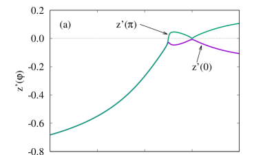
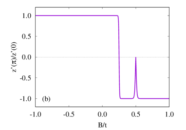
Figure 4: (a) Expectation values of the twist operator $U_{1}^{\prime}$ with and without flux, $z^{\prime}(0)$ and $z^{\prime}(\pi)$. (b) The ratio of the expectation values $z^{\prime}(\pi)/z^{\prime}(0)$. There is no sign change for $z^{\prime}(0)$, while $z^{\prime}(\pi)$ has the opposite sign in the topological regions. These results are calculated for the systems with $M/t=1$ and $L=64\times 64$ sites.

As shown in Fig. 3, the Chern number of the WD model obtained by the FHS method and the CV method with conventional PBCs and SBCs. The finite-size effect of the FHS method tends to be smaller than that of the CV method, and that of the conventional PBCs tends to be smaller than the SBCs.

Figure 4(a) shows $z^{\prime}(\phi)$, the ground-state expectation values of the twist operator $U_{1}^{\prime}$ in SBCs. According to the results, $z^{\prime}(0)$ does not change the sign. On the other hand, $z^{\prime}(\pi)$ changes the sign in the topological regions $M/4<B$ with the Chern number $\nu=\pm 1$, due to the relation (23). We can also identify the topological regions by calculating the ratio of the expectation values of $U_{1}^{\prime}$ with and without flux $z^{\prime}(\pi)/z^{\prime}(0)$ as shown in Fig. 4(b).

In case we consider the expectation value of $U_{\rm SBC}$ as (24), it has the opposite sign in the second topological region $M/2<B$, and that with different SBCs shown in Fig. 1(c) has opposite sign in the both two topological regions $M/4<B$. These results are already discussed in Ref. 26.

IV.2 Haldane model

As another fundamental model for a Chern insulator, we consider the Haldane model [1] describing the fermions on a honeycomb lattice with an alternating potential $M$ and a next-nearest neighbor hopping $\kappa$,

$$\mathcal{H}=t\sum_{\braket{ij}}c_{i}^{\dagger}c_{j}^{\mathstrut}+M\sum_{i}\eta_{i}c_{i}^{\dagger}c_{i}^{\mathstrut}+{\rm i}\frac{\kappa}{3\sqrt{3}}\sum_{\braket{\braket{ij}}}\nu_{ij}c_{i}^{\dagger}c_{j}^{\mathstrut},$$ (36)

where $c_{i}^{{\dagger}}$ ($c_{i}$) is a creation (annihilation) operator at site $i$ (spin indices are omitted). $\braket{ij}$ and $\braket{\braket{ij}}$, denote a nearest and a next nearest pair, respectively. $\eta_{i}=1$ ($\eta_{i}=-1$) for A (B) sublattice, and $\nu_{ij}=(2/\sqrt{3})(\hat{\bm{d}}_{1}\times\hat{\bm{d}}_{2})_{z}=\pm 1$, where $\hat{\bm{d}}_{1}$ and $\hat{\bm{d}}_{2}$ are unit vectors along the two bonds on which the electron hops from a site $j$ to $i$, as shown in Fig. 5.

For the honeycomb lattice, the fundamental vectors are

$$\bm{a}_{1}=\frac{a}{2}(3,\sqrt{3}),\qquad\bm{a}_{2}=\frac{a}{2}(3,-\sqrt{3}).$$ (37)

Then the reciprocal lattice vectors are chosen as

$$\bm{b}_{1}=\frac{2\pi}{3a}(1,\sqrt{3}),\qquad\bm{b}_{2}=\frac{2\pi}{3a}(1,-\sqrt{3}),$$ (38)

by the following relation,

$$\bm{a}_{i}\cdot\bm{b}_{j}=2\pi\delta_{ij}.$$ (39)

The wave numbers are given in these bases as

$$\bm{k}=k_{1}\bm{b}_{1}+k_{2}\bm{b}_{2},$$ (40)

where $k_{i}\in[-\pi,\pi]$.

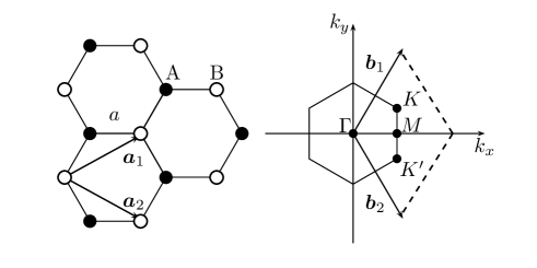
Figure 5: Unit vectors and reciprocal lattice vectors of the honeycomb lattice.

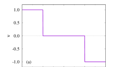
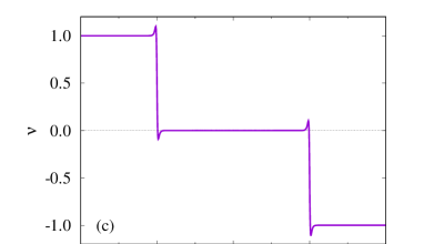
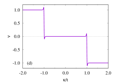
Figure 6: Chern numbers of the Haldane model with $M/t=1$ and $L=64\times 64$ sites calculated by Fukui-Hatsugai-Suzuki’s method for (a) conventional PBCs and (b) SBCs, and those calculated by Coh-Vanderbilt’s method for (c) conventional PBCs and (d) SBCs. Topological regions are $\kappa/t\leq-1$ with $\nu=1$ and $1\leq\kappa/t$ with $\nu=-1$.

The Hamiltonian in the momentum space has the following form,

$$H(\bm{k})=d_{i}(\bm{k})\tau_{i},$$ (41)

with the energy

$$\varepsilon(\bm{k})=\pm\sqrt{\sum_{i}d^{2}_{i}(\bm{k})}.$$ (42)

The parameters in Hamiltonian are given as follows,

$$d_{1} =t[\cos(\bm{k}\cdot\bm{a}_{1})+\cos(\bm{k}\cdot\bm{a}_{2})+1],$$ (43a)

$$d_{2} =t[\sin(\bm{k}\cdot\bm{a}_{1})+\sin(\bm{k}\cdot\bm{a}_{2})],$$ (43b)

$$d_{3} =M+\frac{2\kappa}{3\sqrt{3}}$$

$$\times [\sin(\bm{k}\cdot\bm{a}_{1})-\sin(\bm{k}\cdot\bm{a}_{2})-\sin(\bm{k}\cdot(\bm{a}_{1}-\bm{a}_{2}))].$$ (43c)

Thus we can calculate the Chern number as in the same way of the square lattice systems, by using the wave vector as $\bm{k}=(k_{1},k_{2})$.

Then the Hall conductivity of the system at the charge neutrality point becomes

$$\sigma_{xy}=\frac{e^{2}}{h}{\rm sgn}(\kappa)\theta(|\kappa|-|M|).$$ (44)

This means that the system is a Chern insulator for $|\kappa|>|M|$ with $\nu=\pm 1$ and a trivial insulator for $|\kappa|<|M|$ with $\nu=0$.

Figure 6 shows the Chern number of the Haldane model is obtained by the FHS method and the CV method with conventional PBCs and SBCs. Finite-size effect of the FHS method tends to be smaller than that of the CV method, and that of the conventional PBCs tends to be smaller than the SBCs. These tendencies are same for the WD model.

Figure 7(a) shows the ground-state expectation values of the twist operators in SBCs $z^{\prime}(\phi)$ without flux. The result of $z^{\prime}(0)$ has large finite-size effects with oscillations, so that it is difficult to characterize the insulating states and electronic polarization. This behavior is considered to be an effect of the next nearest neighbor hopping process. However, the ratio of $z^{\prime}(\phi)$ with and without flux $z^{\prime}(\pi)/z^{\prime}(0)$, this well characterizes the topological regions $|\kappa|<|M|$ as shown in Fig. 7(b).

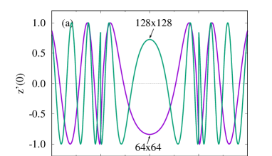
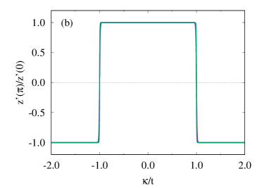
Figure 7: (a) Expectation values of twist operators $U_{1}^{\prime}$ without flux $z^{\prime}(0)$. (b) The ratio of the expectation values of $U_{1}^{\prime}$ with and without flux $z^{\prime}(\pi)/z^{\prime}(0)$ calculated in the systems with $L=64\times 64$ and $L=128\times 128$.

V Summary and discussion

In summary, we have explored the relationship between electronic polarization and the Chern number in 2D systems with SBCs. Initially, we examined two methods for calculating Chern numbers in 2D lattice systems: Fukui-Hatsugai-Suzuki’s method and Coh-Vanderbilt’s method. Subsequently, we introduced twist operators in 2D systems with SBCs and redefined the aforementioned methods using the wave numbers of the extended 1D chain. The crucial aspect of this discussion is that flux insertion into the extended 1D chain generates an effective current along the $y$-direction, and the twist operator detects the response to the $x$-direction. Finally, we illustrated the above discussions in representative models for Chern insulators, such as the Wilson-Dirac model and the Haldane model, demonstrating that the calculation of Chern numbers and the detection of topological phases are achievable using methods with SBCs.

The relationship between topological states in 1D and those in 2D with a Chern number is considered as follows: As mentioned in Sec. I, the signs of $z$ classify 1D gapped states, and in some cases, such as the Su-Schrieffer-Heeger model [38, 39], an insulating state with localized edge electrons emerges. If we then consider creating a 2D system by connecting these 1D edge states with spiral boundary conditions (SBCs), an insulating state with edge current may appear in response to applied flux. This state represents a 2D topological state with a Chern number.

As an extension of the argument presented in this paper, we may consider SBCs in general dimensions. According to the discussion in Sec. III, the twist operators in $d$-dimensional systems are generalized as follows:

$$U^{\prime}_{\mu}=\exp\left({\rm i}\sum_{j=1}^{L}\frac{2\pi jn_{j}}{\prod_{k=1}^{\mu}L_{k}}\right),\quad L=\prod_{k=1}^{d}L_{k}.$$ (45)

By utilizing these operators and incorporating flux insertions, we may identify $d$-dimensional topological phases and higher-order topological states.

The present method with SBCs is expected to be applicable to numerical calculations, such as the density matrix renormalization group method. For systems in more than 2D, finite-size scaling is not as straightforward as in 1D systems because increasing the number of lattice sites cannot be done linearly while maintaining the symmetry of the unit systems. However, in systems with SBCs, we can increase the lattice size linearly, enabling finite-size scaling similar to 1D systems [40, 41, 42]. We anticipate that the present method will prove useful for the numerical analysis of topological systems with electron-electron interactions.

VI Acknowledgments

M. N. acknowledges the research fellow position of the Institute of Industrial Science, The University of Tokyo. M. N. is supported partly by MEXT/JSPS KAKENHI Grant Number JP20K03769. The authors thank S. Nishimoto and H. Watanabe for helpful discussions.

Appendix A Continuum limit

In this section, we discuss the continuum limits of the formulas for the Chern number given by the Fukui-Hatsugai-Suzuki’s method and by the Coh-Vanderbilt’s method for lattice systems, to compare the Thouless-Kohmoto-Nightingale-den Nijs (TKNN) formula.

A.1 TKNN formula

Let’s consider a 2D system. When the system is translationally invariant, the Hamiltonian satisfies the following eigenvalue equation in term of the Bloch state,

$$H(\bm{k})\ket{u_{n}(\bm{k})}=E_{n}(\bm{k})\ket{u_{n}(\bm{k})},$$ (46)

where $\ket{u_{n}(\bm{k})}$ is the Bloch eigenstate of the $n$-th band, and normalized as $\braket{u_{n}(\bm{k})}{u_{m}(\bm{k})}=\delta_{n,m}$. The Berry connection of the $n$-th band is defined as

$$\bm{A}^{(n)}(\bm{k})={\rm i}\braket{u_{n}(\bm{k})}{\nabla_{\bm{k}}u_{n}(\bm{k})}.$$ (47)

Then the Berry curvature is given as

$$\bm{B}^{(n)}(\bm{k})=\nabla_{\bm{k}}\times\bm{A}^{(n)}(\bm{k}).$$ (48)

The Berry connection and the Berry curvature correspond to the vector potential and the magnetic field in the electrodynamics, respectively.

The Chern number for the $n$-th band $\nu_{n}$ is given by the Berry curvature as follows,

$$\nu_{n} =\frac{1}{2\pi}\iint_{\rm BZ}{\rm d}^{2}\bm{k}\,[\bm{B}^{(n)}(\bm{k})]_{z}$$

$$=\frac{1}{2\pi}\oint_{\partial{\rm BZ}}{\rm d}\bm{k}\cdot\bm{A}^{(n)}(\bm{k}),$$ (49)

where BZ means the 1st Brillouin zone. Then the Chern number $\nu$ is given by the summation of $\nu_{n}$ over the occupied bands, and the Hall conductivity is related to the Chern number as follows,

$$\sigma_{xy}=-\nu\frac{e^{2}}{h},\qquad\nu=\sum_{n\in{\rm occupied}}\nu_{n}.$$ (50)

This is so-called TKNN formula [43, 44, 45, 46].

A.2 Fukui-Hatsugai-Suzuki’s method

Now we show that the Chern numbers in lattice systems are related to those defined in the continuous Brillouin zone (49) in the continuum limit. By the Taylor expansion, $V_{\bm{k},\bm{k}+\hat{k}_{\mu}}$ defined by Eq. (2) in the continuum limit becomes

$$V_{\bm{k},\bm{k}+\hat{k}_{\mu}}\simeq 1-{\rm i}\frac{2\pi}{L_{\mu}}A_{\mu}(\bm{k}),$$ (51)

where $A_{\mu}(\bm{k})$ is the Berry connection defined in (47). Similarly, we get

$$V_{\bm{k}+\hat{k}_{\mu},\bm{k}+\hat{k}_{\mu}+\hat{k}_{\nu}} \simeq 1-{\rm i}\frac{2\pi}{L_{\nu}}A_{\nu}(\bm{k}+\hat{k}_{\mu})$$ (52)

$$\simeq 1-{\rm i}\frac{2\pi}{L_{\nu}}A_{\nu}(\bm{k})-{\rm i}\frac{(2\pi)^{2}}{L_{\mu}L_{\nu}}\partial_{\mu}A_{\nu}(\bm{k}),$$

where $\mu\neq\nu$, and we have abbreviated as $\partial_{\nu}=\partial_{k_{\nu}}$. Next, $F_{12}(\bm{k})$ defined by Eq. (3) becomes

$$F_{12}(\bm{k}) \simeq\ln\Biggl{[}\left(1-{\rm i}\frac{2\pi}{L_{1}}A_{1}\right)\left(1-{\rm i}\frac{2\pi}{L_{2}}A_{2}-{\rm i}\frac{(2\pi)^{2}}{L_{1}L_{2}}\partial_{1}A_{2}\right)\left(1+{\rm i}\frac{2\pi}{L_{1}}A_{1}+{\rm i}\frac{(2\pi)^{2}}{L_{1}L_{2}}\partial_{2}A_{1}\right)\left(1+{\rm i}\frac{2\pi}{L_{2}}A_{2}\right)\Biggr{]}$$

$$\simeq\ln\left[1-{\rm i}\frac{(2\pi)^{2}}{L_{1}L_{2}}\bigl{(}\partial_{1}A_{2}-\partial_{2}A_{1}\bigr{)}\right]$$

$$\simeq-{\rm i}\frac{(2\pi)^{2}}{L_{1}L_{2}}\bigl{(}\partial_{1}A_{2}-\partial_{2}A_{1}\bigr{)},$$ (53)

so that the Chern number in lattice systems (5) becomes

$$\nu\simeq\frac{1}{2\pi}\iint{\rm d}^{2}\bm{k}\bigl{[}\partial_{1}A_{2}(\bm{k})-\partial_{2}A_{1}(\bm{k})\bigr{]}.$$ (54)

This coincides with the TKNN formula (49).

A.3 Coh-Vanderbilt’s method

The relations of the Coh-Vanderbilt’s (CV’s) method (6) are confirmed by the following calculations,

$$\prod_{\bm{k}}\braket{u(k_{1},k_{2}+\tfrac{\phi}{L_{2}})}{u(k_{1}-\tfrac{2\pi}{L_{1}},k_{2}+\tfrac{\phi}{L_{2}})} \simeq\prod_{\bm{k}}\left(1-\frac{2\pi}{L_{1}}\braket{u(k_{1},k_{2}+\tfrac{\phi}{L_{2}})}{\partial_{1}u(k_{1},k_{2}+\tfrac{\phi}{L_{2}})}\right)$$

$$\simeq\exp\biggl{[}\,{\rm i}\frac{L_{2}}{2\pi}\iint{\rm d}^{2}\bm{k}\,A_{1}(k_{1},k_{2}+\tfrac{\phi}{L_{2}})\biggr{]}$$

$$\simeq\exp\biggl{[}\,{\rm i}\frac{L_{2}}{2\pi}\iint{\rm d}^{2}\bm{k}\,A_{1}(k_{1},k_{2})\biggr{]}\exp\biggl{[}\,{\rm i}\phi\underbrace{\frac{1}{2\pi}\iint{\rm d}^{2}\bm{k}\,\partial_{2}A_{1}(k_{1},k_{2})}_{-\nu}\biggr{]}.$$ (55)

In this case, the Chern number is given by the Landau gauge, wheres the FHS’s method is corresponds to the symmetric gauge. Thus we get the relation

$$z(0,\phi)=z(0,0){\rm e}^{-{\rm i}\phi\,\nu}.$$ (56)

Similarly, we get

$$\braket{\Psi_{0}(\phi,0)}{U_{2}}{\Psi_{0}(\phi,0)}\sim z(0,0){\rm e}^{{\rm i}\phi\,\nu}.$$ (57)

Thus we have shown that the relationship between $z(\phi)$ and the Chern number $\nu$ are given by Eq (6c).

However, we can modify the CV’s method so that the Chern number is given by the symmetric gauge. For this purpose, we define the polarization as follows,

$$z(\phi) =\braket{\Psi_{0}(\phi,\phi)}{U_{1}^{\mathstrut}U_{2}^{-1}}{\Psi_{0}(\phi,\phi)}$$

$$=-\prod_{\bm{k}}\braket{u(k_{1}+\tfrac{\phi}{L_{1}},k_{2}+\tfrac{\phi}{L_{2}})}{u(k_{1}+\tfrac{\phi}{L_{1}}-\tfrac{2\pi}{L_{1}},k_{2}+\tfrac{\phi}{L_{2}}+\tfrac{2\pi}{L_{2}})}.$$ (58)

Then (58) becomes

$$z(\phi_{1},\phi_{2})=-\prod_{\bm{k}}\braket{u(k_{1}+\tfrac{\phi_{1}}{L_{1}},k_{2}+\tfrac{\phi_{2}}{L_{2}})}{u(k_{1}+\tfrac{\phi_{1}-2\pi}{L_{1}},k_{2}+\tfrac{\phi_{2}+2\pi}{L_{2}})}.$$ (59)

In the thermodynamic limit $L_{\mu}\gg 1$, the Taylor expansion gives

$$z(0,0) =-\prod_{\bm{k}}\braket{u(k_{1},k_{2})}{u(k_{1}-\tfrac{2\pi}{L_{1}},k_{2}+\tfrac{2\pi}{L_{2}})}$$

$$\simeq-\exp\left[{\rm i}\iint{\rm d}^{2}\bm{k}\left\{\frac{L_{2}}{2\pi}A_{1}(k_{1},k_{2})-\frac{L_{1}}{2\pi}A_{2}(k_{1},k_{2})\right\}\right],$$ (60)

where $A_{\mu}(k_{1},k_{2})$ is a component of the Berry connection defined in Eq. (47). Therefore Eq. (58) becomes

$$z(\phi_{1},\phi_{2}) =-\exp\left[{\rm i}\iint{\rm d}^{2}\bm{k}\left\{\frac{L_{2}}{2\pi}A_{1}(k_{1}+\tfrac{\phi_{1}}{L_{1}},k_{2}+\tfrac{\phi_{2}}{L_{2}})-\frac{L_{1}}{2\pi}A_{2}(k_{1}+\tfrac{\phi_{1}}{L_{1}},k_{2}+\tfrac{\phi_{2}}{L_{2}})\right\}\right]$$

$$=z(0,0)\exp\left[{\rm i}\iint{\rm d}^{2}\bm{k}\left\{\frac{L_{2}}{L_{1}}\frac{\phi_{1}}{2\pi}\partial_{1}A_{1}(\bm{k})+\frac{\phi_{2}}{2\pi}\partial_{2}A_{1}(\bm{k})-\frac{\phi_{1}}{2\pi}\partial_{1}A_{2}(\bm{k})-\frac{L_{1}}{L_{2}}\frac{\phi_{2}}{2\pi}\partial_{2}A_{2}(\bm{k})\right\}\right]$$

$$\simeq z(0,0)\exp\left[-{\rm i}\frac{\phi}{2\pi}\iint{\rm d}^{2}\bm{k}(\partial_{1}A_{2}(\bm{k})-\partial_{2}A_{1}(\bm{k}))\right],\qquad(\phi=\phi_{1}=\phi_{2},\,L_{1}=L_{2})$$

$$=z(0,0)\exp(-{\rm i}\phi\,\nu).$$ (61)

Thus we have obtained the Chern number given by the symmetric gauge.

References

- [1] F. D. M. Haldane, Phys. Rev. Lett. 61, 2015 (1988).
- [2] C. L. Kane and E. J. Mele, Phys. Rev. Lett. 95, 146802 (2005).
- [3] B. A. Bernevig and S. C. Zhang, Phys. Rev. Lett. 96, 106802 (2006).
- [4] B. A. Bernevig, T. L. Hughes, and S. C. Zhang, Science 314, 1757 (2006).
- [5] S. Ryu, A. P. Schnyder, A. Furusaki, and A.W. Ludwig, New J. Phys. 12, 065010 (2010).
- [6] M. König, S. Wiedmann, C. Brüne, A. Roth, H. Buhmann, L. W. Molenkamp, X.-L. Qi, and S.-C. Zhang, Science, 318, 766 (2007).
- [7] M. König, H. Buhmann, L. W. Molenkamp, T. Hughes, C.-X. Liu, X.-L. Qi, and S.-C. Zhang, J. Phys. Soc. Jpn. 77, 031007 (2008).
- [8] N. Read and D. Green, Phys. Rev. B 61, 10267 (2000).
- [9] A. Y. Kitaev, Ann. Phys. (N.Y.), 321, 2 (2006).
- [10] S. Yao and Z. Wang, Phys. Rev. Lett. 121, 086803 (2018).
- [11] F. D. M. Haldane, Phys. Rev. B 25, 4925(R) (1982).
- [12] F. D. M. Haldane, Phys. Lett. A93, 464 (1983).
- [13] F. D. M. Haldane, Phys. Rev. Lett. 50, 1153 (1983).
- [14] I. Affleck and F. D. M. Haldane, Phys. Rev. B 36, 5291 (1987).
- [15] R. Resta, Rev. Mod. Phys. 66, 899 (1994).
- [16] R. Resta, Phys. Rev. Lett. 80, 1800 (1998).
- [17] R. Resta and S. Sorella, Phys. Rev. Lett. 82, 370 (1999).
- [18] R. Resta, J. Phys. Condens. Matter 12, R107 (2000).
- [19] M. Nakamura and J. Voit, Phys. Rev. B 65, 153110 (2002).
- [20] M. Nakamura and S. Todo, Phys. Rev. Lett. 89, 077204 (2002).
- [21] E. Lieb, T. Schultz, and D. Mattis, Ann. Phys. (Amsterdam) 16, 407 (1961).
- [22] I. Affleck and E. H. Lieb, Lett. Math. Phys. 12, 57 (1986).
- [23] I. Affleck, Phys. Rev. B 37, 5186 (1988).
- [24] M. Oshikawa, M. Yamanaka, and I. Affleck, Phys. Rev. Lett. 78, 1984 (1997).
- [25] M. Yamanaka, M. Oshikawa, and I. Affleck, Phys. Rev. Lett. 79, 1110 (1997).
- [26] M. Nakamura, S. Masuda, and S. Nishimoto, Phys. Rev. B 104, L121114 (2021).
- [27] M. Oshikawa, Phys. Rev. Lett. 84, 1535 (2000).
- [28] M. Oshikawa, Phys. Rev. Lett. 84, 3370 (2000).
- [29] M. B. Hastings, Europhys. Lett. 70, 824 (2005).
- [30] Y. Yao and M. Oshikawa, Phys. Rev. X 10, 031008 (2020).
- [31] K. G. Wilson, Phys. Rev. D 10, 2445 (1974).
- [32] X. L. Qi, Y. S. Wu, and S. C. Zhang, Phys. Rev. B 74, 085308 (2006).
- [33] S. Coh and D. Vanderbilt, Phys. Rev. Lett. 102, 107603 (2009).
- [34] T. Fukui, Y. Hatsugai, and H. Suzuki, J. Phys. Soc. Jpn. 74, 1674 (2005).
- [35] B. Kang, W. Lee, and G. Y. Cho, Phys. Rev. Lett. 126, 016402 (2021).
- [36] K. Imura, A. Yamakage, S.J. Mao, A. Hotta, Y. Kuramoto, Phys. Rev. B 82, 085118 (2010).
- [37] H. So, Prog. Theor. Phys. 73, 528 (1985).
- [38] W. P. Su, J. R. Schrieffer, and A. J. Heeger, Solitons in Polyacetylene, Phys. Rev. Lett. 42, 1698 (1979).
- [39] W. P. Su, J. R. Schrieffer, and A. J. Heeger, Soliton excitations in polyacetylene, Phys. Rev. B 22, 2099 (1980).
- [40] M. Kadosawa, M. Nakamura, Y. Ohta, and S. Nishimoto, Phys. Rev. B 107, L081104 (2023).
- [41] M. Kadosawa, M. Nakamura, Y. Ohta, and S. Nishimoto, J. Phys. Soc. Jpn. 92, 023701 (2023).
- [42] M. Kadosawa, M. Nakamura, Y. Ohta, and S. Nishimoto, J. Phys. Soc. Jpn. 92, 055001 (2023).
- [43] D. J. Thouless, M. Kohmoto, M. P. Nightingale, and M. den Nijs, Phys. Rev. Lett. 49, 405 (1982).
- [44] J. E. Avron, R. Seiler, and B. Simon, Phys. Rev. Lett. 51, 51 (1983).
- [45] M. Kohmoto, Ann. Phys. 160, 343 (1985).
- [46] Q. Niu, D. J. Thouless, and Y. S. Wu, Phys. Rev. B 31, 3372 (1985).